Control of resistive wall modes in a cylindrical tokamak with plasma rotation and complex gain

Abstract

Feedback stabilization of magnetohydrodynamic (MHD) modes is studied in a cylindrical model for a tokamak with resistivity, viscosity and toroidal rotation. The control is based on a linear combination of the normal and tangential components of the magnetic field just inside the resistive wall. The feedback includes complex gain, for both the normal and for the tangential components, and the imaginary part of the feedback for the former is equivalent to plasma rotation. The work includes (1) analysis with a reduced resistive MHD model for a tokamak with finite $\beta$ and with stepfunction current density and pressure profiles, and (2) computations with full compressible visco-resistive MHD and smooth decreasing profiles of current density and pressure. The equilibria are stable for $\beta=0$ and the marginal stability values $\beta_{rp,rw}<\beta_{rp,iw}<\beta_{ip,rw}<\beta_{ip,iw}$ (resistive plasma, resistive wall; resistive plasma, ideal wall; ideal plasma, resistive wall; ideal plasma, ideal wall) are computed for both cases. The main results are: (a) imaginary gain with normal sensors or plasma rotation stabilizes below $\beta_{rp,iw}$ because rotation supresses the diffusion of flux from the plasma out through the wall and, more surprisingly, (b) rotation or imaginary gain with normal sensors destabilizes above $\beta_{rp,iw}$ because it prevents the feedback flux from entering the plasma through the resistive wall to form a virtual wall. The effect of imaginary gain with tangential sensors is more complicated but essentially destabilizes above and below $\beta_{rp,iw}$. A method of using complex gain to optimize in the presence of rotation in the $\beta>\beta_{rp,iw}$ regime is presented.

${}^{*}$Department of Astrophysical Sciences, Princeton University, Princeton, NJ 08544; ${}^{\dagger}$ Applied Mathematics and Plasma Physics, Theoretical Division, Los Alamos National Laboratory, Los Alamos, NM 87545

1 Introduction

Feedback stabilization of magnetohydrodynamic (MHD) modes with plasma resistivity and a resistive wall in tokamaks has received recent attention particularly because of the need to control disruptions[6, 1, 11, 12, 17, 16, 2, 7, 10, 19, 22, 25]. Studies have also been performed for reversed field pinches (RFPs)[4, 33, 34]. Earlier studies in tokamak geometry[13, 27, 9, 5, 8, 3, 32] investigated sensing either the radial or the poloidal component of the magnetic field, concluding that it is better to sense the poloidal component, and that the latter measurement is of more use inside the wall[32, 13]. Results in Refs. [9, 13] suggested that the advantages of tangential sensing are due to the fact that it is less sensitive to sensors that detect sidebands or feedback coils that excite sidebands.

In Ref. [14] studies were performed with of both the radial and poloidal components (radial and toroidal components in the RFP context) but with idealized (single Fourier component) coils. The results showed that this approach has useful advantages over control based on either sensor alone. Whereas feedback based on sensing either field component alone is limited to the marginal stability point for resistive plasma modes with an ideal wall, feedback based on sensing both components can stabilize up to the ideal plasma - ideal wall limit. These results were presented in Ref. [14], which used a very simple qualitative model based on reduced resistive MHD[35] for the plasma dynamics. More recent investigations in full visco-resistive MHD in a cylindrical model for RFPs[33, 34] have shown this ability to stabilize close to the ideal plasma - ideal wall limit, depending on the plasma viscosity and resistivity. In Ref. [34] the work in Ref. [33] was extended to a model measuring the radial component and two tangential components of the magnetic field, again in RFP geometry. This work included the presence of two walls, the (inner) vacuum vessel and a better conducting external copper shell, with sensors between the two walls, as suggested by the configuration of the RFX-mod facility[28]. The results of this study also showed the possibility of stabilizing close to the ideal plasma - ideal wall limit, depending on the plasma viscosity and the placement of the sensors, and that the second tangential component (toroidal in tokamak geometry and poloidal in RFP geometry) is not important. The RFX-mod facility has the capability of sensing both the normal and toroidal components and applying a pre-specified linear combination of these[31, 29]. In the theoretical work in Refs. [33, 34], the normal and tangential components were considered independent. The RFP results with $\beta=0$ were parameterized in terms of the critical values of the equilibrium current density at the magnetic axis, i.e. $\lambda_{0}=(j_{||}/B)(r=0)$, namely $\lambda_{rp,rw}<\lambda_{rp,iw}<\lambda_{ip,rw}<\lambda_{ip,iw}$. These four values of $\lambda_{0}$ are, respectively the current limits for resistive plasma, resistive wall; resistive plasma, ideal wall; ideal plasma, resistive wall; and ideal plasma, ideal wall. The inner inequality $\lambda_{rp,iw}<\lambda_{ip,rw}$ was observed to hold[33, 34] for all RFP equilibria investigated. The other inequalities must always hold.

In this paper we investigate linear stability in a finite-$\beta$ cylindrical model with tokamak-like profiles, namely large toroidal aspect ratio $R/a$, large toroidal field $B_{z}\sim(R/a)B_{\theta}$ and decreasing profiles of current density $j_{z0}(r)$ and pressure $p_{0}(r)$. The decreasing $j_{z0}(r)$ profile leads to a monotonically increasing profile of the safety factor $q(r)=rB_{z0}/RB_{\theta 0}(r)$ with $q\sim 1$. We consider equilibria which are stable for zero pressure and characterize the stability properties without feedback in terms of the four marginal values of $\beta_{0}=2p_{0}(0)/B_{z0}(0)^{2}$, namely $\beta_{rp,rw}<\beta_{rp,iw}<\beta_{ip,rw}<\beta_{ip,iw}$, analogous to the values of $\lambda=j_{||}/B$ at $r=0$ in the RFP studies. (As in the RFP studies, the middle inequality, which does not hold in general, has been observed to hold for all the equilibria we considered.) We again investigate the behavior with feedback proportional to the radial and poloidal magnetic field components, with gain factors $G$ and $K$, respectively. We also include toroidal plasma rotation and complex gain[26] for both the normal component and the tangential component, i.e. $G$ and $K$. (Complex gain is attained by shifting the phase of the actuator coils relative to the sensor coils.) In Ref. [15] it was argued that, in cylindrical geometry with a single $k_{z}$, the imaginary part $G_{i}=\text{Im}G$ is equivalent to rotation of the wall, which is in turn equivalent to rigid rotation of the plasma.

An aspect of our studies worth emphasizing is the inclusion of plasma resistivity as well as wall resistivity. This inclusion introduces two important marginal stability parameters, namely $\beta_{rp,rw}$ and $\beta_{rp,iw}$, that are absent in ideal MHD. Also, above the latter limit, modes are unstable but grow on the wall time $\tau_{w}$ and are therefore sensitive to plasma resistivity and react differently to plasma rotation.

As in the RFP control studies, the control is applied at a surface external to the resistive wall. This is in spite of the fact that in some current devices actuators are located inside the wall. Our focus on control applied outside the wall is motivated by the obvious potential problems of internal control coils, as well as the results shown here, indicating the possibility of stabilizing well above the resistive plasma-ideal wall threshold.

In Sec. 2 we describe the cylindrical MHD equilibria used in the analytic and the numerical studies. In the former case, the simplified equilibrium has large $B_{z0}$ and stepfunction models for $j_{z0}(r)$ and $p_{0}(r)$. In the latter the equilibrium is specified by smooth functions for $j_{z0}(r)$ and $p_{0}(r)$.

In Sec. 3 we describe the methods used to analyze the stability of the simplified model, as well as the full MHD model used to study the stability of the smooth profile equilibria. In the former we use reduced resistive MHD[35] in the viscoresistive (VR) regime, with a single resistive wall and control applied at a wall external to the resistive wall. We also formulate the problem with a layer in the resistive-inertial (RI) regime for comparison. The use of reduced MHD with plasma resistivity and stepfunction profiles enables us to obtain analytic results for which the various physical effects in the presence of plasma rotation and feedback with complex gains are transparent. The studies in full MHD enable us to determine how well the results of the simplified model represent those of the full model.

In Sec. 4 we show results using both models. We first present studies of the stability properties, in particular the four values $\beta_{rp,rw},\,\beta_{rp,iw},\,\beta_{ip,rw},\,\beta_{ip,iw}$, without rotation or gain. We then present results with real gains $G=G_{r}$ and $K=K_{r}$, with increasing $\beta_{0}\equiv 2p_{0}(0)/B_{z0}(0)^{2}$.

In Sec. 5 we show results including rotation $\Omega$ and complex gain $G_{i}$, with $K_{i}=0$. The main result is that the behavior depends on the value of $\beta_{0}$ relative to $\beta_{rp,iw}$, the resistive plasma - ideal wall threshold. For $\beta_{0}<\beta_{rp,iw}$ plasma rotation $\Omega$ and $G_{i}$ (equivalent to wall rotation $\Omega_{w}$ and therefore equivalent to plasma rotation in the opposite direction) are stabilizing, leading to a larger region of stability in the $(K,G)$ space. This is because rotation of the plasma relative to the wall suppresses the resistive wall mode by preventing the flux from diffusing through the wall. For $\beta_{0}>\beta_{rp,iw}$, rotation relative to the wall is found to be destabilizing: in this regime, the resistive plasma mode is unstable even with an ideal wall, and for the feedback to succeed the flux needs to diffuse through the wall in order to form a virtual wall[4] inside the actual wall[4, 14, 33, 34]. The stabilizing effect of rotation or $G_{i}$ for $\beta_{0}<\beta_{rp,iw}$ and the destabilizing effect for $\beta_{0}>\beta_{rp,iw}$ is similar to the dependence on the wall time observed in Ref. [14]. For finite plasma rotation $\Omega\neq 0$ the optimum value of $G_{i}$ when $\beta_{0}>\beta_{rp,iw}$ is that value which makes the equivalent wall rotation $\Omega_{w}$ equal to the plasma rotation $\Omega$, allowing the fastest penetration of the flux from the feedback coils.

In Sec. 6 we study the effects of $K_{i}$. It is also found that in this regime there is no simple equivalence between $K_{i}$ and plasma rotation, although $K_{i}$ affects the modes in a manner which has some similarity to rotation. Increasing $|K_{i}|$ is destabilizing for both $\beta_{0}<\beta_{rp,iw}$ and for $\beta_{0}>\beta_{rp,iw}$, so it is not possible to interpret $K_{i}$ in terms of equivalent wall rotation. There is also an optimal value of $K_{i}$ for $\Omega\neq 0,\,G_{i}=0$, both above and below $\beta_{rp,iw}$. For $\beta_{0}>\beta_{rp,iw}$ this behavior is similar to that for $G_{i}$ for reduced MHD, but is more complicated for full MHD. For $\beta_{0}<\beta_{rp,iw}$ rotation is stabilizing and the optimal value of $K_{i}$ can generally expand the stable region.

The change in behavior across $\beta_{0}=\beta_{rp,iw}$ for all values of $\Omega,\,\,G_{i}$ and $K_{i}$ indicates the importance of plasma modeling including plasma resistivity.

In Sec. 7 we summarize and discuss the results presented, particularly the possibility of stabilization well above $\beta_{rp,iw}$ by optimization using complex gain. We also emphasize the fact that the simple analytic modeling predicts qualitatively most of the phenomena found by the more complete full MHD treatment, and that resistive MHD modeling is necessary to obtain these conclusions because the modes are resonant.

2 Equilibria

The equilibrium for the simplified reduced MHD model is specified in terms of decreasing stepfunction profiles of current density and pressure, i.e.

$$\begin{array}[]{c}B_{\theta 0}(r)=r\,\,\,\,\text{for}\,\,\,\,r<a_{1}\\ =\frac{a_{1}^{2}}{r}\,\,\,\,\text{for}\,\,\,\,r>a_{1}\\ j_{z0}(r)=2\Theta(a_{1}-r)\\ B_{z0}(r)=B_{0}\,\,\,\,=\,\text{const}\\ p_{0}(r)=p_{0}(0)\Theta(a_{2}-r).\end{array}$$ (1)

Length scales are relative to $r_{w}$ and time scales to $r_{w}/v_{A}$, with $v_{A}$ based on the nominal equilibrium poloidal field $B_{\theta 0}^{\prime}(0)r_{w}$, so $B_{\theta}$ is normalized to have $B_{\theta 0}^{\prime}(0)=r_{w}=1$. The major radius $R$ satisfies $\epsilon\equiv r_{w}/R\ll 1$. For equilbria in reduced MHD, we take $B_{\theta}\sim\epsilon B_{z}$ and $p\sim B_{\theta}^{2}\sim\epsilon^{2}B_{z}^{2}$. It follows that $B_{z}B_{z}^{\prime}\sim\epsilon^{2}B_{z}^{2}$, so that at the steps at $r=a_{1}$ and $r=a_{2}$ we have $\Delta B_{z0}\sim\epsilon^{2}B_{z0}$. This means that it is consistent to treat $B_{z}$ as uniform and still have force balance in equilibrium. The $q$ profile is given by

$$q(r)=q(0)\,\,\,\,\text{for}\,\,\,\,r<a_{1},\,\,\,\,\,\,=q(0)\frac{r^{2}}{a_{1}^{2}}\,\,\,\,\text{for}\,\,\,\,r>a_{1},$$

where $q(0)=B_{0}/R$ and $R$ is the major radius. The modes behave as $e^{im\theta+ikz}$ with $k=-n/R$ and $n=1$. We assume $q(0)<m/n$ but $q(a_{2})>m/n$, so that the four radii $a_{1},\,r_{t},\,a_{2},r_{w}$ satisfy $a_{1}<r_{t}<a_{2}<r_{w}$. Here, $r_{t}$ is the radius of the mode rational surface (tearing layer), which satisfies $q(r_{t})=m/n$, and $r_{w}$ is the radius of the resistive wall. See Fig. 1a. We also have a control surface at $r=r_{c}>r_{w}$. Plasma rotation is represented by a uniform equilibrium toroidal velocity $u_{z0}$.

The equilibrium used for the numerical studies in full MHD is specified by the toroidal current density $j_{z0}(r)$ and the pressure $p_{0}(r).$ The current density used is the ‘flattened model’ of Ref. [21], with pressure $p_{0}(r)$ added having a profile similar to $j_{z0}(r)$. Specifically, we take

$$B_{\theta 0}(r)=\frac{r}{\left(1+(r/a_{1})^{2\nu}\right)^{1/\nu}}$$

with $\nu=4$, again normalized to have $B_{\theta 0}^{\prime}(0)=1$. Hence we have

$$j_{z0}(r)=\frac{2}{\left(1+(r/a_{1})^{2\nu}\right)^{(\nu+1)/\nu}}.$$ (2)

For the pressure we take a similar form with $\nu=6$,

$$p_{0}(r)=\frac{p_{0}(0)}{\left(1+(r/a_{2})^{2\nu}\right)^{(\nu+1)/\nu}}.$$ (3)

Radial force balance $j_{\theta 0}B_{z0}-j_{z0}B_{\theta 0}=p_{0}^{\prime}(r)$ gives the toroidal field by

$$\frac{B_{z0}^{2}}{2}=\frac{B_{0}^{2}}{2}+p_{00}-p_{0}(r)-\int_{0}^{r}j_{z0}(r^{\prime})B_{\theta 0}(r^{\prime})dr^{\prime}.$$

We use the integration constant $B_{0}=B_{z0}(0)$ to specify $q(0)$, where $q(r)=rB_{z0}(r)/RB_{\theta 0}(r)$, i.e. $q(0)=B_{0}/R$. Here, as above, the toroidal aspect ratio is $R/r_{w}$. These equilibrium quantities are shown in Fig. 1b. The equilibrium velocity $u_{z0}$ is again taken to be uniform.

3 Linear models

In this section we describe the linear models used to compute the stability of the stepfunction and smooth equilibria introduced in the last section. In the first case, we do asymptotic matching with a viscoresistive (VR) or resistive inertial (RI) inner layer model, with outer regions derived from finite $\beta$ reduced ideal MHD without inertia. In the second case, we solve the complete resistive MHD equations with viscosity, compressional effects and parallel dynamics.

3.1 Simplified linearized MHD model

The simplified model for treating resistive MHD modes in a large aspect ratio cylinder model for a tokamak with a resistive wall uses reduced MHD[35] with plasma resistivity, and with stepfunction profiles as described in Sec. 2. In this model the linear dynamics is described entirely in terms of the perturbed flux function $\tilde{\psi}=\tilde{A}_{z}$, with $\mathbf{\tilde{B}}=\nabla\tilde{\psi}(r,\theta,z)\times\hat{\mathbf{e}}_{z}$ – the toroidal field is not perturbed. The (perpendicular) velocity is given in terms of the perturbed streamfunction by $\tilde{\mathbf{v}}_{\perp}=\nabla\tilde{\phi}\times\hat{\mathbf{e}}_{z}$. The reduced MHD equations are given in the outer region (ideal MHD, zero inertia) by

$$0=iF(r)\nabla_{\perp}^{2}\tilde{\psi}-\frac{im}{r}j_{0}^{\prime}(r)\tilde{\psi}+\frac{2imB_{\theta 0}^{2}(r)}{B_{0}^{2}r^{2}}\tilde{p},$$ (4)

$$\gamma_{d}\tilde{\psi}=iF(r)\tilde{\phi}\,\,\,\,\,\,\,\,\,\,\,\,\,\,\,\,\gamma_{d}\tilde{p}=-\frac{im}{r}p_{0}^{\prime}(r)\tilde{\phi},$$ (5)

where $F(r)=mB_{\theta 0}(r)+kB_{0}$ and $\gamma_{d}$ is the Doppler shifted growth rate $\gamma+iku_{z0}=\gamma+i\Omega$. We obtain

$$\nabla_{\perp}^{2}\tilde{\psi}=\frac{mj_{z0}^{\prime}(r)}{rF(r)}\tilde{\psi}+\frac{2m^{2}B_{\theta 0}^{2}(r)p_{0}^{\prime}(r)}{B_{0}^{2}r^{3}F(r)^{2}}\tilde{\psi}$$ (6)

$$=-A\delta(r-a_{1})\tilde{\psi}-B\delta(r-a_{2})\tilde{\psi},$$ (7)

where $A=2m/a_{1}F(a_{1})$ and $B=m^{2}\beta_{0}a_{1}^{4}/a_{2}^{5}F(a_{2})^{2}$. Note that $B>0$ in general, and $A>0$ since $F(a_{1})=m-nq(a_{1})=m-nq(0)>0$. Also, $F(a_{2})=(a_{1}^{2}/a_{2}^{2})(m-nq(a_{2}))$ implies $B=m^{2}\beta_{0}/a_{2}(m-nq(a_{2}))^{2}$.

For this stepfunction modeling, the region outside $r=a_{2}$ satisfies $\nabla_{\perp}^{2}\tilde{\psi}=0$, by Eqs. (6,7). Therefore, this model has the property that if it were modified by introducing a vacuum in the region $r_{p}<r<r_{w}$ with $r_{p}>a_{2}$, the equations would be unchanged. To the degree that $j_{z0}(r)$ and $p_{0}(r)$ in Eqs. (2,3) are very small near $r=r_{w}$, the same conclusions hold for the numerical full MHD model.

We write the flux $\tilde{\psi}$ as

$$\tilde{\psi}(r)=\alpha_{1}\psi_{1}(r)+\alpha_{2}\psi_{2}(r)+\alpha_{3}\psi_{3}(r),$$ (8)

where the basis functions $\psi_{1},\,\psi_{2},\,\psi_{3}$ are described and computed in the Appendix (see Fig. 10) for this stepfunction equilibrium. They have $\psi_{1}(0)=0$, $\psi_{1}(r_{t})=1$, $\psi_{1}(r_{w})=0$; $\psi_{2}(r_{t})=0$, $\psi_{2}(r_{w})=1$, $\psi_{2}(r_{c})=0$; and $\psi_{3}(r_{w})=0$, $\psi_{3}(r_{c})=1$. There are three conditions for the three unknowns $\alpha_{1},\,\alpha_{2},\,\alpha_{3}$. The first is the constant-$\psi$ VR tearing mode jump condition at the tearing layer at $r=r_{t}$. The second is the resistive thin-wall jump condition at $r=r_{w}$, and the third is the prescribed feedback control condition at the control surface $r=r_{c}$:

$$\gamma_{d}\tau_{t}\tilde{\psi}(r_{t})=\left[\tilde{\psi}^{\prime}\right]_{r_{t}},$$ (9)

$$\gamma\tau_{w}\tilde{\psi}(r_{w})=\left[\tilde{\psi}^{\prime}\right]_{r_{w}},$$ (10)

$$\tilde{\psi}(r_{c})=-G\tilde{\psi}(r_{w})+K\tilde{\psi}^{\prime}(r_{w}-).$$ (11)

Here again $\gamma_{d}$ is the Doppler shifted frequency $\gamma+iku_{z0}=\gamma+i\Omega$; the plasma velocity enters in only Eq. (9) and we assume that the velocity shear across the tearing layer is negligible. Also, $[\cdot]_{r_{t},r_{w}}$ represents the jump in radial derivatives at $r=r_{t}$ and $r=r_{w}$, respectively. Note that the gain $G$ multiplies the radial (normal) component $\tilde{B}_{r}=im\tilde{\psi}/r$ and $K$ multiplies the poloidal (tangential) normal component $\tilde{B}_{\theta}=-\tilde{\psi}^{\prime}(r)$. For sensing of the normal component (for $G$ real), the measured field consists of the field due to the plasma perturbation as well as that due to the control coils. This point, which has been discussed as a reason for preferring tangential sensing[30], has been discussed in Ref. [15], where it was shown that, in cylindrical geometry with idealized coils (i.e. with a single poloidal Fourier component), the field due to the plasma alone has a simple proportionality to the total normal field. Although this issue is avoided for tangential sensing with $K$ real, it appears that for $\pi/2$ phase shift ($K$ imaginary) the same considerations apply.

The results of Ref. [34] show that, even in a model which contains a second tangential component (here $\tilde{B}_{z}$), this component is not very important and is zero if the measurements are made in a vacuum region between the plasma and the wall. The results in Ref. [34] also show that in the presence of an inner wall with a much shorter time constant, this inner wall can be treated as part of the vacuum for small $|\gamma|$, and that such a simple model with constant-$\psi$ matching and the thin-wall treatment is qualitatively accurate.

We obtain

$$\gamma_{d}\tau_{t}\alpha_{1}=\Delta_{1}\alpha_{1}+l_{21}\alpha_{2},$$ (12)

$$\gamma\tau_{w}\alpha_{2}=l_{12}\alpha_{1}+\Delta_{2}\alpha_{2}+l_{32}\alpha_{3},$$ (13)

and

$$\alpha_{3}=-G\alpha_{2}+K\left(-l_{12}\alpha_{1}+l_{22}^{(-)}\alpha_{2}\right).$$ (14)

The quantity $\Delta_{1}$ is the tearing mode matching condition at $r=r_{t}$ with an ideal wall at $r=r_{w}$, and the entry $\gamma_{d}\tau_{t}$ is based on the VR dispersion relation with the constant-$\psi$ approximation. (For the resistive-inertial or RI regime, $\gamma_{d}\tau_{t}$ is replaced by $(\gamma_{d}\tau_{t}^{\prime})^{5/4}$, but in the presence of both viscosity and inertia the modes go over to the visco-resistive regime for $|\gamma_{d}|$ small.) The quantity $\Delta_{2}$ is the resistive wall matching condition at $r=r_{w}$ with ideal plasma conditions at $r_{t}$. The inductance coefficients $l_{12}=-\psi_{2}^{\prime}(r_{w}-),\,l_{21}=\psi_{2}^{\prime}(r_{t}-),\,l_{32}=\psi_{3}^{\prime}(r_{w}+)$ as well as $\Delta_{1}=[\psi_{1}^{\prime}]_{r_{t}}$, $\Delta_{2}=[\psi_{2}^{\prime}]_{r_{w}}$, and $l_{22}^{(-)}=\psi_{2}^{\prime}(r_{w}-)$ are computed in the Appendix. See Fig. 10. The pressure affects the values of $\Delta_{1}$, $\Delta_{2}$, and $l_{22}^{(-)}$ but, since there is no pressure gradient at $r=r_{t}$, is not included in the tearing layers, where otherwise it could have stabilizing or destabilizing effects[24, 18].

Substituting Eq. (14) into Eqs. (12,13) we obtain

$$\left(\begin{array}[]{cc}\Delta_{1}-\gamma_{d}\tau_{t}&\,\,\,\,\,\,\,\,\,\,l_{21}\\ l_{12}-Kl_{32}l_{12}&\,\,\,\,\,\,\,\,\,\,\Delta_{2}-\gamma\tau_{w}-Gl_{32}+Kl_{32}l_{22}^{(-)}\end{array}\right)\left(\begin{array}[]{c}\alpha_{1}\\ \alpha_{2}\end{array}\right)=0$$ (15)

or

$$\left(\begin{array}[]{cc}\frac{\Delta_{1}}{\tau_{t}}-i\Omega-\gamma&\,\,\,\,\,\,\,\,\,\,\frac{l_{21}}{\tau_{t}}\\ \frac{l_{12}-Kl_{32}l_{12}}{\tau_{w}}&\,\,\,\,\,\,\,\,\,\,\frac{\Delta_{2}-Gl_{32}+Kl_{32}l_{22}^{(-)}}{\tau_{w}}-\gamma\end{array}\right)\left(\begin{array}[]{c}\alpha_{1}\\ \alpha_{2}\end{array}\right)=0\,\,\,\,\,\,\,\,\,\text{-- or}\,\,\,\,\,\,\,\,\,(\mathsf{A}-\gamma\mathsf{I})\vec{\boldsymbol{\boldsymbol{\alpha}}}=0.$$ (16)

The off-diagonal terms couple the resistive plasma ideal wall (rp,iw) mode and the ideal plasma resistive wall (ip,rw) mode. This leads to a dispersion relation from $\text{det}(\mathsf{A}-\gamma\mathsf{I})=0$, or $\gamma^{2}-T\gamma+D=0$, where $T=\text{trace}\mathsf{A}$ and $D=\text{det}\mathsf{A}$, giving $\gamma=T/2\pm\sqrt{(T/2)^{2}-D}$. For RI tearing modes rather than VR modes, $\gamma_{d}\tau_{t}$ is replaced by $(\gamma_{d}\tau_{t}^{\prime})^{5/4}$. Notice that for $\tau_{t}\rightarrow\alpha\tau_{t}$, $\tau_{w}\rightarrow\alpha\tau_{w}$ and $\Omega\rightarrow\Omega/\alpha$, $\gamma$ is replaced by $\gamma/\alpha$, for either the VR or RI versions. This shows that for $\tau_{t}/\tau_{w}$ fixed marginal stability is unaffected by changes to $\Omega\tau$, where $\tau=\sqrt{\tau_{t}\tau_{w}}$.

3.2 Linearized full MHD model

In this subsection we discuss the full, compressional MHD model used with smooth current density and pressure profiles. Denoting perturbed quantities by a tilde, the visco-resistive MHD model reduces to the following three coupled equations:

$$\gamma_{d}\mathbf{\tilde{v}}=\left(\boldsymbol{\nabla}\times\mathbf{\tilde{B}}\right)\times\mathbf{B}_{0}+\mathbf{j}_{0}\times\tilde{\mathbf{B}}-\nabla\tilde{p}+\nu\mathbf{\nabla^{2}}\mathbf{\tilde{v},}$$ (17)

$$\gamma_{d}\mathbf{\tilde{B}}=\boldsymbol{\nabla}\times\left[\mathbf{\tilde{v}}\times\mathbf{B}_{0}-\eta\boldsymbol{\nabla}\times\mathbf{\tilde{B}}\right],$$ (18)

$$\gamma_{d}\tilde{p}=-\tilde{\mathbf{v}}\cdot\nabla p_{0}-\Gamma p_{0}\nabla\cdot\tilde{\mathbf{v}},$$ (19)

where again $\gamma_{d}=\gamma+iku_{z0}=\gamma+i\Omega$, only contributing a constant Doppler shift due to the uniform toroidal equilibrium flow. The normalization is such that the (assumed uniform) equilibrium density is unity; $\Gamma=5/3$ is the adiabatic index. As in Sec. 2, all perturbations are of the form $e^{i(m\theta+kz-\omega t)}$, where $\omega=i\gamma$ is the complex frequency and the toroidal mode number is given by $n=-kR$. For current density and pressure profiles that are smoothed forms of the stepfunction profiles of Sec. 2, and for large aspect ratio $R/r_{w}$ so that reduced MHD is fairly accurate, we obtain results that are in good agreement with those obtained with the model of Sec. 3.1. These equations are put in dimensionless form as before, with time in Alfvén units using the nominal poloidal field $B_{\theta 0}^{\prime}(0)r_{w}$ and lengths scaled to $r_{w}$, so that $B_{\theta 0}^{\prime}(0)r_{w}=r_{w}=1$. The results are reported in terms of $\beta_{0}=2p_{0}(0)/B_{z0}(0)^{2}$, the Lundquist number $S=\tau_{r}/\tau_{A}$ and the magnetic Prandtl number $Pr=\nu/\eta$. The aspect ratio used is $R/r_{w}=5$.

In ideal MHD modeling, the modes can be influenced by continuum damping. We include plasma resistivity, and therefore the continuum is replaced be discrete damped modes, and collisional transport (represented by plasma resistivity and viscosity) causes damping in place of the continuum damping of ideal MHD.

Boundary conditions for the numerical solutions are applied at the magnetic axis, and the resistive wall with the control coil and vacuum region coupled into the latter condition. Since we are interested in modes with $m>1$, the regularity condition at the magnetic axis at $r=0$ implies that all perturbed quantities are zero, as opposed to previous RFP studies in Refs. [33, 34] with $m=1$ modes where a more complex regularity condition is needed. The boundary conditions at the resistive wall are

$${\color[rgb]{0,0,0}\gamma_{d}\tilde{B}_{r}(r_{w})=i\mathbf{k}\cdot\mathbf{B}_{0}\tilde{v}_{r}}$$ (20)

$$\gamma\tau_{w}\tilde{B}_{r}(r_{w})=[\tilde{B}_{r}^{\prime}]_{r_{w}}$$ (21)

$$im\tilde{v_{r}}/r+r\partial_{r}(\tilde{v}_{\theta}/r)=0$$ (22)

$$ik\tilde{v_{r}}+\partial_{r}\tilde{v_{z}}=0$$ (23)

$$\partial_{r}(r\tilde{B}_{\theta})-im\tilde{B_{r}}=0$$ (24)

$$\partial_{r}\tilde{B_{z}}-ik\tilde{B_{r}}=0$$ (25)

$$\gamma_{d}\tilde{p}=-\tilde{v}_{r}\partial_{r}p_{0}(r_{w})-\Gamma p_{0}(r_{w})(\nabla\cdot\tilde{\mathbf{v}})_{r_{w}}$$ (26)

$$\tilde{B_{r}}(r_{c})=[-(Gr_{w}-K)\tilde{B_{r}}(r_{w})+Kr_{w}\tilde{B_{r}}^{\prime}(r_{w}-)]/r_{c}.$$ (27)

The comments made after Eq. (11) apply as well to the essentially identical control scheme of Eq. (27).

The resistive wall and control coil conditions Eqs. (10,11), enter in an analogous way to the reduced MHD model, but take the form appropriate for the full MHD model in Eqs. (21) and (27), as discussed in Refs. [33, 34]. No Doppler shift appears in the thin wall boundary condition as this is in the laboratory frame. In the feedback boundary condition in Eq. (27), the tangential component is $\mathbf{k}\cdot\tilde{\mathbf{B}}=-\tilde{\chi}^{\prime}$, where the helical flux $\tilde{\chi}=m\tilde{A}_{z}-kr\tilde{A}_{\theta}$. Using $k\sim\epsilon m/r$, where $\epsilon=r_{w}/R$, and $\tilde{B}_{z}\sim\epsilon\tilde{B}_{\theta}$, we find $\mathbf{k}\cdot\tilde{\mathbf{B}}=m\tilde{B}_{\theta}/r+k\tilde{B}_{z}=(m\tilde{B}_{\theta}/r)(1+O(\epsilon^{2}))$. The control coil equation is coupled into the boundary condition at $r_{w}$ through a vacuum region solution involving the usual Bessel function representation for the fields, as discussed in Refs. [33, 34]. The ideal Ohm’s law is applied in Eq. (20), which avoids resistive boundary layers near $r_{w}$. Notice that $\tilde{v}_{r}$ at the wall is allowed, consistent with ideal MHD (Eq. (20)) and the finite $\tilde{B}_{r}$ due to the wall resistivity. Equations (24) and (25) represent the tangential components of the plasma current being set to zero, consistent with Eq. (20), and preventing an artificial resistive boundary layer near the wall. (Skin currents in the wall irrelevant.) The pressure equation is solved in the boundary condition in Eq. (26), giving $\tilde{p}$ very small (c.f. Eq. (3)) but finite for $r$ near $r_{w}$. Equations (22) and (23) represent a no-stress boundary condition on $\tilde{\mathbf{v}}$, reasonable since we are modeling plasmas for which the region near the wall consists of either cold plasma or vacuum. In general with the thin wall boundary condition, $\tilde{B}_{r}$ is continuous across the wall, while the jump in the gradient of $\tilde{B}_{r}$ represents the current induced in the wall. These boundary conditions are idealized, and to be sure a more complete treatment of the interaction with the wall is possible. However, results which we show in the next section indicate that these boundary conditions do not allow artificial boundary layers near the walls, producing results that are very similar (in the numerical modeling) or identical (for the analytic treatment) to results that would be obtained with a vacuum region just inside the resistive wall.

4 Results with zero rotation and gain parameters

In this section we present results obtained with both the simplified model, handled analytically as described in Sec. 3.1, and the full MHD model of Sec. 3.2.

Let us first consider $G=K=0$ and $\Omega=0$ with the simplified model. Because the $q(r)$ profile is increasing, the negative step $\Delta j_{z0}$ at $a_{1}<r_{t}$ contributes a destabilizing influence. The diffuse current density profile in Sec. 2 has a destabilizing influence for $r<r_{t}$ and a stabilizing influence for $r_{t}<r<r_{w}$. The negative step $\Delta p_{0}$ is stabilizing for $a_{2}<r_{t}$ or for $a_{2}>r_{t}$ but we assume the latter. In fact, for $\beta_{0}=0$ (or for $a_{2}<r_{t}$) the mode is an internal mode, concentrated in the region $0<r<r_{t}$ and therefore insensitive to the resistive wall. For $\beta_{0}>0$ the mode is also driven at $r=a_{2}>r_{t}$ and is therefore no longer localized to $r<r_{t}$ and is sensitive to the resistive wall. In RFPs, i.e. for decreasing $q(r)$ profiles, the current density contribution is stabilizing for $r<r_{t}$ and destabilizing for $r_{t}<r<r_{w}$, so that the mode is not internal, i.e. is sensitive to the resistive wall. Thus, the four stability thresholds in $\lambda=j_{||}/B$ at $r=0$ are distinct and can occur at zero $\beta$. In a toroidal rather than a cylindrical model for a tokamak, the modes are more sensitive to the resistive wall because of poloidal mode coupling. The results in the Appendix show that $\Delta_{1}$ has a destabilizing term due to the current step at $r=a_{1}$, $\sim 1/(A+\delta_{1})$, and one due to the pressure step at $r=a_{2}$, $\sim 1/(B+\delta_{2})$; those results also show that $\Delta_{2}$ has a destabilizing term from the pressure step only $\sim 1/(B+\delta_{2})$. In the Appendix, we discuss why $\Delta_{1}>\Delta_{2}$, and hence $\beta_{rp,iw}<\beta_{ip,rw}$, for typical parameters for this model.

For $\Omega=G=K=0$, we have $T=\text{trace}\mathsf{A}=\Delta_{1}/\tau_{t}+\Delta_{2}/\tau_{w}$ and $D\equiv\text{det}\mathsf{A}=(\Delta_{1}\Delta_{2}-l_{12}l_{21})/\tau_{t}\tau_{w}$. Also, note that $(T/2)^{2}-D=\left[(\Delta_{1}/\tau_{t}-\Delta_{2}/\tau_{w})^{2}+l_{12}l_{21}\tau_{t}\tau_{w}\right]/4$, which is nonnegative. (See the Appendix.) As $\beta_{0}$ is increased from zero, we reach marginal stability $\gamma=0$ at $D\equiv\text{det}\mathsf{A}=0$ or

$$\Delta_{1}=\frac{l_{12}l_{21}}{\Delta_{2}}.$$ (28)

This is the resistive plasma-resistive wall limit $\beta=\beta_{rp,rw}$. Next, we set $\tau_{w}=\infty$ to find, from Eq. (16), $\gamma(\gamma-\Delta_{1}/\tau_{t})=0,$ so that the resistive plasma-ideal wall stability limit $\beta=\beta_{rp,iw}$ has $\Delta_{1}=0$. Similarly, setting $\tau_{t}=\infty$ we find that the resistive wall-ideal plasma limit $\beta=\beta_{ip,rw}$ is at $\Delta_{2}=0$. The condition $\Delta_{2}<\Delta_{1}$ guarantees that $\beta_{rp,iw}<\beta_{ip,rw}$. (In Ref. [12] it was concluded that resistive wall modes could be stabilized by slow rotation for $\beta_{ip,rw}<\beta_{0}<\beta_{rp,iw}$, the area called Region III in Ref. [12]. This range of $\beta_{0}$ is empty for the case we consider, with $\beta_{rp,iw}<\beta_{ip,rw}$.) The analogous ordering for zero-beta reversed field pinches, i.e. $\lambda_{rp,iw}<\lambda_{ip,rw}$, holds for all reasonable RFP profiles[33, 34]. The ideal wall-ideal plasma limit $\beta_{ip,iw}$ occurs when $\Delta_{1}=\Delta_{2}=\infty$, both occurring where $B+\delta_{2}\rightarrow 0-$, as discussed in the Appendix. The growth rates for very large $\Delta_{1}$ and ${\normalcolor\Delta}_{2}$ are not accurate because the constant-$\psi$ approximation and the thin-wall approximation are not accurate there, but the qualitative behavior is correct and the marginal stability points are still valid. We choose parameters $a_{1}=0.5,\,a_{2}=0.8,\,r_{w}=1,\,r_{c}=1.5,\,q(0)=0.9$, and find $r_{t}=0.745$. We summarize in Table I. Notice that, although $\beta_{ip,rw}<\beta_{ip,iw}$ must hold, the extrapolation process to $S=\infty$ makes it difficult (as well as unimportant) to obtain more than two-place accuracy.

 

Model$\downarrow$     $\beta_{0}\rightarrow$	$\beta_{rp,rw}$	$\beta_{rp,iw}$	$\beta_{ip,rw}$	$\beta_{ip,iw}$
Analytic	$0.045$	$0.101$	$0.383$	$0.440$
(Analytic)	($\Delta_{1}=l_{12}l_{21}/\Delta_{2}$)	($\Delta_{1}=0$)	($\Delta_{2}=0$)	($\Delta_{1},\,\Delta_{2}\rightarrow\infty$)
Numerical $S=10^{5}$	$0.06$	$0.12$	$\sim 1.5^{*}$	$\sim 1.5^{*}$

Table 1. Marginally stable $\beta$ values, for the simplified and numerical models with parameters as in Figs. (1) and (2). Note (*) that the two ideal plasma limits are estimated from extrapolations of the growth rate curves of $S>10^{8}$ to the marginal point in the ideal MHD regime $S\rightarrow\infty$.

 

In Fig. 2a we show the growth rate $\gamma$ in poloidal Alfvén units for $\tau_{w}=10^{3},\,\tau_{t}=10^{4}$, showing the marginal stability points as in Table 1. We also show $\Delta_{1}$ and $\Delta_{2}$ as functions of $\beta_{0}$. In Fig. 2b we show $\gamma\tau_{A}$ vs $\beta_{0}$ for the full MHD model. The value $\beta_{rp,iw}$ is found by setting $\tau_{w}$ very large; $\beta_{ip,rw}$ is found by a convergence study for large Lundquist number $S$.

In Fig. 3 we include feedback (real $G$, $K$) but with $\Omega=G_{i}=K_{i}=0$, and show the stability diagram for four values of $\beta_{0}$, both for the simplified model and the full MHD model. Note that $G=K=0$ is in the stable region for the lowest value of $\beta_{0}$ in Fig. 3a, consistent with ${\normalcolor{\color[rgb]{1,0,0}{\normalcolor\beta_{0}<\beta_{rp,rw}}}}$. Also, the results are consistent with the top line becoming vertical for $\beta_{0}=\beta_{rp,iw}=0.101$, and that the slope of the top line approaches that of the bottom line as $\beta\rightarrow\beta_{ip,iw}$, where $\Delta_{1},\,\Delta_{2}\rightarrow\infty$. The results in Fig. 3b and c, with the full MHD model, show similar results. It is thus possible to stabilize the tearing mode above $\beta_{rp,iw}$ and, for the simplified model, technically up to $\beta_{ip,iw}$. In Ref. [14] a stable window was shown to exist up to $\beta_{ip,iw}$, as in the present results; in Refs. [33, 34], with finite viscosity, the limit was slightly below $\beta_{ip,iw}$. Indeed, stability ($\text{Re}(\gamma)<0$) is guaranteed for the simplified model if the trace in Eq. (16) is negative and the determinant is positive. The trace condition for stability with feedback, $T<0$, gives

$$G>Kl_{22}^{(-)}+\frac{\Delta_{2}}{l_{32}}+\frac{\Delta_{1}}{l_{32}}\frac{\tau_{w}}{\tau_{t}},$$ (29)

and depends on $\tau_{w}/\tau_{t}$[14]. The determinant condition $D>0$ is independent of $\tau_{w}/\tau_{t}$ and gives

$$\Delta_{1}G<\Delta_{1}Kl_{22}^{(-)}+\frac{\Delta_{1}\Delta_{2}}{l_{32}}+\frac{l_{12}l_{21}}{l_{32}}\left(Kl_{32}-1\right).$$ (30)

(Recall that $\Delta_{1}$ can have either sign; this inequality is valid for either sign of $\Delta_{1}$.) The upper and lower straight lines correspond to the determinant condition in Eq. (30) and the trace condition in Eq. (29), respectively. The upper line (independent of $\tau_{w}/\tau_{t}$) is the marginal stability curve for the purely growing tearing mode. The lower line (with intercept depending on $\tau_{w}/\tau_{t}$) corresponds to a complex root driven unstable by the feedback below the line. See Refs. [14, 33, 34]. Notice that the determinant condition indeed gives a vertical line at $\beta_{rp,iw}$, where $\Delta_{1}=0$, and it is also clear that the slopes of the lines become equal for $\Delta_{1}$ large, so that the stable region disappears as $\beta\rightarrow\beta_{ip,iw}$.

If we look for the intersection of the $T=0$ line and the $D=0$ line we find

$$\Delta_{1}^{2}=\frac{\tau_{t}}{\tau_{w}}l_{12}l_{21}\left(Kl_{32}-1\right).$$ (31)

That is, at this intersection we must have $l_{32}K>1$. Note that this implies that the coupling coefficient $\sim a_{21}$ in Eq. (16) is negative in the stable region. Also, this holds regardless of the sign of $\Delta_{1}$, i.e. with $\beta_{0}$ on either side of $\beta_{rp,iw}$ and for $\beta_{0}=\beta_{rp,iw}$ ($\Delta_{1}=0$) this intersection has $K=1/l_{32}$. More importantly, this intersection occurs for rapidly increasing $K$ (and $G$) as $\Delta_{1}$ increases. The slopes in $(G,K)$ of the marginal stability lines, from Eqs. (29,30), approach each other rapidly as $\Delta_{1}$ increases, so that, although the theoretical limit for feedback stabilization is $\beta_{ip,iw}$, the practical limit is a few times $\beta_{rp,iw}$. This practical limit can be below or above $\beta_{ip,rw}$.

Another point is that, whereas the two straight lines intersect at a point for the simplified model, the lower stability boundary in Fig. 3(c) develops curvature for the full MHD model. This curvature is reproduced qualitatively by using the RI version of the simplified model, with $\gamma_{d}\tau_{t}\rightarrow(\gamma_{d}\tau_{t}^{\prime})^{5/4}$

The major conclusions of this section are that feedback stabilization appears to be practically possible well above $\beta_{rp,iw}$ and possibly above $\beta_{ip,rw}$. Further, the simplified model captures well the qualitative behavior of the full MHD model. We also note that in a toroidal configuration at moderate aspect ratio the ideal plasma limits will be much lower, as the toroidicity affects the stability at the same order as pressure and current, and thus the stable regions will more easily approach $\beta_{ip,iw}$.

5 Results with plasma rotation and complex gain $G_{i}$

In this section we show analytic and numerical results for the appropriate equilibria, with plasma rotation and complex gain $G_{i}$, both for the simplified model and the full MHD model.

Figure 4, for $\beta_{0}<\beta_{rp,iw}$, shows that the stable region increases in size with $\Omega$ ($G_{i}=K_{i}=0$) in this range for the simplified model. ($\Omega\rightarrow-\Omega$ gives identical results for the growth rate, with $\gamma\rightarrow\gamma^{*}$, both for the simplified model and for the full MHD model.) This stabilization is expected because the mode in this regime is a resistive wall tearing mode, and plasma rotation relative to the wall stabilizes by supressing flux from penetrating the wall. A close look at the numerical results in Fig. 4b shows that for low rotation, for $0<\Omega<0.001$, the stable region actually shrinks along some sections of the marginal stability curve. This is related to the fact that in the RI regime low rotation initially destabilizes resistive wall modes, followed by stabilization for higher rotation. This behavior is explained by the mode-coupling picture of Ref. [16] and is even more noticeable for ideal plasma resistive wall modes[1, 16]. Larger $\Omega$ is stabilizing for the full MHD model and the expanding stable region develops a tail toward negative $G$ and $K$. This general behavior of stabilization as $\Omega$ increases is consistent with the observation in Ref. [14] that increasing $\tau_{w}/\tau_{t}$ is stabilizing in this regime.

The curvature seen in Fig. 4b with $\Omega=0$ at the tip is seen all along the curve to the right. This is consistent with the fact that the RI model is reasonable for this curve because marginal stability there has real frequency; and in the RI regime the $(\gamma_{d}\tau_{t}^{\prime})^{5/4}$ term does indeed cause curvature (not shown.) On the upper (left) curve, marginal stability has $\gamma=0$, so that the VR dispersion relation is correct there, giving a linear marginal stability curve.

Figure 5 shows a case with $\beta_{0}>\beta_{rp,iw}$, in which the stable area is observed to decrease as the plasma rotation $\Omega$ increases, for both the simplified model and full MHD. The explanation is as follows: In this regime the tearing mode is unstable even with an ideal wall, so lower $\Omega$ allows the feedback flux to penetrate the resistive wall faster. These results can be interpreted in terms of a virtual wall inside $r=r_{w}$ for the upper curve, but not the lower curve, which has complex frequency even for $\Omega=0$. As discussed in Ref. [15], there is an equivalence between $G_{i}$ and wall rotation in the presence of a single value of $k_{z}=k$. (So this equivalence is not exact in nonlinear theory.) This is evident in Eq. (16): the effective wall rotation rate $\Omega_{w}=ku_{zw}$ is given by

$$\Omega_{w}=\frac{l_{32}G_{i}}{\tau_{w}}.$$ (32)

Results (not shown) with $G_{i}$ such that the equivalent wall rotation $\Omega_{w}$ is equal to the values of the plasma rotation in Fig. 5 give identical results.

Figure 6 shows a case, again with $\beta_{0}>\beta_{rp,iw}$ and the same parameters but with $\Omega=0.005,\,K_{i}=0$ and four values of $G_{i}$. Note however, that in Fig. 6 both the analytic and numerical models have $\tau_{w}=2\times 10^{4}$. In the configuration of Fig. 1(a) we calculate $l_{32}=2.2$. The value of $G_{i}$ corresponding to $\Omega_{w}=\Omega$ is $G_{iw}=\Omega_{w}\tau_{w}/l_{32}$ in the analytic model, showing that the optimal value of $G_{i}$ is where the relative rotation rate vanishes, $\Omega-\Omega_{w}=0$, at $G_{i}=45$. Also, the stability regions are symmetric about $G_{i}=G_{iw}$: In the plasma frame $G_{i}$ enters in Eq. (15) as ${\normalcolor\Omega\tau_{w}-l_{32}G_{i}=l_{32}(G_{iw}-G_{i}){\normalcolor=(\Omega-\Omega_{w})\tau_{w}}}$ and $\gamma\rightarrow\gamma^{*}$ shows that $\gamma_{real}$ is an even function of $G_{iw}-G_{i}$. Similar behavior is seen for the full MHD model, with optimal $G_{i}\approx 40$. Indeed, the boundary conditions related to the resistive wall and feedback (Sec. 3.2) also show this equivalence between rotation and $G_{i}$.

As expected, it is clear from this discussion that there is some advantage in having two resistive walls, with complex gain to give effective rotation to the outer wall[23, 20, 15], in the regime $\beta_{0}<\beta_{rp,iw}$. However, there is no such advantage in the regime $\beta_{0}>\beta_{rp,iw}$, since optimal control in this latter regime allows the flux from the outside to penetrate the wall to get into the plasma.

As in the previous section, we conclude that the simplified model captures the essential physics of the full MHD model.

6 Studies with plasma rotation and complex gain $K_{i}$

In this section we show results with $G_{i}=0$ but with imaginary gain $K_{i}$, both for the simplified model and the full MHD model.

The effect of $K_{i}$, the imaginary part of the tangential gain $K$, on the results is not as transparent as that of $G_{i}$ because $K$ occurs in two matrix elements in Eq. (16). In Fig. 7a we show results using the simplified model with parameters as in Fig. 2, with $\beta<\beta_{rp,iw}$, $\Omega=0$ and four values of $K_{i}$. In Fig. 7b we show corresponding results with $\beta_{0}>\beta_{rp,iw}$. Symmetry about $K_{i}=0$ is apparent in both and is easily proved by arguments like those in the previous section. As with $\Omega$ and $G_{i}$, increasing $|K_{i}|$ shrinks the stable region for $\beta_{0}>\beta_{rp,iw}$. However, we observe that the stable region also shrinks with increasing $|K_{i}|$ for $\beta_{0}<\beta_{rp,iw}$, indicating that the behavior with respect to $K_{i}$ differs significantly from the behavior with varying $\Omega$.

Results with finite $\Omega$ and $K_{i}$, for $\beta_{0}<\beta_{rp,iw}$ are shown in Fig. 8 for the simplified and full MHD models. Here we see a difference between the simplified and reduced MHD models. In this range of $\beta_{0}$, for the simplified model the stable region is largest near ${\color[rgb]{1,0,1}{\normalcolor K_{i}=0}}$, and returns the result to near that of $\Omega=0$ in Fig. 4(a) for $K_{i}=-3$, but decreases the stable region outside of these values. However, no symmetry about the optimal value is observed. In Fig. 8(b) the numerical results with finite $\Omega$ and $K_{i}$ are shown, where the optimal $K_{i,opt}\approx 1$ and the stable region decreases in size more slowly for $K_{i}<0$ than for $K_{i}>0$, in qualitative agreement with the simplified model. The optimal $K_{i}$ can appear on either side of $K_{i}=0$ here, as the effects of wall time and plasma response compete, but the stable regions tend to be more prominent for $K_{i}<0$ for $\Omega>0$.

Results with $\beta_{0}>\beta_{rp,iw}$ and finite $\Omega$ and $K_{i}$ are shown in Fig. 9(a) for the simplified model. In the results shown in Fig. 9a, the stable region is largest for $K_{i}=-1$ but shrinks as $K_{i}$ changes away from this optimal value. The result is not symmetric, as can be seen by the similarity between the results for $K_{i}=-4$ and $K_{i}=0$. Results in Fig. 9(b) for the full MHD model have some similar aspects, but differ in that the width of the stable region increases with $K$ as the boundary becomes curved with increasing $K_{i}$. Again, no symmetry about any value of $K_{i}$ is observed. These results show that large $K_{i}$ (positive or negative) destabilize, but for moderate $K_{i}$ with rotation, the full MHD results vary significantly from those of reduced MHD. It is in general true that with rotation the stable region has some optimal $K_{i}$, but in full MHD it is not the same shape as $\Omega=K_{i}=0$. It can in fact be larger in some cases. In contrast to previous sections, we observe that the results using the full MHD model are captured by the simplified model in a broad sense, but some differences are observed in detail.

Though not shown here, in highly limited regions of parameter space as the stable regions approach marginality, weakly growing modes can appear within and distort the stable regions in the full MHD description. Likewise, isolated regions of stability can appear in the unstable region near marginality, rapidly moving to negative $G$ and $K$ as the original stable region moves to positive $G$ and $K$. These behaviors in marginally stable regions of parameter space are beyond the scope of this paper, but will be considered in context as we next look to investigate analogous systems in toroidal geometry.

7 Summary and conclusions

In this paper we have used a cylindrical linear model for a tokamak to make initial investigations in tokamak geometry into feedback control using complex gains $G$ and $K$, multiplying the measured radial and poloidal magnetic field components, respectively, in the presence of plasma resistivity and rotation. This model has four stability thresholds in the following order: $\beta_{rp,rw}<\beta_{rp,iw}<\beta_{ip,rw}<\beta_{ip,iw}$, where $rp$ and $ip$ represent resistive plasma and ideal plasma, respectively, and $rw$ and $iw$ stand for resistive wall and ideal wall. We have determined the region of stability as a function of the real parts of the gains $G$ and $K$. For $\beta_{0}<\beta_{rp,iw}$, rotation $\Omega$ or imaginary gain $G_{i}$, which is equivalent to rotation of the resistive wall[15], stabilizes. This is because in this regime, the tearing mode is unstable with a resistive wall but not with an ideal wall, and rotation can easily stabilize resistive wall tearing modes[11]. In this regime, $K_{i}$ is actually destabilizing and is therefore not equivalent to rotation. For $\beta_{0}>\beta_{rp,iw}$, on the other hand, plasma rotation $\Omega$ and $G_{i}$ are both destabilizing, while results for $K_{i}$ are more complex. Above $\beta_{rp,iw}$ and for nonzero plasma rotation $\Omega$, the optimal value for $G_{i}$ is the value for which the equivalent wall rotation equals the plasma rotation, and for this value of $G_{i}$ stability is possible well above $\beta_{rp,iw}$, as for $\Omega=G_{i}=0$. There is also an optimum value of $K_{i}$ in both ranges of $\beta_{0}$, but its value and shape in $G,K$ space cannot easily be determined by a simple equivalence with rotation, indeed the situation for $\beta_{0}>\beta_{rp,iw}$, shown in Fig. 9(b), is more complex than for $\beta_{0}<\beta_{rp,iw}$. These results have been found by both analysis on a reduced resistive MHD model with simple stepfunction current density and pressure profiles and a general MHD model with smooth profiles; the results and conclusions from both models are very similar.

The fact that rotation or $G_{i}$ is stabilizing for $\beta_{0}<\beta_{rp,iw}$ and destabilizing for $\beta_{0}>\beta_{rp,iw}$ suggests the importance of modeling resistive wall modes and their control including plasma resistivity, at least for resonant modes. The use of ideal MHD modeling with a resistive wall tacitly assumes that $\beta_{rp,rw}\lessapprox\beta_{ip,rw}$ and $\beta_{rp,iw}\lessapprox\beta_{ip,iw}$, which is not consistent with the results from our cylindrical model, namely $\beta_{rp,rw}<\beta_{rp,iw}<\beta_{ip,rw}<\beta_{ip,iw}$. If the latter ordering holds in toroidal geometry, then modeling using non-ideal MHD for resistive wall modes in toroidal geometry is also important.

Appendix. Calculations for stepfunction model

In this appendix we show the steps necessary to compute $\psi_{1},\,\psi_{2},$ and $\psi_{3}$, i.e. the quantities $l_{12},\,l_{21},\,l_{32},\,\Delta_{1},\,\Delta_{2},$ and $l_{22}^{(-)}$. We first define auxiliary functions $\phi_{1},\,\phi_{t},\,\phi_{2},\,\phi_{w},$ and $\phi_{c}$ with $\phi_{1}(0)=0,\,\phi_{1}(a_{1})=1,\,\phi_{1}(r_{t})=0$. The four radii are $a_{1}$, where the current density step is; $r_{t}$, the tearing layer; $a_{2}$, where the pressure step is; $r_{w}$, the radius of the resistive wall; and $r_{c}$, the position of the control surface. The other three functions $\phi_{t},\,\phi_{2},\,\phi_{w}$ are defined similarly. We have

$$\phi_{1}(r)=(r/a_{1})^{m}\,\,\,\text{for}\,\,r<a_{1}\,\,\,\text{and}\,\,\,$$

$$\phi_{1}(r)=\frac{(r_{t}/r)^{m}-(r/r_{t})^{m}}{(r_{t}/a_{1})^{m}-(a_{1}/r_{t})^{m}}\,\,\text{for}\,\,\,a_{1}<r<r_{t}.$$

Similar expressions hold for $\phi_{t},\dots,\phi_{c}$. See Fig. 10. We find

$$\phi_{1}^{\prime}(a_{1}-)=\frac{m}{a_{1}};\,\,\,\phi_{1}^{\prime}(a_{1}+)=-\frac{m}{a_{1}}\frac{(r_{t}/a_{1})^{m}+(a_{1}/r_{t})^{m}}{(r_{t}/a_{1})^{m}-(a_{1}/r_{t})^{m}}.$$

This leads to

$$\delta_{1}\equiv[\phi_{1}^{\prime}]_{a_{1}}=-\frac{2m}{a_{1}}\frac{(r_{t}/a_{1})^{m}}{(r_{t}/a_{1})^{m}-(a_{1}/r_{t})^{m}}.$$

All other quantities are computed in the same manner:

$$k_{t1}=\phi_{t}^{\prime}(a_{1}+)=\frac{2m}{a_{1}}\frac{1}{(r_{t}/a_{1})^{m}-(a_{1}/r_{t})^{m}},$$

$$k_{1t}=-\phi_{1}^{\prime}(r_{t}-)=\frac{2m}{r_{t}}\frac{1}{(r_{t}/a_{1})^{m}-(a_{1}/r_{t})^{m}},$$

$$k_{2t}=\phi_{2}^{\prime}(r_{t}+)=\frac{2m}{r_{t}}\frac{1}{(a_{2}/r_{t})^{m}-(r_{t}/a_{2})^{m}},$$

$$k_{t2}=-\phi_{t}(a_{2}-)=\frac{2m}{a_{2}}\frac{1}{(a_{2}/r_{t})^{m}-(r_{t}/a_{2})^{m}},$$

$$k_{w2}=\phi_{w}^{\prime}(a_{2}+)=\frac{2m}{a_{2}}\frac{1}{(r_{w}/a_{2})^{m}-(a_{2}/r_{w})^{m}},$$

$$k_{2w}=-\phi_{2}^{\prime}(r_{w}-)=\frac{2m}{r_{w}}\frac{1}{(r_{w}/a_{2})^{m}-(a_{2}/r_{w})^{m}},$$

$$k_{ww}^{(-)}=-\phi_{w}^{\prime}(r_{w}-)=\frac{m}{r_{w}}\frac{(r_{w}/a_{2})^{m}+(a_{2}/r_{w})^{m}}{(r_{w}/a_{2})^{m}-(a_{2}/r_{w})^{m}},$$

$$k_{cw}=\phi_{c}^{\prime}(r_{w}+)=\frac{2m}{r_{w}}\frac{1}{(r_{c}/r_{w})^{m}-(r_{w}/r_{c})^{m}},$$

$$\delta_{t}=[\phi_{t}^{\prime}]_{r_{t}}=-\frac{m}{r_{t}}\left[\frac{(r_{t}/a_{1})^{m}+(a_{1}/r_{t})^{m}}{(r_{t}/a_{1})^{m}-(a_{1}/r_{t})^{m}}+\frac{(a_{2}/r_{t})^{m}+(r_{t}/a_{2})^{m}}{(a_{2}/r_{t})^{m}-(r_{t}/a_{2})^{m}}\right],$$

$$\delta_{2}=[\phi_{2}]_{a_{2}}=-\frac{m}{a_{2}}\left[\frac{(a_{2}/r_{t})^{m}+(r_{t}/a_{2})^{m}}{(a_{2}/r_{t})^{m}-(r_{t}/a_{2})^{m}}+\frac{(r_{w}/a_{2})^{m}+(a_{2}/r_{w})^{m}}{(r_{w}/a_{2})^{m}-(a_{2}/r_{w})^{m}}\right],$$

and

$$\delta_{w}=[\phi_{w}^{\prime}]_{r_{w}}=-\frac{m}{r_{w}}\left[\frac{(r_{w}/a_{2})^{m}+(a_{2}/r_{w})^{m}}{(r_{w}/a_{2})^{m}-(a_{2}/r_{w})^{m}}+\frac{(r_{c}/r_{w})^{m}+(r_{w}/r_{c})^{m}}{(r_{c}/r_{w})^{m}-(r_{w}/r_{c})^{m}}\right].$$

We set $\psi(r)=a_{1}\phi_{1}(r)+a_{t}\phi_{t}(r)+a_{2}\phi_{2}(r)$. The condition $\psi_{1}(a_{1})=1$ implies $\alpha_{t}=1$, and Eq. (7) implies $[\psi_{1}^{\prime}]_{a_{1}}=-A$ and $[\psi_{2}^{\prime}]_{a_{2}}=-B$. From these we find $\delta_{1}a_{1}+k_{t1}a_{t}=-Aa_{1}$ and $\delta_{2}a_{2}+k_{t2}a_{t}=-Ba_{2}$ or

$$a_{1}=-\frac{k_{t1}}{A+\delta_{1}},\,\,\,\,\,a_{2}=-\frac{k_{t2}}{B+\delta_{2}}.$$

We conclude

$$\Delta_{1}=\delta_{t}-\frac{k_{1t}k_{t1}}{A+\delta_{1}}-\frac{k_{2t}k_{t2}}{B+\delta_{2}}.$$

Similar calculations, plus the fact that $\phi_{c}=\psi_{3}$ show

$$l_{12}=-\frac{k_{t2}k_{2w}}{B+\delta_{2}},$$

$$\Delta_{2}=\delta_{w}-\frac{k_{w2}k_{2w}}{B+\delta_{2}},$$

$$l_{22}^{(-)}=\frac{k_{w2}k_{2w}}{B+\delta_{2}}+k_{ww}^{(-)},$$

$$l_{21}=-\frac{k_{w2}k_{2t}}{B+\delta_{2}},$$

and

$$l_{32}=k_{cw}.$$

A sketch of $\psi_{1}-\psi_{3}$, as well as $\phi_{1},\phi_{t},\phi_{2},\phi_{w}$, and $\phi_{c}$ is shown in Fig. 10.

The terms proportional to $1/(A+\delta_{1})$ are due to the destabilizing influence of the current density gradient at $a_{1}$. Those proportional to $1/(B+\delta_{2})$ are due to the destabilizing influence of the pressure gradient at $a_{2}$. The condition $\Delta_{1}>\Delta_{2}$ gives

$$\Delta_{1}-\Delta_{2}=\delta_{t}-\delta_{w}-\frac{k_{1t}k_{t1}}{A+\delta_{1}}.$$

The term $\delta_{t}-\delta_{w}$ depends only one the geometry, i.e. on $a_{1},\,r_{t},\,a_{2},\,r_{w}$, and $r_{c}$. It is positive if $r_{w}-a_{2}$ or $r_{c}-r_{w}$ is small enough, which we assume. The term $-k_{1t}k_{t1}/(A+\delta_{1})$, from the drive by the current gradient inside $r_{t}$, is positive for $A\sim\Delta j_{z0}$ small and goes to infinity as $A+\delta_{1}\rightarrow 0-$. We consider cases in which the drive due to the current, while not sufficient to drive the instability for zero pressure, is fairly large, so that $\beta_{rp,rw}$ and $\beta_{rp,iw}$ are small. In the simplified model, the values $\beta_{ip,rw}$ and $\beta_{ip,iw}$ are fairly large (and those values for the numerical model are large) because for an ideal plasma $\tilde{\psi}(r_{t})$ is zero, and therefore any unstable mode must be driven solely by the pressure gradient in the region $r_{t}<r<r_{w}$. Summarizing, for the geometry and and profiles we consider, $\Delta_{1}-\Delta_{2}$ should be positive, which implies $\beta_{rp,iw}<\beta_{ip,rw}$. Poloidal mode coupling in a torus, $m\rightarrow m\pm 1$, prevent the shielding of the mode inside $r=r_{t}$ from the region for $r>r_{t}$. This will be the subject of a future publication.

Notice that $l_{12},\,l_{21}$ are positive for $B\rightarrow 0$ (pressure $p_{0}\rightarrow 0$) and go to infinity as $B+\delta_{2}\rightarrow 0-$. Also, $\Delta_{1},\,\Delta_{2}\rightarrow+\infty$ as $B+\delta_{2}\rightarrow 0-$, and $l_{22}^{(-)}\rightarrow-\infty$ in this limit. As we shall discuss in Sec. III, the limit $B+\delta_{2}\rightarrow 0-$, where $\Delta_{1},\,\Delta_{2}\rightarrow+\infty$, is the ideal plasma-ideal wall limit $\beta_{ip,iw}$.

These quantities are used in the dispersion relation in Eq. (16) to obtain the results in Sec. 3-6.

Figure 1:

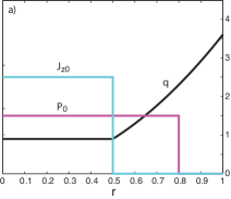
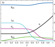
Equilibrium current density $j_{z0}(r),$ pressure $p_{0}(r)$ and safety factor $q(r)$, showing $q=m/n=2/1$, for (a) the stepfunction model used in the analytic studies with $a_{1}=0.5,\,a_{2}=0.8,\,r_{w}=1,\,r_{c}=1.5,\,q(0)=0.9$, and (b) the smooth model used in the numerical studies with $a_{1}=0.55,\,a_{2}=0.7,\,r_{w}=1,\,r_{c}=1.5,\,q(0)=0.8$.

Figure 2:

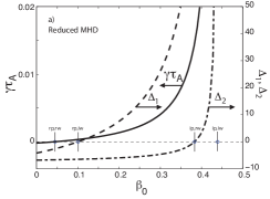
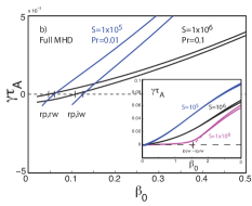
Growth rate $\gamma\tau_{A}$ as a function of $\beta_{0}=2p_{00}/B_{0}^{2}$ for (a) the reduced MHD - stepfunction analytic model with parameters $\tau_{w}=10^{3},\,\tau_{t}=10^{4}$, and (b) the full MHD model with $S=\tau_{R}/\tau_{A}=10^{5}$, $10^{6}$ and $10^{8}$ with both a highly conducting $\tau_{w}=10^{10}$ and transparent $\tau_{w}=0$ wall. In (a) we also show jump quantities $\Delta_{1},\,\Delta_{2}$ as functions of $\beta_{0}$. The four $\beta_{0}$ limits $\beta_{rp,rw}<\beta_{rp,iw}<\beta_{ip,rw}<\beta_{ip,iw}$ marked in (a) are given in Table 1. In (b) the lower limits $\beta_{rp,rw}<\beta_{rp,iw}$ are indicated and change slightly with $S$. The extrapolation to $S=\infty$ is indicated in the inset.

References

- [1] R. Betti and J. P. Freidberg. Stability analysis of resistive wall kink modes in rotating plasmas. Phys. Rev. Letters, 74:2949, 1995.
- [2] S. N. Bhattacharyya. Ideal magnetohydrodynamic stability in the presence of a resistive wall. Phys. Plasmas, 2:4381, 1995.
- [3] J. Bialek, A. H. Boozer, M. E. Mauel, and G. A. Navratil. Modeling of active control of external magnetohydrodynamic instabilities. Phys. Plasmas, 8:2170, 2001.
- [4] C. M. Bishop. An intelligent shell for the reversed field pinch. Plasma Physics and Controlled Fusion, 31:1179–1189, 1989.
- [5] A. Bondeson, Yueqiang Liu, C.M. Fransson, B. Lennartson, C. Breitholtz, and T.S. Taylor. Active feedback stabilization of high beta modes in advanced tokamaks. Nucl. Fusion, 41:455, 2001.
- [6] A. Bondeson and D. Ward. Stabilization of external modes in tokamaks by resistive walls and plasma rotation. Phys. Rev. Letters, 72:2709, 1994.
- [7] A. H. Boozer. Stabilization of resistive wall modes by slow plasma rotation. Phys. Plasmas, 2:4521, 1995.
- [8] M. S. Chu, A. Bondeson, M. S. Chance, Y. Q. Liu, A. M. Garofalo, A. H. Glasser, G. L. Jackson, R. J. La Haye, L. L. Lao, G. A. Navratil, M. Okabayashi, H. Remierdes, J. T. Scoville, and E. J. Strait. Modeling of feedback and rotation stabilization of the resistive wall mode in tokamaks. Phys. Plasmas, 11:2497, 2004.
- [9] M. S. Chu, M. Chance, A. H. Glasser, and M. Okabayashi. Normal mode approach to modelling of feedback stabilization of the resistive wall mode. Nucl. Fusion, 43:441, 2003.
- [10] M. S. Chu, J. M. Greene, T. H. Jensen, R. L. Miller, A. Bondeson, R. W. Johnson, and M. E. Mauel. Effect of toroidal plasma flow and flow shear on global magnetohydrodynamic MHD modes. Phys. Plasmas, 2:2236, 1995.
- [11] J. M. Finn. Resistive wall stabilization of kink and tearing modes. Physics of Plasmas, 2:198, 1995.
- [12] J. M. Finn. Stabilization of ideal plasma resistive wall modes in cylndrical geometry: The effect of resistive layers. Physics of Plasmas, 2:3782, 1995.
- [13] J. M. Finn. Control of resistive wall modes in a cylindrical tokamak with radial and poloidal magnetic field sensors. Phys. Plasmas, 11:4361, 2004.
- [14] J. M. Finn. Control of magnetohydrodynamics modes with a resistive wall above the wall stabilization limit. Phys. Plasmas, 13:082504, 2006.
- [15] J. M. Finn and L. Chacon. Control of linear and nonlinear resistive wall modes. Phys. Plasmas, 11:1866, 2004.
- [16] J. M. Finn and R. A. Gerwin. Mode coupling effects on resistive wall instabilities. Physics of Plasmas, 3:2344, 1996.
- [17] J. M. Finn and R. A. Gerwin. Parallel transport in ideal magnetohydrodynamics and applications to resistive wall modes. Physics of Plasmas, 3:2469, 1996.
- [18] J. M. Finn and W. M. Manheimer. Resistive interchange modes in reversed-field pinches. Phys. Fluids, 25:697, 1982.
- [19] R. Fitzpatrick and A. Aydemir. Stabilization of the resistive shell mode in tokamaks. Nucl. Fusion, 36:11, 1996.
- [20] R. Fitzpatrick and T. Jensen. Stabilization of the resistive wall mode using a fake rotating shell. Physics of Plasmas, 3:2997–3000, 1996.
- [21] H. P. Furth, P. H. Rutherford, and H. Selberg. Tearing mode in the cylindrical tokamak. Phys. Fluids, 16:1054, 1973.
- [22] A. M. Garofalo, T. H. Jensen, L. C. Johnson, R. J. La Haye, G. A. Navratil, M. Okabayayashi, J. T. Scoville, E. J. Strait, D. R. Baker, J. Bialek, and et al. Sustained rotational stabilization of DIII-D plasmas above the no-wall beta limit. Physics of Plasmas, 9:1997, 2002.
- [23] C. G. Gimblett. Stabilization of thin shell modes by a rotating secondary wall. Plasma Phys. Contr. Fusion, 31:2183, 1989.
- [24] A. H. Glasser, J. M. Greene, and J. M. Johnson. Resistive instabilities in a tokamak. Phys. Fluids, 19:567, 1976.
- [25] Y. Q. Liu. Study on resistive wall mode based on plasma response model. Plasma Phys. Control. Fusion, 48:969, 2006.
- [26] Y. Q. Liu and A. Bondeson. Active feedback stabilization of toroidal external modes in tokamaks. Phys. Rev. Letters, 84:907, 2000.
- [27] Y. Q. Liu, A. Bondeson, C. M. Fransson, B. Lennartson, and C. Breitholtz. Feedback stabilization of nonaxisymmetric resistive wall modes in tokamaks. I. Electromagnetic model. Phys. Plasmas, 7:3681, 2000.
- [28] L. Marrelli, P. Zanca, M. Valisa, G. Marchiori, A. Alfier, F. Bonomo, M. Gobbin, P. Piovesan, and et al. Magnetic self organization, MHD active control and confinement in RFX-mod. Plasma Phys. Contr. Fusion, page B359, 2007.
- [29] P. Martin, M.E. Puiatti, P. Agostinetti, M. Agostini, J.A. Alonso, V. Antoni, L. Apolloni, F. Auriemma, F. Avino, A. Barbalace, M. Barbisan, T. Barbui, S. Barison, M. Barp, M. Baruzzo, P. Bettini, M. Bigi, R. Bilel, M. Boldrin, T. Bolzonella, D. Bonfiglio, F. Bonomo, M. Brombin, A. Buffa, C. Bustreo, A. Canton, S. Cappello, D. Carralero, L. Carraro, R. Cavazzana, L. Chacon, B. Chapman, G. Chitarin, G. Ciaccio, W.A. Cooper, S. Dal Bello, M. Dalla Palma, R. Delogu, A. De Lorenzi, G.L. Delzanno, G. De Masi, M. De Muri, J.Q. Dong, D.F. Escande, F. Fantini, A. Fasoli, A. Fassina, F. Fellin, A. Ferro, S. Fiameni, J.M. Finn, C. Finotti, A. Fiorentin, N. Fonnesu, J. Framarin, P. Franz, L. Frassinetti, I. Furno, M. Furno Palumbo, E. Gaio, E. Gazza, F. Ghezzi, L. Giudicotti, F. Gnesotto, M. Gobbin, W.A. Gonzales, L. Grando, S.C. Guo, J.D. Hanson, C. Hidalgo, Y. Hirano, S.P. Hirshman, S. Ide, Y. In, P. Innocente, G.L. Jackson, S. Kiyama, S. F. Liu, Y. Q. Liu, D. Lopez Bruna, R. Lorenzini, T.C. Luce, A. Luchetta, A. Maistrello, G. Manduchi, D.K. Mansfield, G. Marchiori, N. Marconato, D. Marcuzzi, L. Marrelli, S. Martini, G. Matsunaga, E. Martines, G. Mazzitelli, K. McCollam, B. Momo, M. Moresco, S. Munaretto, L. Novello, M. Okabayashi, E. Olofsson, R. Paccagnella, R. Pasqualotto, M. Pavei, S. Peruzzo, A. Pesce, N. Pilan, R. Piovan, P. Piovesan, C. Piron, L. Piron, N. Pomaro, I. Predebon, M. Recchia, V. Rigato, A. Rizzolo, A.L. Roquemore, G. Rostagni, A. Ruzzon, H. Sakakita, R. Sanchez, J.S. Sarff, E. Sartori, F. Sattin, A. Scaggion, P. Scarin, W. Schneider, G. Serianni, P. Sonato, E. Spada, A. Soppelsa, S. Spagnolo, M. Spolaore, D.A. Spong, G. Spizzo, M. Takechi, C. Taliercio, D. Terranova, C. Theiler, V. Toigo, G.L. Trevisan, M. Valente, M. Valisa, P. Veltri, M. Veranda, N. Vianello, F. Villone, Z.R. Wang, R.B. White, X.Y. Xu, P. Zaccaria, A. Zamengo, P. Zanca, B. Zaniol, L. Zanotto, E. Zilli, G. Zollino, and M. Zuin. Overview of the RFX-mod fusion science programme. Nuclear Fusion, 53(10):104018, 2013.
- [30] M. Okabayashi, N. Pomphrey, and R. E. Hatcher. Circuit equation formulation of resistive wall mode feedback stabilization schemes. Nuclear Fusion, 38:1607, 1998.
- [31] L. Piron, L. Marrelli, P. Piovesan, and P. Zanca. Model-based design of multi-mode feedback control in the RFX-mod experiment. Nucl. Fusion, 50:115011, 2010.
- [32] V. D. Pustovitov. Comparison of rwm feedback systems with different input signals. Plasma Phys. Control. Fusion, 44:295, 2002.
- [33] A. S. Richardson, J. M. Finn, and G. L. Delzanno. Control of ideal and resistive magnetohydrodynamic modes in reversed field pinches with a resistive wall. Phys. Plasmas, 17:17, 2010.
- [34] K. Sassenberg, A. S. Richardson, D. P. Brennan, and J. M. Finn. Control of magnetohydrodynamic modes in reversed field pinches with normal and tangential magnetic field sensing and two resistive walls. Plasma Phys. Contr. Fusion, 55:084002, 2013.
- [35] H. R. Strauss. Nonlinear, three-dimensional magnetohydrodynamics of noncircular tokamaks. Phys. Fluids, 19:134, 1976.