18 Sco: a solar twin rich in refractory and neutron-capture elements. Implications for chemical tagging.

Abstract

We study with unprecedented detail the chemical composition and stellar parameters of the solar twin 18 Sco in a strictly differential sense relative to the Sun. Our study is mainly based on high resolution (R $\sim$ 110 000) high S/N (800-1000) VLT UVES spectra, which allow us to achieve a precision of about 0.005 dex in differential abundances. The effective temperature and surface gravity of 18 Sco are $T_{\rm eff}$ = 5823$\pm$6 K and log $g$ = 4.45$\pm$0.02 dex, i.e., 18 Sco is 46$\pm$6 K hotter than the Sun and log $g$ is 0.01$\pm$0.02 dex higher. Its metallicity is [Fe/H] = 0.054$\pm$0.005 dex and its microturbulence velocity is +0.02$\pm$0.01 km s^-1 higher than solar. Our precise stellar parameters and differential isochrone analysis show that 18 Sco has a mass of 1.04$\pm$0.02M_⊙ and that it is $\sim$1.6 Gyr younger than the Sun. We use precise HARPS radial velocities to search for planets, but none were detected. The chemical abundance pattern of 18 Sco displays a clear trend with condensation temperature, showing thus higher abundances of refractories in 18 Sco than in the Sun. Intriguingly, there are enhancements in the neutron-capture elements relative to the Sun. Despite the small element-to-element abundance differences among nearby n-capture elements ($\sim$0.02 dex), we successfully reproduce the $r$- process pattern in the solar system. This is independent evidence for the universality of the $r$-process. Our results have important implications for chemical tagging in our Galaxy and nucleosynthesis in general.

1. Introduction

Solar twins are stars nearly indistinguishable from the Sun (Cayrel de Strobel, 1996). The star 18 Sco was first identified as a solar twin by Porto de Mello & da Silva (1997). This star has great importance because it is the brightest (V = 5.51, Ramírez et al. 2012) and closest (13.9 pc) solar twin (Porto de Mello & da Silva, 1997; Soubiran & Triaud, 2004; Takeda et al., 2007; Datson et al., 2012, 2014; Porto de Mello et al., 2014), thus it can be studied through a variety of techniques. Moreover, 18 Sco has a declination of $-$8 ^∘, hence being observable from both the Northern and Southern hemispheres.

Besides the many recent high resolution chemical abundance studies (e.g. Luck & Heiter, 2005; Meléndez & Ramírez, 2007; Neves et al., 2009; Ramírez et al., 2009a; Takeda & Tajitsu, 2009; González Hernández et al., 2010; da Silva et al., 2012; Monroe et al., 2013), 18 Sco has been observed for chromospheric activity (e.g. Hall et al., 2007), magnetic fields (Petit et al., 2008), debris disks (e.g. Trilling et al., 2008), companions through high resolution imaging (e.g. Tanner et al., 2010), granulation (Ramírez et al., 2009b), seismology (Bazot et al., 2011, 2012) and interferometry (Bazot et al., 2011; Boyajian et al., 2012). In addition, different techniques can be combined to obtain further insights on the fundamental properties of this solar twin (Li et al., 2012).

Most previous abundance studies on 18 Sco report a somewhat enhanced (about 10-15%) iron abundance and a Li content about 3-4 times higher than solar, but otherwise about solar abundance ratios for other elements (e.g. Porto de Mello & da Silva, 1997; Meléndez & Ramírez, 2007; Takeda & Tajitsu, 2009), except for some recent high precision studies on 18 Sco (e.g., Meléndez et al., 2009; Ramírez et al., 2009a; Monroe et al., 2013), which show a clear trend with condensation temperature. The situation regarding the heavy elements is less clear, with Porto de Mello & da Silva (1997) reporting a slight excess in the elements heavier than Sr, but the recent study by Mishenina et al. (2013a) finding about solar ratios for the neutron-capture elements in 18 Sco. Instead, da Silva et al. (2012) found a clear enhancement in Sr, Ba, Nd and Sm, but solar ratios for Y and Ce. To further complicate the situation, González Hernández et al. (2010) found a solar ratio for Nd (an element that was found enhanced by da Silva et al. 2012), but Eu and Zr showed the largest enrichment. The worst cases are Zr and Nd, with a spread of 0.15 dex and 0.14 dex, respectively, and individual values of [Zr/Fe] = -0.05, +0.06, +0.10, and [Nd/Fe] = -0.01, 0.13, 0.00, according to Mishenina et al. (2013a), da Silva et al. (2012) and González Hernández et al. (2010), respectively.

In order to better understand the likely chemical differences between 18 Sco and the Sun, and to clarify the situation regarding the heavy elements (Z $>$ 30), we perform a highly precise abundance analysis of 18 Sco for 38 chemical elements, thus being the most complete and precise abundance study to date on the chemical composition of 18 Sco. Additionally, our precise stellar parameters will be used in a forthcoming paper to better constrain the fundamental properties of 18 Sco in synergy with other techniques such as asteroseismology (Bazot et al., in preparation).

Our work is also relevant regarding “chemical tagging” (Freeman & Bland-Hawthorn, 2002), that aims to reconstruct the build up of our Galaxy by identifying stars with a common origin. Although the dynamical information about their origin could have been lost, the chemical information should be preserved. In this context, the disentangling of the complex abundance pattern of 18 Sco can help us to assess which elements should be targeted for chemical tagging.

The analysis is mainly based on UV-optical spectra acquired with the UVES spectrograph at the VLT and complemented with optical spectra taken with HIRES at Keck.

2. Observations

In order to cover a wide spectral range, we observed 18 Sco and the Sun (using solar reflected light from asteroids) in different spectrograph configurations. Both 18 Sco and the reference solar spectrum were acquired in the same observing runs and using identical setups. We obtained visitor mode observations with the UVES spectrograph at the VLT (August 30, 2009) and with the HIRES spectrograph at Keck (June 16, 2005), covering with both datasets the UV/optical/near-IR spectrum from 306 to 1020 nm.

The UVES observations were taken in dichroic mode, obtaining thus simultaneous UV (blue arm) + optical (red arm) coverage with the standard settings 346 nm + 580 nm, and another set of observations with the standard 346-nm setting plus a non-standard setting centered at 830 nm. With this configuration we achieved a high S/N in the UV, as the 346nm setting (306-387 nm) was covered in both setups. The 580-nm standard setting covered the optical (480 - 682 nm) region and our 830-nm setting included the red region (642 - 1020 nm). Notice that our non-standard setting at 830 nm was chosen to overlap the 580 nm setting in the 642 - 682 nm interval, so that a higher S/N was achieved around 670 nm in order to measure lithium with extremely high precision (e.g., Monroe et al., 2013).

The bulk of the analysis is based on the UVES optical spectra obtained in the red arm covering the 480 - 1020 nm region. The observations with the red arm were obtained using the 0.3 arcsec slit, achieving a high resolving power (R = 110 000) and a very high S/N (typical S/N $\sim$ 800 pixel^-1, and around the Li feature S/N $\sim$ 1000). Some elements showing lines in the UV were studied with the UVES blue arm using the 346 nm setup (306 - 387 nm) with a slit of 0.6 arcsec, resulting in high resolution (R = 65 000) high S/N ($\sim$ 600 at 350 nm) spectra. The asteroid Juno was employed to obtain our reference solar spectrum for the UVES observations, and similar S/N were achieved both for 18 Sco and Juno.

The spectral regions 387-480 nm and 577-585nm are missing in our UVES data, thus, for them we employed high resolution (R = 100 000) high S/N ($\sim$ 400) spectra obtained with the HIRES spectrograph at Keck, that covers the optical spectra (388 - 800 nm) using a mosaic of 3 CCDs. The asteroid Ceres was used to obtain a solar spectrum for our HIRES observations. In Meléndez et al. (2012) we made a detailed comparison of both UVES and HIRES observations of 18 sco relative to the Sun, and concluded that there is an excellent agreement between both datasets, resulting in negligible abundances differences (mean difference of 0.002$\pm$0.001 dex and element-to-element scatter $\sigma$ = 0.005 dex), thus we complement our UVES equivalent width measurements with HIRES data when needed.

Data reductions of the UVES and HIRES spectra are described in Monroe et al. (2013) and Meléndez et al. (2012), respectively. A comparison of the reduced UVES spectra of 18 Sco and the Sun is shown around 6085 Å (Fig. 1) and 5320 Å (Fig. 2). As can be seen in Fig. 1, overall the spectrum of 18 Sco is very similar to the Sun’s, as expected for a solar twin, yet, when a closer look is taken for the lines of neutron-capture elements, a clear enhancement is seen in 18 Sco, as shown for example in Fig. 2 for the 5319.8 Å Nd II line.

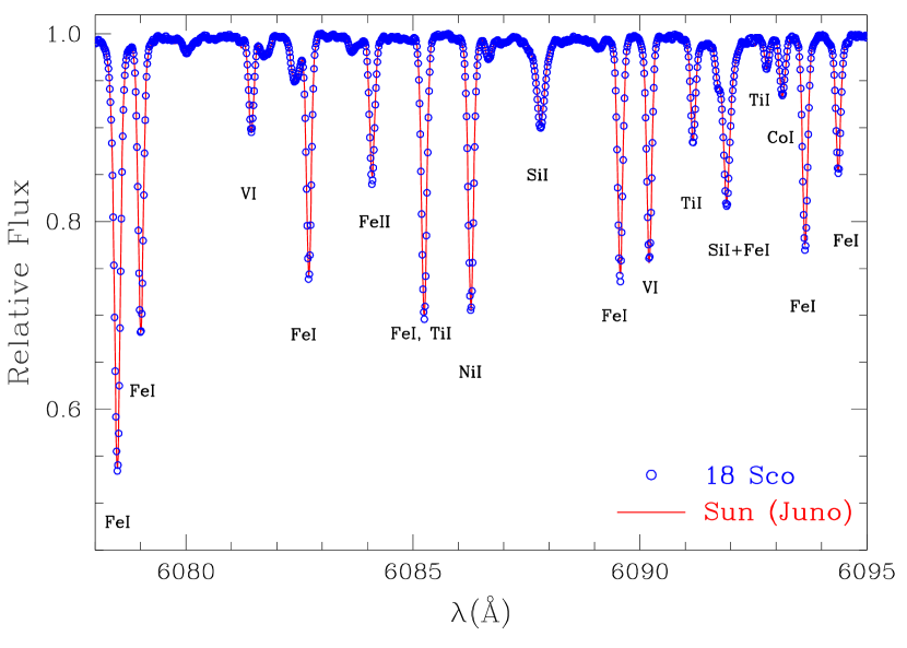
Figure 1.— UVES spectra of 18 Sco and the Sun in the 6078-6095 Å region. Albeit both stars show similar spectra, their different chemical compositions can be revealed through careful measurements.

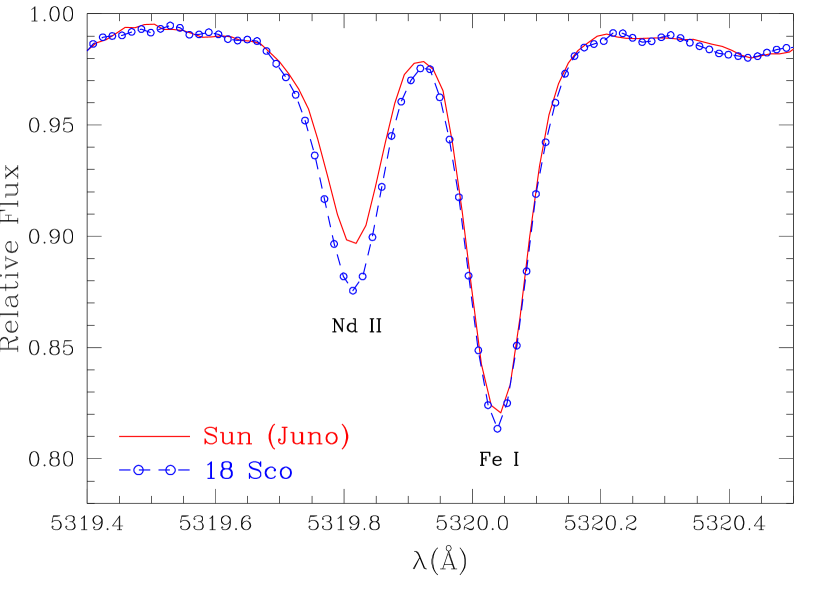
Figure 2.— UVES spectra of 18 Sco and the Sun around 5320 Å, showing a clear enhancement in the n-capture element Nd in 18 Sco, relative to the Sun.

3. Abundance analysis

The abundance analysis closely follows our recent high precision studies on the solar twins HIP 56948 (Meléndez et al., 2012) and HIP 102152 (Monroe et al., 2013). We measured the equivalent widths (EW) automatically with ARES (Sousa et al., 2007) for lines with EW larger than 10 mÅ. Weaker lines, as well as species with less than 5 lines available, were measured by hand using IRAF. In further iterations the outliers resulting from the automatic EW measurements are carefully measured by hand, making sure that exactly the same criteria are used in the measurements of 18 Sco and the Sun, i.e., for each line we choose the same continuum definition and the same interval was selected to fit a gaussian profile. The main difference in relation to Meléndez et al. (2012) and Monroe et al. (2013), is that we have significantly expanded our line list to obtain more precise results and also to include many heavy elements. For example, in Meléndez et al. (2012) only 54 iron (42 Fe I, 12 Fe II) and 12 chromium (7 Cr I, 5 Cr II) lines were included, while in the present work 98 iron (86 Fe I, 12 Fe II) and 21 chromium (14 Cr I, 7 Cr II) lines are used. In comparison to Monroe et al. (2013), we have 87 additional lines, many of which were included to study the neutron-capture elements.

Since our abundances were estimated from EW, we selected mostly clean lines. For example, the oxygen abundance was estimated using the clean O I triplet at 777nm rather than the blended forbidden [O I] line at 630nm. When necessary we used lines somewhat affected by blending, measuring them by using multiple gaussians with the deblend option of the task splot in IRAF. The list of lines with the differential equivalent width measurements is presented in Table LABEL:EW, except for nitrogen and lithium, that were analysed by spectral synthesis of a NH feature at 340nm and the Li I feature at 670.7nm, respectively.

We obtain both stellar parameters and elemental abundances through a differential line-by-line analysis (e.g., Meléndez et al., 2012; Monroe et al., 2013; Ramírez et al., 2011; Ramírez et al., 2014a), using Kurucz ODFNEW model atmospheres (Castelli & Kurucz, 2004) and the 2002 version of MOOG (Sneden, 1973). For the Sun we fixed $T_{\rm eff}$ = 5777 K and log $g$ = 4.44 (Cox, 2000) and as initial guess we used a microturbulence velocity of v_t = 0.86 km s^-1 (Monroe et al., 2013). Solar abundances were then computed and the final solar microturbulence was found by imposing no trend between the abundances of Fe I lines and reduced equivalent width (EW_r = EW/$\lambda$). We found v${}_{t}^{\odot}$ = 0.88 km s^-1 and used this value and the above $T_{\rm eff}$ and log $g$ to compute the reference solar abundances ($A_{i}^{\odot}$).

Next, adopting as initial guess for 18 Sco the solar stellar parameters, we computed abundances for 18 Sco ($A_{i}^{*}$), and then differential abundances for each line $i$,

$$\delta A_{i}=A_{i}^{*}-A_{i}^{\odot}.$$ (1)

The effective temperature is found by imposing the differential excitation equilibrium of $\delta A_{i}$ for Fe I lines:

$$d(\delta A_{i}^{\rm FeI})/d(\chi_{\rm exc})=0,$$ (2)

while the differential ionization equilibrium of Fe I and Fe II lines was used to determine the surface gravity:

$$<\delta A_{i}^{\rm FeII}>-<\delta A_{i}^{\rm FeI}>\;=\;0.$$ (3)

The microturbulence velocity, v_t, was obtained when the differential Fe I abundances $\delta A_{i}^{\rm FeI}$ showed no dependence with the logarithm of the reduced equivalent width:

$$d(\delta A_{i}^{\rm FeI})/d(\log_{10}(EW_{r}))=0.$$ (4)

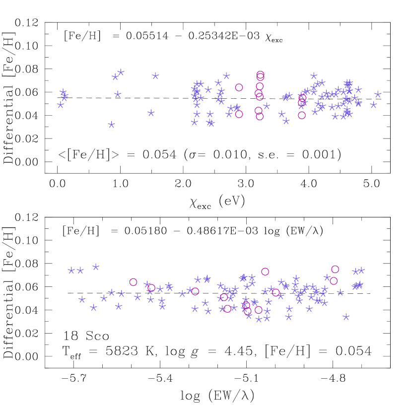
Figure 3.— Differential iron abundances versus excitation potential (top panel) and reduced equivalent width (bottom panel) of Fe I (stars) and Fe II (circles) lines. The dashed lines show fits to the Fe I lines. The solution is achieved when the slopes are equal or smaller than one third of the error bar in the slopes, and when the mean abundance of Fe II agrees with the mean abundance of Fe I within one third of the combined error bar.

The spectroscopic solution is reached when the three conditions above (eqs. 2-4) are satisfied simultaneously to better than $\sim$1/3 the error bars in the slopes of eqs. 2 and 4, and better than $\sim$1/3 of the error bar of the quadratic sum of the error bars of Fe I and Fe II lines for eq. 3. We preferred to adopt these convergence criteria based on the observational error bars rather than using fixed values. Also, the metallicity obtained from the iron lines must be the same as that of the input model atmosphere (within 0.01 dex).

We emphasise that our iron line list was built to minimize potential correlations between the atmospheric parameters, by including lines of different line strengths at a given excitation potential, and by having, inasmuch as possible, a homogeneous distribution of lines with excitation potential. Besides, we keep in our line list only iron lines that could be reliably measured at high precision at our spectral resolution.

The differential spectroscopic equilibrium (Fig. 3) results in the following stellar parameters: $T_{\rm eff}$ = 5823$\pm$6 K (46$\pm$6 K hotter than the Sun), log $g$ = 4.45$\pm$0.02 dex (+0.01$\pm$0.02 dex above the Sun), [Fe/H] = 0.054$\pm$0.005 dex, and $\Delta v_{t}$=+0.02$\pm$0.01 km s^-1 higher than solar. The above errors include both the measurement uncertainties (from the errors in the slopes and the errors in the iron abundances), and the degeneracies in the stellar parameters, by estimating how the error in a given stellar parameter affects the uncertainty in the others. For example, besides the uncertainty in log $g$ due to the errors in Fe I and Fe II, we estimated systematic errors in log $g$ due to changes in Fe II - Fe I owing to the uncertainties in $T_{\rm eff}$, $v_{t}$ and [Fe/H].

In Meléndez et al. (2012) we found that the small differential NLTE corrections to Fe I lines in the solar twin HIP 56948 do not affect the excitation temperature derived in LTE. Here we also computed NLTE corrections for Fe I as in Bergemann et al. (2012). Again, the differential NLTE corrections are so small that they do not have any impact on our spectroscopic solution. Notice that, within the error bars, the differential ionization equilibrium is satisfied also by Cr, Ti and Sc, as shown in Fig. 4. This good agreement among different species reinforces our results.

Figure 4.— Singly-ionized minus neutral differential abundances of Fe, Cr, Ti and Sc. The surface gravity found by the ionization equilibrium of iron also satisfies, within the error bars, the ionization equilibrium of Sc, Ti and Cr.

Our stellar parameters are in excellent agreement with those independently determined by Monroe et al. (2013), who found a $T_{\rm eff}$ only 1 K hotter, exactly the same log $g$ and $v_{t}$ and [Fe/H] only 0.001 dex higher, and by Takeda & Tajitsu (2009), who determined $T_{\rm eff}$ = 5826$\pm$5 K, log $g$ = 4.45$\pm$0.01 dex, and [Fe/H] = 0.06$\pm$0.01 dex, using high resolution ($R$ = 90 000) high S/N ($\sim$1000 at 600 nm) HDS/Subaru spectra. Our results are also in firm agreement with stellar parameters recently determined by Ramírez et al. (2014b) using several high resolution (R = 65000 - 83 000) high S/N (= 400) spectra taken with the MIKE spectrograph at the Magellan telescope, $T_{\rm eff}$ = 5816$\pm$4 K, log $g$ = 4.45$\pm$0.01 dex, and [Fe/H] = 0.053$\pm$0.003. Also, there is a good agreement with other results found in the literature, as well as an exceptional accord with their weighted mean value, $T_{\rm eff}$ = 5822$\pm$4 K, log $g$ = 4.45$\pm$0.01 dex, and [Fe/H] = 0.053$\pm$0.004, as shown in Table 2.

We took hyperfine structure (HFS) into account for 11 elements. The calculation is performed including HFS for each individual line and then a differential line-by-line analysis is performed. Also, isotopic splitting was taken into account for the heavier elements. For V, Mn, Ag, Ba, La, Pr the combined HFS+isotopic splitting is a minor differential correction ($\leq$ 0.002 dex), but for Co and Cu the differential correction amounts to 0.004 dex, for Y the correction is 0.005 dex, and for Yb it is very large at 0.023 dex. The most dramatic case is for Eu, for which neglecting the corrections would result in an error of 0.155 dex in the differential abundances.

As shown in Meléndez et al. (2012) and Monroe et al. (2013), differential NLTE effects in solar twins relative to the Sun are minor. Here, we consider differential NLTE corrections for elements showing the largest differential corrections in our previous works, Mn (Bergemann & Gehren, 2008) and Cr (Bergemann & Cescutti, 2010), but the largest differential correction is only 0.003 dex for Mn. As mentioned above, differential NLTE effects on Fe (Bergemann et al., 2012) were also estimated to check for potential systematics in our differential stellar parameters, but there is no impact in our solutions.

Our differential abundances (which are based on EW measured by J. Meléndez) are in excellent agreement with those obtained using an independent set of EW measurements in 18 Sco by Monroe et al. (2013), with an average difference of 0.002 dex (this work - Monroe et al.) and an element-to-element scatter of only 0.005 dex. Another independent set of EW measurements obtained by M. Tucci Maia (that were obtained fully by hand, unlike the measurements done by J.M and T.M., which used ARES first and then re-measured the outliers by hand), results in abundances with a difference from our work of 0.002 dex and scatter of only 0.004 dex. These comparisons, and our previous testing in Meléndez et al. (2012), for which we obtained an element-to-element scatter of $\sigma$ =0.005 dex, in the similarity of HIRES and UVES abundances of 18 Sco minus the Sun, suggest that careful differential measurements can achieve a precision of about 0.005 dex in differential abundances.

The measurement errors are adopted as the standard error of the differential abundances, except for elements with just a single line, in which case we adopted as observational error the standard deviation of five differential EW measurements performed with somewhat different criteria. The typical measurement uncertainties in the differential abundances of the lighter elements (Z $\leq$ 30) are about 0.004 dex, in good agreement with the measurement errors discussed above. Including the systematic errors due to uncertainties in the stellar parameters, the total error is about 0.007 dex. The differential abundances for each element and their errors are given in Table 3.

4. Mass, age, rotation and lithium

We determine the mass and age of 18 Sco using our precise stellar parameters ($T_{\rm eff}$ = 5823$\pm$6 K, log $g$ = 4.45$\pm$0.02 dex, [Fe/H] = 0.054$\pm$0.005 dex) and Yonsei-Yale isochrones (Yi et al., 2001; Kim et al., 2002; Demarque et al., 2004). The method, which uses the stellar parameters, their error bars, and probability distribution functions, is described in detail in Meléndez et al. (2012) and Chanamé & Ramírez (2012). The method was calibrated to reproduce the solar values, as described in Meléndez et al. (2012).

We obtain an age of 2.9${}_{-1.0}^{+1.1}$ Gyr for 18 Sco, i.e., 1.6 Gyr younger than the Sun, for which we derived an age of 4.5 Gyr using the same set of isochrones (Meléndez et al., 2012). Stellar ages can be well-constrained from isochrones, provided that stellar parameters are known with extreme precision, as shown in Fig. 5a, where we compare our stellar parameters and error bars to the Yonsei-Yale isochrones. We show in Fig. 5b that Padova isochrones (Bressan et al., 2012) are compatible with the relative ages between the Sun and 18 Sco obtained from Yonsei-Yale isochrones. Our age agrees well with the value found by do Nascimento et al. (2009), 2.89${}_{-0.81}^{+1.09}$ Gyr, using lithium abundances and stellar parameters. Within the error bars, our age also agrees with that determined by Li et al. (2012), 3.66${}_{-0.50}^{+0.44}$ Gyr, using different constraints (stellar parameters, lithium abundance, rotation and average large frequency separation). Notice, however, that the adopted stellar parameters by Li et al. (2012) are not as precise as those reported in this work. We are currently modeling our HARPS seismic observations of 18 Sco to obtain even better constraints on its age.

Following Meléndez et al. (2012), we obtain $v$ sin $i_{\rm 18Sco}$/$v$ sin $i_{\odot}$ = 1.069$\pm$0.029. Adopting $v$ sin $i_{\odot}$ = 1.90 km s^-1 for the Sun (Bruning, 1984; Saar & Osten, 1997), this implies $v$ sin $i_{\rm 18Sco}$ = 2.03$\pm$0.05 km s^-1. The higher rotation rate in 18 Sco is compatible with its younger age. Fortunately, the rotation period has been determined for this star, $P$ = 22.7$\pm$0.5 days (Petit et al., 2008), resulting in a rotational age of 3.36$\pm$0.52 Gyr using the rotation-age relationship given in Barnes (2007). This value is in good agreement with our derived isochronal age (2.9${}_{-1.0}^{+1.1}$ Gyr).

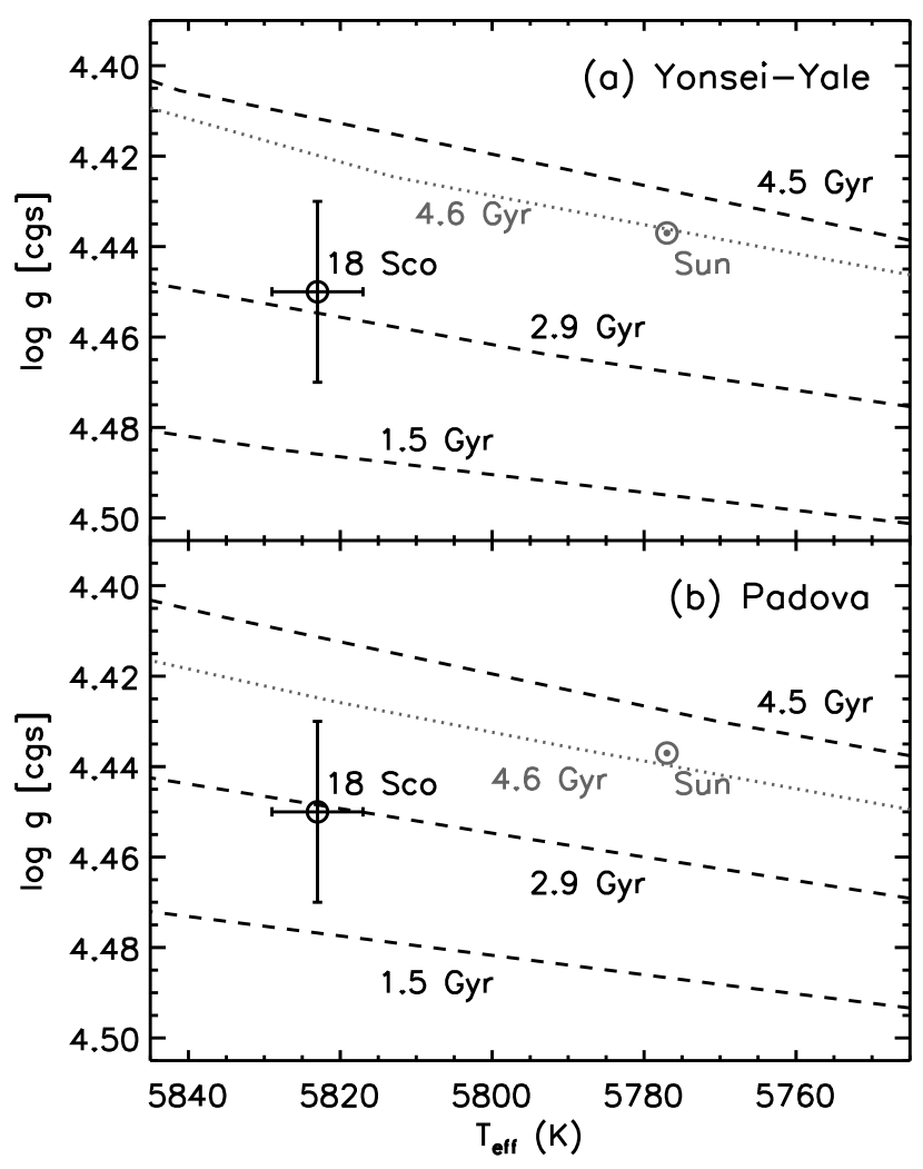
Figure 5.— Location of the Sun and 18 Sco on the HR diagram. (a): Yonsei-Yale isochrones of [Fe/H]=+0.05 (the metallicity of 18 Sco) and age=1.5, 2.9, and 4.5 Gyr are shown (dashed lines) along with a solar metallicity isochrone of solar age (dotted line). The high precision of our derived stellar parameters for 18 Sco allows us to infer a reasonable estimate of its age from the theoretical isochrones, even though they are densely packed in this main-sequence region. (b): as above for Padova isochrones, showing consistent results for the relative ages between 18 Sco and the Sun.

The mass derived here is 1.04$\pm$0.02 M_⊙, which agrees well with the detailed study of Li et al. (2012), who reported 1.045 M_⊙ using isochrones, 1.030 M_⊙ adding also lithium, and 1.030, including stellar parameters, lithium and the mean large frequency separation. The mass derived by do Nascimento et al. (2009), 1.01$\pm$0.01 M_⊙, is also in agreement with our results within the error bars, as well as with the mass derived using asteroseismology, 1.02$\pm$0.03 M_⊙ (Bazot et al., 2011) and 1.01$\pm$0.03 M_⊙ (Bazot et al., 2012). We are performing a more detailed seismic analysis of 18 Sco including also new HARPS observations (Bazot et al., in preparation).

The Li abundance (A${}_{\rm Li}^{\rm NLTE}$ = 1.62 $\pm$ 0.02 dex) was derived using the line list presented in Meléndez et al. (2012) and NLTE corrections by Lind et al. (2009), and is identical to that obtained by Monroe et al. (2013), as the stellar parameters are essentially the same, except for a 1 K difference in the effective temperature. We refer the reader to Monroe et al. (2013) for further details, but we stress here that our Li abundance fits well the trend of Li depletion with age of several non-standard solar models (e.g., Charbonnel & Talon, 2005; do Nascimento et al., 2009; Xiong & Deng, 2009; Denissenkov, 2010).

5. Companions around 18 Sco

18 Sco is included in our HARPS Large Program to search for planets around solar twins, hence we can evaluate whether planets or a binary component are present.

Radial velocities were obtained with the HARPS instrument and binned to yield one RV value per night for a total of 59 nights spanning from May 2004 to February 2014. The observations include 20 nights of high-cadence asteroseismic observations without simultaneous reference in addition to 39 nights of observations with simultaneous ThAr reference for instrumental drift correction. The asteroseismic data have a scatter of 1 m s^-1 throughout the course of a single night. When a moving average is applied to smooth out random noise, a coherent and repeated nightly pattern with an amplitude on order of 2 m s^-1 emerges. We conclude that this coherent noise may be instrumental in origin and minimize its effect on the data by using only a single data point from each night obtained by a weighted average of points from the 4 hours with lowest airmass. Additionally, the radial velocities show drifts throughout the course of the two asteroseismic observing runs which may be instrumental or, in the case of the May 2012 observations, may be a signal from starspots. We make no attempt to remove these drifts due to the uncertainty of their origin.

Activity indices were also calculated for each HARPS spectrum from the Ca II H & K lines. The activity cycle of 18 Sco is present in the data, with radial velocities increasing at times of high activity as photospheric convection is suppressed. This variation occurs on a timescale of 7.6 years in the data, consistent with the previously measured period of seven years from photometry and chromospheric activity (Hall et al., 2007). We remove the effect of the activity cycle on the RVs by fitting and subtracting a linear correlation between radial velocity and continuum-normalized Ca II H & K flux ($S_{HK}$).

The resulting radial velocity measurements were searched for planet signals with no significant detections. We quantify our upper limits on potential planets as follows. We make a flat-line fit to the data and subtract the offset. We then fold all jitter in the radial velocities into the uncertainties on the residuals by scaling them with the reduced chi-squared of the fit. The residuals are resampled randomly with replacement, and a Keplerian signal of fixed planet period and mass is added. If the resulting simulated RVs are inconsistent with a flat-line fit by three or more sigma for 99% of randomized trials at a given planet period and mass, we consider the planet to be excluded by the data. The resulting exclusion limits rule out sub-Neptune-mass objects out to a period of 7 days, and Jupiter-mass objects out to approximately 13 years (Fig. 6). As with all ground-based radial velocity observations, these data show aliases on timescales around 1 day (due to observing nightly), and at approximately 30 and 365 days due to the effects of the lunar cycle and seasonal observability on sampling.

Our HARPS RV measurements also exclude the presence of a binary component, which is consistent with no detection of companions around 18 Sco by high-contrast AO imaging (Tanner et al., 2010).

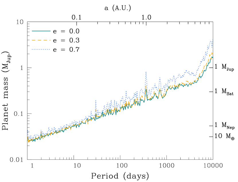
Figure 6.— Detection limits based on our HARPS data are shown for different eccentricities (e) as a function of orbital period. Planets above the curves are ruled out.

6. The complex abundance pattern of 18 Sco

As can be seen in Fig. 7, 18 Sco presents a complex abundance pattern. On top of the typical trend with condensation temperature seen in other solar twins (Meléndez et al., 2009; Ramírez et al., 2009a, 2010), corresponding in Fig. 7 to the group of elements with enhancements [X/H] $\leq$ 0.06 dex (filled circles), there is a group of elements with much larger enhancements (0.09 $<$ [X/H] $<$ 0.19 dex; filled triangles). All elements in the latter group are neutron-capture elements.

In order to understand the large enhancement of the n-capture elements in 18 Sco, we first need to subtract the trend with condensation temperature, as it is probably related to the deficiency of refractory elements in the Sun (Meléndez et al., 2009); besides, the yields of AGB stars and SN do not produce such a trend (Meléndez et al., 2012). We fit [X/H] vs. condensation temperature (Lodders, 2003) for the lighter elements with Z $\leq$ 30, because they only seem affected by the condensation temperature. The fit (Fig. 8) results in:

$$[X/H](Z\leq 30)=-0.005+3.485\times 10^{-5}T_{\rm cond},$$ (5)

with an element-to-element scatter of only 0.008 dex, which is similar to the mean total error (0.007 dex) of our differential abundances for elements with Z $\leq$ 30 (Table 3), showing thus that our small error bars are realistic. The significance of the slope is 9 $\sigma$.

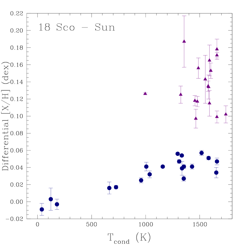
Figure 7.— Differential abundances of 18 Sco relative to the Sun. Elements with [X/H] $\leq$ 0.06 (filled circles) have Z $\leq$ 30, i.e, Zinc and lighter elements, while the elements with [X/H] $>$ 0.09 (filled triangles) have Z $>$ 30.

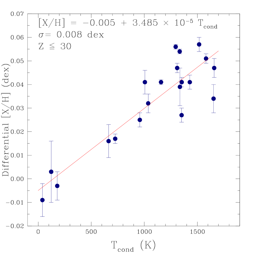
Figure 8.— Fit of the trend with condensation temperature for elements with Z $\leq$ 30. The slope has a significance of 9 $\sigma$ and the element-to-element scatter from the fit is only 0.008 dex.

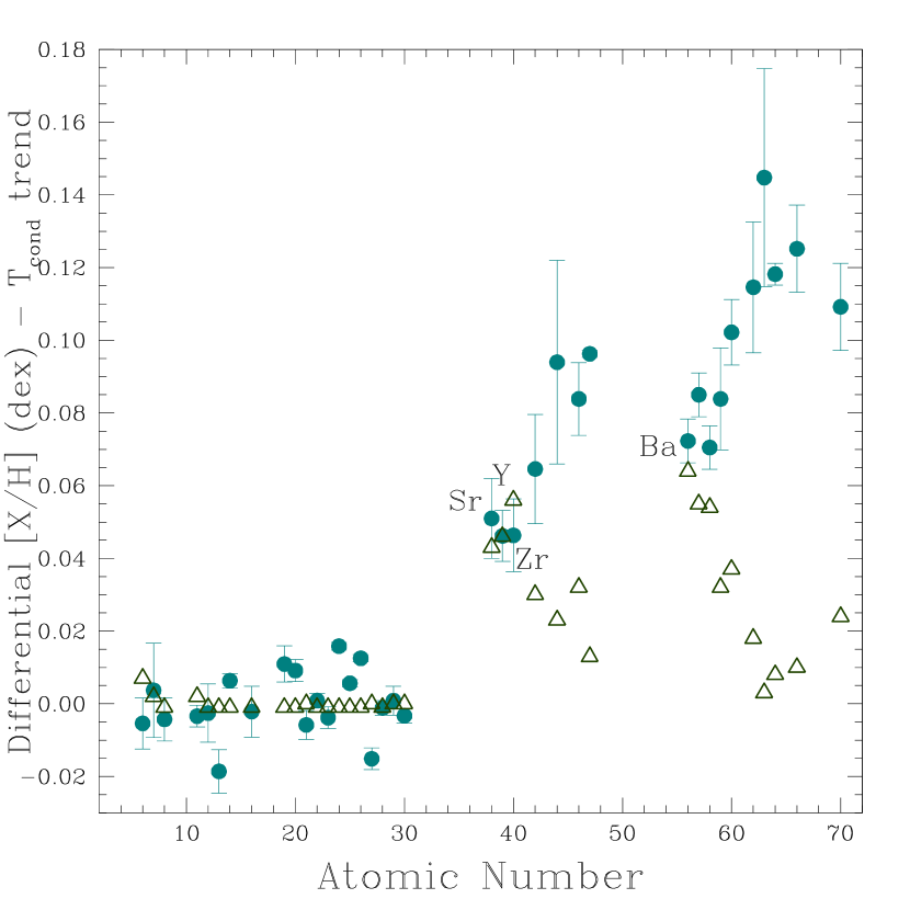
Figure 9.— The filled circles are the [X/H] ratios in 18 Sco after they have been subtracted from the condensation temperature trend shown in Fig. 8. Elements with Z $\leq$ 30 now have abundance ratios close to zero but the neutron-capture elements remain enhanced. The open triangles represent the effect of pollution by an AGB star (see the text for details). Although a good match can be seen for the s-process elements Sr, Y, Zr and Ba, there is a disagreement for other elements.

Next, we subtract the above trend from the [X/H] abundances:

$$[X/H]_{T}=[X/H]-(-0.005+3.485\times 10^{-5}T_{\rm cond}).$$ (6)

The [X/H]_T ratios are given in Table 4 and are shown by filled circles in Fig. 9.

We first verify if the observed enhancement in the n-capture elements is due to pollution by AGB stars. We used a model of a 3 M_⊙ AGB star of Z = 0.01 (Karakas, 2010) and diluted the yields of a small fraction of AGB ejecta ($\leq$ 1% of material injected) into a 1 M_⊙ proto cloud of solar composition (Asplund et al., 2009). Then, we computed the enhancement in the abundance ratios relative to the initial composition of the proto cloud, [X/H]_AGB. A dilution of 0.23% mass of AGB material matched the observed enhancement in the light $s$-process element yttrium. The [X/H]_AGB ratios are given in Table 4 and shown by open triangles in Fig. 9. As can be seen, a good match cannot be achieved for all the n-capture elements, showing that there is an additional source for the abundance enhancement. Nevertheless, other $s$-process elements besides Y, such as Sr, Zr and Ba are well fitted, thus, the observed enhancement could be due, at least partly, to AGB stars. In order to find out if the residual enhancement is due to the $r$-process, we estimated its enrichment in 18 Sco by subtracting the AGB contribution

$$[X/H]_{r}=[X/H]_{T}-[X/H]_{\rm AGB},$$ (7)

and compare these results with the predicted enhancement based on the $r$-process fractions in the solar system, $r_{SS}=1-s_{SS}$, using the $s$-fractions ($s_{SS}$) by Simmerer et al. (2004) and Bisterzo et al. (2011, updated for a few elements by Bisterzo et al. 2013). Then, we can estimate the $r$-process contribution [X/H]${}_{r}^{SS}$ from

$$1-s_{SS}=10^{[X/H]_{r}^{SS}/\Delta_{T}}/10^{[X/H]_{T}/\Delta_{T}},$$ (8)

where we define $\Delta_{T}$ as the average of the three most enhanced $s$-process and $r$-process elements, corresponding to $\Delta_{T}$ = 0.093 dex for the observed [X/H]_T enrichment in 18 Sco (Table 4).

Therefore, the predicted $r$-process contribution based on the solar system $r$-fractions, [X/H]${}_{r}^{SS}$, is:

$$[X/H]_{r}^{SS}=\Delta_{T}\times\log_{10}(1-s_{SS})+[X/H]_{T}.$$ (9)

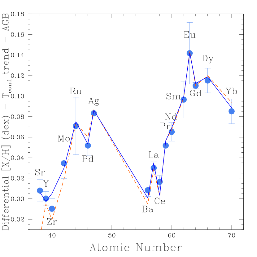
Figure 10.— The filled circles represent the [X/H] ratios in 18 Sco after they have been subtracted from the condensation temperature trend (Fig. 8) and from the AGB contribution (Fig. 9). The residual enhancement, [X/H]_r (filled circles), is in extraordinary agreement with the predicted $r$-process enhancement based on the solar system $r$-process fractions by Simmerer et al. (2004) and Bisterzo et al. (2011, 2013), represented by dashed and solid lines, respectively.

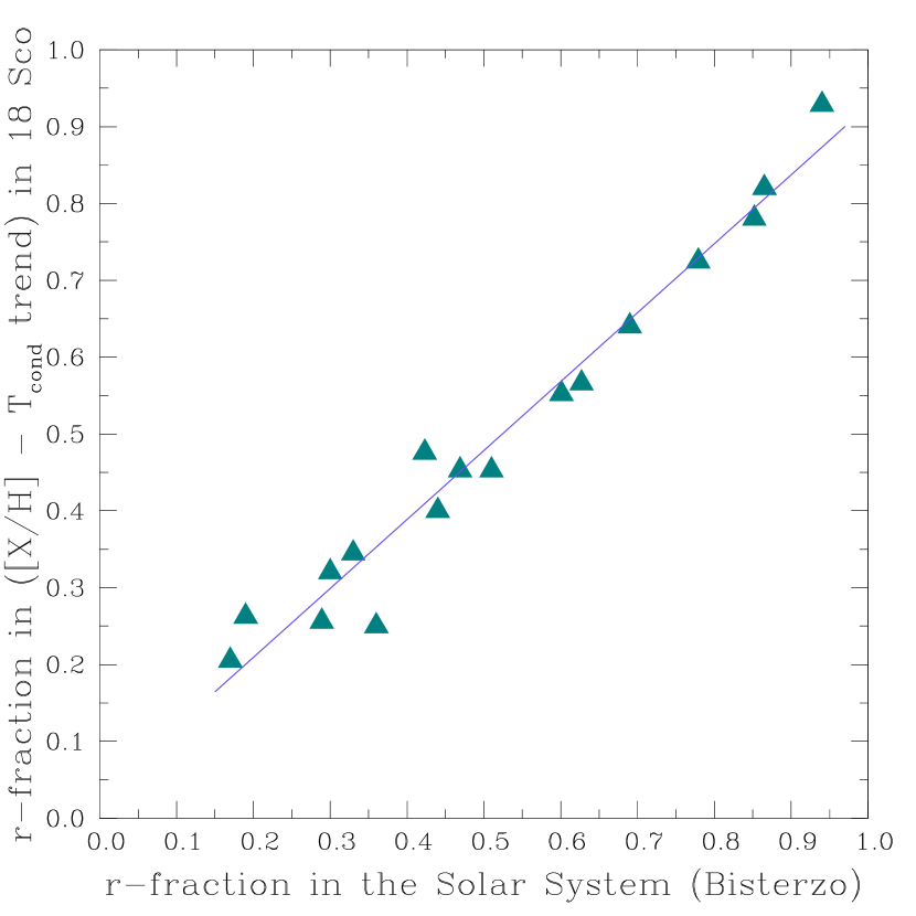
Figure 11.— The $r$-process fractions in the [X/H]_T abundance ratios in 18 Sco versus the $r$-fractions in the solar system (Bisterzo et al., 2011, 2013). The line shows a linear fit with slope of 0.90 and element-to-element scatter of only 0.04.

In Fig. 10, we compare the “observed” $r$-process enhancement [X/H]_r (eq. 7) with the predicted one based on the solar system $r$-process fractions, [X/H]${}_{r}^{SS}$ (eq. 9). There is an astonishing agreement, strongly suggesting that the remaining enhancement is indeed due to the $r$-process. The impressive agreement, even at the scale of the small fluctuations ($\sim$0.02 dex) among nearby n-capture elements (Fig 10), also suggests that even for heavy elements we suceeded in achieving abundances with errors of about 0.01 dex.

Another way to show that the residual enhancement (after subtracting the AGB contribution) is due to the $r$-process, is by comparing the $r$-fractions of the [X/H]_T ratios with the $r$-fractions in the solar system. Since the Bisterzo et al. (2011, 2013) $s_{SS}$-fractions fit somewhat better our [X/H]_r ratios (Fig. 10), we will use their values in the comparison. The “observed” $r$-fractions in the [X/H]_T ratios in 18 Sco, are estimated by

$$r=10^{[X/H]_{r}/\Delta_{T}}/10^{[X/H]_{T}/\Delta_{T}}.$$ (10)

The “observed” $r$-fractions and the solar system $r_{SS}$-fractions (Bisterzo et al., 2011, 2013), are compared in Fig. 11. Again, the agreement is remarkable (slope of 0.90 and element-to-element scattter of only 0.04), showing that after both the T_cond trend and AGB contribution are subtracted, the remaining material can be explained by the $r$-process. Our high precision abundances provide independent evidence of the universality of the $r$-process, i.e., to the remarkable similarity of the relative abundance pattern among different $r$-process elements. Our finding is similar to what is found in metal-poor stars, where the scaled solar $r$-process pattern match the abundances of most neutron-capture elements (e.g., Cowan et al., 2002; Hill et al., 2002; Frebel et al., 2007; Sneden et al., 2008; Siqueira Mello et al., 2013).

The complex abundance pattern of 18 Sco can be thus explained by the condensation temperature trend, the $s$-process and the $r$-process. The excess of refractory elements relative to the Sun seems to be typical of solar like stars (Meléndez et al., 2009; Ramírez et al., 2009a, 2010; Schuler et al., 2011; Liu et al., 2014; Mack et al., 2014), so 18 Sco looks normal in this regard. As we will see below, the additional enhancement in the n-capture elements may be explained by the younger age of 18 Sco (Section 4).

A deficiency in the abundances of the $s$-process elements have been reported in our analysis of the pair of almost solar twins 16 Cyg (Ramírez et al., 2011) and the solar twin HIP 102152 (Monroe et al., 2013), which are both older than the Sun by 2.5 and 3.7 Gyr, respectively. On the contrary, the s-process elements seem enhanced in the young solar twin 18 Sco. Thus, the increasing enhancement of the $s$-process elements with decreasing age is probably due to the pollution of successive generations of AGB stars, that can be tracked using solar twins spanning ages from 2.9 Gyr (18 Sco) up to 8.2 Gyr (HIP 102152). Similar enhancements of the s-process elements have been found in open clusters (e.g., D’Orazi et al., 2009; Maiorca et al., 2011; Yong et al., 2012; Jacobson & Friel, 2013; Mishenina et al., 2013b), with Ba showing the clearest trend of increasing abundance for younger ages. A similar trend was observed in field stars (Edvardsson et al., 1993; Bensby et al., 2007; da Silva et al., 2012), but Mishenina et al. (2013a) found no dependence of [Ba/Fe] and [La/Fe] with age. Albeit there is no consensus yet, most evidences point out for enhanced $s$-process abundances for decreasing ages.

Regarding the r-process elements, da Silva et al. (2012) found a decrease of [Sm/Fe] for decreasing ages in stars younger than the Sun. Using both Eu abundances (4129 Å line) and stellar ages determined by Bensby et al. (2005) in thin disk stars, we found that for ages lower than 9 Gyr there is a flat [Eu/Fe] ratio, i.e., no dependence with stellar age. Unfortunately, neither del Peloso et al. (2005) nor Mishenina et al. (2013a) studied the dependence of their [Eu/Fe] ratios with age in thin disk stars. Our analysis of two old solar twins (Ramírez et al., 2011; Monroe et al., 2013), found normal $r$-process abundances for 16 Cyg B and HIP 102152. Based on the limited evidence, $r$-process elements seem to have a flat behavior with age.

Since 18 Sco is considerably younger than the Sun, the enhancement in the $s$-process elements could be due just to normal Galactic chemical evolution. However, the enhancement of the $r$-process elements in 18 Sco is more difficult to understand, as, based on our discussion above, those elements are not expected to be enriched.

The unexpected enhancement of the $r$-process elements in 18 Sco could be attributed to a somewhat higher contribution of $r$-process ejecta to the natal cloud of 18 Sco than around other solar-like stars.

Our precise abundances show that whatever sources that produced the enrichment in the n-capture elements, did not produce substantial quantities of elements lighter than Z = 30. The amount of mass with Z $>$ 30 that would be needed to produced the observed enhancements is very small, only 2.7 $\times 10^{-8}$ M_⊙ and 2.4 $\times 10^{-7}$ M_⊙ for the $s$- and $r$-process, respectively.

7. Implications for Chemical Tagging

Studying the detailed abundance pattern of solar type stars we may be able to reconstruct the build up of the Galaxy using chemical tagging (Freeman & Bland-Hawthorn, 2002). One of the main problems when tagging individual stars to a given natal cloud may be radial migration (Sellwood & Binney, 2002), yet the chemical abundances may be preserved, hence using chemical tagging stellar groups or clusters could be reconstructed.

Based on our precise abundances in 18 Sco, it is clear that different elements should be targeted for chemical tagging. First, as many of the highly volatile (C, N, O) and highly refractory elements (Al, Ti, Sc, Ca, V, Fe) should be analyzed to determine if there is any trend with condensation temperature. If possible it would be important to cover also some semi-volatiles (e.g., S, Zn, Na, Cu, K, Mn, P) and some medium refractories (e.g., Si, Mg, Cr, Ni, Co, V), to verify if there is a break in the trend with condensation temperature (Meléndez et al., 2009). Also, it should be important not to discard stars from a given group due to small discrepant abundances, as those anomalies could be due to either the formation of terrestrial (Meléndez et al., 2009) or giant (Tucci Maia et al., 2014; Ramírez et al., 2011) planets.

Some of the above elements are of course relevant to different nucleosynthetic processes such as production of $\alpha$ elements (O, S, Ca, Si, Ti) by SNe II or signatures of proton-burning (Na, Mg, Al, O). Li is important as a potential chronometer (Baumann et al., 2010; Monroe et al., 2013; Melendez et al., 2014) and to study the transport mechanisms inside stars (e.g. Charbonnel & Talon, 2005; do Nascimento et al., 2009). The study of 18 Sco also shows the importance of including the heavy elements for chemical tagging. Ideally, at least some elements between Sr, Zr, Y or Ba should be included to verify the $s$-process and some elements among Ru, Pd, Ag, Sm, Gd, Eu or Dy could be explored for the $r$-process.

8. Conclusions

We have performed the most precise and complete abundance analysis of 18 Sco. Being the brightest of the solar twins, very high S/N, high resolution spectra were gathered for 18 Sco and the Sun and a strictly differential line-by-line analysis was performed allowing us to achieve a precision of about 0.005 dex in differential abundances. Additionally, highly precise stellar parameters were obtained, which would be important for further modeling of this solar twin using different techniques. Precise radial velocities were gathered with HARPS, but no planet has been detected yet.

The complex abundance pattern of 18 Sco shows enhancements (relative to the Sun) in the refractory, $s$-process and $r$-process elements. After subtracting the trend with condensation temperature and the contribution from AGB stars, the remaining enhancement shows the same pattern as the $r$-process in the solar system. This shows the universality of the $r$-process. The different contributions to the abundance enrichment in 18 Sco could be disentangled thanks to the exquisite precision achieved in our work.

18 Sco serves as a testbed for studies of chemical tagging in large samples of stars of upcoming surveys, such as HERMES, which plans to survey about a million stars at high spectral resolution.

Table 1Adopted atomic data and equivalent widths

Wavelength	ion	$\chi_{exc}$	log $gf$	$C_{6}$	EW	EW
(Å)		(eV)			18 Sco	Sun
5044.211	26.0	2.8512	-2.058	0.271E-30	74.8	74.3
5054.642	26.0	3.640	-1.921	0.468E-31	40.9	40.5
5127.359	26.0	0.915	-3.307	0.184E-31	97.5	96.1
5127.679	26.0	0.052	-6.125	0.12E-31	18.9	19.1
5198.711	26.0	2.223	-2.135	0.461E-31	99.3	98.1
5225.525	26.0	0.1101	-4.789	0.123E-31	72.5	72.1
5242.491	26.0	3.634	-0.967	0.495E-31	88.3	86.9
5247.050	26.0	0.0872	-4.946	0.122E-31	67.4	66.9
5250.208	26.0	0.1212	-4.938	0.123E-31	66.3	65.9
5295.312	26.0	4.415	-1.49	0.654E-30	31.0	30.3
5322.041	26.0	2.279	-2.80	0.429E-31	62.9	61.5
5373.709	26.0	4.473	-0.77	0.704E-30	65.2	63.9
5379.574	26.0	3.694	-1.514	0.502E-31	62.9	61.5
5386.334	26.0	4.154	-1.74	0.527E-30	34.8	33.6
5466.396	26.0	4.371	-0.565	0.440E-30	81.3	79.4
5466.987	26.0	3.573	-2.23	2.8	35.8	35.2
5522.446	26.0	4.209	-1.31	0.302E-30	45.8	43.7
5546.506	26.0	4.371	-1.18	0.391E-30	52.6	51.4
5560.211	26.0	4.434	-1.16	0.479E-30	53.8	52.0
5577.02	26.0	5.0331	-1.455	2.8	11.9	11.2
5618.633	26.0	4.209	-1.276	0.290E-30	51.8	50.2
5636.696	26.0	3.640	-2.56	0.519E-31	20.7	19.7
5638.262	26.0	4.220	-0.81	0.288E-30	78.8	77.6
5649.987	26.0	5.0995	-0.8	0.277E-30	37.8	35.9
5651.469	26.0	4.473	-1.75	0.483E-30	20.3	18.9
5661.348	26.0	4.2843	-1.756	0.324E-30	24.4	23.0
5679.023	26.0	4.652	-0.75	0.813E-30	61.7	59.6
5696.089	26.0	4.548	-1.720	0.578E-30	14.5	13.7
5701.544	26.0	2.559	-2.216	0.495E-31	86.4	84.7
5705.464	26.0	4.301	-1.355	0.302E-30	39.7	38.1
5855.076	26.0	4.6075	-1.478	0.574E-30	23.8	22.9
5905.672	26.0	4.652	-0.69	0.623E-30	61.7	60.1
5916.247	26.0	2.453	-2.936	0.429E-31	55.4	55.5
5927.789	26.0	4.652	-1.04	0.607E-30	46.0	43.6
5934.655	26.0	3.928	-1.07	0.569E-30	79.1	77.9
5956.694	26.0	0.8589	-4.605	0.155E-31	52.3	52.8
5987.065	26.0	4.795	-0.212	0.155E-31	70.3	68.2
6003.012	26.0	3.881	-1.060	0.483E-30	85.5	84.5
6005.541	26.0	2.588	-3.43	2.8	23.9	23.0
6024.058	26.0	4.548	-0.02	0.388E-30	114.0	111.2
6027.050	26.0	4.0758	-1.09	2.8	65.7	64.0
6056.005	26.0	4.733	-0.45	0.679E-30	74.2	72.3
6065.482	26.0	2.6085	-1.530	0.471E-31	118.8	117.3
6079.009	26.0	4.652	-1.10	0.513E-30	47.5	46.5
6082.711	26.0	2.223	-3.573	0.327E-31	35.3	34.0
6093.644	26.0	4.607	-1.30	0.441E-30	32.8	30.8
6096.665	26.0	3.9841	-1.81	0.575E-30	39.3	37.6
6151.618	26.0	2.1759	-3.299	0.255E-31	51.2	49.9
6157.728	26.0	4.076	-1.22	2.8	64.7	62.7
6165.360	26.0	4.1426	-1.46	2.8	47.4	45.4
6173.335	26.0	2.223	-2.880	0.265E-31	69.0	68.7
6187.990	26.0	3.943	-1.67	0.490E-30	49.4	47.6
6200.313	26.0	2.6085	-2.437	0.458E-31	74.6	73.6
6213.430	26.0	2.2227	-2.52	0.262E-31	83.9	82.7
6219.281	26.0	2.198	-2.433	0.258E-31	91.2	90.3
6226.736	26.0	3.883	-2.1	0.415E-30	31.5	30.1
6240.646	26.0	2.2227	-3.233	0.314E-31	49.3	48.7
6252.555	26.0	2.4040	-1.687	0.384E-31	123.1	121.6
6265.134	26.0	2.1759	-2.550	0.248E-31	86.9	85.9
6270.225	26.0	2.8580	-2.54	0.458E-31	52.9	52.2
6271.279	26.0	3.332	-2.703	0.278E-30	25.3	24.6
6380.743	26.0	4.186	-1.376	2.8	54.3	53.2
6392.539	26.0	2.279	-4.03	0.338E-31	17.3	16.7
6430.846	26.0	2.1759	-2.006	0.242E-31	113.4	114.0
6498.939	26.0	0.9581	-4.699	0.153E-31	47.2	46.5
6593.871	26.0	2.4326	-2.422	0.369E-31	86.6	86.3
6597.561	26.0	4.795	-0.98	0.476E-30	46.2	44.7
6625.022	26.0	1.011	-5.336	2.8	15.8	14.9
6677.987	26.0	2.692	-1.418	0.346E-31	132.8	129.9
6703.567	26.0	2.7585	-3.023	0.366E-31	38.3	37.6
6705.102	26.0	4.607	-0.98	2.8	47.9	46.3
6710.319	26.0	1.485	-4.88	0.201E-31	15.7	15.7
6713.745	26.0	4.795	-1.40	0.430E-30	22.3	21.2
6725.357	26.0	4.103	-2.19	0.482E-30	19.2	18.6
6726.667	26.0	4.607	-1.03	0.482E-30	48.4	47.4
6733.151	26.0	4.638	-1.47	0.341E-30	28.7	27.0
6739.522	26.0	1.557	-4.79	0.210E-31	13.2	12.4
6750.152	26.0	2.4241	-2.621	0.411E-31	75.3	75.3
6752.707	26.0	4.638	-1.204	0.337E-30	39.0	36.8
6793.259	26.0	4.076	-2.326	2.8	14.3	13.0
6806.845	26.0	2.727	-3.11	0.346E-31	35.8	35.4
6810.263	26.0	4.607	-0.986	0.450E-30	53.1	50.6
6837.006	26.0	4.593	-1.687	0.246E-31	20.0	18.9
6839.830	26.0	2.559	-3.35	0.395E-31	32.5	31.6
6843.656	26.0	4.548	-0.86	0.294E-30	64.1	63.3
6858.150	26.0	4.607	-0.930	0.324E-30	53.6	52.4
5197.577	26.1	3.2306	-2.22	0.869E-32	84.0	80.7
5234.625	26.1	3.2215	-2.18	0.869E-32	83.5	80.7
5264.812	26.1	3.2304	-3.13	0.943E-32	48.6	45.8
5325.553	26.1	3.2215	-3.16	0.857E-32	42.7	41.3
5414.073	26.1	3.2215	-3.58	0.930E-32	28.5	26.7
5425.257	26.1	3.1996	-3.22	0.845E-32	43.0	41.3
6084.111	26.1	3.1996	-3.79	0.787E-32	22.6	20.9
6247.557	26.1	3.8918	-2.30	0.943E-32	54.6	52.9
6369.462	26.1	2.8912	-4.11	0.742E-32	20.4	18.7
6416.919	26.1	3.8918	-2.64	0.930E-32	42.6	40.5
6432.680	26.1	2.8912	-3.57	0.742E-32	43.9	42.4
6456.383	26.1	3.9036	-2.05	0.930E-32	64.9	62.4
5052.167	06.0	7.685	-1.24	2.8	34.0	34.5
5380.337	06.0	7.685	-1.57	2.8	20.5	20.6
6587.61	06.0	8.537	-1.05	2.8	15.6	15.2
7111.47	06.0	8.640	-1.07	0.291E-29	14.9	14.3
7113.179	06.0	8.647	-0.76	0.297E-29	24.9	23.6
7771.944	08.0	9.146	0.37	0.841E-31	73.0	71.1
7774.166	08.0	9.146	0.22	0.841E-31	65.6	63.7
7775.388	08.0	9.146	0.00	0.841E-31	51.7	51.1
4751.822	11.0	2.1044	-2.078	2.8	11.9	11.6
5148.838	11.0	2.1023	-2.044	2.8	11.8	11.7
6154.225	11.0	2.1023	-1.547	2.8	36.9	36.9
6160.747	11.0	2.1044	-1.246	2.8	54.0	54.3
4571.095	12.0	0.000	-5.623	2.8	105.6	106.0
4730.040	12.0	4.340	-2.389	2.8	69.3	69.0
5711.088	12.0	4.345	-1.729	2.8	106.4	105.6
6319.236	12.0	5.108	-2.165	2.8	27.6	25.6
6696.018	13.0	3.143	-1.481	2.8	37.0	36.3
6698.667	13.0	3.143	-1.782	2.8	21.7	21.2
7835.309	13.0	4.021	-0.68	2.8	43.6	43.6
7836.134	13.0	4.021	-0.45	2.8	60.9	57.7
8772.866	13.0	4.0215	-0.38	0.971E-29	75.0	73.9
8773.896	13.0	4.0216	-0.22	0.971E-29	95.3	92.3
5488.983	14.0	5.614	-1.69	2.8	21.4	19.8
5517.540	14.0	5.080	-2.496	2.8	15.3	13.9
5645.611	14.0	4.929	-2.04	2.8	37.7	36.1
5665.554	14.0	4.920	-1.94	2.8	43.2	41.1
5684.484	14.0	4.953	-1.55	2.8	64.3	62.0
5690.425	14.0	4.929	-1.77	2.8	51.2	49.3
5701.104	14.0	4.930	-1.95	2.8	41.4	40.5
5793.073	14.0	4.929	-1.96	2.8	45.8	44.0
6125.021	14.0	5.614	-1.50	2.8	33.8	32.1
6145.015	14.0	5.616	-1.41	2.8	40.8	39.1
6243.823	14.0	5.616	-1.27	2.8	47.0	44.6
6244.476	14.0	5.616	-1.32	2.8	48.3	45.8
6721.848	14.0	5.862	-1.12	2.8	48.0	44.8
6741.63	14.0	5.984	-1.65	2.8	17.3	16.4
6046.000	16.0	7.868	-0.15	2.8	22.2	20.0
6052.656	16.0	7.870	-0.4	2.8	12.8	12.3
6743.54	16.0	7.866	-0.6	2.8	9.0	8.5
6757.153	16.0	7.870	-0.15	2.8	20.1	19.5
8693.93	16.0	7.870	-0.44	0.151E-29	13.2	12.7
8694.62	16.0	7.870	0.1	0.151E-29	30.3	28.6
7698.974	19.0	0.000	-0.168	0.104E-30	157.3	157.0
5260.387	20.0	2.521	-1.719	0.727E-31	35.9	34.0
5512.980	20.0	2.933	-0.464	2.8	88.1	85.7
5581.965	20.0	2.5229	-0.555	0.640E-31	96.5	94.8
5590.114	20.0	2.521	-0.571	0.636E-31	94.7	92.4
5867.562	20.0	2.933	-1.57	2.8	25.1	24.0
6166.439	20.0	2.521	-1.142	0.595E-30	71.9	70.2
6169.042	20.0	2.523	-0.797	0.595E-30	95.4	92.7
6455.598	20.0	2.523	-1.34	0.509E-31	58.0	56.8
6471.662	20.0	2.525	-0.686	0.509E-31	94.4	93.3
6499.650	20.0	2.523	-0.818	0.505E-31	88.6	86.5
4743.821	21.0	1.4478	0.35	0.597E-31	9.3	9.1
5081.57	21.0	1.4478	0.30	2.8	9.6	9.1
5520.497	21.0	1.8649	0.55	2.8	7.4	7.4
5671.821	21.0	1.4478	0.55	2.8	15.3	15.2
5526.820	21.1	1.770	0.140	2.8	78.5	76.6
5657.87	21.1	1.507	-0.30	2.8	70.3	68.6
5684.19	21.1	1.507	-0.95	2.8	39.4	38.6
6245.63	21.1	1.507	-1.030	2.8	36.4	35.3
6279.76	21.1	1.500	-1.2	2.8	30.6	30.3
6320.843	21.1	1.500	-1.85	2.8	9.7	9.0
6604.578	21.1	1.3569	-1.15	2.8	39.1	37.1
4465.802	22.0	1.7393	-0.163	0.398E-31	40.6	40.4
4555.485	22.0	0.8484	-0.488	0.442E-31	66.6	66.1
4758.120	22.0	2.2492	0.425	0.384E-31	45.2	45.2
4759.272	22.0	2.2555	0.514	0.386E-31	47.1	46.9
4820.410	22.0	1.5024	-0.439	0.378E-31	45.9	44.3
4913.616	22.0	1.8731	0.161	0.386E-31	54.5	52.1
5022.871	22.0	0.8258	-0.434	0.358E-31	73.0	72.6
5113.448	22.0	1.443	-0.783	0.306E-31	28.6	27.5
5147.479	22.0	0.0000	-2.012	0.208E-31	37.6	37.5
5219.700	22.0	0.021	-2.292	0.208E-31	29.0	29.1
5295.774	22.0	1.0665	-1.633	0.258E-31	13.6	13.3
5490.150	22.0	1.460	-0.933	0.541E-31	22.9	22.1
5739.464	22.0	2.249	-0.60	0.386E-31	8.7	8.5
5866.452	22.0	1.066	-0.840	0.216E-31	48.6	48.0
6091.174	22.0	2.2673	-0.423	0.389E-31	16.3	15.8
6126.217	22.0	1.066	-1.424	0.206E-31	23.1	22.8
6258.104	22.0	1.443	-0.355	0.481E-31	52.6	52.3
6261.101	22.0	1.429	-0.479	0.468E-31	49.8	49.1
4470.857	22.1	1.1649	-2.06	2.8	64.8	64.0
4544.028	22.1	1.2429	-2.53	2.8	44.4	41.5
4583.408	22.1	1.165	-2.87	2.8	33.8	32.2
4636.33	22.1	1.16	-3.152	2.8	20.8	20.3
4657.212	22.1	1.243	-2.47	2.8	47.8	46.4
4779.985	22.1	2.0477	-1.26	2.8	65.8	64.9
4865.611	22.1	1.116	-2.81	2.8	41.5	40.3
4874.014	22.1	3.095	-0.9	2.8	37.9	36.7
4911.193	22.1	3.123	-0.537	2.8	53.8	52.7
5211.54	22.1	2.59	-1.49	2.8	35.1	33.5
5336.778	22.1	1.582	-1.630	2.8	73.8	72.2
5381.015	22.1	1.565	-1.97	2.8	62.2	60.1
5418.767	22.1	1.582	-2.11	2.8	51.1	49.1
4875.486	23.0	0.040	-0.81	0.198E-31	46.1	46.6
5670.85	23.0	1.080	-0.42	0.358E-31	19.6	19.7
5727.046	23.0	1.081	-0.011	0.435E-31	40.2	40.1
6039.73	23.0	1.063	-0.65	0.398E-31	13.5	13.0
6081.44	23.0	1.051	-0.578	0.389E-31	14.2	14.4
6090.21	23.0	1.080	-0.062	0.398E-31	34.4	34.6
6119.528	23.0	1.064	-0.320	0.389E-31	21.9	21.8
6199.20	23.0	0.286	-1.28	0.196E-31	13.7	13.8
6251.82	23.0	0.286	-1.34	0.196E-31	14.4	14.9
4801.047	24.0	3.1216	-0.130	0.452E-31	51.0	49.3
4936.335	24.0	3.1128	-0.25	0.432E-31	47.1	45.4
5214.140	24.0	3.3694	-0.74	0.206E-31	18.2	17.6
5238.964	24.0	2.709	-1.27	0.519E-31	17.2	16.5
5247.566	24.0	0.960	-1.59	0.392E-31	83.7	82.4
5272.007	24.0	3.449	-0.42	0.315E-30	26.3	24.9
5287.20	24.0	3.438	-0.87	0.309E-30	11.7	10.8
5296.691	24.0	0.983	-1.36	0.392E-31	94.2	93.6
5300.744	24.0	0.982	-2.13	0.392E-31	61.0	60.4
5345.801	24.0	1.0036	-0.95	0.392E-31	115.2	113.3
5348.312	24.0	1.0036	-1.21	0.392E-31	101.1	100.4
5783.08	24.0	3.3230	-0.43	0.802E-30	33.4	32.1
5783.87	24.0	3.3223	-0.295	0.798E-30	46.3	44.9
6661.08	24.0	4.1926	-0.19	0.467E-30	13.9	13.4
4588.199	24.1	4.071	-0.594	2.8	71.5	69.3
4592.049	24.1	4.073	-1.252	2.8	49.0	46.6
5237.328	24.1	4.073	-1.087	2.8	54.9	52.7
5246.767	24.1	3.714	-2.436	2.8	16.8	15.4
5305.870	24.1	3.827	-1.97	2.8	27.7	25.6
5308.41	24.1	4.0712	-1.846	2.8	28.7	26.8
5502.067	24.1	4.168	-2.049	2.8	20.1	18.3
5004.891	25.0	2.9197	-1.63	0.314E-31	14.3	13.9
5399.470	25.0	3.85	-0.104	2.8	40.6	39.3
6013.49	25.0	3.073	-0.251	2.8	87.1	86.0
6016.64	25.0	3.073	-0.084	2.8	96.7	96.3
6021.79	25.0	3.076	+0.034	2.8	90.4	89.6
5212.691	27.0	3.5144	-0.11	0.339E-30	20.6	20.9
5247.911	27.0	1.785	-2.08	0.327E-31	17.9	18.2
5301.039	27.0	1.710	-1.99	0.301E-31	19.8	20.4
5342.695	27.0	4.021	0.54	2.8	33.9	33.7
5483.352	27.0	1.7104	-1.49	0.289E-31	51.2	51.5
5530.774	27.0	1.710	-2.23	0.226E-31	19.4	20.4
5647.23	27.0	2.280	-1.56	0.414E-31	14.2	14.3
6189.00	27.0	1.710	-2.46	0.206E-31	10.7	11.1
6454.995	27.0	3.6320	-0.25	0.378E-30	14.0	14.4
4953.208	28.0	3.7397	-0.66	0.325E-30	57.6	57.2
5010.938	28.0	3.635	-0.87	0.390E-30	50.7	50.1
5176.560	28.0	3.8982	-0.44	0.384E-30	59.9	59.0
5589.358	28.0	3.898	-1.14	0.398E-30	28.9	27.9
5643.078	28.0	4.164	-1.25	0.379E-30	15.7	15.1
5805.217	28.0	4.1672	-0.64	0.410E-30	44.3	42.6
6086.282	28.0	4.266	-0.51	0.406E-30	45.8	44.0
6108.116	28.0	1.676	-2.44	0.248E-31	65.7	65.3
6130.135	28.0	4.266	-0.96	0.391E-30	23.8	22.7
6176.811	28.0	4.088	-0.26	0.392E-30	65.0	64.4
6177.242	28.0	1.826	-3.51	2.8	14.8	15.4
6204.604	28.0	4.088	-1.14	0.277E-30	22.7	22.5
6223.984	28.0	4.105	-0.98	0.393E-30	28.8	27.9
6378.25	28.0	4.1535	-0.90	0.391E-30	33.2	32.1
6643.630	28.0	1.676	-2.1	0.214E-31	94.1	93.9
6767.772	28.0	1.826	-2.17	2.8	80.1	79.7
6772.315	28.0	3.657	-0.99	0.356E-30	52.0	51.2
7727.624	28.0	3.678	-0.4	0.343E-30	93.3	93.2
7797.586	28.0	3.89	-0.34	2.8	80.3	78.6
5105.541	29.0	1.39	-1.516	2.8	93.1	94.1
5218.197	29.0	3.816	0.476	2.8	48.8	48.4
5220.066	29.0	3.816	-0.448	2.8	17.5	17.0
7933.13	29.0	3.79	-0.368	2.8	28.2	28.1
4722.159	30.0	4.03	-0.38	2.8	69.9	70.0
4810.534	30.0	4.08	-0.16	2.8	74.3	74.2
6362.35	30.0	5.79	0.14	2.8	23.4	23.0
4607.338	38.0	0.00	0.283	6.557E-32	47.2	44.9
4854.867	39.1	0.9923	-0.38	2.8	57.7	54.4
4883.685	39.1	1.0841	0.07	2.8	62.0	59.3
4900.110	39.1	1.0326	-0.09	2.8	58.7	55.9
5087.420	39.1	1.0841	-0.17	2.8	51.1	47.7
5200.413	39.1	0.9923	-0.57	2.8	42.0	38.4
4050.320	40.1	0.713	-1.06	2.8	26.2	23.9
4208.980	40.1	0.713	-0.51	2.8	45.5	42.1
4442.992	40.1	1.486	-0.42	2.8	26.8	24.4
3158.16	42.0	0.000	-0.31	2.8	13.3	11.6
3193.97	42.0	0.000	0.07	2.8	16.2	15.0
3436.736	44.0	0.148	0.165	2.8	8.8	7.0
3498.942	44.0	0.000	0.322	2.8	27.4	25.4
3242.698	46.0	0.8138	0.07	2.8	27.2	25.5
3404.576	46.0	0.8138	0.33	2.8	32.9	30.2
3516.944	46.0	0.9615	-0.21	2.8	16.2	14.1
3280.68	47.0	0.0000	-0.022	2.8	40.6	38.5
3382.89	47.0	0.0000	-0.334	2.8	29.3	26.9
5853.67	56.1	0.604	-0.91	0.53E-31	67.7	63.4
6141.71	56.1	0.704	-0.08	0.53E-31	121.2	114.9
6496.90	56.1	0.604	-0.38	0.53E-31	106.8	99.9
4662.50	57.1	0.0000	-1.24	2.8	7.6	6.1
4748.73	57.1	0.9265	-0.54	2.8	4.8	3.9
5303.53	57.1	0.3213	-1.35	2.8	4.1	3.2
3942.151	58.1	0.000	-0.22	2.8	13.4	11.9
3999.237	58.1	0.295	0.06	2.8	20.4	17.2
4042.581	58.1	0.495	0.00	2.8	12.1	10.0
4073.474	58.1	0.477	0.21	2.8	16.4	14.4
4364.653	58.1	0.495	-0.17	2.8	13.6	11.4
4523.075	58.1	0.516	-0.08	2.8	15.0	12.9
4562.359	58.1	0.477	0.21	2.8	27.4	24.7
5274.229	58.1	1.044	0.13	2.8	9.8	8.5
5259.73	59.1	0.633	0.114	2.8	2.9	2.3
4021.33	60.1	0.320	-0.10	2.8	14.8	12.4
4059.95	60.1	0.204	-0.52	2.8	7.5	5.4
4446.38	60.1	0.204	-0.35	2.8	11.9	9.7
5234.19	60.1	0.550	-0.51	2.8	6.7	5.2
5293.16	60.1	0.822	0.10	2.8	12.5	10.0
5319.81	60.1	0.550	-0.14	2.8	13.3	10.8
3760.70	62.1	0.18	-0.42	2.8	9.9	7.1
4318.936	62.1	0.277	-0.25	2.8	14.1	10.4
4467.341	62.1	0.659	0.15	2.8	14.5	12.6
4519.630	62.1	0.543	-0.35	2.8	6.7	5.3
4676.902	62.1	0.040	-0.87	2.8	6.6	5.0
3819.67	63.1	0.000	0.51	2.8	47.4	33.2
3907.11	63.1	0.207	0.17	2.8	28.8	19.0
4129.72	63.1	0.000	0.22	2.8	70.1	56.3
6645.10	63.1	1.379	0.12	2.8	8.0	6.6
3331.387	64.1	0.000	-0.28	2.8	10.2	7.8
3697.733	64.1	0.032	-0.34	2.8	6.0	4.5
3712.704	64.1	0.382	0.04	2.8	15.5	12.3
3768.396	64.1	0.078	0.21	2.8	17.7	14.0
4251.731	64.1	0.382	-0.22	2.8	13.3	10.4
3531.71	66.1	0.000	0.77	2.8	40.3	36.1
3536.02	66.1	0.538	0.53	2.8	24.4	19.8
3694.81	66.1	0.103	-0.11	2.8	17.3	13.9
4077.97	66.1	0.103	-0.04	2.8	14.8	10.7
4103.31	66.1	0.103	-0.38	2.8	17.8	15.0
4449.70	66.1	0.000	-1.03	2.8	4.3	3.3
3694.19	70.1	0.000	-0.30	2.8	81.2	73.9

Table 1Continued.

Table 2Comparison of stellar parameters of 18 Sco

$T_{\rm eff}$	error	log $g$	error	[Fe/H]	error	source
K	K	dex	dex	dex	dex
5823	6	4.45	0.02	0.054	0.005	This work
5816	4	4.45	0.01	0.053	0.003	Ramírez et al. (2014b)
5824	5	4.45	0.02	0.055	0.010	Monroe et al. (2013)
5810	12	4.46	0.04	0.05	0.01	Tsantaki et al. (2013)
5831	10	4.46	0.02	0.06	0.01	Meléndez et al. (2012)
5817	30	4.45	0.13	0.05	0.05	da Silva et al. (2012)
5826	5	4.45	0.01	0.06	0.01	Takeda & Tajitsu (2009)
5840	20	4.45	0.04	0.07	0.02	Meléndez et al. (2009)
5848	46	4.46	0.06	0.06	0.02	Ramírez et al. (2009a)
5818	13	4.45	0.02	0.04	0.01	Sousa et al. (2008)
5834	36	4.45	0.05	0.04	0.02	Meléndez & Ramírez (2007)
5822	4	4.451	0.006	0.053	0.004	Weighted mean from the literature

Table 3Differential abundances of 18 Sco relative to the Sun and their errors

Element	[X/H]	$\Delta T_{\mathrm{eff}}$	$\Delta$log $g$	$\Delta v_{t}$	$\Delta$[M/H]	param	obs	total
		+6K	+0.02 dex	+0.01 km s-1	+0.01 dex
	(dex)	(dex)	(dex)	(dex)	(dex)	(dex)	(dex)	(dex)
C	-0.009	-0.004	0.004	0.000	0.000	0.006	0.007	0.009
N	0.003	0.002	0.004	0.006	0.007	0.010	0.013	0.017
O	-0.003	-0.005	0.000	-0.001	0.002	0.005	0.006	0.008
Na	0.025	0.003	0.000	-0.001	0.000	0.003	0.003	0.004
Mg	0.039	0.004	-0.001	-0.002	0.000	0.005	0.008	0.009
Al	0.034	0.002	-0.002	-0.001	0.000	0.003	0.006	0.007
Si	0.047	0.001	0.001	-0.001	0.001	0.002	0.002	0.003
S	0.016	-0.003	0.003	0.000	0.001	0.004	0.007	0.008
K	0.041	0.005	-0.007	-0.002	0.001	0.009	0.005	0.010
Ca	0.057	0.004	-0.003	-0.002	0.000	0.005	0.003	0.006
Sc	0.047	0.000	0.007	-0.002	0.003	0.008	0.004	0.009
Ti	0.051	0.006	0.001	-0.001	-0.001	0.006	0.002	0.007
V	0.041	0.006	0.002	-0.001	-0.001	0.006	0.003	0.007
Cr	0.056	0.005	-0.001	-0.002	0.000	0.005	0.001	0.006
Mn	0.041	0.005	-0.002	-0.002	0.001	0.006	0.001	0.006
Fe	0.054	0.004	-0.001	-0.002	0.000	0.005	0.001	0.005
Co	0.027	0.004	0.002	-0.001	0.000	0.005	0.003	0.005
Ni	0.041	0.003	0.000	-0.002	0.001	0.004	0.002	0.004
Cu	0.032	0.003	0.001	-0.002	0.001	0.004	0.004	0.006
Zn	0.017	0.001	0.002	-0.002	0.003	0.004	0.002	0.005
Sr	0.097	0.006	0.000	-0.004	-0.001	0.007	0.011	0.013
Y	0.099	0.001	0.006	-0.005	0.004	0.009	0.007	0.011
Zr	0.102	0.001	0.008	-0.003	0.003	0.009	0.010	0.014
Mo	0.115	0.001	0.002	-0.001	0.000	0.002	0.015	0.015
Ru	0.143	0.001	0.002	-0.002	0.000	0.003	0.028	0.028
Pd	0.125	0.001	0.003	-0.002	0.001	0.004	0.010	0.011
Ag	0.126	0.001	0.002	-0.004	0.001	0.005	0.001	0.005
Ba	0.118	0.002	0.002	-0.004	0.005	0.007	0.006	0.009
La	0.135	0.001	0.009	0.000	0.003	0.010	0.006	0.011
Ce	0.117	0.001	0.009	-0.001	0.003	0.010	0.006	0.011
Pr	0.134	0.001	0.009	0.000	0.003	0.010	0.014	0.017
Nd	0.153	0.002	0.009	-0.001	0.003	0.010	0.009	0.013
Sm	0.165	0.002	0.009	-0.001	0.003	0.010	0.018	0.020
Eu	0.187	0.002	0.007	-0.004	0.004	0.009	0.030	0.031
Gd	0.171	0.002	0.010	-0.001	0.004	0.011	0.003	0.011
Dy	0.178	0.002	0.009	-0.002	0.004	0.010	0.012	0.016
Yb	0.156	0.003	0.003	-0.005	0.005	0.008	0.012	0.015

Table 4Neutron-capture enhancement in 18 Sco

Z	element	[X/H]T	[X/H]AGB	sSim	sBis
		dex	dex
38	Sr	0.051	0.043	0.890	0.67
39	Y	0.046	0.046	0.719	0.70
40	Zr	0.046	0.056	0.809	0.64
42	Mo	0.064	0.030	0.677	0.577
44	Ru	0.094	0.023	0.39	0.373
46	Pd	0.084	0.032	0.445	0.531
47	Ag	0.096	0.013	0.212	0.221
56	Ba	0.072	0.064	0.853	0.83
57	La	0.085	0.055	0.754	0.711
58	Ce	0.070	0.054	0.814	0.81
59	Pr	0.084	0.032	0.492	0.49
60	Nd	0.102	0.037	0.579	0.56
62	Sm	0.115	0.018	0.331	0.31
63	Eu	0.145	0.003	0.027	0.06
64	Gd	0.118	0.008	0.181	0.135
66	Dy	0.125	0.010	0.121	0.148
70	Yb	0.109	0.024	0.318	0.399

References

- Arlandini et al. (1999) Arlandini, C., Käppeler, F., Wisshak, K., et al. 1999, ApJ, 525, 886
- Asplund et al. (2009) Asplund, M., Grevesse, N., Sauval, A. J., & Scott, P. 2009, ARA&A, 47, 481
- Barnes (2007) Barnes, S. A. 2007, ApJ, 669, 1167
- Baumann et al. (2010) Baumann, P., Ramírez, I., Meléndez, J., Asplund, M., & Lind, K. 2010, A&A, 519, A87
- Bazot et al. (2011) Bazot, M., et al. 2011, A&A, 526, L4
- Bazot et al. (2012) Bazot, M., Campante, T. L., Chaplin, W. J., et al. 2012, A&A, 544, A106
- Bensby et al. (2005) Bensby, T., Feltzing, S., Lundström, I., & Ilyin, I. 2005, A&A, 433, 185
- Bensby et al. (2007) Bensby, T., Zenn, A. R., Oey, M. S., & Feltzing, S. 2007, ApJ, 663, L13
- Bergemann & Gehren (2008) Bergemann, M., & Gehren, T. 2008, A&A, 492, 823
- Bergemann & Cescutti (2010) Bergemann, M., & Cescutti, G. 2010, A&A, 522, A9
- Bergemann (2011) Bergemann, M. 2011, MNRAS, 413, 2184
- Bergemann et al. (2012) Bergemann, M., Lind, K., Collet, R., Magic, Z., & Asplund, M. 2012, MNRAS, 427, 27
- Bisterzo et al. (2011) Bisterzo, S., Gallino, R., Straniero, O., Cristallo, S., Käppeler, F. 2011, MNRAS, 418, 284
- Bisterzo et al. (2013) Bisterzo, S., Travaglio, C., Wiescher, M., et al. 2013, arXiv:1311.5381
- Boyajian et al. (2012) Boyajian, T. S., McAlister, H. A., van Belle, G., et al. 2012, ApJ, 746, 101
- Bressan et al. (2012) Bressan, A., Marigo, P., Girardi, L., et al. 2012, MNRAS, 427, 127
- Bruning (1984) Bruning, D. H. 1984, ApJ, 281, 830
- Castelli & Kurucz (2004) Castelli, F., & Kurucz, R. L. 2004, arXiv:astro-ph/0405087
- Cayrel de Strobel (1996) Cayrel de Strobel, G. 1996, A&A Rev., 7, 243
- Chanamé & Ramírez (2012) Chanamé, J., & Ramírez, I. 2012, ApJ, 746, 102
- Charbonnel & Talon (2005) Charbonnel, C., & Talon, S. 2005, Science, 309, 2189
- Cowan et al. (2002) Cowan, J. J., Sneden, C., Burles, S., et al. 2002, ApJ, 572, 861
- Cox (2000) Cox, A. N. 2000, Allen’s Astrophysical Quantities, 4th ed., New York: AIP Press / Springer
- da Silva et al. (2012) da Silva, R., Porto de Mello, G. F., Milone, A. C., et al. 2012, A&A, 542, A84
- Datson et al. (2012) Datson, J., Flynn, C., & Portinari, L. 2012, MNRAS, 426, 484
- Datson et al. (2014) Datson, J., Flynn, C., & Portinari, L. 2014, MNRAS, 194
- del Peloso et al. (2005) del Peloso, E. F., Cunha, K., da Silva, L., & Porto de Mello, G. F. 2005, A&A, 441, 1149
- Demarque et al. (2004) Demarque, P., Woo, J.-H., Kim, Y.-C., & Yi, S. K. 2004, ApJS, 155, 667
- Denissenkov (2010) Denissenkov, P. A. 2010, ApJ, 719, 28
- do Nascimento et al. (2009) Do Nascimento, J. D., Jr., Castro, M., Meléndez, J., Bazot, M., Théado, S., Porto de Mello, G. F., & de Medeiros, J. R. 2009, A&A, 501, 687
- D’Orazi et al. (2009) D’Orazi, V., Magrini, L., Randich, S., et al. 2009, ApJ, 693, L31
- Edvardsson et al. (1993) Edvardsson, B., Andersen, J., Gustafsson, B., et al. 1993, A&A, 275, 101
- Frebel et al. (2007) Frebel, A., Christlieb, N., Norris, J. E., et al. 2007, ApJ, 660, L117
- Freeman & Bland-Hawthorn (2002) Freeman, K., & Bland-Hawthorn, J. 2002, ARA&A, 40, 487
- González Hernández et al. (2010) González Hernández, J. I., Israelian, G., Santos, N. C., Sousa, S., Delgado-Mena, E., Neves, V., & Udry, S. 2010, ApJ, 720, 1592
- Hall et al. (2007) Hall, J. C., Henry, G. W., & Lockwood, G. W. 2007, AJ, 133, 2206
- Hill et al. (2002) Hill, V., Plez, B., Cayrel, R., et al. 2002, A&A, 387, 560
- Jacobson & Friel (2013) Jacobson, H. R., & Friel, E. D. 2013, AJ, 145, 107
- Karakas (2010) Karakas, A. I. 2010, MNRAS, 403, 1413
- Kim et al. (2002) Kim, Y.-C., Demarque, P., Yi, S. K., & Alexander, D. R. 2002, ApJS, 143, 499
- Li et al. (2012) Li, T. D., Bi, S. L., Liu, K., Tian, Z. J., & Shuai, G. Z. 2012b, A&A, 546, A83
- Lind et al. (2009) Lind, K., Asplund, M., & Barklem, P. S. 2009, A&A, 503, 541
- Liu et al. (2014) Liu, F., Asplund, M., Ramírez, I., Yong, D., & Meléndez, J. 2014, MNRAS, 442, L51
- Lodders (2003) Lodders, K. 2003, ApJ, 591, 1220
- Luck & Heiter (2005) Luck, R. E., & Heiter, U. 2005, AJ, 129, 1063
- Mack et al. (2014) Mack, C. E., III, Schuler, S. C., Stassun, K. G., & Norris, J. 2014, ApJ, 787, 98
- Maiorca et al. (2011) Maiorca, E., Randich, S., Busso, M., Magrini, L., & Palmerini, S. 2011, ApJ, 736, 120
- Meléndez & Ramírez (2007) Meléndez, J. & Ramírez, I. 2007, ApJ, 669, L89
- Meléndez et al. (2009) Meléndez, J., Asplund, M., Gustafsson, B., & Yong, D. 2009, ApJ, 704, L66
- Meléndez et al. (2012) Meléndez, J., Bergemann, M., Cohen, J. G., et al. 2012, A&A, 543, A29
- Melendez et al. (2014) Melendez, J., Schirbel, L., Monroe, T. R., et al. 2014, A&A Letters, in press, arXiv:1406.2385
- Mishenina et al. (2013a) Mishenina, T. V., Pignatari, M., Korotin, S. A., et al. 2013a, A&A, 552, A128
- Mishenina et al. (2013b) Mishenina, T., Korotin, S., Carraro, G., Kovtyukh, V. V., & Yegorova, I. A. 2013b, MNRAS, 433, 1436
- Monroe et al. (2013) Monroe, T. R., Meléndez, J., Ramírez, I., et al. 2013, ApJ, 774, L32
- Neves et al. (2009) Neves, V., Santos, N. C., Sousa, S. G., Correia, A. C. M., & Israelian, G. 2009, A&A, 497, 563
- Petit et al. (2008) Petit, P., Dintrans, B., Solanki, S. K., et al. 2008, MNRAS, 388, 80
- Porto de Mello & da Silva (1997) Porto de Mello, G. F., & da Silva, L. 1997, ApJ, 482, L89
- Porto de Mello et al. (2014) Porto de Mello, G. F., da Silva, R., da Silva, L., & de Nader, R. V. 2014, A&A, 563, A52
- Ramírez et al. (2009a) Ramírez, I., Meléndez, J., & Asplund, M. 2009a, A&A, 508, L17
- Ramírez et al. (2009b) Ramírez, I., Allende Prieto, C., Lambert, D. L., Koesterke, L., & Asplund, M. 2009b, Mem. Soc. Astron. Italiana, 80, 618
- Ramírez et al. (2010) Ramírez, I., Asplund, M., Baumann, P., Meléndez, J., & Bensby, T. 2010, A&A, 521, A33
- Ramírez et al. (2011) Ramírez, I., Meléndez, J., Cornejo, D., Roederer, I. U., & Fish, J. R. 2011, ApJ, 740, 76
- Ramírez et al. (2014a) Ramírez, I., Meléndez, J., & Asplund, M. 2014a, A&A, 561, A7
- Ramírez et al. (2014b) Ramírez, I., et al. 2014b, submitted
- Saar & Osten (1997) Saar, S. H., & Osten, R. A. 1997, MNRAS, 284, 803
- Schuler et al. (2011) Schuler, S. C., Flateau, D., Cunha, K., King, J. R., Ghezzi, L., & Smith, V. V. 2011, ApJ, 732, 55
- Sellwood & Binney (2002) Sellwood, J. A., & Binney, J. J. 2002, MNRAS, 336, 785
- Simmerer et al. (2004) Simmerer, J., Sneden, C., Cowan, J. J., et al. 2004, ApJ, 617, 1091
- Siqueira Mello et al. (2013) Siqueira Mello, C., Spite, M., Barbuy, B., et al. 2013, A&A, 550, A122
- Sneden (1973) Sneden, C. A. 1973, Ph.D. Thesis,
- Sneden et al. (2008) Sneden, C., Cowan, J. J., & Gallino, R. 2008, ARA&A, 46, 241
- Soubiran & Triaud (2004) Soubiran, C., & Triaud, A. 2004, A&A, 418, 1089
- Sousa et al. (2007) Sousa, S. G., Santos, N. C., Israelian, G., Mayor, M., & Monteiro, M. J. P. F. G. 2007, A&A, 469, 783
- Sousa et al. (2008) Sousa, S. G., Santos, N. C., Mayor, M., et al. 2008, A&A, 487, 373
- Takeda et al. (2007) Takeda, Y., Kawanomoto, S., Honda, S., Ando, H., & Sakurai, T. 2007, A&A, 468, 663
- Takeda & Tajitsu (2009) Takeda, Y., & Tajitsu, A. 2009, PASJ, 61, 471
- Tanner et al. (2010) Tanner, A. M., Gelino, C. R., & Law, N. M. 2010, PASP, 122, 1195
- Tsantaki et al. (2013) Tsantaki, M., Sousa, S. G., Adibekyan, V. Z., et al. 2013, A&A, 555, A150
- Trilling et al. (2008) Trilling, D. E., Bryden, G., Beichman, C. A., et al. 2008, ApJ, 674, 1086
- Tucci Maia et al. (2014) Tucci Maia, M., Meléndez, J. & Ramírez, I. 2014, ApJ Letters, in press
- Xiong & Deng (2009) Xiong, D. R., & Deng, L. 2009, MNRAS, 395, 2013
- Yi et al. (2001) Yi, S., Demarque, P., Kim, Y.-C., Lee, Y.-W., Ree, C. H., Lejeune, T., & Barnes, S. 2001, ApJS, 136, 417
- Yong et al. (2012) Yong, D., Carney, B. W., & Friel, E. D. 2012, AJ, 144, 95