Modeling the H₂O submillimeter emission in extragalactic sources

Recent observational studies have shown that H₂O emission at (rest) submillimeter wavelengths is ubiquitous in infrared galaxies, both in the local and in the early Universe, suggestive of far-infrared pumping of H₂O by dust in warm regions. In this work, models are presented that show that $(i)$ the highest-lying H₂O lines ($E_{\mathrm{upper}}>400$ K) are formed in very warm ($T_{\mathrm{dust}}\gtrsim 90$ K) regions and require high H₂O columns ($N_{\mathrm{H_{2}O}}\gtrsim 3\times 10^{17}$ cm^-2), while lower lying lines can be efficiently excited with $T_{\mathrm{dust}}\sim 45-75$ K and $N_{\mathrm{H_{2}O}}\sim(0.5-2)\times 10^{17}$ cm^-2; $(ii)$ significant collisional excitation of the lowest lying ($E_{\mathrm{upper}}<200$ K) levels, which enhances the overall $L_{\mathrm{H_{2}O}}$-$L_{\mathrm{IR}}$ ratios, is identified in sources where the ground-state para-H₂O $1_{11}-0_{00}$ line is detected in emission; $(iii)$ the H₂O-to-infrared ($8-1000$ $\mu$m) luminosity ratio is expected to decrease with increasing $T_{\mathrm{dust}}$ for all lines with $E_{\mathrm{upper}}\lesssim 300$ K, as has recently been reported in a sample of LIRGs, but increases with $T_{\mathrm{dust}}$ for the highest lying H₂O lines ($E_{\mathrm{upper}}>400$ K); $(iv)$ we find theoretical upper limits for $L_{\mathrm{H_{2}O}}/L_{\mathrm{IR}}$ in warm environments, owing to H₂O line saturation; $(v)$ individual models are presented for two very different prototypical galaxies, the Seyfert 2 galaxy NGC 1068 and the nearest ultraluminous infrared galaxy Arp 220, showing that the excited submillimeter H₂O emission is dominated by far-infrared pumping in both cases; $(vi)$ the $L_{\mathrm{H_{2}O}}$-$L_{\mathrm{IR}}$ correlation previously reported in observational studies indicates depletion or exhaustion time scales, $t_{\mathrm{dep}}=\Sigma_{\mathrm{gas}}/\Sigma_{\mathrm{SFR}}$, of $\lesssim 12$ Myr for star-forming sources where lines up to $E_{\mathrm{upper}}=300$ K are detected, in agreement with the values previously found for (U)LIRGs from HCN millimeter emission. We conclude that the submillimeter H₂O line emission other than the para-H₂O $1_{11}-0_{00}$ transition is pumped primarily by far-infrared radiation, though some collisional pumping may contribute to the low-lying para-H₂O $2_{02}-1_{11}$ line, and that collisional pumping of the para-$1_{11}$ and ortho-$2_{12}$ levels enhances the radiative pumping of the higher lying levels.

1 Introduction

With its high dipolar moment, extremely rich spectrum, and high level spacing (in comparison to those of other molecules with low-lying transitions at millimeter wavelengths), H₂O couples very well to the radiation field in warm regions that emit strongly in the far-IR. In extragalactic sources, excited lines of H₂O at far-IR wavelengths ($\lambda<200$ $\mu$m) were detected in absorption with the Infrared Space Telescope (ISO) (Fischer et al., 1999; González-Alfonso et al., 2004, 2008), and with Herschel/PACS (Pilbratt et al., 2010; Poglitsch et al., 2010) in Mrk 231 (Fischer et al., 2010), Arp 220 and NGC 4418 (González-Alfonso et al., 2012, G-A12). Modeling and analysis have demonstrated the ability of H₂O to be efficiently excited through absorption of far-IR dust-emitted photons, thus providing a powerful method for studying the strength of the far-IR field in compact/warm regions that are not spatially resolved at far-IR wavelengths with current (or foreseen) technology.

Herschel/SPIRE (Griffin et al., 2010) has enabled the observation of H₂O at submillimeter (hereafter submm, $\lambda>200$ $\mu$m) wavelengths in local sources, where the excited (i.e., non-ground-state) lines are invariably seen in emission. In Mrk 231, lines with $E_{\mathrm{upper}}$ up to $640$ K were detected (van der Werf et al., 2010; González-Alfonso et al., 2010, hereafter G-A10), with strengths comparable to the CO lines. The H₂O lines have been also detected in other local sources (Rangwala et al., 2011; Pereira-Santaella et al., 2013), including the Seyfert 2 galaxy NGC 1068 (Spinoglio et al., 2012, S12). Furthermore, submm lines of H₂O have been detected in a dozen of high-$z$ sources (Impellizzeri et al., 2008; Omont et al., 2011; Lis et al., 2011; van der Werf et al., 2011; Bradford et al., 2011; Combes et al., 2012; Lupu et al., 2012; Bothwell et al., 2013), even in a $z=6.34$ galaxy (Riechers et al., 2013). Recently, a striking correlation has been found between the submm H₂O luminosity ($L_{\mathrm{H_{2}O}}$), taken from the $2_{02}-1_{11}$ and $2_{11}-2_{02}$ lines, and the IR luminosity ($L_{\mathrm{IR}}$), including both local and high-$z$ ULIRGs (Omont et al., 2013, hereafter O13). Using SPIRE spectroscopy of local IR-bright galaxies and published data from high-$z$ sources, the linear correlations between $L_{\mathrm{H_{2}O}}$ and $L_{\mathrm{IR}}$ for five of the strongest lines, extending over more than three orders of magnitude in IR luminosity, has recently been confirmed (Yang et al., 2013, hereafter Y13). There are hints of an increase in $L_{\mathrm{H_{2}O}}$ that is slightly faster than linear with $L_{\mathrm{IR}}$ in some lines ($2_{11}-2_{02}$ and $2_{20}-2_{11}$) and in high-$z$ ULIRGs (O13). HCN is another key species that also shows a tight correlation with the IR luminosity, even though the excitation of the $1-0$ transition is dominated by collisions with dense H₂ (Gao & Solomon, 2004a, b).

The increasing wealth of observations of H₂O at submm wavelengths in both local and high-$z$ sources and the correlations discovered between $L_{\mathrm{H_{2}O}}$ and $L_{\mathrm{IR}}$ require a more extended analysis in parameter space than the one given in G-A10 for Mrk 231. In this work, models are presented to constrain the physical and chemical conditions in the submm H₂O emitting regions in warm (U)LIRGs and to propose a general framework for interpreting the H₂O submm emission in extragalactic sources.

2 Excitation overview

At submm wavelengths, H₂O responds to far-IR excitation by emitting photons through a cascade proccess. This is illustrated in Fig. 1, where four far-IR pumping lines (at 101, 75, 58, and 45 $\mu$m) account for the radiative excitation of the submm lines (G-A10). The line parameters are listed in Table 1, where we use the numerals $1-8$ to denote the submm lines. Lines $2-4$, $5-6$, $7$, and $8$ are pumped through the $101$, $75$, $58$, and $45$ $\mu$m far-IR transitions, respectively.

The ground-state line 1 has no analog pumping mechanism, so that the upper $1_{11}$ level can only be excited through absorption of a photon in the same transition (at $269$ $\mu$m) or through a collisional event. In the absence of significant collisional excitation, and if approximate spherical symmetry holds, line 1 will give negligible absorption or emission above the continuum (regardless of line opacity) if the continuum opacity at $269$ $\mu$m is low or will be detected in absorption for significant $269$ $\mu$m continuum opacities. This is supported by the SPIRE spectrum of Arp 220, in which line 1 is observed in absorption (Rangwala et al., 2011) and high submm continuum opacities are inferred (González-Alfonso et al., 2004; Downes & Eckart, 2007; Sakamoto et al., 2008). Collisional excitation and thus high densities and gas temperatures are then expected in sources where line 1 is detected in emission (10 sources among 176, Y13), as in NGC 1068 (S12; see also App. A). Line 1 can then be collisionally excited in regions where the other lines do not emit owing to weak far-IR continuum; this effect has recently been observed in the intergalactic filament in the Stephan’s Quintet (Appleton et al., 2013).

If collisional excitation of the $1_{11}$ and $2_{12}$ levels dominates over absorption of dust photons at $269$ and $179$ $\mu$m (i.e., in very optically thin and/or high density sources), the submm H₂O lines $2-6$ will be boosted because these $1_{11}$ and $2_{12}$ levels are the base levels from which the 101 and 75 $\mu$m radiative pumping cycles operate (Fig. 1). In addition, in regions of low continuum opacities but warm gas, collisional excitation of the para-H₂O level $2_{02}$ from the ground $0_{00}$ state can significantly enhance the emission of line 2. Therefore, the H₂O submm emission depends in general on both the far-IR radiation density in the emitting region and the possible collisional excitation of the low-lying levels ($1_{11}$, $2_{12}$, and $2_{02}$). Lines $7-8$ require strong far-IR radiation density not only at $58-45$ $\mu$m, but also at longer wavelengths, together with high H₂O column densities ($N_{\mathrm{H_{2}O}}$) in order to significantly populate the lower backbone $3_{13}$ and $4_{14}$ levels.

Table 1: H₂O transitions at $\lambda>200$ $\mu$m considered in this work.

N	Transition	$E_{\mathrm{upper}}$	$\lambda_{\mathrm{rest}}$	$A_{ul}$
		(K)	($\mu$m)	(s-1)
1	H2O   $1_{11}-0_{00}$	$53$	$269.27$	$0.018$
2	H2O   $2_{02}-1_{11}$	$101$	$303.46$	$0.006$
3	H2O   $2_{11}-2_{02}$	$137$	$398.64$	$0.007$
4	H2O   $2_{20}-2_{11}$	$196$	$243.97$	$0.019$
5	H2O   $3_{12}-3_{03}$	$249$	$273.19$	$0.016$
6	H2O   $3_{21}-3_{12}$	$305$	$257.79$	$0.023$
7	H2O   $4_{22}-4_{13}$	$454$	$248.25$	$0.028$
8	H2O   $5_{23}-5_{14}$	$642$	$212.53$	$0.043$

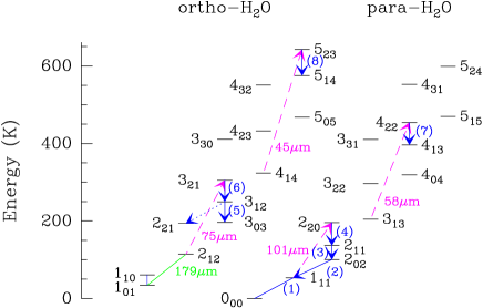
Figure 1: Energy level diagram of H₂O, showing the relevant H₂O lines at submillimeter wavelengths with blue arrows, and the far-IR H₂O pumping (absorption) lines with dashed-magenta arrows. The lines are numbered as listed in Table 1. The o-H₂O $3_{12}-2_{21}$ transition is not considered due to blending with CO (10-9) (G-A10), and the far-IR $2_{12}-1_{01}$ transition at $179.5$ $\mu$m discussed in the text is also indicated in green for completeness.

Table 2: Model parameters.

Parameter	Explored range	Best fit to
		HII+mild AGNa
$T_{\mathrm{dust}}$ (K)	$35-115$	$45-75$
$\tau_{100}$	$0.02-12$	$0.05-0.2$
$N_{\mathrm{H_{2}O}}/\Delta V$ (cm-2/(km s-1))	$3\times 10^{14}-10^{16}$	$(0.5-2)\times 10^{15}$
$\Delta V^{\mathrm{c}}$ (km s-1)	$100$	b
$n_{\mathrm{H_{2}}}$ (cm-3)	$2\times 10^{4}-3\times 10^{5}$	$\lesssim 3\times 10^{5}$
$T_{\mathrm{gas}}$ (K)	$100-200$	b

• Best fit values for HII+mild AGN sources (optically classified star-formation dominated galaxies with possible mild AGN contribution, see Y13 and Sect. 5) for which lines $2-6$ are detected, but lines $7-8$ are undetected.

• Parameter not well constrained.

• FWHM velocity dispersion of the dominant H₂O emitting structures, in our models equal to $1.67V_{\mathrm{turb}}$.

3 Description of the models

The basic models for H₂O were described in G-A10 (see also references therein). Summarizing, we assume a simple spherically symmetric source with uniform physical properties ($T_{\mathrm{dust}}$, $T_{\mathrm{gas}}$, gas and dust densities, H₂O abundance), where gas and dust are assumed to be mixed. We only consider the far-IR radiation field generated within the modeled source, ignoring the effect of external fields. The source is divided into a set of spherical shells where the statistical equilibrium level populations are calculated. The models are non-local, including line and continuum opacity effects. We assume an H₂O ortho-to-para ratio of 3. Line broadening is simulated by including a microturbulent velocity ($V_{\mathrm{turb}}$), for which the FWHM velocity dispersion is $\Delta V=1.67V_{\mathrm{turb}}$. No systemic motions are included.

3.1 Mass absorption coefficient of dust

The black curve in Fig. 2 shows the dust mass opacity coefficient used in the current and our past models (González-Alfonso et al., 2008, 2010, 2012, 2013, 2014). Our values at 125 and 850 $\mu$m are $\kappa_{125}=30$ cm² g^-1 and $\kappa_{850}=0.7$ cm² g^-1, in good agreement with those derived by Dunne et al. (2003). Adopting a gas-to-dust ratio of $X=100$ by mass, and using $\kappa_{100}=44.5$ cm² g^-1, the column density of H nuclei is

$$N_{\mathrm{H}}=\frac{X\,\tau_{100}}{m_{\mathrm{H}}\,\kappa_{100}}=1.3\times 10^{24}\,\tau_{100}\,\mathrm{cm^{-2}},$$ (1)

where $\tau_{100}$ is the continuum optical depth at 100 $\mu$m.

For this adopted dust composition, the fit across the far-IR to submm (blue line in Fig. 2) indicates an emissivity index of $\beta=1.85$, slightly steeper than the $\beta=1.5-1.6$ values favored by Kóvacs et al. (2010) and Casey (2012). The H₂O excitation is sensitive to the dust emission over a range of wavelengths (from $45$ to $270$ $\mu$m), but we find that our results on $L_{\mathrm{H_{2}O}}/L_{\mathrm{IR}}$ are insensitive to $\beta$ for $\beta$ values above $1.5$ (Sect. 4.3.3).

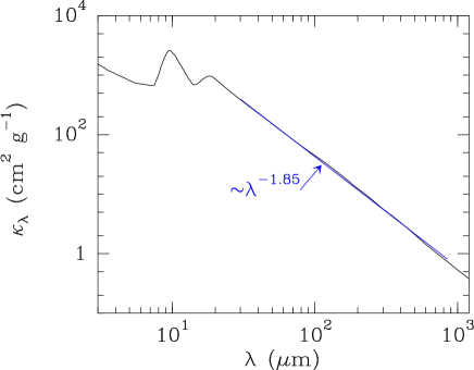
Figure 2: Adopted mass absorption coefficient of dust as a function of wavelength. The dust emission is simulated by using a mixture of silicate and amorphous carbon grains with optical constants from Draine (1985) and Preibisch et al. (1993). As shown by the fitted blue line, the emissivity index from the far-IR to millimeter wavelengths is $\beta=1.85$.

3.2 Model parameters

As listed in Table 2, the model parameters we have chosen to characterize the physical conditions in the emitting regions are $T_{\mathrm{dust}}$, the continuum optical depth at 100 $\mu$m along a radial path ($\tau_{100}$), the corresponding H₂O column density per unit of velocity interval ($N_{\mathrm{H_{2}O}}/\Delta V$), the velocity dispersion $\Delta V$, $T_{\mathrm{gas}}$, and the H₂ density ($n_{\mathrm{H_{2}}}$). Fiducial numbers for some of these parameters are $\tau_{100}=0.1$, $\Delta V=100$ km s^-1, $T_{\mathrm{gas}}=150$ K, and $n_{\mathrm{H_{2}}}=3\times 10^{5}$ cm^-3. Collisional rates with H₂ were taken from Dubernet et al. (2009) and Daniel et al. (2011). Our relevant results are the line-flux ratios ($F_{i}/F_{j}$) and the luminosity ratios $L_{\mathrm{H_{2}O}}/L_{\mathrm{IR}}$. We also explore models where collisions are ignored, appropriate for low-density regions ($n_{\mathrm{H_{2}}}\lesssim 10^{4}$ cm^-3), for which $F_{i}/F_{j}$ only depend on $T_{\mathrm{dust}}$, $\tau_{100}$, and $N_{\mathrm{H_{2}O}}/\Delta V$, while $L_{\mathrm{H_{2}O}}/L_{\mathrm{IR}}$ depends in addition on $\Delta V$.

Depending on the values of the above parameters, our models can be interpreted in terms of a single source or are better applied to each of an ensemble of clouds within a clumpy distribution. The radius of the modeled source is

$$R=N_{\mathrm{H}}/n_{\mathrm{H}}=0.21\times\left(\frac{\tau_{100}}{0.1}\right)\times\left(\frac{10^{5}\,\mathrm{cm^{-3}}}{n_{\mathrm{H_{2}}}}\right)\,\mathrm{pc},$$ (2)

where Eq. (1) has been applied. The corresponding IR luminosity can be written as $L_{\mathrm{IR}}=4\pi R^{2}\sigma T_{\mathrm{dust}}^{4}\,\gamma$, where $\gamma(T_{\mathrm{dust}},\tau_{100})\leq 1$ accounts for the departure from a blackbody emission due to finite optical depths, ranging from $\gamma=0.2$ for $T_{\mathrm{dust}}=50$ K and $\tau_{100}=0.1$ to $\gamma=0.9$ for $T_{\mathrm{dust}}=95$ K and $\tau_{100}=1$. In physical units,

$$L_{\mathrm{IR}}=1.4\times 10^{5}\times\left(\frac{\tau_{100}}{0.1}\right)^{2}\times\left(\frac{10^{5}\,\mathrm{cm^{-3}}}{n_{\mathrm{H_{2}}}}\right)^{2}\times\left(\frac{T_{\mathrm{dust}}}{55\,\mathrm{K}}\right)^{4}\times\left(\frac{\gamma}{0.2}\right)$$ (3)

in L_⊙, indicating that a model with $\tau_{100}\sim 0.1$ and moderate $T_{\mathrm{dust}}$ should be considered as one of an ensemble of clumps to account for the typically observed IR luminosities of $\gtrsim 10^{11}$ L_⊙ (Y13). For very warm ($T_{\mathrm{dust}}\sim 90$ K) and optically thick ($\tau_{100}\sim 1$) sources with low average densities ($n_{\mathrm{H_{2}}}=3\times 10^{3}$ cm^-3), Eq. (3) gives $L_{\mathrm{IR}}\sim 5\times 10^{11}$ L_⊙ and the model can be applied to a significant fraction of the circumnuclear region of galaxies where the clouds may have partially lost their individuality (Downes & Solomon, 1998).

The velocity dispersion $\Delta V$ in our models can be related to the velocity gradient used in escape probability methods as $dV/dr\sim\Delta V/(2R)$, and using Eq. (2)

$$dV/dr\sim 238\times\left(\frac{\Delta V}{100\,\mathrm{km\,s^{-1}}}\right)\times\left(\frac{0.1}{\tau_{100}}\right)\times\left(\frac{n_{\mathrm{H_{2}}}}{10^{5}\,\mathrm{cm^{-3}}}\right)\,\mathrm{km\,s^{-1}\,pc^{-1}.}$$ (4)

Defining $K_{\mathrm{vir}}$ as the ratio of the velocity gradient relative to that expected in gravitational virial equilibrium, $K_{\mathrm{vir}}=(dV/dr)/(dV/dr)_{\mathrm{vir}}$, and using $(dV/dr)_{\mathrm{vir}}\sim 10\times(n_{\mathrm{H_{2}}}/10^{5}\,\mathrm{cm^{-3}})^{1/2}$ $\mathrm{km\,s^{-1}\,pc^{-1}}$ (Bryant & Scoville, 1996; Goldsmith, 2001; Papadopoulos et al., 2007; Hailey-Dunsheath et al., 2012), we obtain

$$K_{\mathrm{vir}}\sim 23.8\times\left(\frac{\Delta V}{100\,\mathrm{km\,s^{-1}}}\right)\times\left(\frac{0.1}{\tau_{100}}\right)\times\left(\frac{n_{\mathrm{H_{2}}}}{10^{5}\,\mathrm{cm^{-3}}}\right)^{1/2}.$$ (5)

Values of $K_{\mathrm{vir}}$ significantly above 1 and up to $\sim 20$, indicating non-virialized phases, have been inferred in luminous IR galaxies from both low- and high-$J$ CO lines (e.g., Papadopoulos & Seaquist, 1999; Papadopoulos et al., 2007; Hailey-Dunsheath et al., 2012). For clarity, the velocity dispersion is rewritten in terms of $K_{\mathrm{vir}}$ as

$$\Delta V=42\times\left(\frac{K_{\mathrm{vir}}}{10}\right)\times\left(\frac{\tau_{100}}{0.1}\right)\times\left(\frac{10^{5}\,\mathrm{cm^{-3}}}{n_{\mathrm{H_{2}}}}\right)^{1/2}\,\mathrm{km\,s^{-1}},$$ (6)

which shows that, for compact and dense clumps ($\tau_{100}=0.1$, $n_{\mathrm{H_{2}}}=3\times 10^{5}$ cm^-3), $\Delta V\sim 25\times(K_{\mathrm{vir}}/10)$ km s^-1 and the typical observed linewidths ($\sim 300$ km s^-1) are caused by the galaxy rotation pattern and velocity dispersion of clumps. In contrast, for optically thick sources with low densities ($\tau_{100}=1$, $n_{\mathrm{H_{2}}}\lesssim 10^{4}$ cm^-3), $\Delta V\gtrsim 130$ km s^-1 is required for $K_{\mathrm{vir}}\gtrsim 1$.

Instead of calculating $\Delta V$ for each model according to eq. (6), which would involve a “universal” $K_{\mathrm{vir}}$ independent of the source characteristics, we have used $\Delta V=100$ km s^-1 for comparison purposes between models (in Sect. 4.3.5 we also consider models with constant $K_{\mathrm{vir}}$). Nevertheless, results can be easily rescaled to any other value of $\Delta V$ as follows. For given $T_{\mathrm{dust}}$ and $\tau_{100}$, the relative level populations, the line opacities, and thus the H₂O line-flux ratios ($F_{i}/F_{j}$) depend on $N_{\mathrm{H_{2}O}}/\Delta V$, while the luminosity ratios $L_{\mathrm{H_{2}O}}/L_{\mathrm{IR}}$ are proportional to $\Delta V$. Therefore, for any $\Delta V$, identical results for $F_{i}/F_{j}$ are obtained with the substitution

$$N_{\mathrm{H_{2}O}}\rightarrow N_{\mathrm{H_{2}O}}\times\left(\frac{\Delta V}{100\,\mathrm{km\,s^{-1}}}\right),$$ (7)

while $L_{\mathrm{H_{2}O}}/L_{\mathrm{IR}}$ should be scaled as

$$\frac{L_{\mathrm{H_{2}O}}}{L_{\mathrm{IR}}}\rightarrow\frac{L_{\mathrm{H_{2}O}}}{L_{\mathrm{IR}}}\times\left(\frac{\Delta V}{100\,\mathrm{km\,s^{-1}}}\right).$$ (8)

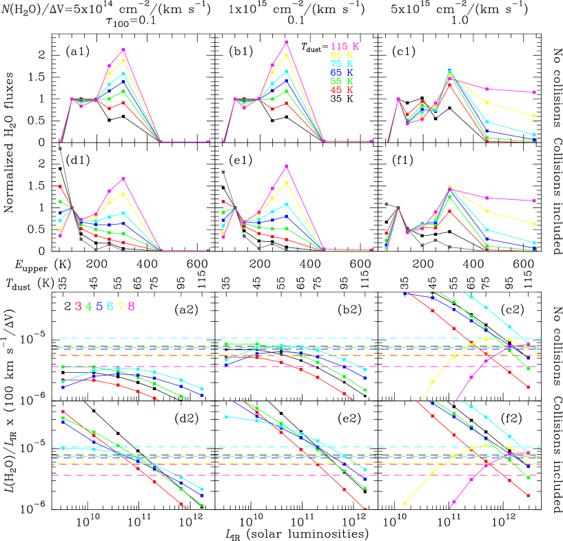
Figure 3: Relevant model results for the normalized H₂O SLED (a1-f1), and for the $L_{\mathrm{H_{2}O}}/L_{\mathrm{IR}}$ ratios (for $\Delta V=100$ km s^-1) as a function of $T_{\mathrm{dust}}$ and $L_{\mathrm{IR}}$ (assuming a source of $R_{\mathrm{eff}}=100$ pc, a2-f2). In panels a1-f1, model results for lines $1$ to $8$ (Table 1) are shown from left to right. Values for $N_{\mathrm{H_{2}O}}/\Delta V$ and $\tau_{100}$ are indicated at the top of the figure. The different colors in panels a1-f1 indicate different $T_{\mathrm{dust}}$, as labeled in b1, while they indicate different lines in panels a2-f2 (labeled in a2, see Table 1). Models with collisional excitation ignored (a-c), and with collisions included for $n_{\mathrm{H_{2}}}=3\times 10^{5}$ cm^-3 and $T_{\mathrm{gas}}=150$ K (d-f) are shown. The gray lines/symbols in panels d1-f1 show model results that ignore radiative pumping (i.e., only collisional excitation). Collisional excitation has the overall effect of enhancing the low-lying lines (1 and 2) relative to the others and of increasing the $L_{\mathrm{H_{2}O}}/L_{\mathrm{IR}}$ ratios of all lines (see text). The dashed lines in panels a2-f2 indicate the average $L_{\mathrm{H_{2}O}}/L_{\mathrm{IR}}$ ratios reported by Y13. When compared with observations, the modeled $L_{\mathrm{IR}}$ values should be considered a fraction of the observed IR luminosities, because single temperature dust models are unable to reproduce the observed SEDs (Sect. 4.3.1); the H₂O submm emission traces warm regions of luminous IR galaxies (see text).

Both the line-flux ratios ($F_{i}/F_{j}$) and the luminosity ratios $L_{\mathrm{H_{2}O}}/L_{\mathrm{IR}}$ are independent of the number of clumps ($N_{\mathrm{cl}}$) if the model parameters ($T_{\mathrm{dust}}$, $\tau_{100}$, $T_{\mathrm{gas}}$, $n_{\mathrm{H_{2}}}$, $N_{\mathrm{H_{2}O}}/\Delta V$, and $\Delta V$) remain the same for the cloud average. With the effective source radius defined as $R_{\mathrm{eff}}=N_{\mathrm{cl}}^{1/2}R$, both the line and continuum luminosities scale as $\propto R_{\mathrm{eff}}^{2}$. Therefore, if the effective source size is changed and all other parameters are kept constant, a linear correlation between each $L_{\mathrm{H_{2}O}}$ and $L_{\mathrm{IR}}$ is naturally generated, regardless of the excitation mechanism of H₂O. (For reference, however, all absolute luminosities below are given for $R_{\mathrm{eff}}=100$ pc.) The question, then, is what range of dust and gas parameters characterizes the sources for which the observed nearly linear correlations in lines $2-6$ (O13, Y13) are observed. The detection rates of lines $1$, $7$, and $8$ are relatively low, but the same trend is observed in the few sources where they are detected (Y13).

In the following sections, the general results of our models are presented, while specific fits to two extreme sources, Arp 220 and NGC 1068, are discussed in Appendix A.

4 Model results

4.1 General results

In Fig. 3, model results are shown in which $T_{\mathrm{dust}}$ is varied from 35 to 115 K, $N_{\mathrm{H_{2}O}}/\Delta V$ from $5\times 10^{14}$ to $5\times 10^{15}$ $\mathrm{cm^{-2}/(km\,s^{-1})}$, $\tau_{100}$ from $0.1$ to $1.0$, and where collisional excitation with $n_{\mathrm{H_{2}}}=3\times 10^{5}$ cm^-3 and $T_{\mathrm{gas}}=150$ K is excluded (a-c) or included (d-f). Panels a1-f1 (top) show the expected SLED normalized to line 2, and panels a2-f2 (bottom) plot the corresponding $L_{\mathrm{H_{2}O}}/L_{\mathrm{IR}}\times(100\,\mathrm{km\,s^{-1}}/\Delta V)$ ratios as a function of $T_{\mathrm{dust}}$ and $L_{\mathrm{IR}}$ (for $R_{\mathrm{eff}}=100$ pc; all points would move horizontally for different $R_{\mathrm{eff}}$). The effect of collisional excitation is also illustrated in Fig. 4, where the H₂O submm fluxes of lines $2-6$ relative to those obtained ignoring collisional excitation are plotted as a function of $n_{\mathrm{H_{2}}}$ for $T_{\mathrm{gas}}=150$ K.

The first conclusion that we infer from Fig. 3a1-f1 is that the relative fluxes of lines $5-6$ generally increase with increasing $T_{\mathrm{dust}}$. These lines are pumped through the H₂O transition at $\lambda\sim 75$ $\mu$m (Fig. 1), thus requiring warmer dust than lines $2-4$, which are pumped through absorption of 100 $\mu$m photons. The SLEDs obtained with $T_{\mathrm{dust}}<45$ K yield $F_{4}$ significantly above $F_{6}$, and are thus unlike those observed in most (U)LIRGs (Y13). The two peaks in the H₂O SLED (in lines 2 and 6) generally found in (U)LIRGs (Y13) indicate that the submm H₂O emission essentially samples regions with $T_{\mathrm{dust}}\gtrsim 45$ K. Significant collisional excitation enhances line 4 relative to line 6 (Fig. 3d1-f1), thus aggravating the discrepancy between the $T_{\mathrm{dust}}<45$ K models and the observations.

Lines $7-8$ provide stringent constraints on $T_{\mathrm{dust}}$, $\tau_{100}$, and $N_{\mathrm{H_{2}O}}/\Delta V$. Since line 6 is still easily excited even with moderately warm $T_{\mathrm{dust}}\sim 55$ K, the 8/6 and 7/6 ratios are good indicators of whether very warm dust ($>80$ K) is exciting H₂O. Sources where lines $7-8$ are detected (e.g., Mrk 231, Arp 220, and APM 08279) can be considered “very warm” on these grounds, with $N_{\mathrm{H_{2}O}}/\Delta V\gtrsim 3\times 10^{15}$ $\mathrm{cm^{-2}/(km\,s^{-1})}$. Sources where lines $7-8$ are not detected to a significant level, but where the SLED still shows a second peak in line 6, are considered “warm”, i.e. with $T_{\mathrm{dust}}$ varying between $\sim 45$ and 80 K, and $N_{\mathrm{H_{2}O}}/\Delta V\sim(5-20)\times 10^{14}$ $\mathrm{cm^{-2}/(km\,s^{-1})}$.

Sources in which lines $2-6$ are not detected to a significant level, that do not show a second peak in line 6, or for which the H₂O luminosities are well below the observed $L_{\mathrm{H_{2}O}}-L_{\mathrm{IR}}$ correlation are considered “cold”. These sources are characterized by very optically thin and extended continuum emission, and/or with low $N_{\mathrm{H_{2}O}}$ (these properties likely go together). Such sources include starbursts like M82 (Y13), where the continuum is generated in PDRs and are physically very different from the properties of “very warm” sources like Mrk 231 (G-A10).

In the models that neglect collisional excitation (a1-c1), line 1 is predicted to be in absorption, transitioning to emission in warm/dense regions where it is collisionally excited (d1-f1), as previously argued. Its strength will also depend on the continuum opacity, which should be low enough to allow the line to emit above the continuum. Direct collisional excitation from the ground state in regions with warm gas but low $\tau_{100}$ efficiently populates level $2_{02}$, so that the 2/3, 2/4, 2/5, and 2/6 ratios strongly increase with increasing $n_{\mathrm{H_{2}}}$ (Fig. 4a). As advanced in Sect. 2, collisional excitation also boosts all other submm lines for moderate $T_{\mathrm{dust}}$ owing to efficient pumping of the base levels $2_{12}$ and $1_{11}$; radiative trapping of photons emitted in the ground-state transitions increases the chance of absorption of continuum photons in the $101$ and $75$ $\mu$m transitions. Nevertheless, collisional excitation is negligible for high $\tau_{100}$ and high $T_{\mathrm{dust}}$ (Fig. 4b).

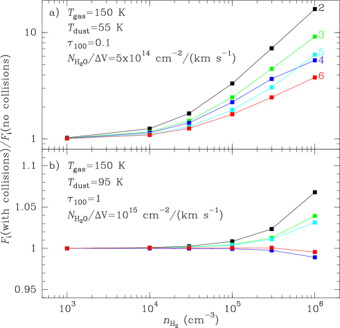
Figure 4: Effect of collisional excitation on the H₂O fluxes of the submm lines $2-6$ as a function of $n_{\mathrm{H_{2}}}$. The ordinates show the calculated line fluxes relative to the model that ignores collisional excitation. $T_{\mathrm{gas}}=150$ K is adopted in all models. a) In the case of moderate $T_{\mathrm{dust}}$ and low $\tau_{100}$, collisional excitation has a strong impact on the H₂O fluxes at $n_{\mathrm{H_{2}}}$ of $\mathrm{a\,few\times 10^{4}}$ cm^-3, especially on line 2. b) Collisional excitation is negligible for high $\tau_{100}$ and very warm $T_{\mathrm{dust}}$ (note the difference in ordinate scales in a) and b)).

4.2 Predicted line ratios

In sources where lines 7 and 8 are not detected, the 6/4 flux ratio is the most direct indication of the hardness of the far-IR radiation field seen by the H₂O gas responsible for the observed emission. Since line 4 is pumped through absorption of 101 $\mu$m photons and line 6 by 75 $\mu$m photons (Fig. 1), one may expect a correlation between the 6/4 ratio and the 75-to-100 $\mu$m far-IR color, $f_{75}/f_{100}$. As shown in Fig. 5a, our models indeed show a steep increase in the 6/4 ratio with $T_{\mathrm{dust}}$ for fixed $\tau_{100}$ and $N_{\mathrm{H_{2}O}}$. The averaged observed 6/4 ratio of $\approx 1.45-1.7$ in strong-AGN and HII+mild-AGN sources (Y13) indicates, assuming an optically thin continuum (Fig. 5a), $T_{\mathrm{dust}}\approx 55-75$ K and $f_{75}/f_{100}=1.5-1.8$. For the case of high $\tau_{100}$ and $N_{\mathrm{H_{2}O}}/\Delta V$, the averaged 6/4 ratio is consistent with lower $T_{\mathrm{dust}}$ and $f_{75}/f_{100}=1-1.2$. In general, the 6/4 ratio indicates $T_{\mathrm{dust}}\approx 45-80$ K. Similarly, the 6/2 ratio is also sensitive to $T_{\mathrm{dust}}$, as shown in Fig. 5b. The observed averaged 6/2 ratio of $\approx 1-1.2$ is compatible with $T_{\mathrm{dust}}$ somewhat lower than estimated from the 6/4 ratio. This is attributable to the effects of collisional excitation of the $2_{02}$ level (thus enhancing line 2 over line 6, see Fig. 4a and magenta symbols in Fig. 5b), or to the contribution to line 2 by an extended, low $T_{\mathrm{dust}}$ component.

There is, however, no observed correlation between the 6/4 ratio and $f_{60}/f_{100}$ (Y13), which should still show a correlation (though maybe less pronounced) than the expected correlation with $f_{75}/f_{100}$. As we argue in Sect. 4.3, this lack of correlation suggests that the observed far-IR $f_{60}/f_{100}$ colors, and in particular the observed $f_{100}$ fluxes, are not dominated by the warm component responsible for the H₂O emission. Indeed, current models for the continuum emission in (U)LIRGs indicate that the flux density at 100 $\mu$m is dominated by relatively cold dust components ($T_{\mathrm{dust}}\sim 30$ K) (e.g. Dunne et al., 2003; Kóvacs et al., 2010; Casey, 2012). The observed H₂O emission thus arises in warm regions whose continuum is hidden within the observed far-IR emission, but may dominate the observed SED at $\lambda\lesssim 50$ $\mu$m (e.g., Casey, 2012, see also Sect. 4.3.1).

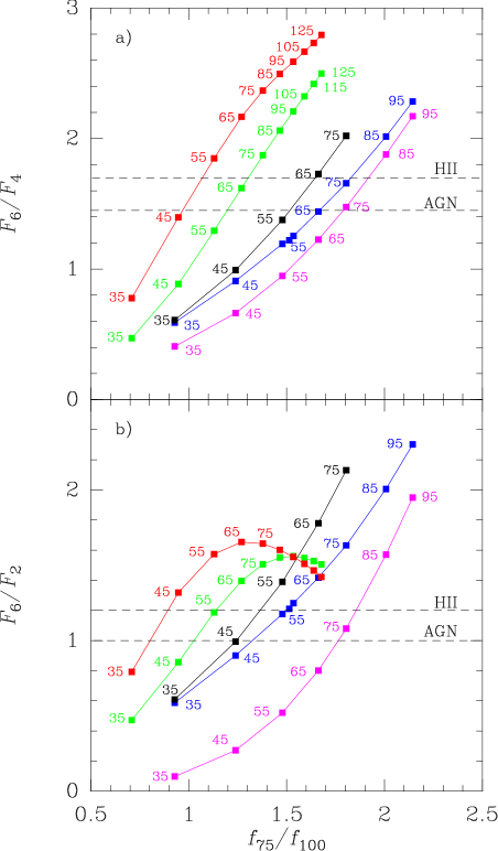
Figure 5: a) $F_{6}/F_{4}$ (oH₂O $3_{21}-3_{12}$-to-pH₂O $2_{20}-2_{11}$) and b) $F_{6}/F_{2}$ (oH₂O $3_{21}-3_{12}$-to-pH₂O $2_{02}-1_{11}$) line flux ratios as a function of the 75-to-100 $\mu$m far-IR color. Blue symbols: $N_{\mathrm{H_{2}O}}/\Delta V=10^{15}$ $\mathrm{cm^{-2}/(km\,s^{-1})}$ and $\tau_{100}\leq 0.1$; black: $N_{\mathrm{H_{2}O}}/\Delta V=5\times 10^{15}$ $\mathrm{cm^{-2}/(km\,s^{-1})}$ and $\tau_{100}\leq 0.1$; red: $N_{\mathrm{H_{2}O}}/\Delta V=5\times 10^{15}$ $\mathrm{cm^{-2}/(km\,s^{-1})}$ and $\tau_{100}=1.0$; green: $N_{\mathrm{H_{2}O}}/\Delta V=10^{15}$ $\mathrm{cm^{-2}/(km\,s^{-1})}$ and $\tau_{100}=1.0$; magenta: same as blue symbols but with collisional excitation included with $T_{\mathrm{gas}}=150$ K and $n_{\mathrm{H_{2}}}=3\times 10^{5}$ cm^-3. The small numbers close to the symbols indicate the value of $T_{\mathrm{dust}}$. The observed averaged ratios for strong-AGN and HII+mild-AGN sources (Y13) are indicated with dashed horizontal lines, and indicate that the regions probed by the H₂O submm emission are characterized by warm dust ($T_{\mathrm{dust}}\gtrsim 45$ K).

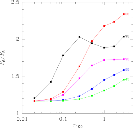
Figure 6: $F_{6}/F_{5}$ (oH₂O $3_{21}-3_{12}$-to-$3_{12}-3_{03}$) line flux ratio as a function of $\tau_{100}$. The small numbers on the right side of the curves indicate the values of $T_{\mathrm{dust}}$ for each curve. The H₂O column density per unit of velocity interval is $N_{\mathrm{H_{2}O}}/\Delta V=10^{15}$ $\mathrm{cm^{-2}/(km\,s^{-1})}$ (green, blue, and magenta curves) and $N_{\mathrm{H_{2}O}}/\Delta V=5\times 10^{15}$ $\mathrm{cm^{-2}/(km\,s^{-1})}$ (red and black curves).

The H₂O lines 5 and 6 are both pumped through the 75 $\mu$m transition. Assuming that the lines are optically thin, statistical equilibrium of the level populations implies that every de-excitation in line 6 will be followed by a de-excitation in either line 5 or in the $3_{12}-2_{21}$ transition (dotted arrow in Fig. 1), with relative probablities determined by the A-Einstein coefficients. In these optically thin conditions, we expect a 6/5 line flux ratio of $F_{6}/F_{5}=1.16$ (Fig. 6). This is a lower limit, because in case of high $N_{\mathrm{H_{2}O}}/\Delta V$ and/or high $T_{\mathrm{dust}}$ and $\tau_{100}$, absorption of line 5 emitted photons that can eventually be reemited through the $3_{12}-2_{21}$ transition, or absorption of continuum photons in the H₂O $4_{23}-3_{12}$ transition, will decrease the strength of line 5 relative to line 6.

Although with significant dispersion, overall data for HII+mild AGN sources indicate $F_{6}/F_{5}\sim 1.2$ (Y13), consistent with the optically thin limit; examples of this galaxy population are NGC 1068 and NGC 6240 (Spinoglio et al., 2012; Meijerink et al., 2013). There are, however, sources like Arp 220 and Mrk 231 with $F_{6}/F_{5}\approx 1.6$, favoring warm dust ($>55$ K) and substantial columns of H₂O and dust. This indicates that sources in both the optically thin and optically thick regimes are H₂O emitters.

In optically thin conditions and with moderate $T_{\mathrm{dust}}$, lines $2-4$, together with the pumping $2_{20}-1_{11}$ 101 $\mu$m transition, form a closed loop (Fig. 1) where statistical equilibrium of the level populations implies equal fluxes for the three submm lines (Fig. 3a1-c1). The rise in $T_{\mathrm{dust}}$ and $\tau_{100}$, however, increases the chance of line absorption in the strong $3_{22}-2_{11}$ transition at 90 $\mu$m, thus decreasing the flux of line 3 relative to both line 2 and 4. Consequently, the $F_{2}/F_{3}$ ratio is expected to increase from $\approx 1$ (for low $\tau_{100}$) to $\approx 2$ (for $\tau_{100}\sim 1$ and $N_{\mathrm{H_{2}O}}/\Delta V\gtrsim 10^{17}$ $\mathrm{cm^{-2}/(km\,s^{-1})}$), consistent with the relatively high values found in the warm Mrk 231 and APM 08279 (Y13). If collisional excitation is important (Fig. 3d-f), $F_{2}/F_{3}$ is also expected to increase because collisions mainly boost the lower lying line 2 (Fig. 4a).

One interesting caveat is, however, the behavior of the 4/3 ratio, because increasing $T_{\mathrm{dust}}$ and/or $N_{\mathrm{H_{2}O}}$ is predicted to increase $F_{2}/F_{3}$ but maintains $F_{4}/F_{3}>1$ (Fig. 3a1-c1). In Mrk 231, the high $F_{2}/F_{3}$ ratio and mostly the detection of lines $7-8$ indicate very warm dust (G-A10), but the relatively low $F_{4}/F_{3}\lesssim 1$ observed in the source does not match this simple scheme. The problem is exacerbated with the 6/2 ratio, which is also expected to increase with increasing $T_{\mathrm{dust}}$ and $\tau_{100}$ to $\approx 1.5$ (Fig. 5), but Mrk 231 shows $F_{6}/F_{2}\approx 1$. Nevertheless, the problem can be solved if source structure is invoked. A composite model where a very warm component accounts for the high-lying lines and a colder (dust) component enhances lines $2-4$ (with probable contribution from collisionally excited gas, as suggested by the high $F_{2}/F_{3}$ ratio), can give a good fit to the SLED (G-A10), although the characteristics of the “cold” component (density, extension, $T_{\mathrm{dust}}$) are relatively uncertain. A relatively low flux in line 4 can also be produced by absorption of continuum photons emanating from a very optically thick component, as in Arp 220 (see App. A).

4.3 The $L_{\mathrm{H_{2}O}}-L_{\mathrm{IR}}$ correlations

4.3.1 H₂O and the observed SED

It has long been recognized that single-temperature graybody fits to galaxy SEDs at far-IR wavelengths often underpredict the observed emission at $\lambda<50$ $\mu$m. Therefore, multicomponent fitting, based on, for example, a two-temperature approach, a power-law mass-temperature distribution, a power-law mass-intensity distribution, or a single cold dust temperature graybody with a mid-IR power law (Dunne et al., 2003; Kóvacs et al., 2010; Dale & Helou, 2002; Casey, 2012), is required to match the full SED from the mid-IR to millimeter wavelengths. Our single-temperature model results on the H₂O SLED favors $T_{\mathrm{dust}}\gtrsim 45$ K (Sect. 4.2), significantly warmer than the cold dust temperatures ($<40$ K) that account for most of the observed far-IR emission in luminous IR galaxies, indicating that the H₂O submm emission primarily probes the warm region(s) of galaxies where the mid-IR ($20-50$ $\mu$m) emission is generated (see footnote 5).

Relative to the total IR emission of a galaxy, $L_{\mathrm{IR}}^{T}$, the contribution to the luminosity by a given $T_{\mathrm{dust}}$ component $i$ is $f_{i}=L_{\mathrm{IR}}^{i}/L_{\mathrm{IR}}^{T}$, and the observed H₂O-to-IR luminosity ratio is

$$\frac{L_{\mathrm{H_{2}O}}}{L_{\mathrm{IR}}^{T}}=\sum_{i}f_{i}\left(\frac{L_{\mathrm{H_{2}O}}}{L_{\mathrm{IR}}}\right)_{i}=f_{\mathrm{warm}}\left(\frac{L_{\mathrm{H_{2}O}}}{L_{\mathrm{IR}}}\right)_{\mathrm{warm}}+f_{\mathrm{cold}}\left(\frac{L_{\mathrm{H_{2}O}}}{L_{\mathrm{IR}}}\right)_{\mathrm{cold}}$$ (9)

where $(L_{\mathrm{H_{2}O}}/L_{\mathrm{IR}})_{i}$ are the values plotted in Fig. 3a2-f2 (for $\Delta V=100$ km s^-1), and the problem is grossly simplified by considering only two “warm” and “cold” components. From the comparison of the observed average SLED (Y13) with our models, we infer that the contribution by the cold component to $L_{\mathrm{H_{2}O}}/L_{\mathrm{IR}}^{T}$ is small, even though $f_{\mathrm{cold}}$ may be high. Since our modeled $L_{\mathrm{IR}}$ emission from the warm component is thus only a fraction, $f_{\mathrm{warm}}$, of the total IR budget, the modeled $L_{\mathrm{H_{2}O}}/L_{\mathrm{IR}}$ ratios in Fig. 3a2-f2 should be considered upper limits. The value of $f_{\mathrm{warm}}$ can only be estimated by fitting the individual SEDs.

4.3.2 H₂O emission and monochromatic luminosities

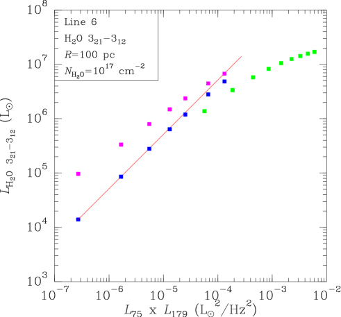
Figure 7: Model results showing the luminosity of the H₂O line 6 ($3_{21}-3_{12}$) as a function of the product of the monochromatic luminosities at 75 and 179 $\mu$m. Luminosities are calculated for a source with $R_{\mathrm{eff}}=100$ pc, $N_{\mathrm{H_{2}O}}/\Delta V=10^{15}$ $\mathrm{cm^{-2}/(km\,s^{-1})}$, and $\Delta V=100$ km s^-1. Blue squares indicate models with $\tau_{100}=0.1$, resulting in optically thin or moderately thick H₂O emission, without collisional excitation. Magenta squares show results for the same models but with collisional excitation included with $T_{\mathrm{gas}}=150$ K and $n_{\mathrm{H_{2}}}=3\times 10^{5}$ cm^-3. Green symbols indicate models with $\tau_{100}=1.0$, resulting in optically thick H₂O emission. For optically thin H₂O emission and without collisional excitation, the models indicate a linear correlation between $L_{\mathrm{H_{2}O}}$ and $L_{75}\times L_{179}$ (red line).

The H₂O submm emission of lines $2-6$ essentially involves two excitation processes, that of the base level ($2_{12}$ for ortho and $1_{11}$ for para-H₂O) and absorption in the transitions at 75 $\mu$m (ortho) or 101 $\mu$m (para, Fig. 1). If collisional excitation is unimportant, the excitation of the base levels is also produced by absorption of dust-emitted photons in the corresponding transitions, i.e., in the $2_{12}-1_{01}$ line at 179 $\mu$m (ortho) or $1_{11}-0_{00}$ at 269 $\mu$m (para). In optically thin conditions and for fixed $N_{\mathrm{H_{2}O}}$ and $\Delta V$, our models then show a linear correlation between the H₂O luminosities $L_{\mathrm{H_{2}O}}$ and the product of the continuum monochromatic luminosities responsible for the excitation, $L_{179}\times L_{75}$ (ortho) or $L_{269}\times L_{101}$ (para). This linear correlation is illustrated in Fig. 7 for line 6. The linear correlation, however, breaks down when the line becomes optically thick or when collisional excitation becomes important (in which case, $L_{\mathrm{H_{2}O}}$ is independent of $L_{179(269)}$).

4.3.3 The $L_{\mathrm{H_{2}O}}/L_{\mathrm{IR}}$ ratios and $T_{\mathrm{dust}}$

The above considerations are relevant for our understanding of the behavior of the modeled $L_{\mathrm{H_{2}O}}/L_{\mathrm{IR}}$ values with variations in $T_{\mathrm{dust}}$. In the optically thin case and with collisional excitation ignored, the double dependence of $L_{\mathrm{H_{2}O}}$ on two monochromatic luminosities implies that $L_{\mathrm{H_{2}O}}$ is (nearly) proportional to $L_{\mathrm{IR}}$. Our predicted SEDs indicate that, for small variations in $T_{\mathrm{dust}}$ around $55$ K, $L_{269}\propto L_{\mathrm{IR}}^{2/7}$ and $L_{101}\propto L_{\mathrm{IR}}^{1/2}$. Therefore, for the para-H₂O lines $2-4$, $L_{2-4}\propto L_{\mathrm{IR}}^{0.8}$ in optically thin conditions, slightly slower than linear. For the ortho lines, $L_{179}\propto L_{\mathrm{IR}}^{1/3}$ and $L_{75}\propto L_{\mathrm{IR}}^{2/3}$, so that $L_{5-6}\propto L_{\mathrm{IR}}$. This explains why, in Fig. 3(a2-b2), the $L_{\mathrm{2-4}}/L_{\mathrm{IR}}$ ratios show a slight decrease with increasing $T_{\mathrm{dust}}$ above 55 K, while $L_{\mathrm{5-6}}/L_{\mathrm{IR}}$ versus $T_{\mathrm{dust}}$ attain a maximum at $T_{\mathrm{dust}}\approx 55$ K in optically thin models that omit collisional excitation. These results are robust against variations in the spectral index of dust down to $\beta=1.5$ (Sect. 3.1).

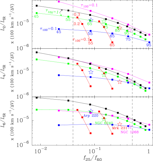
Figure 8: Modeled $L_{\mathrm{H_{2}O}}/L_{\mathrm{IR}}\times(100\,\mathrm{km\,s^{-1}}/\Delta V)$ for lines 2 (upper), 4 (middle), and 6 (lower) as a function of the $f_{25}/f_{60}$ color. The dashed vertical lines indicate the lower and upper limits for $f_{25}/f_{60}$ measured by Y13. In the upper panel, the small numbers below the squares indicate the value of $T_{\mathrm{dust}}$, and $\tau_{100}$ is also indicated. Blue squares: $N_{\mathrm{H_{2}O}}/\Delta V=10^{15}$ $\mathrm{cm^{-2}/(km\,s^{-1})}$ and $\tau_{100}=0.1$; magenta: same as blue symbols but with collisional excitation included with $T_{\mathrm{gas}}=150$ K and $n_{\mathrm{H_{2}}}=3\times 10^{5}$ cm^-3; green: $N_{\mathrm{H_{2}O}}/\Delta V=10^{15}$ $\mathrm{cm^{-2}/(km\,s^{-1})}$ and $\tau_{100}=1.0$; black: same as green but with $N_{\mathrm{H_{2}O}}/\Delta V=5\times 10^{15}$ $\mathrm{cm^{-2}/(km\,s^{-1})}$. Red squares show results for fixed $T_{\mathrm{dust}}=55$ and $65$ K with $N_{\mathrm{H_{2}O}}/(\Delta V\tau_{100})=5\times 10^{15}$ $\mathrm{cm^{-2}/(km\,s^{-1})}$ and $\tau_{100}=0.1-0.3$. The starred symbols indicate the positions of Arp 220 (blue), NGC 6240 (green), Mrk 231 (red), and NGC 1068 (magenta), as reported by Rangwala et al. (2011), Meijerink et al. (2013), G-A10, and Y13, respectively. When compared with observations, the modeled $L_{\mathrm{IR}}$ values should be considered a fraction of the observed IR luminosities (Sect. 4.3.1). If $f_{60}$ is contaminated by cold dust, the points would move to the left.

In Fig. 8 we show the $L_{\mathrm{H_{2}O}}/L_{\mathrm{IR}}$ ratios (with $\Delta V=100$ km s^-1; $L_{\mathrm{H_{2}O}}/L_{\mathrm{IR}}\propto\Delta V$) for lines 2, 4, and 6 as a function of the $f_{25}/f_{60}$ color. The observed $f_{25}/f_{60}$ was used by Y13 to characterize the H₂O emission and is especially relevant given that the H₂O submm emission arises in warm regions in which the mid-IR continuum emission is not severely contaminated by cold dust. However, the continuum at $\lambda=60$ $\mu$m may still be contaminated to some extent, in which case the data points in Fig. 8 will move toward the left. We also recall that the $L_{\mathrm{H_{2}O}}/L_{\mathrm{IR}}$ values are upper limits.

The first conclusion inferred from Fig. 8 is that the range of $f_{25}/f_{60}$ colors measured by Y13 (between the dashed lines) matches $T_{\mathrm{dust}}$ in the ranges favored by the observed H₂O line flux ratios, that is, $50-75$ K and optically thin conditions ($\tau_{100}=0.1$) and also $T_{\mathrm{dust}}=60-95$ K and $\tau_{100}=1.0$. This indicates that the warm environments responsible for the H₂O emission are best traced in the continuum in this wavelength range, but also that the $f_{25}/f_{60}$ color alone involves degeneracy in the dominant $T_{\mathrm{dust}}$ and $\tau_{100}$ responsible for the mid-IR continuum emission. As shown in Sect. 4.2, the first set of conditions can explain the line ratios $2-6$ in warm sources (where lines $7-8$ are not detected to a significant level), while the second set is required to explain the H₂O emission in very warm sources (with detection of lines $7-8$).

Second, it is also relevant that the $L_{\mathrm{H_{2}O}}/L_{\mathrm{IR}}$ values differ by a factor $\lesssim 2$ between models with warm dust in the optically thin regime ($T_{\mathrm{dust}}=55$ K, $\tau_{100}=0.1$, $N_{\mathrm{H_{2}O}}/\Delta V=10^{15}$ $\mathrm{cm^{-2}/(km\,s^{-1})}$) and those with very warm dust in the optically thick regime with high H₂O columns ($T_{\mathrm{dust}}=95$ K, $\tau_{100}=1$, $N_{\mathrm{H_{2}O}}/\Delta V=5\times 10^{15}$ $\mathrm{cm^{-2}/(km\,s^{-1})}$), potentially explaining why sources with different physical conditions show similar $L_{\mathrm{H_{2}O}}/L_{\mathrm{IR}}$ ratios (Y13).

Third, in optically thin conditions ($\tau_{100}\sim 0.1$) and if collisional excitation is unimportant, the models with constant $N_{\mathrm{H_{2}O}}/\Delta V=10^{15}$ $\mathrm{cm^{-2}/(km\,s^{-1})}$ (blue symbols) predict a slow decrease in $L_{2-4}/L_{\mathrm{IR}}$ and a nearly constant $L_{5-6}/L_{\mathrm{IR}}$ with increasing $f_{25}/f_{60}$, as argued above. This behavior, however, fails to match the observed trends (Y13), as $L_{2-4}/L_{\mathrm{IR}}$ and $L_{6}/L_{\mathrm{IR}}$ decrease by factors of $\sim 2$ and $\sim 3$, respectively, when $f_{25}/f_{60}$ increases from $\lesssim 0.08$ to $\gtrsim 0.15$. When collisional excitation is included (magenta symbols), the $L_{2-4}/L_{\mathrm{IR}}$ ratios show a stronger dependence on $f_{25}/f_{60}$, but $L_{6}/L_{\mathrm{IR}}$ still changes only slightly with $f_{25}/f_{60}$.

Therefore, optically thin models with varying $T_{\mathrm{dust}}$ but constant $\tau_{100}$, $N_{\mathrm{H_{2}O}}/\Delta V$, and $\Delta V$ cannot account for the observed $L_{\mathrm{H_{2}O}}/L_{\mathrm{IR}}-f_{25}/f_{60}$ trend. This indicates that, in optically thin galaxies, parameters other than $T_{\mathrm{dust}}$ are systematically varied when $f_{25}/f_{60}$ is increased and that optically thick sources also contribute to the observed trend:
($i$) Galaxies in the optically thin regime (with $\tau_{100}<1$) are predicted to show a very steep dependence of $L_{\mathrm{H_{2}O}}/L_{\mathrm{IR}}$ on $\tau_{100}$ for constant $T_{\mathrm{dust}}$ and $N_{\mathrm{H_{2}O}}/(\Delta V\tau_{100})$ (that is, for constant H₂O abundance), with higher $\tau_{100}$ impling lower $f_{25}/f_{60}$. We illustrate this point in Fig. 8 with the red squares, corresponding to fix $T_{\mathrm{dust}}=55$ and $65$ K and $N_{\mathrm{H_{2}O}}/(\Delta V\tau_{100})=5\times 10^{15}$ $\mathrm{cm^{-2}/(km\,s^{-1})}$, with $\tau_{100}$ ranging from $0.1$ to $0.3$. Therefore, we expect that the observed increase in $f_{25}/f_{60}$ is not only due to an increase in $T_{\mathrm{dust}}$ from source to source, but also to variations in $\tau_{100}$ in the optically thin regime. Examples of galaxies in this regime are the AGNs NGC 6240 and NGC 1068 (see also App. A).
($ii$) In the optically thick regime ($\tau_{100}\gtrsim 1$), galaxies are also predicted to show a relatively steep variation in $L_{\mathrm{H_{2}O}}/L_{\mathrm{IR}}$ with $f_{25}/f_{60}$ due to increasing $T_{\mathrm{dust}}$ (black symbols in Fig. 8) because the H₂O lines saturate and their luminosities flatten with increasing monochromatic luminosities (Fig. 7). Extreme examples of this galaxy population are Arp 220 and Mrk 231. Line saturation also implies that the $L_{\mathrm{H_{2}O}}/L_{\mathrm{IR}}$ ratios are not much higher than in the optically thin case even if much higher $N_{\mathrm{H_{2}O}}/\Delta V=5\times 10^{15}$ $\mathrm{cm^{-2}/(km\,s^{-1})}$ are present, and the corresponding ratios are consistent with the observed values to within the uncertainties in $f_{\mathrm{warm}}$. The presence of even warmer dust ($>100$ K) with significant contribution to $L_{\mathrm{IR}}$ will additionally decrease $L_{\mathrm{H_{2}O}}/L_{\mathrm{IR}}$ (Y13).

In summary, the steep decrease in $L_{\mathrm{H_{2}O}}/L_{\mathrm{IR}}$ at $f_{25}/f_{60}\approx 0.1-0.15$ measured by Y13 is consistent with both types of galaxies (with optically thin and optically thick continuum) populating the diagram and suggests that the observed variations in $f_{25}/f_{60}$ are not only due to variations in $T_{\mathrm{dust}}$ but also to variations in $\tau_{100}$ in the optically thin regime. At the other extreme, the optically thick (saturated) and very warm galaxies are also expected to show a decrease in $L_{\mathrm{H_{2}O}}/L_{\mathrm{IR}}$ with increasing $T_{\mathrm{dust}}$ (and $f_{25}/f_{60}$), as anticipated by Y13. To distinguish between both regimes for a given galaxy, the line ratios (specifically $F_{6}/F_{5}$, Sect. 4.2) and mostly the detection of lines $7-8$ or the detection of high-lying H₂O absorption lines at far-IR wavelengths are required. The observations reported by Y13 indicate that these optically thick and warm components (diagnosed by the detection of lines $7-8$) are present in at least ten sources. At least in NGC 1068 the upper limits on lines $7-8$ are stringent (S12), allowing us to infer optically thin conditions.

4.3.4 Line saturation and a theoretical upper limit to $L_{\mathrm{H_{2}O}}/L_{\mathrm{IR}}$

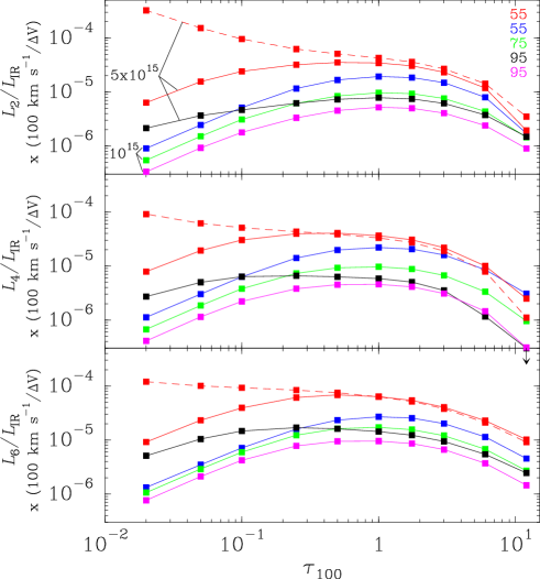
Figure 9: Modeled $L_{\mathrm{H_{2}O}}/L_{\mathrm{IR}}\times(100\,\mathrm{km\,s^{-1}}/\Delta V)$ values for lines 2 (upper), 4 (middle), and 6 (lower) as a function of $\tau_{100}$. Collisional excitation is ignored except for the red dashed lines, where $T_{\mathrm{gas}}=150$ K and $n_{\mathrm{H_{2}}}=3\times 10^{5}$ cm^-3 are adopted. The small numbers on the right side of the upper panel indicate the value of $T_{\mathrm{dust}}$ in K, and those on the left side indicate $N_{\mathrm{H_{2}O}}/\Delta V$ in $\mathrm{cm^{-2}/(km\,s^{-1})}$. When compared with observations, the modeled $L_{\mathrm{IR}}$ values should be considered a fraction of the observed IR luminosities (Sect. 4.3.1). For $\tau_{100}=12$ and $T_{\mathrm{dust}}=95$ K, line 4 is predicted to be in absorption. For fixed $T_{\mathrm{dust}}$ and $\tau_{100}\sim 1$, the $L_{\mathrm{H_{2}O}}/L_{\mathrm{IR}}$ ratios are similar for very different $N_{\mathrm{H_{2}O}}$, indicating line saturation.

Saturation of the H₂O submm lines in optically thick ($\tau_{100}\sim 1$) sources implies that there is an upper limit on $L_{\mathrm{H_{2}O}}/L_{\mathrm{IR}}\times(100\,\mathrm{km\,s^{-1}}/\Delta V)$ that, in the absence of significant collisional excitation, cannot be exceeded. In Fig. 9, the $L_{\mathrm{H_{2}O}}/L_{\mathrm{IR}}\times(100\,\mathrm{km\,s^{-1}}/\Delta V)$ ratios for lines 2, 4, and 6 are plotted as a function of $\tau_{100}$ for the most favored $T_{\mathrm{dust}}$ range of $55-95$ K and $N_{\mathrm{H_{2}O}}/\Delta V=(1-5)\times 10^{15}$ $\mathrm{cm^{-2}/(km\,s^{-1})}$. In optically thin conditions ($\tau_{100}\lesssim 0.1$ for $N_{\mathrm{H_{2}O}}/\Delta V=10^{15}$ $\mathrm{cm^{-2}/(km\,s^{-1})}$) and without collisions, $L_{\mathrm{H_{2}O}}/L_{\mathrm{IR}}$ scales linearly (for fixed $\Delta V$) with $\tau_{100}$ because $L_{179(269)}\times L_{75(101)}\propto\tau_{100}^{2}$ while $L_{\mathrm{IR}}\propto\tau_{100}$. The curves flatten as the H₂O lines saturate and show a maximum at $\tau_{100}\approx 0.5-1$. Values of $\tau_{100}$ significantly higher than unity are predicted to decrease $L_{\mathrm{H_{2}O}}/L_{\mathrm{IR}}$. In very optically thick components of very warm sources, the submm lines are predicted to be observed in weak emission or even in absorption, especially in line 4. Arp 220 is a case in point (Sakamoto et al., 2008), in which the H₂O submm emission is expected to arise from a region that surrounds the optically thick nuclei (see App. A). For $\Delta V=100$ km s^-1, the maximum attainable values of $L_{\mathrm{H_{2}O}}/L_{\mathrm{IR}}$ (red curves) are $3.5\times 10^{-5}$, $4\times 10^{-5}$, and $7\times 10^{-5}$ for lines 2, 4, and 6, respectively, comfortably higher than the values observed in any source by Y13. Recently, a value of $L_{2}/L_{\mathrm{IR}}=(4.3\pm 1.6)\times 10^{-5}$ has been measured in the submillimeter galaxy SPT 0538-50, a gravitationally lensed dusty star-forming galaxy at $z\approx 2.8$ (Bothwell et al., 2013). Although the authors do not exclude differential lensing effects, which could affect the line-to-luminosity ratios, this value is still consistent with our upper limit, suggesting strong saturation in this source. In HFLS3 at $z=6.34$, Riechers et al. (2013) have measured $F_{6}/F_{2}=2.2\pm 0.5$ and $F_{6}/F_{5}=2.6\pm 0.8$; within the uncertainties, these values are consistent with warm or very warm $T_{\mathrm{dust}}\gtrsim 65$ K and high $N_{\mathrm{H_{2}O}}$ (Figs. 5-6). The H₂O lines are most likely saturated in HFLS3 as is also indicated by the $L_{6}/L_{\mathrm{IR}}=(7.7\pm 1.3)\times 10^{-5}$ ratio, which is still consistent with the strong saturation limit for warm $T_{\mathrm{dust}}$ given the very broad linewidth of the H₂O line ($\sim 940$ km s^-1; see Sect 3.2). O13 reported $L_{2}/L_{\mathrm{IR}}=(0.5-2)\times 10^{-5}$ in high-$z$ ultra-luminous infrared galaxies, also consistent with the upper limit in Fig. 9 even for $T_{\mathrm{dust}}\sim 75$ K when taking the broad line widths of the H₂O lines into account. Line saturation and a relatively small contribution from cold dust to the infrared emission in these extreme galaxies are implied. With collisional excitation in optically thin environments with moderate $T_{\mathrm{dust}}$ but high $N_{\mathrm{H_{2}O}}$, the above $L_{\mathrm{H_{2}O}}/L_{\mathrm{IR}}$ ratios (red dashed lines in Fig. 9) may even attain higher values, though the adopted $\Delta V=100$ km s^-1 is too high for $\tau_{100}<0.3$ and $n_{\mathrm{H_{2}}}=3\times 10^{5}$ cm^-3 (Sect 3.2, eq. 6).

4.3.5 The correlation

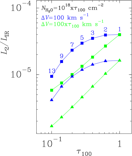
Figure 10: Modeled $L_{\mathrm{2}}/L_{\mathrm{IR}}$ ratio as a function of $\tau_{100}$. Squares and triangles indicate $T_{\mathrm{dust}}=55$ and $75$ K, respectively. In all models, collisional excitation is included with $T_{\mathrm{gas}}=150$ K and $n_{\mathrm{H_{2}}}=3\times 10^{4}$ cm^-3. $N_{\mathrm{H_{2}O}}/\tau_{100}=10^{18}$ cm^-2 is adopted, corresponding to a constant H₂O abundance of $7.7\times 10^{-7}$ (Eq. 1). Blue symbols indicate models with $\Delta V=100$ km s^-1 and thus with variable $K_{\mathrm{vir}}$ (Eq. 5) indicated with the numbers. Green symbols show results with $\Delta V=100\times\tau_{100}$ km s^-1 simulating a constant value of $K_{\mathrm{vir}}=1.3$. When compared with observations, the modeled $L_{\mathrm{IR}}$ values should be considered a fraction of the observed IR luminosities (Sect. 4.3.1), and thus the modeled $L_{\mathrm{2}}/L_{\mathrm{IR}}$ values are upper limits.

The broad range in observed $L_{\mathrm{IR}}$ in luminous IR galaxies with H₂O emission may be attributable to varying the effective size of the emitting region. As noted in Sect. 3.2, varying $R_{\mathrm{eff}}$ (equivalent to varying the number of individual regions that contribute to $L_{\mathrm{IR}}$ or to increasing $L_{\mathrm{IR}}$ for a single source) is expected to generate linear $L_{\mathrm{H_{2}O}}-L_{\mathrm{IR}}$ correlations if the other parameters ($T_{\mathrm{dust}}$, $\tau_{100}$, $T_{\mathrm{gas}}$, $n_{\mathrm{H_{2}}}$, $N_{\mathrm{H_{2}O}}/\Delta V$, and $\Delta V$) remain constant.

In Fig. 10 we show the $L_{2}/L_{\mathrm{IR}}$ ratio as a function of $\tau_{100}$ for models with $T_{\mathrm{dust}}=55$ K and $T_{\mathrm{dust}}=75$ K that assume a constant H₂O-to-dust opacity ratio, that is, $N_{\mathrm{H_{2}O}}/\tau_{100}=10^{18}$ cm^-2. According to Eq. (1), this corresponds to a constant H₂O abundance of $7.7\times 10^{-7}$. Both models with $\Delta V=100$ km s^-1 (independent of $\tau_{100}$), and $\Delta V/\tau_{100}=100$ km s^-1 (corresponding to a constant $K_{\mathrm{vir}}=1.3$) are shown. The figure illustrates that a supralinear correlation between $L_{\mathrm{H_{2}O}}$ and $L_{\mathrm{IR}}$ can be expected if, on average, $\tau_{100}$ is an increasing function of $L_{\mathrm{IR}}$. If most sources with $L_{\mathrm{IR}}\sim 5\times 10^{10}$ L_⊙ were optically thin ($\tau_{100}\sim 0.1$), and the high-$z$ sources with $L_{\mathrm{IR}}\sim 10^{13}$ L_⊙ (O13) were mostly optically thick ($\tau_{100}\sim 1$), one would then expect $L_{2}\propto L_{\mathrm{IR}}^{1.3}$ from Fig. 10, which can account for the observed supralinear correlation found by O13 and Y13. However, similar supralinear correlations would then be expected for the other submm lines $3-6$.

5 Summary of the model results for optically classified starbursts and AGNs

Following the optical classification of sources by Y13 into optically classified star-formation-dominated galaxies with possible mild AGN contribution (HII+mild AGN sources) and optically identified strong-AGN sources, we now consider these two groups separately.

5.1 HII+mild AGN sources

We focus here on those HII+mild AGN sources where lines $2-6$ are detected but lines $7-8$ are undetected (that is, “warm” sources as defined in Sect. 4.1). The average H₂O flux ratios reported by Y13 (their Table 2) indicate that $(i)$ $F_{6}/F_{2}\sim 1.2$, favoring $T_{\mathrm{dust}}=55$ K if there is no significant collisional excitation and $T_{\mathrm{dust}}=75$ K if the H₂O emission arises in warm and dense gas (Fig. 5); $(ii)$ $F_{6}/F_{5}\sim 1.2$, consistent with the optically thin regime (Fig. 6). For these $T_{\mathrm{dust}}$, Fig. 11a shows the values of $N_{\mathrm{H_{2}O}}$ for $\Delta V=100$ km s^-1 required to explain the observed $L_{\mathrm{H_{2}O}}/L_{\mathrm{IR}}$ ratios, as a function of $\tau_{100}$. Models with included or excluded collisional excitation are considered. We recall that $\Delta V$ is the velocity dispersion of the dominant structure(s) that accounts for the H₂O emission (Sect. 3.2), and for the case of low $\tau_{100}$ and relatively high densities, Eq. (6) suggests $\Delta V<100$ km s^-1 with the consequent increase in $N_{\mathrm{H_{2}O}}$ (Fig. 10).

The decrease in $\tau_{100}$ implies the increase in $N_{\mathrm{H_{2}O}}$ in optically thin conditions and when collisional excitation is unimportant. Our best fit models for the average SLED (big solid symbols) favor optically thin far-IR emission ($\tau_{100}\lesssim 0.3$). In Fig. 11b-e, the detailed comparison between the $\tau_{100}=0.1$ models and the observations (Y13) is shown. Significant collisional excitation is not favored for $T_{\mathrm{dust}}=55$ K, since it would increase $F_{2}$ relative to $F_{6}$. In addition, these optically thin models have the drawback of overestimating $F_{4}/F_{2}$. Conversely, the $T_{\mathrm{dust}}=75$ K models favor significant collisional excitation in order to increase $F_{2}$ relative to $F_{6}$. The very optically thin models ($\tau_{100}\lesssim 0.05$) are also not favored given the very high amounts of H₂O required to explain (with no collisional excitation) the $L_{\mathrm{H_{2}O}}/L_{\mathrm{IR}}$ ratios.

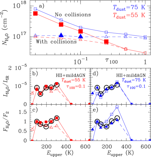
Figure 11: a) Values of $N_{\mathrm{H_{2}O}}$ for $\Delta V=100\,\mathrm{km\,s^{-1}}$ as a function of $\tau_{100}$, for $T_{\mathrm{dust}}=55$ K (red) and $75$ K (blue), required to account for the observed averaged $L_{\mathrm{H_{2}O}}/L_{\mathrm{IR}}$ ratios in HII-mild AGN sources (as given by Y13). Models both without (squares) and with (triangles) collisional excitation are shown. In the latter models, $T_{\mathrm{gas}}=150$ K, and $n_{\mathrm{H_{2}}}=5\times 10^{4}-3\times 10^{5}$ cm^-3 for $T_{\mathrm{dust}}=55-75$ K, respectively. The large filled symbols indicate the best fit models to the averaged SLED. Panels b-e) compare in detail the four models with $\tau_{100}=0.1$ (both with and without collisions) with the observed values (black circles) in HII-mild AGN sources (both the normalized flux ratios (SLED) and the $L_{\mathrm{H_{2}O}}/L_{\mathrm{IR}}$ ratios, Y13, for lines 2-6). In panels b) and d), the models indicate the values of $L_{\mathrm{H_{2}O}}/L_{\mathrm{IR}}$ for $\Delta V=100$ km s^-1. Lines 1, 7, and 8 are excluded from the comparison because of their low detection rates (Y13).

In summary, $T_{\mathrm{dust}}=55-75$ K, $\tau_{100}\sim 0.1$, and $N_{\mathrm{H_{2}O}}\sim(0.5-2)\times 10^{17}$ cm^-2 can explain the bulk of the H₂O submm emission in warm star-forming galaxies (Table 2). As shown in Fig. 8, $T_{\mathrm{dust}}=55$ K and $\tau_{100}=0.1-0.2$ predict 25-to-60 $\mu$m flux density ratios of $f_{25}/f_{60}=(8.5-6.0)\times 10^{-2}$, in agreement with the observed values for the bulk of sources (Y13), while $T_{\mathrm{dust}}=75$ K and $\tau_{100}=0.1-0.2$ predict $f_{25}/f_{60}=0.42-0.30$ (close to the observed upper values). Assuming a gas-to-dust ratio of 100 by mass, $\tau_{100}\sim 0.1$ corresponds to a column density of H nuclei of $N_{\mathrm{H}}\approx 1.3\times 10^{23}$ cm^-2 (Eq. 1), and thus an H₂O abundance of $X_{\mathrm{H_{2}O}}\sim 10^{-6}$. To within a factor of 3 uncertainty due to the $\tau_{100}-N_{\mathrm{H}}$ calibration, the specific values used for $\tau_{100}$ and $\Delta V$, and variations in the measurements for individual sources, this is the typical H₂O abundance that we infer from the observed $L_{\mathrm{H_{2}O}}-L_{\mathrm{IR}}$ correlation. Molecular shocks and hot core chemistry are very likely responsible for this $X_{\mathrm{H_{2}O}}$, which is well above the volume-averaged values inferred in Galactic dark clouds and PDRs (e.g., Bergin et al., 2000; Snell et al., 2000; Melnick & Bergin, 2005; van Dishoeck et al., 2011).

Finally, we note that $T_{\mathrm{dust}}=55$ K and $\tau_{100}=0.1-0.2$, and the assumption that most of the IR is powered by star formation in these sources of Y13, imply a star-formation-rate surface density of $\Sigma_{\mathrm{SFR}}=121-195$ M_⊙ yr^-1 kpc^-2 and gas mass surface density of $\Sigma_{\mathrm{gas}}=1430-2860$ M_⊙ pc^-2. The implied depletion or exhaustion time scale, $t_{\mathrm{dep}}=\Sigma_{\mathrm{gas}}/\Sigma_{\mathrm{SFR}}$, is $\sim 12-15$ Myr. These values lie close to the $\Sigma_{\mathrm{SFR}}-\Sigma_{\mathrm{dense}}$ star-formation correlation found by García-Burillo et al. (2012) from HCN emission in (U)LIRGs with their revised HCN-$M_{\mathrm{dense}}$ conversion factors. This agreement suggests that the submm H₂O and the mm HCN emission in (U)LIRGs arise from the same regions. Sources with $T_{\mathrm{dust}}=75$ K would imply even shorter time scales and suggest high rates of ISM return from SNe and stellar winds. A follow-up study of the relationship between $L_{\mathrm{H_{2}O}}$ and $L_{\mathrm{HCN}}$ is required to check this point. In addition, modeling the individual sources simultaneously in the continuum and the H₂O emission will provide further constraints on the nature of these regions.

5.2 Strong optically classified AGN sources

The general finding that the H₂O emission is similar in star-forming and strong-AGN sources (Y13) may simply indicate that the far-IR pumping of H₂O occurs regardless of whether the dust is heated via star formation or an AGN. There are, however, some differences between the two source types. Strong AGNs show a higher detection rate in H₂O $1_{11}-0_{00}$ (Y13), indicating that the gas densities are higher in the circumnuclear regions of AGNs. Another difference is that the $L_{\mathrm{H_{2}O}}/L_{\mathrm{IR}}$ ratios are somewhat lower in strong AGN sources (Y13). While relatively low columns of dust and H₂O in these sources could explain this observational result, it is also possible that high X-ray fluxes photodissociate H₂O, reducing its abundance relative to star-forming galaxies. High abundances of H₂O require effective shielding from UV and X-ray photons and thus high columns of dust and gas that, in AGN-dominated galaxies, may be effectively provided by an optically thick torus probably accompanied by starburst activity. In addition, warm dust further enhances $X_{\mathrm{H_{2}O}}$ through an undepleted chemistry and pumps the excited H₂O levels, while warm gas will further boost $X_{\mathrm{H_{2}O}}$ through reactions of OH with H₂. These appear to be the ideal conditions for the presence of large quantities of H₂O in the (circum)nuclear regions of galaxies.

Appendix A Two opposite, extreme cases: Arp 220 and NGC 1068

Arp 220 and NGC 1068 are prototypical sources that have been observed at essentially all wavelengths. With regard to their H₂O submm emission, these galaxies are extreme cases and deserve special consideration.

In the nearby ULIRG Arp 220, discrepancies between the observed SLED (Rangwala et al., 2011, Y13) and the single-component models of Fig. 3a1-c1 are worth noting. The observed high $L_{6}/L_{\mathrm{IR}}\approx 2.4\times 10^{-5}$ (Fig. 8), together with the high 6/2 ratio of $\approx 1.4$ (Fig. 12a), suggest $T_{\mathrm{dust}}\gtrsim 65$ K and $N_{\mathrm{H_{2}O}}\gtrsim 10^{17}$ cm^-2, consistent with detection of lines $7-8$. However, high $T_{\mathrm{dust}}$ and $N_{\mathrm{H_{2}O}}$ are mostly compatible with $F_{4}/F_{3}>1$, while the observed ratio is $\approx 0.7$ (Fig. 12a). As in Mrk 231, a composite model is required to account for the H₂O SLED in this galaxy.

In sources with very optically thick and very warm cores such as Arp 220 (G-A12), the increase in $\tau_{100}$ above 1 decreases the submm H₂O fluxes due to the rise of submm extinction (Fig. 9). While higher $T_{\mathrm{dust}}$ generates warmer SEDs, but lowers the $L_{\mathrm{H_{2}O}}/L_{\mathrm{IR}}$ ratios for lines $2-6$, the increase in $\tau_{100}$ further decreases $L_{\mathrm{H_{2}O}}/L_{\mathrm{IR}}$. This behavior suggests that the optimal environments for efficient H₂O submm line emission are regions with high far-IR radiation density but moderate extinction, i.e., those that surround the thick core(s) where the bulk of the continuum emission is generated. In contrast, the H₂O absorption at shorter wavelengths is more efficiently produced in the near-side layers of the optically thick cores, primarily if high-lying lines are involved. Absorption and emission lines are thus complementary, providing information on the source structure.

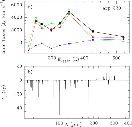
Figure 12: a) Proposed composite model for the H₂O submm lines in Arp 220 (see G-A12), compared with the observed line fluxes (black squares, from Rangwala et al., 2011). Toward the far-IR optically thick nuclear region (blue symbols), the $E_{\mathrm{upper}}<400$ K lines are expected mostly in absorption. The H₂O emission is generated around that nuclear region, in the $C_{\mathrm{extended}}$ (G-A12) component (green). Red is total. b) Resulting predicted composite PACS/SPIRE H₂O continuum-subtracted spectrum of Arp 220, which is dominated by absorption of the continuum.

We have taken the models in G-A12 for Arp 220 to predict its submm H₂O emission. In Fig. 12a, the blue symbols/line indicate the predicted H₂O fluxes towards the optically thick, warm nuclear region (both $C_{\mathrm{west}}$ and $C_{\mathrm{east}}$, see G-A12), indicating that most submm lines (with the exception of lines 3, 7, and 8) are predicted in absorption. The observed H₂O submm line emission (Rangwala et al., 2011) must therefore arise in the surrounding, optically thinner region, i.e., the $C_{\mathrm{extended}}$ component, where the H₂O abundance in the inner parts ($R\lesssim 150$ pc, where $T_{\mathrm{dust}}=70-90$ K) is increased relative to G-A12 (so $C_{\mathrm{extended}}$ has $N_{\mathrm{H_{2}O}}=1.3\times 10^{17}$ cm^-2 in Fig. 12a). According to our model, the relatively low flux in line 4 is due to line absorption towards the nuclei. The main drawback of the model in Fig. 12a is that line 7 is underestimated by a factor 2. The submm H₂O emission in Arp 220 traces a transition region between the compact optically thick cores and the extended kpc-scale disk (G-A12). The overall H₂O spectrum is, however, dominated by absorption of the continuum (Fig. 12b).

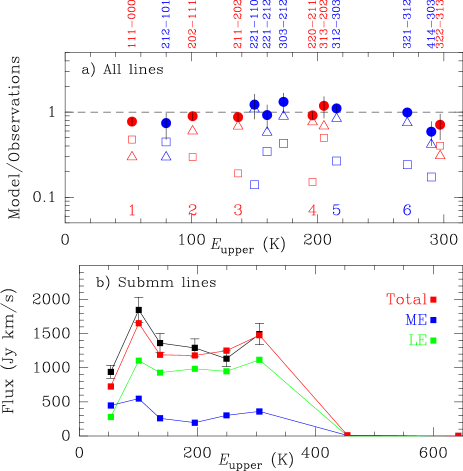
Figure 13: a) Composite model for the H₂O emission in NGC 1068 favored in this work. Blue/red indicate ortho/para lines, and the submm H₂O $1-6$ lines (Table 1) are indicated. Open squares and triangles show the contribution by a moderate-excitation (ME) and a low-excitation (LE) component, and filled symbols indicate the total emission (see text for details); in both cases the submm H₂O lines $2-6$ are pumped through far-IR photons emitted by dust. b) Comparison between the observed fluxes of the H₂O submm lines (black squares, from Spinoglio et al., 2012) and those predicted with the composite model.

Just the opposite set of conditions characterizes the nearby Seyfert 2 galaxy NGC 1068, since the nuclear continuum emission is optically thin and collisional excitation is important (S12). All detected H₂O lines, including those in the far-IR ($100-200$ $\mu$m) are seen in emission, and most of them show fluxes (in erg/s/cm²) unrelated to wavelength, upper level energy (up to $\approx 300$ K), or $A$-Einstein coefficient (S12). In particular, the H₂O $2_{21}-1_{10}$ (108 $\mu$m) and $2_{21}-2_{12}$ (180 $\mu$m) lines share the same upper level and show similar fluxes but the $A$-Einstein coefficient of the 108 $\mu$m transition is a factor of $8.4$ higher than that of the 180 $\mu$m transition. With pure collisional excitation, the only way to account for the observed line ratios is to invoke high densities and H₂O column densities, but also a relatively low $T_{\mathrm{gas}}$ to avoid significantly populating the high-lying levels ($>300$ K). S12 found that $T_{\mathrm{gas}}\sim 40$ K, and very high $N_{\mathrm{H_{2}O}}$ and $n_{\mathrm{H_{2}}}$ can provide a reasonable fit to the SLED. However, these conditions are unrelated to the warmer gas conditions in the nuclear region of NGC 1068, as derived from the CO SLED (S12, Hailey-Dunsheath et al., 2012, hereafter H12). In addition, the observed H₂O submm SLED (Fig. 13) is fairly similar to the SLEDs obtained in optically thin models with significant collisional excitation of the low-lying levels.

We have explored an alternative composite solution for the H₂O emission in NGC 1068 with lower densities and H₂O columns and higher $T_{\mathrm{gas}}$, based on the far-IR pumping of the lines by an external anisotropic radiation field. In this framework, we can account for the weakness of the 108 $\mu$m line by the absorption of continuum photons, and indeed we would have to explain why this line is not observed to be even weaker than it is or in absorption. The higher lying far-IR $3_{22}-3_{13}$ emission line at $156.2$ $\mu$m is in this scenario pumped through absorption of continuum photons in the $3_{22}-2_{11}$ line at 90 $\mu$m.

For the first component, we closely follow H12 in modeling the moderate-excitation (ME) component as an ensemble of clumps, which are described by $T_{\mathrm{dust}}=55$ K, $\tau_{100}=0.18$, $n_{\mathrm{H_{2}}}=10^{6}$ cm^-3, $T_{\mathrm{gas}}=150$ K, and $N_{\mathrm{H_{2}O}}=6.5\times 10^{16}$ cm^-2, and $V_{\mathrm{turb}}=15$ km s^-1 (giving $K_{\mathrm{vir}}\sim 10$, see H12). With a mass of $7.5\times 10^{6}$ M_⊙, this component is unable to account for the H₂O submm lines $2-6$, but generates a significant fraction of the observed emission in line 1 and some far-IR lines (Fig. 13a and panel b).

We then added another, low-excitation (LE) component, which is identified with the gas generating the low-$J$ CO lines (Krips et al., 2011, S12) and is thus assigned a density of $n_{\mathrm{H_{2}}}=2\times 10^{4}$ cm^-3. For simplicity, we also assume $T_{\mathrm{dust}}=55$ K, $\tau_{100}=0.18$, and $N_{\mathrm{H_{2}O}}=6.5\times 10^{16}$ cm^-2 as for the ME, but adopt the higher $V_{\mathrm{turb}}$ of $60$ km s^-1 (giving $K_{\mathrm{vir}}\sim 7$). For the LE component, and besides the internal far-IR field described by its $T_{\mathrm{dust}}$ and $\tau_{100}$, we also follow H12 in including an external field (associated with the emission from the whole region), which is described as a graybody with $T_{\mathrm{BG}}=55$ K and $\tau_{100}^{BG}=0.05$. The resulting mean specific intensity at 100 $\mu$m of the external field, $J_{\mathrm{ext}}^{100\mu\mathrm{m}}$, matches the value estimated by H12 within a factor of 2 (their Eq. 1). A crucial aspect of the present approach is that this external field is assumed to be anisotropic, that is, it does not impinge into the LE clumps on the back side (in the direction of the observer). As a result, the external field contributes to the H₂O excitation without generating absorption in the pumping far-IR lines (though some absorption is nevertheless produced by the internal field). As shown in Fig. 13a, the LE component is expected to dominate the emission of the submm lines $2-6,$ as well as the emission of the majority of the far-IR lines. The required mass of the LE component is $3.5\times 10^{7}$ M_⊙, consistent with the mass inferred from the CO lines for the CND (S12), and the IR luminosity is $2.6\times 10^{10}$ L_⊙.

A key assumption of the present model is that the external radiation field does not produce absorption in the far-IR lines, as otherwise (that is, in a perfectly isotropic radiation field) the strengths of the far-IR lines would weaken, and in particular, the H₂O $2_{21}-1_{10}$ line at 108 $\mu$m line would be predicted to be observed in absorption. The proposed anisotropy could be associated with the heating by the central AGN, and it seems possible as long as the source is optically thin in the far-IR. Radiative transfer in 3D would be required to check this feature. On the other hand, the external field, while having an important effect on the far-IR lines, has a secondary effect on the submm lines, which are primarily pumped by the internal (isotropic) radiation field (that is, by the dust that is mixed with H₂O). With the caveat of the assumed intrinsic radiation anisotropy in mind, we preliminary favor this model over the pure collisional one in predicting the H₂O submm fluxes and conclude that radiative pumping most likely plays an important role in exciting the H₂O in the CND of NGC 1068.

From the models for these two very different sources and the case of Mrk 231 studied previously (G-A10), we conclude that the excitation of the submm H₂O lines other than the $1_{11}-0_{00}$ one is dominated by radiative pumping, though the relatively low-lying $2_{02}-1_{11}$ line may still have a significant “collisional” contribution in some very warm/dense nuclear regions, and the radiative pumping may be enhanced with collisional excitation of the low-lying $1_{11}$ and $2_{12}$ levels. These individual cases also show that composite models to account for the full H₂O far-IR/submm spectrum in a given source may be a rather general requirement.