Automatic data analysis for Sky Brightness Monitor

Abstract

The Sky Brightness Monitor (SBM) is an important instrument to measure the brightness level for the sky condition, which is a critical parameter for judging a site for solar coronal observations. In this paper we present an automatic method for the processing of SBM data in large quantity, which can separate the regions of the Sun and the nearby sky as well as recognize the regions of the supporting arms in the field of view. These processes are implemented on the data acquired by more than one SBM instruments during our site survey project in western China. An analysis applying the result from our processes has been done for the assessment of the scattered-light levels by the instrument. Those results are considerably significant for further investigations and studies, notably to derive a series of the other important atmospheric parameters such as extinctions, aerosol content and precipitable water vapor content for candidate sites. Our processes also provide a possible way for full-disk solar telescopes to track the Sun without an extra guiding system.

1 Introduction

The sky brightness is a critical parameter for judging a potential site for direct coronal observation. Due to the large difference in the brightness of the solar disk and its nearby sky (halo), it is difficult to achieve the accurate and direct measurement of the sky brightness during the day time. The corona can only be observed during total solar eclipses until the Lyot coronagraph was invented (Lyot, 1930, 1939). Afterwards, a photometer for measurement of sky brightness near the Sun is constructed by Evans (1948). Evans Sky Photometer (ESP) has been used for a long time at various solar observatories (Garcia and Yasukawa, 1983; Labonte, 2003). A modern Sky Brightness Monitor (SBM) has been developed for the Advanced Technology Solar Telescope (ATST) site survey project, which can image the solar disk and the nearby sky simultaneously at 450, 530, 890 and 940 nm (Penn et al., 2004; Lin and Penn, 2004). In addition, the SBM data can yield information about the extinction, the aerosols, and the precipitable water vapor content of the atmosphere.

To meet the future development of the Chinese Giant Solar Telescope (CGST) and large-aperture coronagraphs projects, our SBM is designed and developed following the same idea from Lin and Penn (2004), as one fundamental tool (Liu et al., 2012b). These SBMs have been applied at many different candidate sites up to now (Liu et al., 2011, 2012a, 2012b). The optical configuration of one SBM consists of an external occulter, an objective lens, a neutral density filter on the objective lens, and the four bandpass filters (Lin and Penn, 2004). Generally, the original images acquired by the SBM are not intuitional and concise for a directly further analysis. Moreover, the absence of an auto guide system to serve the equatorial tracking system would result in an indeterminateness of the positions of the solar disk in the SBM’s images. Wen et al. (2012) studied and compared the possible methods for determining the solar disk center in SBM’s data. However, they could not break away from the constraint of some experienced parameters which need personnel intervention. Furthermore, the invalid regions for calculating the sky brightness are excluded manually in former work, too(Liu et al., 2012b). With the rapid progress of our site survey project, the accumulation of huge amounts of data urgently necessitates an efficient, accurate and a fully automated processing approach to deal with the SBM data.

For this purpose, we have developed a method for automatically processing the SBM data, which allows separating the regions of the Sun and the nearby sky as well as permits to automatically recognize the regions of the supporting arms. In the next section, we describe the main adopted technologies for our procedure. In Section 3, we present the data reduction in detail. In Section 4, we apply our procedure on a set of SBM’s data and analyze the scattered light based on the results of our procedure. Our conclusions are presented and highlighted in Section 5.

2 Main Technologies

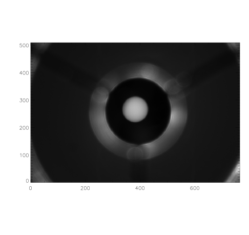
Figure 1: A typical SBM image taken at Gaomeigu Station in Lijiang city. X- and Y- directions represent the two dimensions of the image in pixels, similarly hereafter.

The SBM instruments can simultaneously image the Sun and its nearby sky regions. The data is useful for directly deducing the normalized sky brightness which is a critical parameter for coronagraph site investigation. Fig. 1 shows a typical SBM image taken at Gaomeigu Station. Near the center of the image, the attenuated solar disk and the projection of the ND4 (nominal optical density of 4) filter are shown. The bright ring is caused by the diffraction at the edge of the ND4 filter, while the three narrow strips are from the projections of the supporting arms of the ND4 filter.

The brightness of the sky within a few solar radii away from the solar center at a good coronal site is expected to be below $10^{-5}\times I_{\odot}$, where $I_{\odot}$ is the intensity of the solar disk (Lin and Penn, 2004). It is convenient to measure the sky brightness with millionths of $I_{\odot}$. In order to extract the regions of the solar disk and the Sun’s nearby sky, it is necessary to accurately determine the solar radius and the position of the solar center in the image. Because the region of the Sun’s nearby sky on the image contains the projections of the supporting arms which must be excluded in the calculation, the accurate positions of these projections are also needed for each image. In our procedure, there are mainly three technologies used to achieve the separation of these regions: image binarization with Otsu’s method, image matching with cross-correlation, and image fitting with the method of least-squares.

In digital image processing, Otsu’s method is usually used to automatically perform clustering-based image binarization. The algorithm assumes that the image contains two classes of pixels corresponding to two peaks on its histogram (foreground and background). The optimum threshold to separate those two classes is calculated by minimizing their combined spread (intra-class variance) (Otsu, 1979).

In Otsu’s method, the intra-class variance (the variance within the class) is defined as a weighted sum of variances of the two classes:

$$\sigma^{2}(T)=\omega_{1}(T)\sigma_{1}^{2}(T)+\omega_{2}(T)\sigma_{2}^{2}(T)$$ (1)

where $\omega_{i}$ are the probabilities of the two classes separated by a threshold $T$ and $\sigma^{2}_{i}$ are variances of these classes.

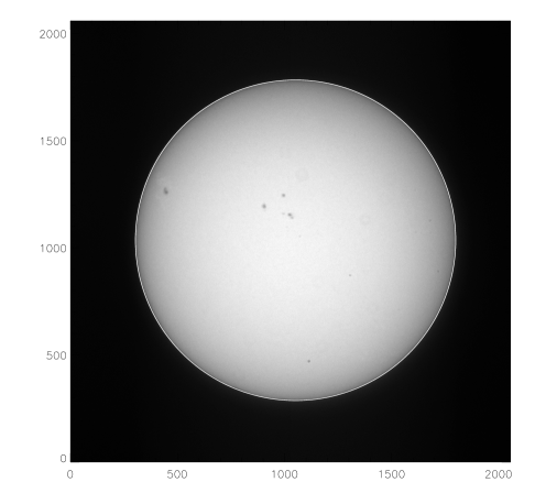
Figure 2: An illustration of image binarization based on Otsu’s method. The image is taken at Full-Shine lake in Yunnan. (a) is a whitelight solar image. (b) is the result applying Otsu’s method on (a). (c) is the binarized image based on the threshold from (b). (d) shows the boundary of (c) superimposed on (a).

In this step, the image is re-scaled to 8-bit and the normalized histogram is calculated. Then we test all the possible thresholds T from 0 to 255 to calculate the intra-class variances and find the desired T in the 256 thresholds. At last, the actual threshold for the origin image is obtained by an inverse scaling mapping. For example, applying Otsu’s method on a white light solar image would locate the boundary with a high accuracy (Fig. 2). In our procedure, Otsu’s method is mainly used for the edge detecting of the SBM image.

Correlation techniques is predominately used for template matching in image processing (Gonzalez and Woods, 2002). If we want to determine whether an image $f(x,y)$ containing a particular object or region of interest, we let $h(x,y)$ be that object or region (template). Then, if there is a match, the correlation of the two functions will be maximum at the location where $h(x,y)$ finds a correspondence in $f(x,y)$.

Cross-correlation of two continuous functions f and h is defined as

$$f(t)\circ h(t)=\int_{-\infty}^{\infty}f^{\ast}(\tau)h(t+\tau)d\tau$$ (2)

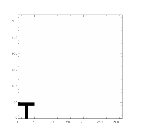
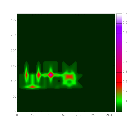
Figure 3: A simple illustration of image correlation. It is constructed following the example 4.41 in Gonzalez and Woods (2002).(a) is the image and (b) is the template. (c) shows the cross correlation between (a) and (b). (d) is the horizontal profile line through the highest value in (c).

where the asterisk denotes the complex conjugate of $f$. If $f$ and $h$ are real valued functions, this formula essentially slides the function $h$ a displacement to function $f$ and calculates the integral of their product at each position. When the functions match, the value of $f\circ h$ is maximized. This is because when peaks (or troughs) are aligned, they make a large contribution to the integral. With complex valued functions $f$ and $h$, taking the conjugate of $f$ ensures that aligned peaks (or aligned troughs) with imaginary components will contribute positively to the integral. Therefore, one can use the cross-correlation to find how much $h$ must be shifted to make it identical to $f$. An illustrating example is shown in Fig. 3. In our procedure, cross-correlation is used for edge extracting and to determine the positions of the supporting arms.

The method least-squares (LSQ) is extensively utilized in data fitting. It is a standard approach to the approximate solution of over-determined systems, in which the number of measurements is more than that of unknown variables. Least-squares means that it minimizes the sum of the squared residuals. In our procedure, least-squares is used to fit the circles by the points of the edges of the solar disk and the ND4 filter.

For a circle with the algebraic equation,

$$F(x_{i},y_{i},\vec{\beta})=a(x_{i}^{2}+y_{i}^{2})+b_{1}x_{i}+b_{2}y_{i}+c=0,$$ (3)

determining the parameters ($\vec{\beta}=[a,b_{1},b_{2},c]$) of the algebraic equation in the least-squares sense is called algebraic fit, while minimizing the sum of the squares of the distances to the center point

$$d_{i}^{2}=(\|\vec{z}-\vec{x}_{i}\|-r)^{2}$$ (4)

is called geometric fit, where $\vec{z}$ is the center coordinate of the circle and $r$ is the radius of the circle (Gander et al., 1994). The sum of the squared residuals of the distance function is obviously a non-linear function. Therefore, we solve this non-linear least-squares problem iteratively with the Gauss-Newton method. And the algebraic solution is used as the starting vector for the iteration. An example is shown in Fig. 4. The results of the algebraic and the geometric fits are very different. For fitting analysis of data, the algebraic fit only tries to find the curve which minimizes the vertical displacement while the geometric fit tries to minimize the orthogonal distance. On this account, geometric fit sometimes is mentioned as ”best fit”, because it can provide more aesthetic and accurate results.

3 Description of the Data Reduction

The positions of the solar disk in a time sequence are crucial parameters for the sky brightness calculations. Due to the actual operation on the instrument, the solar image center is usually shifted around the center of the ND4 filter. Because the two ND2 filters are fixed on the supporting arms, the position of the center and the projection size of the filters are also important parameters for the calculations.

3.1 Data selection

In actual observations, there may be a lot of data that are mistakenly collected due to the observational constraints. Because the SBM is a portable measurement designed for field observations, the weather condition has a great influence on the acquired images. Moreover, in the absence of a guiding system and high-precision tracking system, the SBM often gathers bad images in which the Sun moves out of the field of view. Hence a data selection program must be performed prior to any further calculations.

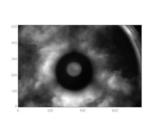
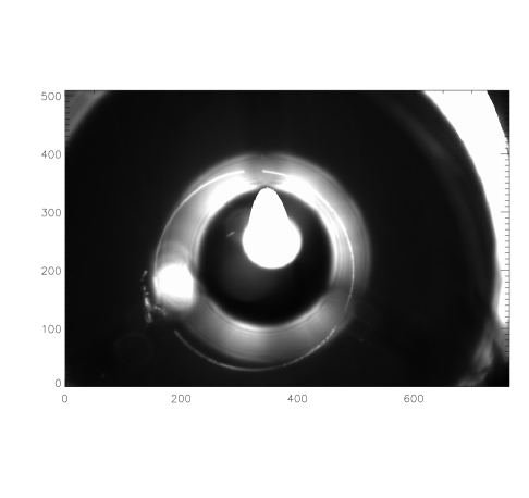
Figure 5: (a) represents the bad image covered by clouds. (b) represents the bad image, clearly saturated.

There are mainly two types of bad data in the observation which are represented in Fig. 5. Fig. 5 (a) represents the bad image covered by the clouds and (b) shows the bad image which is saturated. We use an operation on experiential thresholds to recognize these situations. Binary operations are applied to the images according to the thresholds by Otsu’s method and 0.999 maximum, respectively. Then the areas of the binarization images are calculated. Because Otsu’s threshold separates two typical classes of pixels optimally and the clouds attenuation the differences of these two classes, the areas from Otsu’s threshold will be very large. And if the image is saturated, there will be too many pixels with values identical to the maximum. Hence the area from 0.999 maximum threshold will be too large. We note that these two criteria are not independent. For example, when the weather is seriously cloudy, the image will be saturated in large area, and the binarization images based on Otsu’s threshold and 0.999 maximum threshold are nearly the same.

We also take into account some other ordinary situations such as for the Sun totally out of the field of view. Our data selection procedure is very effective to automatically get rid of those data. This has been verified based on all the SBM’s data, collected in 2013, during the solar site survey. However the accurate thresholds can not be given because our criteria depend on the experience. In fact, we adopt a slight strict threshold to ensure the selecting to be sufficient while a very few regular data will be excluded improperly.

3.2 Edge detection and extraction

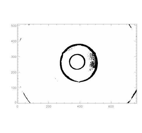
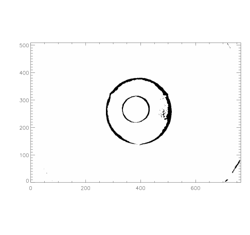
Figure 6: (a) is the enhanced image, which is the logarithm of the initial image . (b) is the gradient of image (a) by Sobel operator. (c) is the binarized image based on the threshold from (b). (d) is the eroded image of (c) by morphological method. We note that the gray levels of the binarized images are inverted for display, similarly hereafter.

The second step in our procedure is edge detection. We apply Sobel operator on the enhanced SBM image to get the gradient image and use Otsu’s Method to threshold the gradient image. Then the edge of the solar disk combined with that of the ND4 filter and some other small structures are obtained (see Fig. 6). Here a morphological erosion with a circular structuring element of $7\times 7$ pixels is employed to make the edge more distinct.

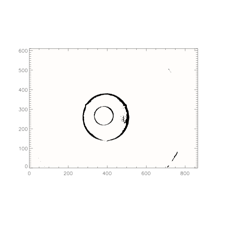
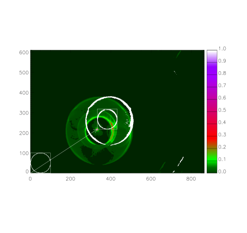
Figure 7: (a) is the padded edge image. (b) is the padded template. (c) is the cross-correlation between (a) and (b). (d) is the superimposed image of (a), (b) and(c).

The subsequent step consists of extracting the edge of the solar disk and of the ND4 filter from the respectively detected edges. This step is achieved through image-matching based on cross-correlation. For the solar disk, the angular diameter can be obtained from the recording time of the image. Combining with the focal length of the SBM, we can gain the theoretical size of the solar diameter on the image. By taking into account the size of CCD element, we finally get the solar diameter in pixels. Then the template for cross-correlation can be constructed. Indeed, a 5-pixels width ring is constructed and adopted as the template instead of a simplified circle template. The results are shown in Fig. 7. The image and template are padded to avoid wraparound error. The maximum of the resulted correlation-image highlights the displacement with which the template should be shifted. According to this recovered displacement and the size of the template, the edge of the solar disk can be extracted from the image reported in Fig. 6. Afterwards, by applying the least-square approach we fit the circle using the edge points of the solar disk to accurately estimate the coordinates of solar center and radius. Similar procedures are performed on the edge of the ND4 filter.

For the solar disk analyses, the cross-correlation technique might give wrong displacement. In some situations, there is so much scattered light between the solar disk and the inner edge of the ND4 filter (diffraction ring) that the thresholding image from Otsu’s Method might give ambiguous edges therein. Consequently, when the template is shifted to the position where the scattered light is evident, the correlation coefficient is significantly amplified. To overcome this, we proceed by calculating the convolution of the image-of-correlation and the corresponding Laplacian Kernel function. It turns out that the correlation maximum of the defective image-of-correlation is effectively reduced after convolution. It is noted that in the case of the ND4 filters, there is no similar problem found.

3.3 Locating the position of the supporting arms

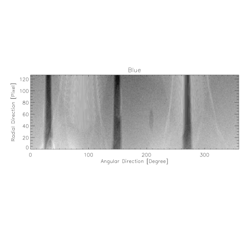
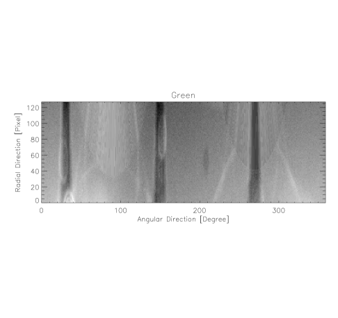
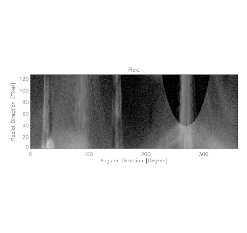
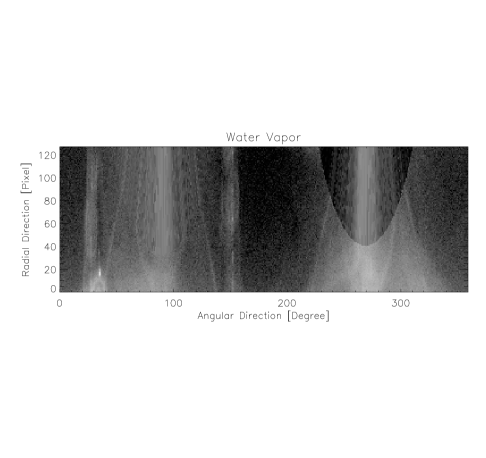
Figure 10: The expanding sky regions at different wavelengths. The parabolic regions are the annular regions out of the image constructed by interpolating with the points on the edge.

Considering the regions of the supporting arms’ projections could not be used for the sky brightness calculations, one needs hence to get rid of these regions. For this purpose we test the cross-correlation technique to locate the position of the supporting arms. However, it can not be applied directly because the template with invariable characteristics is hardly to be constructed. Moreover, as long as the supporting arms are fixed on the ND4 filter, we can use the center of the ND4 filter as the pole to expand the image in polar coordinate system. As shown in Fig. 10, an annular region out of the diffraction ring is isolated and expanded. The expanded image reveals a clear distinctive feature, namely, three parallel strips with $120^{\circ}$ away from each other.

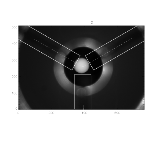
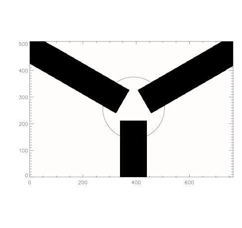
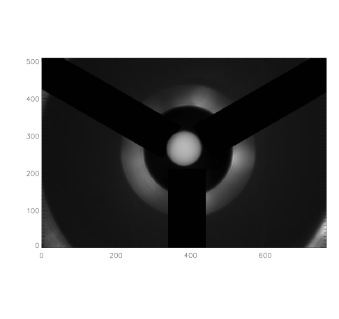
Figure 11: (a) is the SBM image. (b) is the mask. (c) is the product of (a) and (b). (d) shows the solar disk and the sky regions.

Worthy of note, for convenience we inverse the values of the expanded image. Because the projections of the supporting arms in the expanded images are relatively fixed and parallel, a two-column template can work well enough. Moreover, the sky brightness is not uniform at the angular direction, the template constructed adopting two Gaussian functions is more suitable than using three Gaussian functions. Due to our concerning only the positions of the supporting arms on the angular direction, the template needs not to be designed too high. On consideration of the efficiency, we eventuality adopt a template consists of two Gaussian functions aligned with their maximums at a distance of $120^{\circ}$ and with a width of 32 pixels. The results are illustrated in Fig. 11.

The SBM instrument measures the solar disk and sky brightness at four wavelengths, including 450 nm, 530 nm, 890 nm and one at the water vapor absorption band of 940 nm. The data acquisition system is collecting images at four wave bands in the sequence of wavelengths. The scattered light of the sky might be found weaker than that of the supporting arms especially in some cases when the sky brightness is too weak. An example is depicted in Fig. 12. In this situation, the images at 890 and 940 nm will present different characteristics from those at 450 and 530 nm. Thus, the above template is not always suitable for all the four wave bands. The SBM instrument requires approximately a few tens of seconds to acquire a set of data which contains four images at different wavelengths. The positions of the supporting arms are not significantly changing in a given data set. For each data set, our procedure consists of computing the positions from 450 nm, adopting cross-correlation method, henceforth apply them on the other different three wavelengths.

3.4 Calculation of the sky brightness

The sky brightness is usually measured as follows,

$$S=\frac{I_{sky}}{I_{sun}},$$ (5)

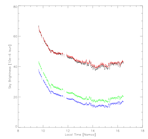
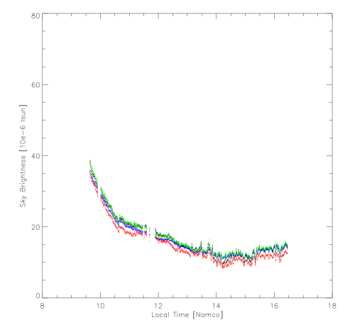
Figure 13: The variations of the sky brightness with the local time at Lake Namco before and after the calibration of the scattered light.

where $I_{sky}$ is the average intensity at the region several solar radii away from the solar disk and $I_{sun}$ is the true intensity at the solar disk center before weakened by the ND4 filter. We note that the scattered light of the SBM is not included in the above formula and the scattered light will be discussed in the next section. In our measurement, the region corresponding to $I_{sky}$ is between 5.0 to 7.0 solar radii excluding the projections of the supporting arms. For this purpose, we construct a mask based on the angular coordinates of the positions and the central coordinates of the ND4 filter. Then the mask is multiplied by the image of SBM. Next, we get rid of the region out of 7.0 solar radii and in 5.0 solar radii from the masked image according to the fitting position of the solar center and solar radius. The results are reported in Fig. 13.

The solar intensity $I_{sun}$ is usually computed in two ways: a central solar intensity is computed within $0.1R_{sun}$, or a mean solar intensity is computed using all pixels out to $1R_{sun}$ (Penn et al., 2004). Generally, the first way is adopted in former works (Penn et al., 2004; Lin and Penn, 2004; Liu et al., 2012b). However, the solar center in the image does not necessary coincide with the physical center of the Sun. This is mainly because the tube of SBM is not always perfectly parallel to the light ray during observations. The observers must adjust the position of the SBM after tracking the Sun for a period of time, which is about thirty minutes to two hours based on the desired alignment accuracy. Here we stress once again that the portability of the device is of great importance and we should avoid spending too much time with the alignment issue in a site survey. As a consequence, the mean solar intensity near the disk center may seem to ”sharply” change with time. In order to avoid this possible inconsistency, we adopt the intensity at the centroid of the solar disk in the image for the sky brightness calculations.

No.	Pass band	Sky brightness	Recording time (UT)	Zenith angle(∘)
0	Blue	35.7	2013-10-23T01:37:53	74.879
1	Green	39.1	2013-10-23T01:37:50	74.889
2	water	62.4	2013-10-23T01:37:55	74.872
3	Red	61.3	2013-10-23T01:37:45	74.905
4	Blue	37.8	2013-10-23T01:38:02	74.850
5	Green	42.4	2013-10-23T01:37:59	74.859
6	water	66.2	2013-10-23T01:38:04	74.843
7	Red	63.5	2013-10-23T01:37:57	74.866
…	…	…	…	…
…	…	…	…	…
5121	Blue	13.6	2013-10-23T07:08:30	45.859
5122	Green	16.9	2013-10-23T07:08:27	45.855
5123	water	38.8	2013-10-23T07:08:32	45.862
5124	Red	40.0	2013-10-23T07:08:25	45.852
5125	Blue	13.4	2013-10-23T07:08:39	45.873
5126	Green	17.0	2013-10-23T07:08:36	45.868
5127	water	38.7	2013-10-23T07:08:41	45.876
5128	Red	40.0	2013-10-23T07:08:34	45.865
…	…	…	…	…
…	…	…	…	…
10414	Blue	18.0	2013-10-23T04:30:26	47.058
10415	Green	22.1	2013-10-23T04:30:23	47.063
10416	water	44.4	2013-10-23T04:30:28	47.054
10417	Red	45.2	2013-10-23T04:30:21	47.066
10418	Blue	18.1	2013-10-23T04:30:35	47.042
10419	Green	21.8	2013-10-23T04:30:32	47.047
10420	water	45.0	2013-10-23T04:30:37	47.038
10421	Red	44.8	2013-10-23T04:30:30	47.051

Table 1: Sample results based on our automatic procedure on the raw data set taken on October 23, 2013 at Namco Lake in Tibet ($31^{\circ}$N, $90^{\circ}$E). The unit for sky brightness is in millionth of the corresponding solar disk center intensity.

4 Results and Analysis

In this part we highlight our analysis and approach; based on the techniques described in the previous sections; applied to the data set acquired on October 23, 2013 at Namco Lake in Tibet. Our procedure takes approximately four hours to automatically process the 10422 data with a normal PC with a dual-core processor (Intel Core i3-2350M CPU at 2.30GHz). The results are exported in a table-format output containing: the wave bands, recording time, sky brightness and solar zenith angle, respectively. These output results can subsequently be used for the evaluation of a series of important physical parameters. A short list sample of the results is reported in Table 1. Note that those raw data are not listed sequentially in time. Sorting the results by Julian date counts, due to the recording time, is an effective and necessary step for further calculations.

During the coronagraph site survey, the performance of the SBM instruments in long-time field work may cause unexpected parameter changes, such as increased scattered light levels for different wave bands. It is hence necessary to calibrate the scattered light levels frequently. According to Martinez-Pillet et al. (1990), the normalized sky brightness including a constant instrumental scattered light can be expressed as follows:

$$\frac{I_{sky}}{I_{sun}}=\phi_{\kappa}M+B,$$ (6)

where $\phi_{\kappa}$ is the atmospheric scattering function, $B$ is an instrumental constant which depends on wavelength and $M$ is the air mass. Following Lin and Penn (2004), the air mass column can be calculated as a function of zenith angle under the uniform curved atmospheric model:

$$M_{c}=-R\cos Z+\sqrt{R^{2}\cos^{2}Z+2Rt+t^{2}},$$ (7)

where $Z$ presents the zenith angle, $R$ equals the sum of the altitude and the radius of the Earth, and $t$ is the thickness of the atmosphere. Then we can get:

$$S(Z)=B-\alpha R\cos Z+\alpha\sqrt{R^{2}\cos^{2}Z+2Rt+t^{2}}$$ (8)

Therefore, we can fit the measured sky brightness $S(Z)$ as a function of $Z$ to the above formula, in which $B$, $\alpha$ and $t$ are three free parameters in the fitting algorithm.

Fig. LABEL:fig:14 displays the variations of the sky brightness measured with time in all four wavelengths throughout the course of a day. The fact that the measured sky brightness in the morning and in the afternoon, with the same zenith angles, can not overlap with each other, implies that the atmospheric conditions are not stable throughout the day. Lin and Penn (2004) did not suggest using this kind of data to fit the model. However, to obtain the fitted sky brightness we decide on adopting only the data during the morning time, i.e., the first half of the observations with better sky condition. The calibration parameters of the scattered light are 2.06, 5.13, 30.26 and 28.06 millionths for the blue, green, red and water vapor band-passes, respectively, obviously higher than those values reported in Liu et al. (2012b). The increased scattered-light levels indicate that the black coating material inside the SBM tube should have been seriously got faded after long-term sunshine exposed to high-energy radiation in high altitude environment. This problem will be resolved soon by coating the SBM tube regularly in the factory. The coefficients of the ND2 filters show little changes since we have tested them yearly. The variations of the sky brightness with the local time at Namco Lake before and after the calibration of the scattered light are shown in Fig. LABEL:fig:15.

Another possible application of our procedure is for guiding and tracking the Sun with high precision because our methodology can accurately derive the Sun’s center coordinates. Usually, a telescope can track an object using an extra guiding system composed by a tube parallel to the main telescope and an individual CCD imager. For field observation such as our site survey, the portable SBM instruments were not designed to be equipped with extra guiding system parallel to the main telescope tube. For most guiding systems for solar telescopes with full-disk observing mode, the Sun’s position for tracking is usually derived from the centroid of solar image. In one test with a white-light solar telescope of 100 mm aperture, we found the centroid of the Sun could deviate from that position, based on least-square fitting calculations, for about 50 pixels. In that test, the commercial CCD size is 5202 by 3454 pixels and the data are white-light full-disk solar images with solar diameter of about 3050 pixels. Moreover, our algorithm is more robust compared with the centroid method, because the fitting doesn’t require all the points of the Sun. When the Sun is partly covered by clouds, our algorithm can give the right results while the centroid method would not. Interestingly, all the solar telescopes with the full-disk mode can hence benefit from our algorithm and they can track the Sun without an extra guiding system.

5 Conclusions

For the solar site survey data analysis, we have developed one automatic procedure for the SBM instruments. A detailed description of the procedure is presented. The method can calculate the sky brightness, including identifying the solar disk and the sky areas around it as well as the excluded part of the supporting arms. These processes are implemented on our data acquired by different SBM instruments, including those made in China or lent from USA, during the site survey project in Western China. These results are significant and highly encouraging for further future efforts and investigations, particularly in deriving a variety of important physical parameters such as extinctions, aerosol content and precipitable water vapor content. Furthermore, the Sun’s accurate center coordinates derived in our procedure can be applied for tracking the Sun without an extra guiding system. Indeed, we are in a consulting phase with our engineers for a possible near-future practical realization of the project.

The preliminary analysis applying the results has been performed and discussed for the assessment of the levels of the scattered light. When we compare the scattered light levels obtained from this work with those taken 2 years ago (Liu et al., 2012b), we notice significant increase in every wavelength. This should be due to the functional degradation of the dark material coating inside the SBM tube which has been used after long-term sunshine exposure in the environment of the Tibet plateau. The new results about the scattered light levels will be reported after the tube is coated again in the near future. However, the robotization of our method for SBM data analysis has been tested and confirmed with high speed based on large data sample taken in the year of 2013 for various candidate sites, without any artificial intervention such as changing some parameters according to different SBM instruments or weather conditions as before.

Figure 4: An example of least-squares fitting. The dot-dashed line represents the algebraic fitting and the solid line represents the geometric fit.

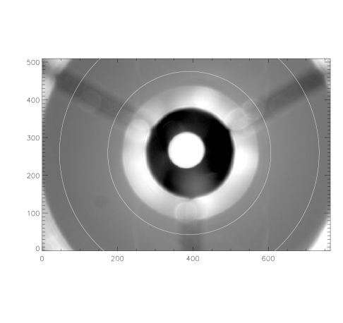
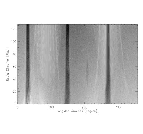
Figure 8: Taking the annular region from (a) and expanding it in polar coordinate.

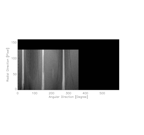
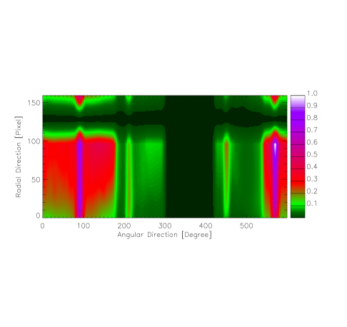
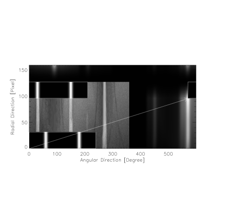
Figure 9: (a) is the padded edge image. (b) is the padded template. (c) is the cross-correlation between (a) and (b). (d) is the superimposed image of (a), (b) and(c).

Figure 12: Fitted sky brightness to the formula $S(Z)=B-\alpha R\cos Z+\alpha\sqrt{R^{2}\cos^{2}Z+2Rt+t^{2}}$ in four wavelengths. Blue, green, red and water vapor correspond to 450 nm, 530 nm, 890 nm and 940 nm, respectively.

References

- Evans (1948) Evans J. W., 1948, J. Opt. Soc. Am., 38, 1083
- Garcia and Yasukawa (1983) Garcia C. J., Yasukawa E. A., 1983, PASP. 95, 520
- Gander et al. (1994) Gander G., Golub G. H., Strebel R., 1994, BIT Numerical Mathematics, 34(4), 558
- Gonzalez and Woods (2002) Gonzalez R. C. and Woods R. E. , 2002, Digital Image Processing, 2nd edn. Prentice-Hall, Inc.
- Martinez-Pillet et al. (1990) Martinez-Pillet V., Ruis-Cobo B., Vazquez M., 1990, Sol. Phys., 125, 211
- Labonte (2003) Labonte B., 2003, Sol. Phys., 217, 367
- Lin and Penn (2004) Lin H., Penn M. J., Publ. Astron. Soc. Pac., 116, 652
- Liu et al. (2011) Liu N., Liu Y., Shen Y. D., Zhang X., Cao W., Jean A., 2011, Chinese Astron. Astroph., 35, 428
- Liu et al. (2012a) Liu S. Q., Duan J., Zhang X. F., Wen X., Qu Z. Q., Liu Y., 2012a, Astronomical Research and Technology, 9(2), 168 (in Chinese)
- Liu et al. (2012b) Liu Y., Shen Y. D., Zhang X. F., Liu N. P., 2012b, Sol. Phys., 279, 561
- Liu and Zhao (2013) Liu Y., Zhao L., 2013, MNRAS, 434, 1674
- Lyot (1930) Lyot B., 1930, CR. Acad. Sci. Paris., 191, 834
- Lyot (1939) Lyot B., 1939, MNRAS., 99, L580
- Otsu (1979) Otsu N., 1979, IEEE Trans. Sys. Man. Cyber., 9(1), 62
- Penn et al. (2004) Penn M. J., Lin H., Schmidt A., Gerke J., Hill F., 2004, Sol. Phys., 220, 107
- Wen et al. (2012) Wen X., Liu Y., Song T. F., Zhang X. F., Liu N. P., 2012, Astronomical Research and Technology, 9(2), 176 (in Chinese)