Quenching and anisotropy of hydromagnetic turbulent transport

Abstract

Hydromagnetic turbulence affects the evolution of large-scale magnetic fields through mean-field effects like turbulent diffusion and the $\alpha$ effect. For stronger fields, these effects are usually suppressed or quenched, and additional anisotropies are introduced. Using different variants of the test-field method, we determine the quenching of the turbulent transport coefficients for the forced Roberts flow, isotropically forced non-helical turbulence, and rotating thermal convection. We see significant quenching only when the mean magnetic field is larger than the equipartition value of the turbulence. Expressing the magnetic field in terms of the equipartition value of the quenched flows, we obtain for the quenching exponents of the turbulent magnetic diffusivity about 1.3, 1.1, and 1.3 for Roberts flow, forced turbulence, and convection, respectively. However, when the magnetic field is expressed in terms of the equipartition value of the unquenched flows these quenching exponents become about 4, 1.5, and 2.3, respectively. For the $\alpha$ effect, the exponent is about 1.3 for the Roberts flow and 2 for convection in the first case, but 4 and 3, respectively, in the second. In convection, the quenching of turbulent pumping follows the same power law as turbulent diffusion, while for the coefficient describing the $\bm{\varOmega}\times\bm{{J}}$ effect nearly the same quenching exponent is obtained as for $\alpha$. For forced turbulence, turbulent diffusion proportional to the second derivative along the mean magnetic field is quenched much less, especially for larger values of the magnetic Reynolds number. However, we find that in corresponding axisymmetric mean-field dynamos with dominant toroidal field the quenched diffusion coefficients are the same for the poloidal and toroidal field constituents.

1. Introduction

Many astrophysical objects possess turbulent convection, and the dynamo mechanisms based on it are believed to be responsible for the generation and maintenance of the observed magnetic fields. The study of the dynamo mechanism in the solar convection zone using simulations of turbulent convection in spherical shells began in the 1980s with the works of GM81, Gil83 and Gla85, and has recently been pursued further by many more authors (brun04; racine11; K12; K13; KKKB14). However, under stellar conditions the dimensionless parameters governing magnetohydrodynamics attain extreme values, which are far from being accessible through numerical models. So we do not know to what extent feasible models at temperate parameter regimes reflect properties of convection and dynamos in real stars. An alternative approach to studying the dynamo problem is mean-field theory which began with the pioneering works of Par55, Bra64, and SKR66. This approach is computationally less expensive because one needs not to resolve the full dynamical range of the small-scale turbulence, which is instead parameterized. In recent years, there have been significant achievements of mean-field MHD in reproducing various aspects of magnetic and flow fields in the Sun (e.g., CNC04; rempel06; KKT06; CK09; CK12; Ka10; char10; PK11).

In this context, an important task is to determine the mean electromotive force $\overline{\mbox{\boldmath${\mathcal{E}}$}}{}$, which results from the correlation between the fluctuating constituents of velocity and magnetic field, in terms of the mean field $\bm{\overline{{B}}}$. There is no accurate theory to accomplish this task from first principles, except for some limiting cases, in particular those of small Strouhal and magnetic Reynolds number, $R_{\mathrm{m}}$. Therefore, suitable assumptions are required in determining $\overline{\mbox{\boldmath${\mathcal{E}}$}}{}$. When $\bm{\overline{{B}}}$ varies slowly in space and time, we may write

$$\overline{\cal E}{}_{i}=\alpha_{ij}\overline{B}_{j}+\beta_{ijk}\frac{\partial\overline{B}_{j}}{\partial x_{k}}.$$ (1)

The diagonal components of $\alpha_{ij}$ are usually the most important terms for dynamo action, but in the presence of shear, the $\bm{\varOmega}\times\bm{{J}}$ (KR80) and shear-current (RK03) effects, both covered by $\beta_{ijk}$, can also enable it. Many components of $\beta_{ijk}$, however, describe dissipative effects.

Doubts can be raised regarding the explanatory and predictive power of mean-field dynamo models given that the tensors $\alpha_{ij}$ and $\beta_{ijk}$ are often chosen to some extent arbitrarily or even tuned to obtain results resembling features of the Sun. Therefore, methods to measure these coefficients from simulations have been developed. At present the most accurate method is the so-called test-field method (Sch05; Sch07; BRRS08; BGKKMR13). In this method, one selects an adequate number of independent mean fields, the ‘test fields’, and solves for each of them the corresponding equation for the fluctuating magnetic field (in addition to the main simulation). Finally, via computing the mean electromotive force, the transport coefficients are calculated.

There are different variants of the test-field method. The best established one is based on the average over two spatial (the ‘horizontal’) coordinates. This method has been applied to a large variety of setups, e.g., isotropic homogeneous turbulence (SBS08; BRRS08), homogeneous shear flow turbulence (BRRK08), with and without helicity (MKTB09), turbulent convection (KKB09a), and supernova driven interstellar turbulence (G13). Another variant is based on Fourier-weighted horizontal averages and allows to determine also the coefficients that multiply horizontal derivatives of the mean field. This method has been applied to forced turbulence (BRK12) and to cosmic ray-driven turbulence (RKBE12; BBMO13).

In models based on thin flux tubes, forming the major alternative to distributed turbulent dynamos, the magnetic field strength in the deep parts of the solar convection zone is believed to exceed its value at equipartition with velocity (CG87; DC93; WFM11). On the other hand, it is well known that turbulent transport becomes less efficient when the mean magnetic field’s strength is comparable to or larger than the equipartition value. Therefore precise knowledge of the quenching is needed. Mean-field dynamo models of the $\alpha\varOmega$ type often employ an ‘ad hoc’ algebraic or dynamical $\alpha$-quenching (Jep75; covas98), while largely ignoring the quenching of the turbulent diffusivity $\eta_{\rm t}$ despite of its importance in determining the cycle frequency. Indeed, in the absence of quenching, the standard estimate of $\eta_{\rm t}$ for the Sun ($\sim 10^{12}$–$10^{13}\,{\rm cm}^{2}\,{\rm s}^{-1}$) yields a rather short cycle period of $2$–$3\,{\rm yr}$ (Koh73). However, by considering the quenching of $\eta_{\rm t}$, a reasonable value of the cycle period can easily be obtained (R94; GDD09; MNM11). In fact, measuring the cycle frequency in a simulation has been one way of determining the quenching of $\eta_{\rm t}$ (KB09).

Early work by Mof72 and Rue74 showed that under the Second Order Correlation Approximation (SOCA), $\alpha$ is quenched inversely proportional to the third power of the magnetic field. Following VC92, several investigations have suggested that $\alpha$ is beginning to be quenched noticeably when the mean field becomes comparable to $R_{\mathrm{m}}^{-1}$ times the equipartition value (CH96), i.e., for extremely weak magnetic fields. This behavior is also called ‘catastrophic quenching’. However, it is now understood as an artifact of having defined volume-averaged mean fields (B01; BRRS08) combined with the usage of perfectly conducting or periodic boundary conditions and is not expected to be important in astrophysical bodies where magnetic helicity fluxes can alleviate catastrophic quenching (e.g., KMRS00; DSGB13). The actual value of $\alpha$ shows a much weaker dependence on $R_{\mathrm{m}}$ even when $\overline{B}$ is comparable with the equipartition value (BRRS08). This work also shows that the $R_{\mathrm{m}}$ dependence of $\alpha$ and $\eta_{\rm t}$ is such that their contributions to the growth rate nearly balance, with a residual matching the microscopic resistive term. This is in fact a requirement for the dynamo to be in a saturated state. Consequently the saturated mean electromotive force is proportional to $R_{\mathrm{m}}^{-1}$, which is sometimes misinterpreted as catastrophic quenching.

Once catastrophic quenching is alleviated, the magnetic field can grow to equipartition field strengths, when other quenching mechanisms that are not $R_{\mathrm{m}}$ dependent might become important and can therefore be studied already for smaller values of $R_{\mathrm{m}}$. SBS07 found that $\alpha$ is quenched proportional to $1/\overline{B}^{2}$ and $1/\overline{B}^{3}$ for time-dependent and steady flows, respectively. Their latter result was based on analytic theory and appeared to be confirmed by numerical simulations using a steady forcing proportional to the ABC-flow. However, subsequent work by RB10 demonstrated quenching proportional to $\overline{B}^{\,-4}$ for a steady forcing proportional to the flow I of Rob72, hereafter referred to as Roberts flow. They also noted that for ABC-flow forcing the quenching is indeed better described when setting the power also to 4 instead of 3. More recently, in supernova driven turbulent dynamo simulations, G13 find $\alpha\sim(\overline{B}/B_{\rm eq})^{-2}$ where $B_{\rm eq}$ is the local equipartition value.

For the turbulent diffusivity, KPR94 and RK00 obtained that $\eta_{\rm t}$ is quenched inversely proportional to $\overline{B}$. In the two-dimensional case, CV91 have found catastrophic quenching of $\eta_{\rm t}$. However, this is a special situation connected with the fact that in two dimensions the mean square vector potential is a conserved quantity. This is no longer the case in three dimensions. Quenching similar to KPR94 has been confirmed by simulations (B01; BB02; G13). In particular, making the ansatz $\eta_{\rm t}\sim 1/\big{(}1+p(\overline{B}/B_{\rm eq})^{q}\big{)}$, G13 find $q\approx 1$ in supernova-driven simulations of the turbulent interstellar medium. On the other hand, YBR03 find $q\approx 2$ in simulations of forced turbulence with a decaying large-scale magnetic field. However KB09 found that their results depend on the strength of shear and found $q\approx 1$ for weak shear while $q\approx 2$ for strong shear.

In the present work we measure the quenching of these transport coefficients as a function of the mean magnetic field strength for three different background simulations – (i) a forced Roberts flow, (ii) forced turbulence in a triply periodic box, and (iii) convection in a bounded box. In all these simulations we impose a uniform and constant external mean field. However, this induces a preferred direction which causes the statistical properties of the turbulence to be axisymmetric with respect to the direction of the magnetic field. In the following, we refer to such flows as axisymmetric turbulence, for which the number of independent components of the $\alpha$ and $\eta$ tensors is reduced to only nine, simplifying also their determination (BRK12).

2. Concept of turbulent transport in mean-field dynamo

The evolution of the magnetic field $\bm{{B}}$ in an electrically conducting fluid is governed by the induction equation

$${\partial\bm{{B}}\over\partial t}=\mbox{\boldmath$\nabla$}{}\times\left(\bm{{U}}\times\bm{{B}}-\eta\bm{{J}}\right),$$ (2)

where $\bm{{U}}$ is the fluid velocity. Here, $\eta$ is the microphysical magnetic diffusivity, while the magnetic permeability of the fluid has been set to unity. Thus the current density $\bm{{J}}$ is given by $\bm{{J}}=\mbox{\boldmath$\nabla$}{}\times\bm{{B}}$. In mean-field MHD, we consider the fields as sums of ‘averaged’ and small-scale ‘fluctuating’ fields, with the assumption that the averaging satisfies (at least approximately) the Reynolds rules. Denoting averaged fields by overbars and fluctuating ones by lowercase letters, we write the equation for the mean magnetic field $\bm{\overline{{B}}}$ as

$${\partial\bm{\overline{{B}}}\over\partial t}=\mbox{\boldmath$\nabla$}{}\times\left(\bm{\overline{{U}}}\times\bm{\overline{{B}}}+\overline{\mbox{\boldmath${\mathcal{E}}$}}{}-\eta\bm{\overline{{J}}}\right),$$ (3)

where $\overline{\mbox{\boldmath${\mathcal{E}}$}}{}=\overline{\bm{{{u}}}\times\bm{{{b}}}}$ is the aforementioned mean electromotive force, which captures the correlation of the fluctuating fields $\bm{{{u}}}$ and $\bm{{{b}}}$. The ultimate goal of mean-field MHD is to express $\overline{\mbox{\boldmath${\mathcal{E}}$}}{}$ in terms of $\bm{\overline{{B}}}$ itself. There are several procedures for doing that. When the mean magnetic field varies slowly in space and time we can write $\overline{\mbox{\boldmath${\mathcal{E}}$}}{}$ in the form of Equation (1). Our primary goal is to measure the transport coefficients $\alpha_{ij}$ and $\eta_{ijk}$ in the presence of an imposed uniform magnetic field $\bm{{B}}_{\rm ext}$ and, in particular, measure the degree of their quenching and anisotropy.

Let us consider turbulence that is anisotropic and exhibiting only one preferred direction $\hat{\mbox{\boldmath$e$}}{}$, referring to an external magnetic field, rotation axis, or the direction of gravity. Then following BRK12, the general representation of $\overline{\mbox{\boldmath${\mathcal{E}}$}}{}$ is given by

$$\overline{\mbox{\boldmath${\mathcal{E}}$}}{}=\phantom{-} \alpha_{\perp}\bm{\overline{{B}}} +(\alpha_{\parallel}-\alpha_{\perp}) (\hat{\mbox{\boldmath$e$}}{}\cdot\bm{\overline{{B}}}) \hat{\mbox{\boldmath$e$}}{} +\gamma\hat{\mbox{\boldmath$e$}}{}\times\bm{\overline{{B}}}$$

$$- \eta_{\perp}\bm{\overline{{J}}} -(\eta_{\parallel}-\eta_{\perp}) (\hat{\mbox{\boldmath$e$}}{}\cdot\bm{\overline{{J}}}) \hat{\mbox{\boldmath$e$}}{} -\delta\hat{\mbox{\boldmath$e$}}{}\times\bm{\overline{{J}}}$$ (4)

$$- \kappa_{\perp}\bm{\overline{{K}}} -(\kappa_{\parallel}-\kappa_{\perp}) (\hat{\mbox{\boldmath$e$}}{}\cdot\bm{\overline{{K}}}) \hat{\mbox{\boldmath$e$}}{} -\mu\hat{\mbox{\boldmath$e$}}{}\times\bm{\overline{{K}}}$$

with nine coefficients $\alpha_{\perp}$, $\alpha_{\parallel}$, $\ldots$, $\mu$. While $\bm{\overline{{J}}}$ is given by the antisymmetric part of the gradient tensor $\mbox{\boldmath$\nabla$}{}\bm{\overline{{B}}}$, $\bm{\overline{{K}}}$ is defined by $\bm{\overline{{K}}}=\hat{\mbox{\boldmath$e$}}{}\cdot(\mbox{\boldmath$\nabla$}{}\bm{\overline{{B}}})^{\mathrm{S}}$ with $(\mbox{\boldmath$\nabla$}{}\bm{\overline{{B}}})^{\mathrm{S}}$ being the symmetric part of $\mbox{\boldmath$\nabla$}{}\bm{\overline{{B}}}$. For homogeneous isotropic turbulence $\alpha_{\parallel}=\alpha_{\perp}$, $\eta_{\parallel}=\eta_{\perp}$ and the other coefficients vanish. We note that our sign convention for $\alpha_{\perp}$, $\alpha_{\parallel}$, and $\gamma$ follows that commonly used, but it differs from that used in BRK12.

The $\mu$ term corresponds to a modification of turbulent diffusion along the preferred direction. To understand this, let us assume that only $\eta_{\perp}$, $\eta_{\|}$, and $\mu$ are non-vanishing and independent of position. By introducing the quantities $\eta_{\rm T}\equiv\eta_{\rm t}+\eta$ with $\eta_{\rm t}\equiv\eta_{\perp}-\mu/2$ and $\epsilon\equiv\eta_{\parallel}-\eta_{\perp}+\mu/2$, we have

$${\partial\bm{\overline{{B}}}\over\partial t}=\eta_{\rm T}\mbox{\boldmath$\nabla$}{}^{2}\bm{\overline{{B}}}+\mu\nabla^{2}_{\|}\bm{\overline{{B}}}+\epsilon\left(\mbox{\boldmath$\nabla$}{}_{\perp}^{2}\bm{{B}}_{\perp}+\mbox{\boldmath$\nabla$}{}_{\perp}\nabla_{\|}B_{\|}\right),$$ (5)

which shows that positive values of $\mu$ correspond to an enhancement of turbulent diffusion along the preferred direction. As Equation (5) reveals, $\eta_{\|}$ and $\eta_{\perp}$ do not characterize the diffusion parallel and perpendicular to the preferred direction, as their symbols might suggest.

An anisotropy similar to that of Equation (5) has been considered in connection with the turbulent decay of sunspot magnetic fields (RK00b), where the mean magnetic field defines the preferred direction. It has not yet been used in mean-field dynamo models, where, however, anisotropies of the turbulent diffusivity due to the simultaneous influence of rotation and stratification have been taken into account (RB95; PK14) .

3. The Model Setup

We distinguish two basically different schemes of establishing the background flow: by a prescribed forcing or by the convective instability. In the first case, both laminar and turbulent (artificially forced) flows will be considered. With respect to the fluid, we generally think of an ideal gas with state variables density $\rho$, pressure $p$ and temperature $T$, adopting, however, different effective equations of state for the two schemes.

The continuity and induction equations are shared by both schemes and take the form

$${D\ln\rho\over Dt} =-\mbox{\boldmath$\nabla$}{}\cdot\bm{{U}},$$ (6)

$${\partial\bm{{A}}\over\partial t} =\bm{{U}}\times\bm{{B}}+\eta\mbox{\boldmath$\nabla$}{}^{2}\bm{{A}}\,.$$ (7)

Here $D/Dt=\partial/\partial t+\bm{{U}}\cdot\bm{\mbox{\boldmath$\nabla$}{}}$ is the advective time derivative and $\bm{{A}}$ is the magnetic vector potential. The magnetic field includes the imposed field, i.e., ${\bm{{B}}}={\bm{{B}}}_{\rm ext}+\mbox{\boldmath$\nabla$}{}\times{\bm{{A}}}$, and the microscopic diffusivity $\eta$ is constant.

3.1. Forced flows

In these models, we assume the fluid to be isothermal, which implies for its equation of state $p=c_{\rm s}^{2}\rho$, with the constant sound speed $c_{\rm s}$. Hence we solve equations (6) and (7) together with the momentum equation,

$${D\bm{{U}}\over Dt} =-c_{\rm s}^{2}\mbox{\boldmath$\nabla$}{}\ln\rho+\rho^{-1}(\bm{{J}}\times\bm{{B}}+\mbox{\boldmath$\nabla$}{}\!\cdot\!2\rho\nu\mbox{\boldmath${\sf S}$}{})+\bm{{{f}}}.$$ (8)

Here $\nu={\rm const}$ is the kinematic viscosity, and $\bm{{{f}}}$ is a forcing function to be specified below. The traceless rate of strain tensor ${\sf S}$ is given by

$${\sf S}_{ij}={\textstyle{1\over 2}}(U_{i,j}+U_{j,i})-{\textstyle{1\over 3}}\delta_{ij}\bm{\nabla}\cdot\bm{U},$$ (9)

where the commas denote partial differentiation with respect to the coordinate $j$.

The simulation domain for this model is periodic in all directions with dimension $L_{x}\times L_{x}\times L_{z}$, that is, horizontally isotropic. In the following we always use $L_{x}=L_{y}\equiv L$ and express lengths in units of the inverse of the wavenumber $k_{1}=2\pi/L$.

3.1.1 Roberts forcing

First we use a laminar forcing to maintain one of the flows for which Rob72 had demonstrated dynamo action, namely his flow I. It is incompressible, independent of $z$, and all 2nd-rank tensors obtained from it by $xy$ averaging are symmetric about the $z$ axis (Rae02a). The flow is defined by

$$\bm{{{u}}}_{0}=-\hat{\mbox{\boldmath$z$}}{}\times\mbox{\boldmath$\nabla$}{}\psi+k_{\rm f}\psi\hat{\mbox{\boldmath$z$}}{}\,,$$ (10)

where

$$\psi=(u_{0}/k_{0})\cos k_{0}x\,\cos k_{0}y\,,\quad k_{\rm f}=\sqrt{2}\,k_{0}\,,$$ (11)

with constant $u_{0}$ and $k_{0}$. Note that this flow is maximally helical, i.e. $\mbox{\boldmath$\nabla$}{}\times\bm{{{u}}}_{0}=k_{\rm f}\bm{{{u}}}_{0}$. We define the forcing $\bm{{{f}}}$ such that for $\bm{{B}}=\bm{0}$, the flow (10) with $\rho=\rho_{0}={\rm const}$ is an exact solution of Equation (8):

$$\bm{{{f}}}=\nu k_{0}^{2}\bm{{{u}}}_{0}+\bm{{{u}}}_{0}\cdot\mbox{\boldmath$\nabla$}{}\bm{{{u}}}_{0}\;\;\left(=\nu k_{0}^{2}\bm{{{u}}}_{0}+{\textstyle{1\over 2}}\mbox{\boldmath$\nabla$}{}\bm{{{u}}}_{0}^{2}\right).$$ (12)

We perform several simulations with different strengths of the external magnetic field $\bm{B}_{\rm ext}$ with this flow.

3.1.2 Forced turbulence

Here we employ for $\bm{{{f}}}$ a random forcing function, namely a linearly polarized wave with wavevector and phase being changed randomly between integration timesteps (B01). The driven flow is non-helical and known to lack an $\alpha$ effect (BRRK08). The averaged modulus of the wavevector is denoted by $k_{\rm f}$ and the ratio $k_{\rm f}/k_{1}$ is referred to as the scale separation ratio. To achieve sufficiently large scale separation, we would need to keep $k_{\mathrm{f}}/k_{1}$ large. However, in this case $R_{\mathrm{m}}=u_{\rm rms}/\eta k_{\mathrm{f}}$ becomes small. Therefore we use $k_{\mathrm{f}}/k_{1}\geq 5$ as a compromise.

3.2. Convection

In this model the background flow is generated by convection and consequently we employ $p=(c_{p}-c_{v})\rho T$ for the equation of state of the fluid, where $c_{p}$ and $c_{v}$ are the specific heats at constant pressure and volume, respectively. Our model is similar to many earlier studies in the literature (e.g., BJNRST96; OSB01; KKB08; KKB09a; KKB09b). Its computational domain is a rectangular box consisting of three layers: the lower part ($-0.85<z/d<0$) is a convectively stable overshoot layer, the middle part ($0\leq z/d\leq 1$) is convectively unstable, and the upper part ($1<z/d<1.15$) is an almost isothermal cooling layer. The overshoot layer was made comparatively thick to guarantee that the overshooting is not affected by the lower boundary. The box dimensions are $(L_{x},L_{y},L_{z})=(5,5,2)d$, where $d$ is the depth of the unstable layer. Gravity is acting in the downward direction (i.e., along the negative $z$-direction). By including rotation about the $z$ axis, we can consider the simulation box as a small portion of a star located at one of its poles. The mass conservation and induction equations (6), (7) are now complemented by a modified momentum equation and an equation for the internal energy per unit mass (BJNRST96)

$$\frac{D\bm{U}}{Dt} =-\frac{\bm{\mbox{\boldmath$\nabla$}{}}p}{\rho}+{\bm{g}}-2\bm{\varOmega}\times\bm{U}+\frac{1}{\rho}(\bm{{J}}\times\bm{{B}}+\bm{\mbox{\boldmath$\nabla$}{}}\cdot 2\nu\rho\mbox{\boldmath${\sf S}$}),$$

$$\frac{De}{Dt} =-\frac{p}{\rho}\bm{\mbox{\boldmath$\nabla$}{}}\!\cdot\bm{{U}}+\frac{1}{\rho c_{v}}\bm{\mbox{\boldmath$\nabla$}{}}\!\cdot\!K(z)\bm{\mbox{\boldmath$\nabla$}{}}e+2\nu\mbox{\boldmath${\sf S}$}^{2}+\frac{\eta\mu_{0}}{\rho}\bm{{J}}^{2}-\frac{e\!-\!e_{0}}{\tau(z)}.$$ (13)

Here, $\bm{g}=-g\hat{\bm{z}}$, with $g>0$, is the gravitational acceleration, $\bm{\varOmega}=\varOmega_{0}(-\sin\theta,0,\cos\theta)$ is the rotation vector with $\theta$ its angle against the $z$ direction, and $K$ is the heat conductivity with a piecewise constant $z$ profile to be specified below. The specific internal energy is related to the temperature via $e=c_{v}T$. In the energy equation (13), the last term is of relaxation type and regulates the internal energy to settle on average close to $e_{0}={\rm const}$. As there is permanent heat input from the lower boundary and from viscous heating, it effectively acts as a cooling. The relaxation rate $\tau(z)^{-1}$ has a value of $75\sqrt{g/d}$ within the cooling layer and drops smoothly to zero within the unstable layer over a transition zone of width $0.025d$.

The vertical boundary conditions for the velocity are chosen to be impenetrable and stress free, i.e.,

$$U_{x,z}=U_{y,z}=U_{z}=0,$$ (14)

while for the magnetic field we use the vertical field boundary condition $B_{x}=B_{y}=0$. A steady influx of heat $F_{0}=-(K\partial_{z}e)(x,y,-0.85d)/c_{v}$ at the bottom of the box and a constant temperature, i.e., constant internal energy, at its top is maintained, where the latter is specified to be just equal to $e_{0}$ occurring in the relaxation term. The $x$ and $y$ directions are periodic for all fields.

The input parameters are now determined in the following somewhat indirect way: Instead of prescribing $K$, it is assumed that the hydrostatic reference solution coincides in the overshoot and unstable layers with a polytrope, the index $m$ of which is prescribed. Here we choose $m=3$ and $m=1$, respectively. As for a polytrope $de/dz=-g/(m+1)(\gamma-1)$, $\gamma=c_{p}/c_{v}$, and at each $z$ we have $F_{0}=-(K/c_{v})de/dz={\rm const}$, the heat conductivity is obtained as $K=c_{v}(m+1)(\gamma-1)F_{0}/g$, i.e., it is also piecewise linear (for a physical motivation, see HTM86). For simplicity it is assumed that in the cooling layer, for which no polytrope exists, $K$ has the same value as in the unstable one. Within the ranges of the other control parameters covered by our simulations, it is then guaranteed that the relaxation to the quasi-isothermal state is dominated by the term $-e/\tau$.

The convection problem is governed by a set of dimensionless control parameters comprising the Prandtl, Taylor, and Rayleigh numbers

Pr $$=\frac{\nu}{\chi(z_{\rm m})},\ \ \mbox{\rm Ta}=\frac{4\varOmega^{2}d^{4}}{\nu^{2}},$$ (15)

Ra $$=\frac{gd^{4}}{\nu\chi(z_{\rm m})H_{p}(z_{\rm m})}\Delta\nabla(z_{\rm m}),$$ (16)

along with the dimensionless pressure scale height at the top

$$\xi_{0}=(\gamma-1)e_{0}/gd.$$ (17)

For the calculation of the Prandtl and Rayleigh numbers, the values of the thermal diffusivity $\chi=K/\rho c_{p}$, the superadiabatic gradient $\Delta\nabla={\rm d}(s/c_{\rm P})/{\rm d}\ln p$ and the pressure scale height $H_{p}$ of the associated hydrostatic equilibrium solution are taken from the middle of the convective layer at $z_{\rm m}=d/2$. The density contrast within the unstable layer is

$${\rho(0)\over\rho(d)}=1+{gd\over 2(\gamma-1)e_{0}}=1+{1\over 2\xi_{0}}.$$ (18)

Hence, the parameter $\xi_{0}$ controls the density stratification in our domain. We use $\xi_{0}=3/25$ in all the simulations which results in a (hydrostatic) density contrast of $31/6$; $\gamma$ was fixed to $5/3$ throughout and the different models have the same initial density at $z=z_{\rm m}$.

Equation (18) assumes that $e=e_{0}$ at the top of the convective layer, which cannot be exactly true. In the simulations this error is increased by the fact that the effect of the cooling reaches somewhat below $z/d=1$. This leads to a higher density contrast ($\approx 8$) in the actual hydrostatic solution.

3.3. Diagnostics

As diagnostics we use the fluid and magnetic Reynolds numbers as well as the Coriolis number

$$\mbox{\rm Re}=\frac{u_{\rm rms}}{\nu k_{\mathrm{f}}},\quad R_{\mathrm{m}}=\frac{u_{\rm rms}}{\eta k_{\mathrm{f}}},$$ (19)

where for the convection setup $k_{\mathrm{f}}=2\pi/d$ is an estimate of the wavenumber of the largest energy-carrying eddies. $u_{\rm rms}=\langle\bm{{{u}}}^{2}\rangle^{1/2}$ is the rms value of the velocity with $\langle\cdot\rangle$ denoting the average over the whole box or, for the convection setup, over the unstable layer only, i.e. $0\leq z/d\leq 1$. The values for $B_{\rm ext}=0$, i.e., for the unquenched state, are marked by the subscript 0. When we quote these values for a set of runs with different field strengths, they apply to the case with weakest field, i.e., the unquenched state. However for $R_{\mathrm{m}}$ we quote both the unquenched value, denoted by $R_{\mathrm{m0}}$, and the quenched value for the run with the strongest field strength.

All simulations are performed using the Pencil Code, which uses sixth-order finite differences in space and a third order accurate explicit time stepping method.

3.4. Test-field methods

The goal of the test-field method is to measure the turbulent transport coefficients completely from given flow fields $\bm{{U}}$, which can either be prescribed explicitly or produced by a numerical simulation, called the main run. To accomplish this, the equation for the fluctuating fields

$${\partial\mbox{\boldmath$a$}{}^{T}\over\partial t}=\bm{\overline{{U}}}\times\bm{{{b}}}^{T}+\bm{{{u}}}\times\bm{\overline{{B}}}^{T}+(\bm{{{u}}}\times\bm{{{b}}}^{T})^{\prime}+\eta\mbox{\boldmath$\nabla$}{}^{2}\mbox{\boldmath$a$}{}^{T}$$ (20)

is solved for a set of prescribed test fields $\bm{\overline{{B}}}^{T}\!\!$. Here $\bm{{{b}}}^{T}=\mbox{\boldmath$\nabla$}{}\times\mbox{\boldmath$a$}{}^{T}$ and the prime denotes the operation of extracting the fluctuation of a quantity. Each $\mbox{\boldmath$a$}{}^{T}$ results in a mean electromotive force

$$\overline{\mbox{\boldmath${\mathcal{E}}$}}{}{\,}^{T}=\overline{\bm{{{u}}}\times\bm{{{b}}}^{T}},$$ (21)

and if the test fields are independent and their number is adjusted to that of the desired components in $\alpha_{ij}$ and $\beta_{ijk}$, the system (21) can be inverted unambiguously. For the truncated ansatz (1), test fields which depend linearly on position are suitable. However, when truncation is to be overcome, Equation (1) can be considered as the Fourier space representation of the most general $\overline{\mbox{\boldmath${\mathcal{E}}$}}{}$–$\bm{\overline{{B}}}$ relationship. Then $\alpha_{ij}$ and $\beta_{ijk}$ are functions of wavevector $\bm{{{k}}}$ and angular frequency $\omega$ of the Fourier transform and it is natural to specify the test fields to be harmonic in space (BRS08) and time (HB09). By varying their $\bm{{{k}}}$ and $\omega$, arbitrarily close approximations to the general $\overline{\mbox{\boldmath${\mathcal{E}}$}}{}$–$\bm{\overline{{B}}}$ relationship can be obtained (see, e.g., Rae14).

3.4.1 Test-field method for horizontal ($z$-dependent) averages

We will employ two different flavors of the test-field method. For the first one we define mean quantities by averaging over all $x$ and $y$. Then, necessarily, $\overline{B}_{z}={\rm const}$ and for homogeneous turbulence it is sufficient to consider horizontal mean fields $\bm{\overline{{B}}}=\left(\overline{B}_{x}(z,t),\overline{B}_{y}(z,t),0\right)$ only. When restricting ourselves to the limit of stationarity, our $\bm{{{k}}}$ dependent test fields have the following form:

$$\overline{\bm{B}}^{1\rm c} = B_{0}(\cos kz,0,0),\;\;\;\overline{\bm{B}}^{2\rm c}=B_{0}(0,\cos kz,0),\quad$$

$$\overline{\bm{B}}^{1\rm s} = B_{0}(\sin kz,0,0),\quad\overline{\bm{B}}^{2\rm s}=B_{0}(0,\sin kz,0),$$ (22)

where $k=k_{z}$ and in most of the simulations we use $k=k_{1}$. The $z$ component of $\overline{\mbox{\boldmath${\mathcal{E}}$}}{}$ does not influence $\bm{\overline{{B}}}$, thus only its $x$ and $y$ components matter and we have

$$\overline{\cal E}{}_{i}=\alpha_{ij}\overline{B}_{j}-\eta_{ij}\overline{J}_{j},$$ (23)

with $i,j=1,2$ and $\eta_{i1}=\beta_{i23}$ and $\eta_{i2}=-\beta_{i13}$. That is, we can derive eight coefficients (four $\alpha$ and four $\eta$) using the above test fields. Our main interest is to compute the diagonal components of $\alpha_{ij}$ and $\eta_{ij}$. However, in some cases we also study the off-diagonal components. Since the resulting turbulent transport coefficients depend only on $z$ (in addition to $t$), we call this variant of the test-field method TFZ. It is implemented in the Pencil Code and discussed in detail by BRRS08.

It is convenient to discuss the results in terms of the quantities

$$\alpha = {\textstyle{1\over 2}}(\alpha_{11}\!+\!\alpha_{22}),\;\;\gamma ={\textstyle{1\over 2}}(\alpha_{21}\!-\!\alpha_{12}),$$ (24)

$$\eta_{\rm t} = {\textstyle{1\over 2}}(\eta_{11}\!+\!\eta_{22}),\;\;\delta ={\textstyle{1\over 2}}(\eta_{21}\!-\!\eta_{12}),$$

which cover an important subset of all the eight coefficients.

3.4.2 Test-field method for axisymmetric turbulence

Next, we turn to another variant of the test-field method that allows us to calculate all nine coefficients in Equation (4) under the restriction of axisymmetric turbulence. It is then necessary to consider mean fields that depend on more than one dimension, as otherwise the gradient tensor $\mbox{\boldmath$\nabla$}{}\bm{\overline{{B}}}$ can be expressed completely by the components of $\bm{{J}}$ and the coefficients $\kappa_{\perp}$, $\kappa_{\parallel}$ and $\mu$ cannot be separated from $\eta_{\perp}$, $\eta_{\parallel}$ and $\delta$. Hence we now admit mean fields depending on all three spatial coordinates and define the mean by spectral filtering. We specify it such that only field constituents whose components $\sim\sum_{j}c_{j}(z)\exp{\rm i}\overline{\bm{{{k}}}}_{j}\cdot\bm{{{x}}}_{\perp}$ contribute to the mean. Here $\bm{{{x}}}_{\perp}=(x,y)$ is the position vector in horizontal planes and the sum is over all two-dimensional wavevectors $\overline{\bm{{{k}}}}_{j}$ of the form $(\pm\overline{k}_{x},\pm\overline{k}_{y})$ with fixed $\overline{k}_{x},\overline{k}_{y}>0$. So averaging means here to perform the operation

$$\hskip 2.84526pt\overline{f}(x,y,z)=\frac{1}{A}\sum_{j}\!\!\int_{A}f(x^{\prime},y^{\prime},z){\rm e}^{{\rm i}\overline{\bm{{{k}}}}_{j}\cdot(\bm{{{x}}}_{\perp}-\bm{{{x}}}_{\perp}^{\prime})}dx^{\prime}dy^{\prime},$$ (25)

where $A$ is the horizontal cross-section of the box. We call this variant of the test-field method for axisymmetric turbulence TFA and refer for further details to BRK12. In our case, the preferred direction is given by that of the externally imposed magnetic field.

As we will apply this method only with horizontally isotropic periodic boxes with $L_{x}=L_{y}=L$, we may choose $\overline{k}_{x}=\overline{k}_{y}=k_{1}=2\pi/L$. In general, it makes not much sense to choose $\overline{k}_{x}$ or $\overline{k}_{y}$ different from these smallest possible values for the corresponding extents of a given box. Otherwise, possible field constituents with smaller wavenumbers would be counted to the ‘fluctuations’ which is hardly desirable. Even for our choice $\overline{k}_{x},\overline{k}_{y}=k_{1}$ this could be a problem, namely with respect to constituents with horizontal wavenumber $k_{x}$ or $k_{y}$ equal to zero, so their occurrence should be avoided. As we apply TFA only to homogeneous turbulence (fully periodic boxes), this is granted.

Spectral filtering, being clearly useful for comparisons with observations, is known to violate in general the Reynolds rule $\overline{\overline{F}g}=0$. However, if in the $\bm{{{k}}}$ spectrum of the quantity $G=\overline{G}+g$ there are “gaps” at $k_{x},k_{y}=2k_{1}$ (for our choice) with vanishing spectral amplitudes, this rule is granted. Such gaps, albeit only in the form of amplitude depressions, can emerge in the saturated stage of a turbulent dynamo; see B01 for examples, where this phenomenon was characterized as “self-cleaning”. In the kinematic stage, on the other hand, gaps cannot be expected and it remains unclear to what extent a mean-field approach, based on spectral filtering, can then be useful.

In this method, we use four test fields defined by

$$\bm{\overline{{B}}}^{\rm 1c} \!=(B_{0}\,{\rm c}x\,{\rm c}y\,{\rm c}z,0,0),\;\bm{\overline{{B}}}^{\rm 1s}=(B_{0}\,{\rm c}x\,{\rm c}y\,{\rm s}z,0,0),$$ (26)

$$\bm{\overline{{B}}}^{\rm 2c} \!=(0,0,B_{0}\,{\rm c}x\,{\rm c}y\,{\rm c}z),\;\bm{\overline{{B}}}^{\rm 2s}=(0,0,B_{0}\,{\rm c}x\,{\rm c}y\,{\rm s}z),$$

where $B_{0}$ is a constant and we have used the abbreviations

$$\,{\rm c}x = \,\cos\overline{k}_{x}x\,,\quad\,{\rm c}y =\cos\overline{k}_{y}y\,,$$ (27)

$$\,{\rm c}z = \cos k_{z}z\,,\quad\,{\rm s}z =\sin k_{z}z.$$

Note the different roles of the wavenumbers: while $\overline{k}_{x}$ and $\overline{k}_{y}$ are defining the mean, by $k_{z}$ a specific mean field out of the infinitude of possible ones is selected. Other than what could be expected, three test fields are in general not sufficient to calculate the wanted nine coefficients, as the linear system from which they are obtained suffers from a rank defect. For homogeneous turbulence, however, exploiting the orthogonality of the harmonic functions, even only two test fields were sufficient.

3.4.3 Computing transport coefficients via resetting

At large $R_{\mathrm{m}}$, we often find the solutions $\mbox{\boldmath$a$}{}^{\rm T}$ of the test problems (20) to grow rapidly due to the occurrence of unstable eigenmodes of their homogeneous parts. Therefore, similar to earlier studies (SBS08; MKTB09; KKB09a; HDSKB09), we reset $\mbox{\boldmath$a$}{}^{\rm T}$ to zero after a certain time interval to prevent the unstable eigenmodes from dominating and thus contaminating the coefficients. If the growth rates are not too high, after an initial transient phase ‘plateaus’ can be identified in the time series of the coefficients, during which they are essentially determined by the bounded solutions of the (inhomogeneous) problems (20). Even for monotonically growing $\mbox{\boldmath$a$}{}^{\rm T}$, sufficiently long plateaus occur as the averaging in the determination of $\overline{\mbox{\boldmath${\mathcal{E}}$}}{}{\,}^{T}$ (Equation (21)) is capable of eliminating the unstable eigenmodes. Typically we use data from ten such plateaus to compute the temporal averages of the transport coefficients and ensure by spot checks that the results do not depend on the length of the resetting interval.

4. Results

4.1. Roberts flow

We describe here results for Roberts I flow forcing for two different parameter combinations (Sets RF1 and RF2 in Table 1). For RF1 we choose $u_{0}=0.01c_{\rm s}$, and $\eta=\nu=0.008c_{\rm s}/k_{1}$, whereas for RF2 $u_{0}=c_{\rm s}$ and $\eta=\nu=c_{\rm s}/k_{1}$, using $k_{0}=k_{1}$ for both. With a vertical field, $\bm{B}_{\rm ext}=B_{\rm ext}\hat{\bm{z}}$, we have $\mbox{\boldmath$\nabla$}{}\times(\bm{{{u}}}_{0}\times\bm{B}_{\rm ext})=\bm{B}_{\rm ext}\cdot\mbox{\boldmath$\nabla$}{}\bm{{{u}}}_{0}=\bm{0}$. Hence there is no tangling of the field and consequently no effect of $\bm{B}_{\rm ext}$ on the flow, that is, no quenching. (Should, however, the flow have undergone a bifurcation and thus deviate from (10), this needs no longer be true. However, for the fluid Reynolds numbers considered in this paper we have not noticed any bifurcations.) Therefore we choose a horizontal field $\bm{B}_{\rm ext}=B_{\rm ext}\hat{\bm{x}}$. We apply the TFZ procedure with test-field wavenumber $k=k_{1}$ and normalize the resulting $\alpha_{ij}$ and $\eta_{ij}$ by the corresponding SOCA results in the limit of $k\rightarrow 0$

$$\alpha_{0}=-u_{0}^{2}/(2\eta k_{\mathrm{f}})\,,\quad\eta_{\rm t0}=u_{0}^{2}/(2\eta k_{\mathrm{f}}^{2})\,,$$ (28)

see Retal14.

We compute $B_{\rm eq0}=u_{\rm rms0}\langle\rho\rangle^{1/2}$ from a simulation without external magnetic field (the “hydro run”, subscript “0”) or by virtue of Equation (12) directly from the forcing amplitude. In Figure 1 we show the diagonal components of $\alpha_{ij}$ and $\eta_{ij}$ for Set RF1 as functions of $B_{\rm ext}/B_{\rm eq0}$ and also of $B_{\rm ext}/B_{\rm eq}$, where $B_{\rm eq}$ is derived from the actual $u_{\rm rms}$ and hence dependent on $B_{\rm ext}$. The off-diagonal components are zero to high accuracy while $\alpha_{11}$ and $\alpha_{22}$ as well as $\eta_{11}$ and $\eta_{22}$ are very close to each other (to four digits). This apparent isotropy of the quenched flow is somewhat surprising as the imposed field is in general capable of introducing a new preferred direction. So let us consider the second-order change in the flow, $\bm{{{u}}}^{(2)}$, for small $B_{\rm ext}$. From (7) we get for the first-order magnetic fluctuation in the stationary case and with $R_{\mathrm{m}}\ll 1$

$$\bm{{{b}}}^{(1)}=\frac{B_{\rm ext}}{\eta k_{0}}(v_{0}sx\,sy,v_{0}cx\,cy,-w_{0}sx\,cy),$$ (29)

and from this the solenoidal part of the second order Lorentz force

$$\bm{B}_{\rm ext}\!\cdot\!\mbox{\boldmath$\nabla$}{}\bm{{{b}}}^{(1)}=\frac{B_{\rm ext}^{2}}{\eta}(v_{0}cx\,sy,-v_{0}sx\,cy,-w_{0}cx\,cy)\sim\bm{{{u}}}_{0}.$$ (30)

A quadratic contribution from $\bm{{{b}}}^{(1)}$ is not present as the Beltrami property $\mbox{\boldmath$\nabla$}{}\times\bm{{{b}}}^{(1)}\sim\bm{{{b}}}^{(1)}$ holds. That is, if the Reynolds numbers (here $\leq 0.88$) as well as the modification of the pressure (and thus density) by the magnetic contribution $\bm{{{b}}}^{(1)}\cdot\bm{B}_{\rm ext}$ is small (i.e., if the corresponding plasma beta is large), the flow geometry is not changed by its second-order correction. This implies that our argument continues to hold up to arbitrary orders in $B_{\rm ext}$, if only the $\bm{{{u}}}\cdot\mbox{\boldmath$\nabla$}{}\bm{{{u}}}$ and $\mbox{\boldmath$\nabla$}{}\times(\bm{{{u}}}\times\bm{{{b}}})^{\prime}$ terms can be neglected and the pressure modification is small at any order. So for our values of $R_{\mathrm{m}}$ and Re the quenched flow differs from the original one mainly in amplitude and preserves essentially its horizontal isotropy.

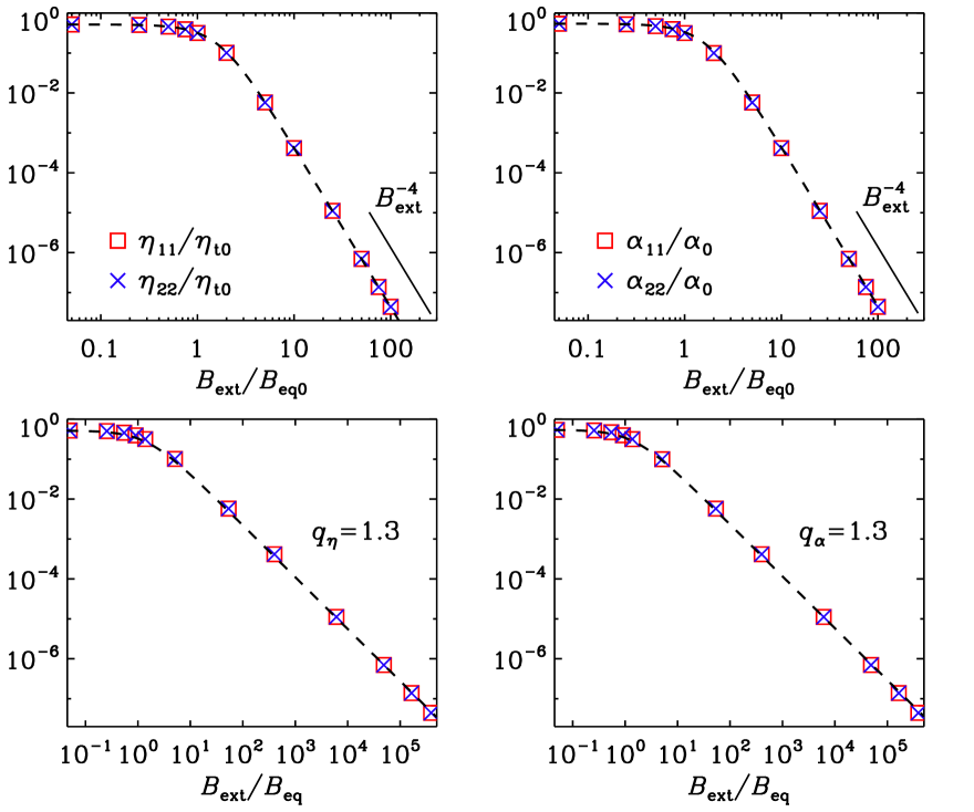
Figure 1.— Results of Set RF1, $R_{\mathrm{m0}}=0.88$: Variations of $\eta_{11}$, $\eta_{22}$ (left) and $\alpha_{11}$, $\alpha_{22}$ (right) with the external magnetic field in the $x$ direction. Top: dependences on $B_{\rm ext}/B_{\rm eq0}$ with fit (31). Bottom: dependences on $B_{\rm ext}/B_{\rm eq}$ with fit (32). Fits dashed.

The condition for Re can be relaxed when rewriting the advective terms in the second-order momentum equation in the form $\left(\mbox{\boldmath$\nabla$}{}\times\bm{{{u}}}^{(2)}\right)\times\bm{{{u}}}_{0}+(\mbox{\boldmath$\nabla$}{}\times\bm{{{u}}}_{0})\times\bm{{{u}}}^{(2)}+\mbox{\boldmath$\nabla$}{}\left(\bm{{{u}}}^{(2)}\cdot\bm{{{u}}}_{0}\right)$. A solution $\bm{{{u}}}^{(2)}\sim\bm{{{u}}}_{0}$ can already exist (approximately), if the sum of magnetic and dynamical pressure, $\bm{{{b}}}^{(1)}\cdot\bm{B}_{\rm ext}+\rho_{0}\bm{{{u}}}^{(2)}\cdot\bm{{{u}}}_{0}$, is negligible compared to $p_{0}=c_{\rm s}^{2}\rho_{0}$, more precisely and less restricting, if the non-constant part of this sum is negligible. At higher orders there is an increasing number of contributions to be taken into account.

Therefore, following the definition (24), we can define $\alpha\approx\alpha_{11}\approx\alpha_{22}$ and $\eta_{\rm t}\approx\eta_{11}\approx\eta_{22}$. The transport coefficients start to be quenched when $B_{\rm ext}$ exceeds $B_{\rm eq0}$ or $B_{\rm eq}$ and seem to follow a power law for strong fields. To compare with earlier works, it is useful to consider the dependences on $B_{\rm ext}/B_{\rm eq0}$. Calculating the quenched coefficients under SOCA by a power series expansion with respect to $B_{\rm ext}$, only the even powers occur. Accordingly, we find that our data fit remarkably well with

$$\sigma=\frac{\sigma_{0}}{1+p_{\sigma 1}(B_{\rm ext}/B_{\rm eq0})^{2}+p_{\sigma 2}(B_{\rm ext}/B_{\rm eq0})^{4}}\,,$$ (31)

where $\sigma$ stands for $\alpha$ or $\eta_{\rm t}$ and $p_{\sigma 1}=0.51$ and $p_{\sigma 2}=0.12$; see upper panels of Figure 1. Therefore our results are consistent with those of SBS07 and RB10 who found asymptotically the power $4$ for steady forcing.

Alternatively, we may consider the dependences on $B_{\rm ext}/B_{\rm eq}$ which are weaker, because the actual $B_{\rm eq}$ is itself quenched. We find as an adequate model

$$\sigma=\frac{\sigma_{0}}{1+p_{\sigma}(B_{\rm ext}/B_{\rm eq})^{q_{\sigma}}}\quad\mbox{(for $\sigma=\alpha$ or $\eta_{\rm t}$)}$$ (32)

with $q_{\alpha}\approx q_{\eta}\approx 1.3$ and $p_{\alpha}\approx p_{\eta}\approx 0.59$; see lower panels of Figure 1. From now onward we shall consider the dependences on $B_{\rm ext}/B_{\rm eq}$ and stick to the fitting formula (32). We have performed another set of simulations with different parameters (RF2 in Table 1) and also at different wavenumbers of the test-fields. In all the cases we get the same quenching behavior.

The obtained isotropy of the quenched coefficients seems to be in conflict with the results of RB10, who detected strong anisotropy in $\alpha_{ij}$ for Roberts I forcing. However, the analytic consideration above makes clear, that this was a consequence of their use of a simplified momentum equation missing the pressure term. Thus, the ingredient just necessary to allow the flow keeping its geometry while being influenced by the imposed field, was missing. One may speculate though, that for more compressive flows the anisotropy may become larger.

Table 1Summary of the runs.

Set	Description	${\hat{\bm{{B}}}}_{\rm ext}$	TFM	$R_{\mathrm{m0}}\;$	$R_{\mathrm{m}}^{\rm min}$		$\>P_{\mathrm{m}}$	$B_{\rm eq0}$		$p_{\alpha}$	$p_{\gamma}$	$p_{\eta}$	$p_{\delta}$	$q_{\alpha}$	$q_{\gamma}$	$q_{\eta}$	$q_{\delta}$
RF1	Forced Roberts flow	$\hat{\bm{x}}$	TFZ	0.88	0.0002		1.0	0.010		0.59	-	0.59	-	1.3	-	1.3	-
RF2	Forced Roberts flow	$\hat{\bm{x}}$	TFZ	0.707	0.10		1.0	1.000		0.3	-	0.4	-	1.3	-	1.3	-
TBx	Forced turbulence ($k_{\mathrm{f}}=5k_{1}$)	$\hat{\bm{x}}$	TFZ	0.87	0.71		1.0	0.045		-	-	0.38	-	-	-	1.1	-
TBz	Forced turbulence ($k_{\mathrm{f}}=5k_{1}$)	$\hat{\bm{z}}$	TFZ	0.87	0.71		1.0	0.045		-	-	0.21	-	-	-	1.1	-
AT1	Forced turbulence ($k_{\mathrm{f}}=27k_{1}$)	$\hat{\bm{z}}$	TFA	2.23	1.67		1.0	0.060		-	-	0.66	-	-	-	1.2	-
AT2	Forced turbulence ($k_{\mathrm{f}}=27k_{1}$)	$\hat{\bm{z}}$	TFA	18.2	15.8		1.0	0.100		-	-	2.50	-	-	-	1.0	-
AT3	Forced turbulence ($k_{\mathrm{f}}=27k_{1}$),	$\hat{\bm{z}}$	TFA		0.08		1.0	0.022		-	-	-	-	-	-	-	-
	Fo$B_{\rm ext}/B_{\rm eq}\approx 4.3$ fixed				– 537			– 0.116
CR0	Non-rotating convection	$\hat{\bm{z}}$	TFZ	3.91	0.5		0.8	0.087		-	0.34	0.34	-	-	1.2	1.2	-
CR1	Rotating convection	$\hat{\bm{x}}$	TFZ	3.85	0.7		0.8	0.087		0.11	0.12	0.20	0.02	1.8	1.4	1.3	2.0
CR2	Rotating convection	$\hat{\bm{x}}$	TFZ	11.7	0.2		5.0	0.054		0.14	0.11	0.10	0.06	1.8	1.3	1.3	1.8
CR3	Rotating convection	$\hat{\bm{x}}$	TFZ	20.2	6.0		3.0	0.090		0.25	0.24	0.65	0.06	2.0	1.3	1.3	2.0
CR4	Rotating convection	$\hat{\bm{x}}$	TFZ	29.1	3.3		5.0	0.065		0.17	0.15	0.16	0.07	2.0	1.3	1.3	1.8
CR5	Rotating convection	$\hat{\bm{x}}$	TFZ	89.5	19.2		5.0	0.082		0.24	0.23	0.37	0.12	1.8	1.24	1.26	1.7
CR1Bz	As CR1	$\hat{\bm{z}}$	TFZ	3.85	0.13		0.8	0.088		0.65	0.12	0.41	1.0	1.3	1.3	1.3	1.8
CR3Bz	As CR3	$\hat{\bm{z}}$	TFZ	28.6	0.08		5.0	0.065		0.59	0.21	0.41	0.25	1.3	1.4	1.3	2.0
CR6	As CR1, uniform test fields	$\hat{\bm{x}}$	TFZ	3.85	0.70		0.8	0.087		0.16	0.11	-	-	2.0	1.4	-	-
CR7	As CR2, uniform test fields	$\hat{\bm{x}}$	TFZ	29.1	3.2		5.0	0.065		0.16	0.16	-	-	2.0	1.3	-	-

Note. — Data given for the stationary (Sets RF1 and RF2) or statistically saturated state, respectively. $q_{\alpha}$, $q_{\gamma}$, $q_{\eta}$, and $q_{\delta}$ are the quenching exponents for $\alpha$, $\gamma$, $\eta_{\rm t}$, and $\delta$, respectively, according to Equation (32). For RF1: $u_{0}=0.01c_{\rm s},\eta=0.008c_{\rm s}/k_{1}$, RF2: $u_{0}=1.0c_{\rm s},\eta=c_{\rm s}/k_{1}$, CR0: $\mbox{\rm Ra},\Pr=3\times 10^{5},3.95$, CR1: $\mbox{\rm Ta},\mbox{\rm Ra},\Pr=5.6\times 10^{3},3\times 10^{5},3.95$, CR2: $\mbox{\rm Ta},\mbox{\rm Ra},\Pr=6.4\times 10^{5},3\times 10^{5},4.94$, CR3: $\mbox{\rm Ta},\mbox{\rm Ra},\Pr=1.0\times 10^{4},4\times 10^{5},2.93$, CR4: $\mbox{\rm Ta},\mbox{\rm Ra},\Pr=2.6\times 10^{6},5\times 10^{5},2.44$, CR5: $\mbox{\rm Ta},\mbox{\rm Ra},\Pr=1.6\times 10^{7},1\times 10^{6},0.97$. Resolutions used are RF1: $96^{3}$, RF2: $144^{3}$, TBx, TBz: $256^{3}$, AT1: $128^{3}$, AT2: $360^{3}$, AT3: $72^{3}$ to $672^{3}$ CR0-CR7: $128^{3}$. $R_{\mathrm{m}}^{\rm min}$ – minimal, i.e., maximally quenched $R_{\mathrm{m}}$ within a Set.