ALMA observations of a candidate molecular outflow in an obscured quasar

Abstract

We present Atacama Large Millimeter/Submillimeter Array (ALMA) CO (1-0) and CO (3-2) observations of SDSS J135646.10+102609.0, an obscured quasar and ultra-luminous infrared galaxy (ULIRG) with two merging nuclei and a known 20-kpc-scale ionized outflow. The total molecular gas mass is $M_{\rm{mol}}\approx 9^{+19}_{-6}\times 10^{8}$ $M_{\odot}$, mostly distributed in a compact rotating disk at the primary nucleus ($M_{\rm{mol}}\approx 3\times 10^{8}$ $M_{\odot}$) and an extended tidal arm ($M_{\rm{mol}}\approx 5\times 10^{8}$ $M_{\odot}$). The tidal arm is one of the most massive molecular tidal features known; we suggest that it is due to the lower chance of shock dissociation in this elliptical/disk galaxy merger. In the spatially resolved CO (3-2) data, we find a compact ($r\approx 0.3$ kpc) high velocity ($v\approx 500$ km s^-1) red-shifted feature in addition to the rotation at the N nucleus. We propose a molecular outflow as the most likely explanation for the high velocity gas. The outflowing mass of $M_{\rm{mol}}\approx 7\times 10^{7}$ $M_{\odot}$ and the short dynamical time of $t_{\rm{dyn}}\approx 0.6$ Myr yield a very high outflow rate of $\dot{M}_{\rm{mol}}\approx 350$ $M_{\odot}$ yr^-1 and can deplete the gas in a million years. We find a low star formation rate ($<16$ $M_{\odot}$ yr^-1 from the molecular content and $<21$ $M_{\odot}$ yr^-1 from the far-infrared spectral energy distribution decomposition) that is inadequate to supply the kinetic luminosity of the outflow ($\dot{E}\approx 3\times 10^{43}$ ergs s^-1). Therefore, the active galactic nucleus, with a bolometric luminosity of $10^{46}$ ergs s^-1, likely powers the outflow. The momentum boost rate of the outflow ($\dot{p}/(L_{\mathrm{bol}}/c)\approx$3) is lower than typical molecular outflows associated with AGN, which may be related to its compactness. The molecular and ionized outflows are likely two distinct bursts induced by episodic AGN activity that varies on a time scale of $10^{7}$ yr.

1. Introduction

In the past decade, supermassive black holes (BHs) have been found to be a common constituent of galaxy centers (e.g., Kormendy & Ho, 2013). At the same time, we have come to appreciate that supermassive BHs may play an active role in shaping galaxy evolution through feedback in the active galactic nucleus (AGN) phase (e.g., Fabian, 2012). The steep high-mass cut-off in the galaxy luminosity function (e.g., Bower et al., 2006) and the over-production of massive blue galaxies in cosmological simulations (e.g., Croton et al., 2006) requires a mechanism to quench star formation at the high-mass end. The enormous amount of energy released by black hole accretion provides a way to heat up or expel gas on galaxy-wide scales (e.g., Ciotti & Ostriker, 2001; Faucher-Giguère & Quataert, 2012). This kind of AGN feedback may regulate star formation (e.g., Page et al., 2012) and/or BH growth (e.g., Booth & Schaye, 2010) in a way that links the evolution of the BH and the galaxy and results in the local BH scaling relations (e.g., McConnell & Ma, 2013; Kormendy & Ho, 2013; Sun et al., 2013).

The actual mechanisms that link the AGN with galaxy-scale gas remain unknown. There have been many studies searching for outflows in different gas phases, including X-ray emitting hot gas (e.g., Wang et al., 2009, 2011; Greene et al., 2014), warm ionized (e.g., Stockton & MacKenty, 1987; Whittle, 1992; Nesvadba et al., 2006; Fu & Stockton, 2008; Greene et al., 2011; Villar-Martin et al., 2011; Rupke & Veilleux, 2013; Yuma et al., 2013; Liu et al., 2013a; Hainline et al., 2013; Villar-Martin et al., 2014; Zakamska & Greene, 2014), neutral (e.g., Rupke et al., 2005; Teng et al., 2013), and cold molecular gas (e.g., Walter et al., 2002; Feruglio et al., 2010; Alatalo et al., 2011; Sturm et al., 2011; Aalto et al., 2012; Flower & Pineau des Forets, 2013; Feruglio et al., 2012; Veilleux et al., 2013; Cicone et al., 2014). As has been shown by these studies, AGN-driven outflow is a complex phenomenon involving gas at a wide range of temperatures, densities, and distributions. Identifying the driving mechanism of the outflow, e.g. star formation or AGN, is challenging in many cases, in particular because of ambiguities between star formation and AGN activity indicators. Therefore, multi-wavelength observations are essential to put together a comprehensive picture of AGN feedback.

Only recently have we come to appreciate the ubiquity of molecular outflows. They are commonly seen in Herschel OH spectroscopy (e.g., Sturm et al., 2011; Veilleux et al., 2013). Also, exciting evidence from interferometric observations suggest that these molecular outflows are massive, with a high mass loss rate that can deplete the cold gas in the galaxy in $10^{6}-10^{8}$ yr (e.g., Feruglio et al., 2010; Alatalo et al., 2011; Cicone et al., 2014). As molecular gas is the fuel for star formation, monitoring the molecular content in the host galaxy is key to determining whether or not the AGN can quench star formation and shape galaxy evolution.

In this paper, we inspect the molecular properties of the obscured quasar
SDSS J135646.10+102609.0 (SDSS J1356+1026 hereafter) with the Atacama Large Millimeter/Submillimeter Array (ALMA), looking for traces of the impact of the AGN on the cold gas component in the galaxy. SDSS J1356+1026 is an example of feedback in action; an extended and energetic outflow is detected in ionized gas that is most likely AGN-driven (Greene et al., 2012). The spatially resolved ALMA CO (1-0) and CO (3-2) observations presented here allow us to constrain the morphology, kinematics, and mass of the molecular gas and to investigate the relation between the molecular gas and the ionized outflow.

Throughout, we assume $h=H_{0}/100$ km s^-1 Mpc^-1 = 0.7, $\Omega_{\rm{m}}=0.3$, and $\Omega_{\mathrm{\Lambda}}=0.7$. At the redshift of the object (z=0.1231), 1″  corresponds to 2.2 kpc, and the luminosity distance is 580 Mpc. All velocities used in this paper are in the heliocentric frame using the optical velocity convention. Wavelengths are expressed in vacuum.

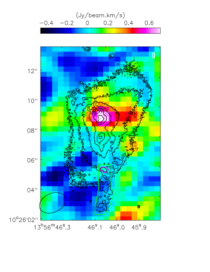
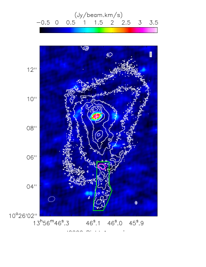
Figure 1.— Integrated line intensity (moment-0) maps for SDSS J1356+1026 in CO (1-0) (left) and CO (3-2) (right) are shown in color. These moment-0 maps are integrated over a velocity range of $-300$ to $+300$ km s^-1. $1~{}\sigma$ noise level is $0.15$ Jy beam^-1 km s^-1 and 0.16 Jy beam^-1 km s^-1 for CO (1-0) and CO (3-2) respectively. The beam ellipse is shown in the lower left corner. Contours show intensity of optical emission as seen in the HST/WFC3 F814W $I-$band images and are spaced by a factor of two in intensity. The bold letters in the left panel indicate the three major components, the N/S nucleus and the W arm. The CO emission is most prominent at the N nucleus and the W arm $2\arcsec$ to the west of the N nucleus. Emission at the S nucleus is also detected in CO (1-0) in certain channels, see Fig. 3. The red clump at the bottom of the CO (1-0) map is noise at 3 $\sigma$ level. The green region marks the the ionized outflow, and the magenta region is its base. There is no detection of a CO counterpart to the extended (10 kpc) ionized [O III] outflow. The red line across the N nucleus on the right panel indicates the $pv$-diagram cut (Fig. 7).

1.1. SDSS J1356+1026

SDSS J1356+1026 is a merging system at z=0.123 classified as a luminous obscured (Type 2) quasar with a bolometric luminosity $L_{\mathrm{bol}}$$\approx 10^{46}$ ergs s^-1 inferred from the [O III]  luminosity, $L_{\mathrm{[O{\tiny III}]}}$= $10^{42.77}$ ergs s^-1 (Greene et al., 2009; Liu et al., 2009). It is also an ultra-luminous infrared galaxy (ULIRG; $L_{\rm{FIR}}=2.68\pm 0.53\times 10^{45}$ ergs s^-1). The radio continuum is unresolved with a luminosity density of $\nu L_{\nu}=3.4\times 10^{40}$ ergs s^-1 from the VLA FIRST survey at 1.4 GHz (1.6 GHz rest frame), indicating that it is a radio-quiet quasar (Greene et al., 2012). The coordinate of SDSS J1356+1026 is (13:56:46.10, +10:26:09.09).

The two merging galaxies, which we refer to as the northern (N) and southern (S) nuclei, are separated by 2.5 kpc ($1\farcs 1$). The N nucleus is detected at 2-10 keV and is the primary AGN host in the system (Greene et al. 2014). Both the total molecular mass (Section 3.3) and the r-band light (Greene et al., 2009) are dominated by the northern nucleus, with a ratio of $\sim 4:1$ (N:S). The progenitor of the northern galaxy is likely a moderately massive early-type galaxy, with a stellar spectrum that is dominated by an old stellar population and a stellar velocity dispersion $\sigma_{*}=206\pm 36$ km s^-1 (Greene et al., 2009), corresponding to a stellar mass $M_{*}\approx 10^{11}$ $M_{\odot}$  (Hyde & Bernardi, 2009), and the black hole mass is estimated to be $M_{\rm BH}\approx 3\times 10^{8}$ $M_{\odot}$  ($\pm 0.38$ dex, McConnell & Ma, 2013). The corresponding Eddington luminosity is $L\mathrm{{}_{Edd}}$$=3.1\times 10^{46}$ ergs s^-1 ($\pm 0.38$ dex), which yields an Eddington ratio range of 0.1-1, energetic enough to drive a hot wind (e.g., Veilleux et al., 2005).

The most spectacular feature of this system is an [O III]-emitting bubble extending $\sim 10$ kpc to the south of the nuclei (green region in Fig. 1), with a weaker symmetric counterpart to the north. Long-slit spectroscopy along the ouflow reveals the distinctive double-peaked spectrum of an expanding shell. A simple geometric model yields a deprojected velocity $v\approx 1000$ km s^-1, a dynamical time $t_{\rm{dyn}}\approx 10^{7}$ yr, and a kinetic luminosity $\dot{E}\approx 10^{44-45}$ ergs s^-1 (Greene et al., 2012). As the radio emission is compact and faint (Sec. 3.1, 5.2.2), and the star formation rate is low (Sec. 3.3, 3.4), this ionized outflow provides a strong case for a quasar-driven wind (Greene et al., 2014).

2. Observations

2.1. ALMA CO (1-0) and CO (3-2) Observations

The ALMA CO (1-0) and CO (3-2) observations were conducted during Cycle 0 and Cycle 1 under project codes 2011.0.00652.S and 2012.1.00797.S respectively. The CO (1-0), at sky frequency 102.6 GHz, was observed in band 3 in two blocks on May 9 and July 30, 2012, using 16 and 23 12-m antennae for 68 and 63 minutes respectively (27 and 24 minutes on-source). The CO (3-2) at 307.9 GHz was observed in band 7 on July 6, 2013 with twenty-seven 12-m antennae in 24 minutes (19 minutes on-source). In the following, CO (1-0) properties are followed by CO (3-2) in parenthesis. Both lines use a single pointing covering the whole system with a field of view of 62″  (21″), and dual polarizations. They use the same spectral set-up with a total bandwidth of 2 GHz divided into 128 channels, each 15.625 MHz wide, corresponding to a channel width of 46 km s^-1  (15 km s^-1). The CO (1-0) data has an additional spectral window at 93 GHz. The channels are Hanning-smoothed within the correlator. QSO 3C279 (J1516+0015), Mars (Titan), and J1415+133 (J1347+1217) were used for the bandpass, flux, and phase calibrators respectively. The phase calibrator is observed for 30 (90) seconds every 11 (9) minutes. The absolute flux calibration accuracy is 5% for CO (1-0) (Band 3) and 10% for CO (3-2) (Band 7).

The data calibration was carried out by the ALMA team using CASA version 3.3.0 for CO (1-0) and 4.1.0 for CO (3-2). We further used CASA version 4.1.0 to apply continuum subtraction [CO (1-0) only], heliocentric correction, imaging, and cleaning. For CO (1-0), the continuum level was estimated from line free channels (36/43 channels on the blue/red side) and subtracted in the uv-plane. Continuum subtraction was not applied to the CO (3-2) data cube as there are not enough line-free channels to determine the continuum level. However, we extrapolate from the 100 GHz and 1.4 GHz continuum flux densities (spectral index $\alpha=-0.86$, Sec. 3.4) to estimate a 300 GHz flux density of 0.58 mJy. This extrapolated continuum level is lower than the noise level in each CO (3-2) channel and is less than 10% of the emission line flux density at the N nucleus. The CO (3-2) channel is further binned by two to increase the SNR in each channel, giving a final channel width of 30 km s^-1, while the CO (1-0) channel width is unchanged (46 km s^-1).

The imaging processing was carried out with the CASA task clean. We used the Briggs visibility weighting with a robustness parameter of 0.5 (Briggs, 1995), which is a compromise between maximum resolution and maximum sensitivity. The beam size is $\theta_{\rm{beam}}=1\farcs 9\times 1\farcs 3~{}(0\farcs 35\times 0\farcs 29)$ with a PA=$-62^{\circ}~{}(-60^{\circ})$, and the maximum resolvable scale is $\theta_{\rm{MRS}}=29\arcsec~{}(10\arcsec)$. All images are cleaned to the 3 $\sigma$ level in each channel. The resulting RMS noise level in each channel is 0.37 mJy beam^-1 (0.77 mJy beam ^-1).

Table 1 Flux Measurements

		CO (1-0)			CO (3-2)
Name	$\Delta v$	$S_{\nu}\Delta v$	$L$	$L^{\prime}$	$S_{\nu}\Delta v$	$L$	$L^{\prime}$
	(km s-1)	(Jy km s-1)	($10^{3}L_{\odot}$)	($10^{9}$ K km s-1pc2)	(Jy km s-1)	($10^{3}L_{\odot}$)	($10^{9}$ K km s-1pc2)
(1)	(2)	(3)	(4)	(5)	(6)	(7)	(8)
N Nucleus	$-300$ : 500	$0.46\pm 0.27$	$16.6\pm 9.6$	$0.34\pm 0.19$	$4.90\pm 0.22$	$528\pm 24$	$0.40\pm 0.02$
N Outflow	300 : 500	$0.06\pm 0.08$	$2.2\pm 2.7$	$0.04\pm 0.06$	$0.99\pm 0.10$	$107\pm 11$	$0.08\pm 0.01$
S Nucleus	$-80$ : 50	$0.13\pm 0.06$	$4.5\pm 2.2$	$0.09\pm 0.04$	$0.11\pm 0.07$	$12\pm 7$	$0.01\pm 0.01$
W Arm	$-300$ : 500	$0.82\pm 0.34$	$29.3\pm 12.2$	$0.60\pm 0.25$	$2.55\pm 0.40$	$275\pm 44$	$0.21\pm 0.03$
Sum		$1.40\pm 0.44$	$50.4\pm 15.7$	$1.03\pm 0.32$	$7.57\pm 0.46$	$815\pm 50$	$0.62\pm 0.04$

Note. — The CO (1-0) and CO (3-2) fluxes and derived properties of the main components (Sec. 3.2). Columns 3 to 5 pertain to CO (1-0) and columns 6 to 8 pertain to CO (3-2). The last row is a sum of the three components: the N/S nuclei and the W arm. The listed errors correspond to the RMS noise in the data. In addition, there is a 5% and 10% flux calibration error for CO (1-0) and CO (3-2) respectively. The CO (1-0) flux errors of the N nucleus and W arm also include errors due to source decomposition. Column 1: component. Column 2: the velocity range over which the flux is integrated. Column 3: integrated CO (1-0) flux. Column 4: the CO (1-0) line luminosity, adopting a luminosity distance of 580 Mpc. Column 5: the emitting area and velocity integrated CO (1-0) source brightness temperature. Column 6: integrated CO (3-2) flux. Column 7: the CO (3-2) line luminosity, adopting a luminosity distance of 580 Mpc. Column 8: the emitting area and velocity integrated CO (3-2) source brightness temperature.

2.2. Matching ALMA with Optical Data

In order to compare the molecular and stellar components of the galaxies, we match the ALMA data cube to the SDSS spectrum in velocity and the Hubble Space Telescope HST/WFC3 F814W ($I-$band) image in position (Comerford et al. in prep.). We use the SDSS DR7 spectrum (Abazajian et al., 2009), which was taken in a 3$\arcsec$ aperture with a spectral resolution of FWHM $\approx$ 150 km s^-1 centered on the N nucleus. The HST/WFC3 F814W image was observed on May 19 2012 with an integration time of 900 seconds and resolution of $0\farcs 07$.

To perform positional alignment, we identify another galaxy SDSS J135646.50+102553.6 that appears in the ALMA, SDSS, and HST images, and two other fainter galaxies in both SDSS and HST. We found that while the ALMA and SDSS positions are well-matched, there is a $0\farcs 6$ offset from the HST position. After applying this offset to the HST image, the ALMA (continuum) and HST coordinates of the northern nucleus are aligned well within $0\farcs 04$, much smaller than the ALMA CO (3-2) beam size ($0\farcs 35\times 0\farcs 29$). Rotation and stretching of the HST image with respect to the SDSS coordinates are also constrained to be within $0.4^{\circ}$ rotation and $0.5\%$ stretching.

The velocities in this paper are with respect to the rest frame of the stellar absorption features of N galaxy. We define the systemic velocity to be the best-fit redshift (z = 0.1231) from the SDSS spectrum, which is dominated by the light of the N nucleus, as the N nucleus is brighter and the fiber is centered on it. Both the stellar absorption and AGN emission lines are fitted by the SDSS template. A redshift warning flag ”many outliers” is raised, indicating that the template cannot capture the multi-component emission lines, but this is not a major concern for redshift accuracy. As a sanity check, we refit the stellar continuum using Bruzual & Charlot (2003) stellar population synthesis templates and the best-fit redshift differs from that of the SDSS by $-30$ km s^-1. We therefore adopt a redshift error of $\delta z=\pm 0.0001$ ($\pm$ 30 km s^-1). This stellar continuum fitting also reveals that the light in the N nucleus is dominated by old stellar populations, as discussed in Greene et al. (2009).

Figure 2.— SDSS J1356+1026 CO (1-0) (left) and CO (3-2) (right) channel maps in color. Each of the channel maps is 100 km s^-1 wide in velocity. The 1-$\sigma$ noise level of the image is 0.31 mJy beam^-1 km s^-1 and 0.32 mJy beam^-1 km s^-1 for CO (1-0) and CO (3-2) respectively. The beam ellipse is shown in the lower left corner. Contours show intensity of optical emission as seen in the HST/WFC3 F814W $I-$band images and are spaced by a factor of two in intensity. The N nucleus is prominent with a wide velocity range between $-300$ to 500 km s^-1 especially in the CO (3-2) maps. The W arm is strong in two channels $-200$ and $-100$ km s^-1, and the S nucleus can be seen at 0 km s^-1 in the CO (1-0) maps.

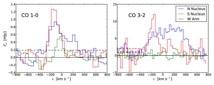
Figure 3.— CO (1-0) (left) and CO (3-2) (right) spectra of the N/S nucleus and the W arm. The N nucleus has wide line width in both CO (1-0) and CO (3-2), and the peak at $-100$ km s^-1 in the CO (1-0) spectrum is contamination from the W arm. The W arm has relatively narrow line width, reflecting its coherent kinematics structure across the arm. The S nucleus is fainter and is detected only in CO (1-0). The dashed horizontal lines indicate the 1 $\sigma$ noise level. To avoid contamination between sources, the CO (1-0) spectra are integrated only over one beam size, and therefore do not include all the flux in the sources. The CO (3-2) spectra are integrated over regions at least twice as large as the beam, and therefore contains $\sim 95\%$ of the flux in the N nucleus.

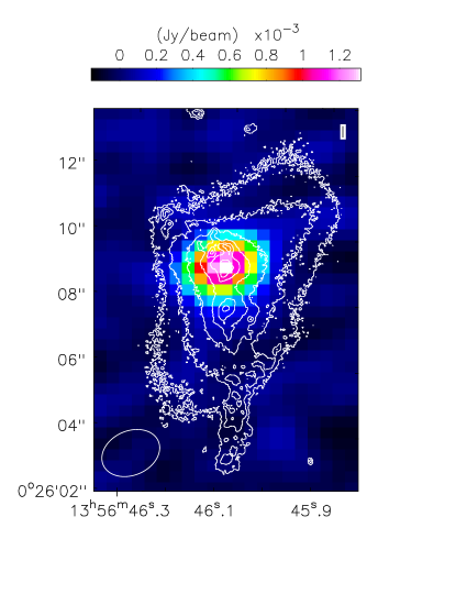
Figure 4.— 100 GHz radio continuum image (color) overlaid with the HST/F814W image (contour). The contours of the HST image are in log scale; each contour differs by a factor of 2. The radio image is made from line-free channels at the two spectral windows of 93/103 GHz (rest-frame 104/115 GHz), each 2 GHz wide. There is one unresolved radio continuum source associated with the N nucleus, likely from the AGN (see Fig. 5).

3. Analysis

In this section, we describe our procedures to estimate the 100 GHz continuum flux density, CO (1-0) and CO (3-2) line fluxes, molecular gas masses, the star formation rate, and the AGN bolometric luminosity. The measurements are summarized in Tables 1 and 2, and will be discussed in Section 4.

We first introduce the three major components in the CO data: the N nucleus, the S nucleus, and the Western arm (W). All three are spatially coincident with optical features. The N nucleus has strong emission from both CO (1-0) and CO (3-2), as seen in the integrated line intensity maps (moment-0, Fig. 1) and the channel maps (Fig. 2) with a very broad spectrum (Fig. 3). The S nucleus is not detected in CO (3-2), but is seen in CO (1-0) (Fig. 3). To the west of the N nucleus is another strong blue-shifted and extended emission feature in both transitions, which we call the W arm. This feature overlaps with an extended stellar plume in the HST images, and has blue-shifted but narrow CO lines. Other than these three main components, no prominent CO emission is detected. There is no large-scale molecular gas associated with the [O III] outflow discovered by Greene et al. (2012), but there is a low significance (3 $\sigma$) double-peaked CO (3-2) emission component at the base of the [O III] expanding bubble (Sec. 4.4).

3.1. 100 GHz Continuum

The radio 100 GHz continuum is measured from the line-free channels in two spectral windows at 93/103 GHz (rest-frame 104/115 GHz) in the CO (1-0) data. The moment-0 map (Fig. 4) shows an unresolved point source with a beam size of $1\farcs 9\times 1\farcs 3$ ($4.2\times 2.9$ kpc) at the N nucleus with a flux density of $1.51\pm 0.07\pm 0.07$ mJy. The first error is from the RMS noise, and the second is the 5% calibration error. The spectral energy distribution of SDSS J1356+1026 including this 100 GHz flux density is discussed in Section 3.4.

3.2. CO Flux Measurements

We extract the CO(1-0)/(3-2) spectra (flux densities $F_{\mathrm{\nu}}$, Fig. 3), and fluxes ($F=F_{\mathrm{\nu}}\Delta v$, Table 1) for the three components (the N/S nuclei and the W arm) from the cleaned data. In addition to the RMS noise errors presented in Fig. 3 and Table 1, there is a 5 % and 10 % flux calibration error for the CO (1-0) and CO (3-2) data respectively. We start with the CO (3-2) data as it has higher resolution to spatially separate the components. We use simple aperture photometry with apertures at least twice as large as the beam in order to enclose $\mathrel{\hbox{\hbox to0.0pt{\hbox{\lower 4.0pt\hbox{$\sim$}}\hss}\hbox{\raise 2.0pt\hbox{$>$}}}}95\%$ of the flux. As the N and W apertures are adjacent to each other, we expect flux contamination between these two components at a level of 10% or less for CO (3-2). The S aperture is well-separated from the other two sources and does not overlap with side-lobes of the N nucleus.

Assuming Gaussian noise correlated on the scale of the beam, we estimate the errors in the spectra $F_{\nu}$ based on the image noise level rms($I_{\nu}$), taken from large emission-free regions, the beam $\mathrm{B}(\boldsymbol{r})$, a 2D Gaussian with peak value 1, and the aperture $T(\boldsymbol{r}$) = 1 inside the aperture and zero everywhere else, adopting the following equation:

$$\mathrm{rms}(F_{\nu})=\mathrm{rms}(I_{\nu})\sqrt{\int\int\mathrm{B}(\boldsymbol{r}_{2}-\boldsymbol{r}_{1})T(\boldsymbol{r}_{1})T(\boldsymbol{r}_{2}){\rm d}^{2}\boldsymbol{r}_{1}{\rm d}^{2}\boldsymbol{r}_{2}}.$$ (1)

To obtain the fluxes $F$, we integrate the spectra $F_{\nu}$ over a velocity range of $-300$ km s^-1$<v<$ 500 km s^-1 for the N nucleus and W arm, which is chosen as the velocity width where the CO (3-2) flux density is detected with greater than 2 $\sigma$ significance from the N nucleus. A velocity range of 300 km s^-1$<v<$ 500 km s^-1 is used for the high velocity component of the N nucleus. For the S nucleus, although there is no CO (3-2) detection, we use the velocity range $-80<v<50$ which covers the $>1~{}\sigma$ CO (1-0) emission. While estimating the errors in the fluxes, we take into account the correlation between adjacent channels, which has a Pearson correlation coefficient of $r=0.375$, due to Hanning smoothing during the observation and 2:1 binning in the image processing.

Estimating the CO (1-0) fluxes is more complicated, as the sources, especially the N nucleus and the W arm, are spatially blended. The CO (1-0) spectrum of the N nucleus clearly shows the narrow peak of the W arm at $-100$ km s^-1  (Fig. 3). However, we can still extract the uncontaminated N nucleus fluxes making use of their distinct spectral shape. We first estimate the N nucleus flux in the $100$ to $500$ km s^-1 channels that are free from W arm emission by fitting a model of the beam to the stacked moment-0 map of these channels. This point-source assumption should be valid as the CO (1-0) beam is much larger than the CO (3-2) N nucleus size. We then recover the total N nucleus CO (1-0) flux in the entire velocity range ($-300$ to $500$ km s^-1) assuming that the CO (1-0) spectrum has a similar spectral shape to the CO (3-2) spectrum.

The W arm CO (1-0) flux is then estimated as the difference between the total flux including both sources and the decomposed N nucleus flux. The CO (1-0) flux in the high velocity component of the N nucleus is estimated by the same point source fitting procedure over the velocity range of 300 to 500 km s^-1, as is the S nucleus over a velocity range of $-80$ to $50$ km s^-1, where the emission is seen. Correlations between adjacent channels are determined from emission-free regions and are taken into account for the flux error estimation. Using the estimated fluxes of the components in both lines, we express the line ratio as $L^{\prime}_{\mathrm{CO(3-2)}}/L^{\prime}_{\mathrm{CO(1-0)}}$ in Table 2, where $L^{\prime}$ is in units of K km s^-1 pc², proportional to the brightness temperature.

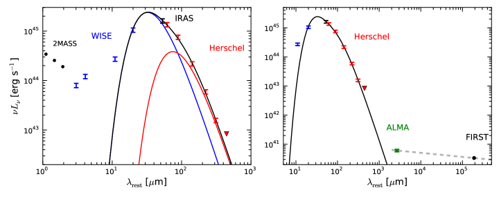
Figure 5.— Rest-frame spectral energy distribution of SDSS J1356+1026 (Sec. 3.4, Table 3). The black points are taken from the SED summarized by Greene et al. (2012). In addition, we include the WISE (blue), Herschel (red), and ALMA 100 GHz (green, Sec. 3.1) photometry. The solid black line shows the best-fit two-temperature modified black-body model fitted to the 22 µm WISE, 60 µm IRAS, and 70-350 µm Herschel data. The warm component (blue solid line) has a best-fit temperature of 81 K, while the temperature of the cold component (red solid line) is fixed at 35 K. The grey dashed line on the right panel links the ALMA 100 GHz and FIRST 1.4 GHz (from Greene et al., 2012) points with a spectral index of $\alpha=-0.86$ ($F_{\nu}\propto\nu^{\alpha}$).

Table 2Molecular Gas Properties

Name	$M_{\mathrm{mol}}$	$L^{\prime}_{\mathrm{CO(3-2)}}/L^{\prime}_{\mathrm{CO(1-0)}}$
	($M_{\odot}$)
(1)	(2)	(3)
N Nucleus	$3^{+6}_{-2}\times 10^{8}$	$1.18\pm 0.73$
N Outflow	$7^{+15}_{-5}\times 10^{7}$${}^{~{}a}$	$>0.45^{~{}b}$
S Nucleus	$<3.8\times 10^{8~{}c}$	$0.10\pm 0.11$
W Arm	$5^{+11}_{-3}\times 10^{8}$	$0.35\pm 0.20$
Sum	$9^{+19}_{-6}\times 10^{8}$	$0.60\pm 0.22$

Note. — The molecular gas properties. Column 1: component. Column 2: the molecular gas mass (Sec. 3.3). The errors are dominated by the 0.5 dex error in the X_CO factor. Column 3: the CO (3-2) to CO (1-0) ratio (Sec. 3.2), where $L^{\prime}$ is in unit of K km s^-1 pc². The errors are inferred from the RMS noise.

^a The molecular outflow mass is estimated from the CO (3-2) flux assuming $L^{\prime}_{\mathrm{CO(3-2)}}/L^{\prime}_{\mathrm{CO(1-0)}}=1$.

^b $3~{}\sigma$ lower-limit.

^c This is a conservative upper-limit inferred from the CO (1-0) 3 $\sigma$ detection limit and the X_CO uncertainty is taken into account.

3.3. Molecular Gas Mass and Star Formation Rate

From the measured CO (1-0) luminosity we can estimate the molecular gas mass (e.g., Bolatto et al., 2013). The masses are listed in Table 2. The CO-to-H₂ conversion factor X_CO  is defined as

$$X_{\mathrm{CO}}=N_{\mathrm{mol}}/W(\mathrm{CO(1-0)}),$$ (2)

where $N_{\mathrm{mol}}$ is the molecular column density in units of cm^-2, and $W(\mathrm{CO(1-0)}$) is the CO (1-0) brightness in units of K $\mathrm{km~{}s^{-1}}$. Although X_CO is roughly constant in normal Galactic molecular clouds (Solomon et al., 1987), it is found to be lower in ULIRG/starburst galaxies by a factor of 2-5 with large scatter (Downes & Solomon, 1998). Likely because the molecular clouds blend together due to tidal forces in the dense environment of the ULIRG nucleus, the CO emission emerges from a diffuse volume-filling medium rather than discrete self-gravitating molecular clouds.

SDSS J1356+1026 is identified as a ULIRG and has disturbed gas dynamics, so we adopt an X_CO value for ULIRGs X_CO= $0.4\times 10^{20}$ cm^-2 (K km s^-1)^-1 with an error of 0.5 dex (Downes & Solomon, 1998; Bolatto et al., 2013). This corresponds to $\alpha_{\rm{CO}}$= 0.86 $M_{\odot}$ (K kms pc²)^-1, matching the value used in other ULIRG/AGN CO studies (e.g., Cicone et al., 2014). This factor of three uncertainty in the X_CO factor dominates the errors in the mass estimates. We find a total molecular mass of $9^{+19}_{-6}\times 10^{8}~{}M_{\odot}$. Half of the molecular mass is in the extended W arm ($5^{+11}_{-3}\times 10^{8}~{}M_{\odot}$), while the N nucleus shares a third ($3^{+6}_{-2}\times 10^{8}~{}M_{\odot}$). As CO (1-0) is only marginally detected at the S nucleus, a conservative mass limit of $<3.8\times 10^{8}M_{\odot}$ is estimated from the 3 $\sigma$ detection limit and the uncertainty in X_CO.

Since molecular gas is the fuel for star formation, we can estimate the star formation that can be supported by the molecular content in SDSS J1356+1026. Using the Schmidt-Kennicutt law (Kennicutt, 1998), we find the star formation rate at the N nucleus to be SFR=1.2 $M_{\odot}$ yr^-1 ($\pm$ 0.5 dex) assuming that all of the molecular gas at the N nucleus is distributed in a disk with a radius of 300 pc, half of the beam deconvolved source FWHM in CO (3-2). As the morphology of the molecular gas in the W arm and the S nucleus are uncertain, their SFR is poorly constrained. A conservatively high estimate of the entire system can be calculated by putting all the molecular gas, including that in the diffuse W arm, in a disk with a radius of 300 pc, which gives 5 $M_{\odot}$ yr^-1. Taking the factor of three X_CO uncertainty into account, an absolute upper-limit is placed at 16 $M_{\odot}$ yr^-1. However, the star formation rate inferred from the CO luminosity is indirect. Whether the assumed X_CO factor and/or the Schmidt-Kennicutt law apply in this environment is uncertain. In the following section, we constrain the star formation rate directly from the infrared spectral energy distribution (SED) decomposition.

3.4. SED, Star Formation Rate and AGN Bolometric Luminosity

We use the infrared spectral energy distribution (SED) decomposition to constrain the star formation rate (Fig. 5, Table 3). It is usually thought that the dust close to the AGN is heated to much higher temperature than the diffuse dust heated by starlight. The difference in the dust temperatures is at the core of the SED-fitting method to distinguish between AGN-dominated and star formation-dominated sources. Greene et al. (2012) compiled a UV to radio spectral energy distribution (SED) of SDSS J1356+1026 making use of the 2MASS (Skrutskie et al., 2006), IRAS (Neugebauer et al., 1984), FIRST (Becker et al., 1995), and NVSS (Condon et al., 1998) data. We further include data from the Wide-field Infrared Survey Explorer WISE (Wright et al., 2010) and the Herschel Space Observatory (Pilbratt et al., 2010) PACS (Poglitsch et al., 2010) and SPIRE (Griffin et al., 2010) data from Petric et al. in prep., which extends to 500 µm to cover the Rayleigh-Jeans tail of the dust emission.

Following the decomposition procedures of Kirkpatrick et al. (2012) we fit a two-temperature modified blackbody to the seven-point SED. This SED of 22 µm WISE, 60 µm IRAS, and 70-350 µm Herschel is sensitive to the temperature of the dust emission. There are three free parameters in the model: the temperature $T_{\rm{warm}}$ and luminosity $L_{\rm{warm}}$ of the warm component and the luminosity of the cold component $L_{\rm{cold}}$. The temperature of the cold dust is fixed at $T_{\rm{cold}}=35$ K, as found in a wide range of systems by Kirkpatrick et al. (2012). Even if we fit the temperature of the cold component we recover $T_{\rm{cold}}=35$ K. The emissivity of the dust is assumed to be a power-law function of frequency with index $\beta=1.5$. All photometry errors are assumed to be 10%, which is representative of the systematic errors. The best-fit model (black line, Fig. 5) matches the data well with a reduced $\chi^{2}$ of 1. The best-fit temperature of the warm component is high $T_{\rm{warm}}=81$ K, and the luminosity is $L_{\rm{warm}}=2.6\times 10^{45}$ ergs s^-1, much higher than that of the cold component $L_{\rm{cold}}=4.3\times 10^{44}$ ergs s^-1.

The luminosity-weighted temperature $T_{\rm{eff}}=75$ K is higher than that seen in Kirkpatrick et al. (2012) even in those of their objects that have an AGN dominated SED ($T_{\rm{eff}}=65$ K). Therefore, as the warm component is consistent with being AGN-heated, the AGN is the major heating source for the bulk of the dust-emission. However, star-formation cannot be ruled out as the heating source for the 35 K cold component. We therefore use the luminosity of this 35 K component as an upper limit on the luminosity of dust emission associated with star formation, and use calibrations from Bell (2003) to calculate an upper limit on the star formation rate of 21 $M_{\odot}$ yr^-1. If the SFR were much higher, at the same $T_{\rm{cold}}$, the dust emission would exceed the measured 250 µm to 350 µm flux. This SFR upper-limit is insensitive to the temperature and luminosity of the warm component because the 250 µm and 350 µm  luminosities are dominated by the cold component. Harrison et al. (2014) estimated a higher star formation rate of $63^{+7}_{-17}$ $M_{\odot}$ yr^-1, inconsistent with our limit. This high SFR is inferred from the WISE and IRAS data alone covering 4.6 µm to 100 µm. In this case, the Herschel photometry at 250 µm and 350 µm are critical for the SED decomposition and SFR estimation.

We plot our measured 100 GHz flux (Sec. 3.1) in the SED (right panel of Fig. 5). The flux at 100 GHz is much higher than the extrapolated Rayleigh-Jeans tail of the dust emission, and thus must have a different origin. We find a spectral slope of $\alpha=-0.86$ ($F_{\rm{\nu}}\propto\nu^{\alpha}$) between the 100 GHz and the 1.4 GHz fluxes, similar to the typical spectral indices $\alpha\approx-0.7$ seen from synchrotron emission for radio-loud AGN (Zakamska et al., 2004).

Mid-infrared (5-25 µm) luminosity has also been used as a bolometric indicator for the AGN. We use the WISE photometry to infer $L_{\mathrm{bol}}$ following similar procedures as Liu et al. (2013b). As pointed out by Liu et al. (2013b), type 2 quasars have significantly redder mid-infrared colors than type 1 unobscured quasars, possibly due to dust reddening. This red color is also seen in SDSS J1356+1026. Therefore, to avoid attenuation from the dust, we choose the reddest WISE band at 22 µm  (19.5 µm  rest-frame) to apply the bolometric correction of $L_{\mathrm{bol}}=\nu L_{\nu}\times(11\pm 5)$ from Richards et al. (2006), which gives $L_{\mathrm{bol}}\approx 1.1\pm 0.5\times 10^{46}$ ergs s^-1. However, this $L_{\mathrm{bol}}$ might still be underestimated due to the strong extinction. We further use the 30 µm luminosity density extrapolated from the 3.4, 4.6, 12, and 22 µm data assuming a power-law spectral shape to set a conservative upper-limit of $L_{\mathrm{bol}}<2.3\times 10^{46}$ ergs s^-1 with a bolometric correction factor of 13 (Liu et al., 2013b). The $L_{\mathrm{bol}}$ estimate from the mid-infrared data is similar to that inferred from the [O III] luminosity, $L_{\mathrm{bol}}$$\approx 10^{46}$ ergs s^-1(Greene et al., 2012), using a $L_{\mathrm{bol}}$-$L_{\mathrm{[O{\tiny III}]}}$ relation (Liu et al., 2009) calibrated with type 1 AGN.

Table 3Spectral Energy Distribution

Band	$\lambda_{\rm{rest}}$	$\nu_{\rm{rest}}$	$\nu L_{\nu}$
	(µm)	(Hz)	($10^{44}$ ergs s-1)
(1)	(2)	(3)	(4)
WISE W1 3.4 µm	3.0	$9.9\times 10^{13}$	0.80
WISE W2 4.6 µm	4.1	$7.3\times 10^{13}$	1.21
WISE W3 12 µm	11	$2.8\times 10^{13}$	2.72
WISE W4 22 µma	20	$1.5\times 10^{13}$	10.5
IRAS 60 µma	53	$5.6\times 10^{12}$	16.1
Herschel PACS 70 µma	62	$4.8\times 10^{12}$	13.5
Herschel PACS 100 µma	89	$3.4\times 10^{12}$	7.50
Herschel PACS 160 µma	142	$2.1\times 10^{12}$	2.18
Herschel SPIRE 250 µma	223	$1.3\times 10^{12}$	0.59
Herschel SPIRE 350 µma	312	$9.6\times 10^{11}$	0.16
Herschel SPIRE 500 µm	445	$6.7\times 10^{11}$	$<$0.08
ALMA 100 GHz	$2.67\times 10^{3}$	$1.1\times 10^{11}$	$6.10\times 10^{-4}$

Note. — The rest-frame mid-to-far infrared spectral energy distribution of SDSS J1356 +1026 (Sec. 3.4, Fig. 5). Column 1: the telescope and band. Column 2: the rest frame wavelength. Column 3: the rest frame frequency. Column 4: the frequency times the luminosity density in the rest frame. The errors in the infrared data (WISE, IRAS, and Herschel) are assumed to be 10%.

^a The seven data points from the WISE 22µm to Herschel SPIRE 350 µm are used for the FIR SED decomposition fitting.

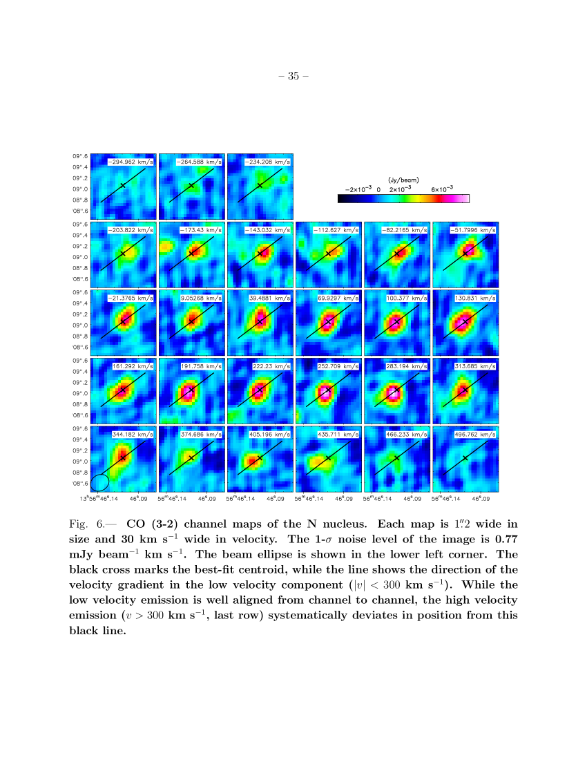
Figure 6.— CO (3-2) channel maps of the N nucleus. Each map is $1\farcs 2$ wide in size and 30 km s^-1 wide in velocity. The 1-$\sigma$ noise level of the image is 0.77 mJy beam^-1 km s^-1. The beam ellipse is shown in the lower left corner. The black cross marks the best-fit centroid, while the line shows the direction of the velocity gradient in the low velocity component ($|v|<300$ km s^-1). While the low velocity emission is well aligned from channel to channel, the high velocity emission ($v>300$ km s^-1, last row) systematically deviates in position from this black line.

4. Results

4.1. The N nucleus

There is strong CO (1-0) and CO (3-2) emission at the N nucleus with a wide velocity distribution from $-$300 km s^-1 to 500 km s^-1 (Fig. 3). From the CO (1-0) flux, the molecular gas mass is estimated to be $3^{+6}_{-2}\times 10^{8}$ $M_{\odot}$, which can fuel star formation at an approximate rate of $\sim$ 1 $M_{\odot}$ yr^-1, if the molecular gas is in a disk of radius 300 pc. The N nucleus has a CO line ratio $L^{\prime}_{\mathrm{CO(3-2)}}/L^{\prime}_{\mathrm{CO(1-0)}}=1.18\pm 0.73$. As various factors affect the line ratio, including the gas temperature and density, we are unable to infer the physical conditions of the gas from this one ratio. Instead, we empirically compare our measured line ratio to other objects using the compilation in Carilli & Walter (2013), including quasars ($L^{\prime}_{\mathrm{CO(3-2)}}/L^{\prime}_{\mathrm{CO(1-0)}}\approx$ 1.0), sub-millimeter galaxies ($\sim 0.7$), normal star-forming galaxies ($\sim$0.4-0.6, Bauermeister et al., 2013a), and the Milky Way ($\sim$0.3). The N nucleus has a relatively high line ratio similar to that of a quasar.

The CO (3-2) emission is marginally resolved (FWHM = $0\farcs 45>$ Beam = $0\farcs 35$) with a decomposed FWHM of $0.6\pm 0.1$ kpc. This spatial resolution allows us to analyze the molecular kinematics at the N nucleus. The channel maps (Fig. 6) show that the emission moves toward the south-east as the velocity increases until about 300 km s^-1. Above 300 km s^-1, there is high velocity emission extending to 500 km s^-1, but the position does not align with the low velocity gas.

In each channel we fit the emission with a 2-D Gaussian profile, and derive the best fit x and y positions (Fig. 6). We fit a linear model $\textbf{\emph{x}}=\textbf{\emph{a}}v+\textbf{\emph{b}}$ to the best fit positions in the velocity range of $\pm 300$ km s^-1 to yield a PA $=127^{\circ}$. We then extract a position-velocity diagram (hereafter $pv$-diagram, Fig. 7) along this PA. The $pv$-diagram is extracted over a width of $0\farcs 5$, which encloses $>95\%$ of the flux. It can be seen in the $pv$-diagram that the emission within $\pm 300$ km s^-1 roughly follows a linear position-velocity relation that is symmetric about the systemic velocity and has a best-fit gradient of 1077 km s^-1 kpc^-1. The stellar velocity dispersion at the N nucleus (within a $1\arcsec$ aperture) is $\sigma_{*}=206\pm 36$ km s^-1  (Greene et al., 2009), which would correspond to a circular velocity of $V_{c}=\sqrt{2}\sigma_{*}=291\pm 50$ km s^-1 for an isothermal sphere. Therefore, the linear velocity gradient within $\pm 300$ km s^-1 is consistent with a rotating disk. This velocity gradient corresponds to a constant dynamical mass density of $\rho_{\rm{dyn}}\approx 63$ $M_{\odot}$ pc^-3, which gives a dynamical mass within a radius of 0.25 kpc (0.3 kpc) of $M_{\rm{dyn}}\approx 4\times 10^{9}$ $M_{\odot}$ ($7\times 10^{9}$ $M_{\odot}$). The molecular gas mass of $M_{\rm{mol}}=3^{+6}_{-2}\times 10^{8}$ $M_{\odot}$ inferred from the CO emission accounts for $1-20\%$ of the dynamical mass in the N nucleus.

Beyond this rotating component, the red-shifted high velocity feature ($300<v<500$ km s^-1) deviates from the linear velocity gradient and has a velocity too high to be explained by rotation alone. The bottom of Figure 6 and the left panel of Figure 7 show that the position of this feature has a slight offset ($0\farcs 02$) to the north-east from the disk plane. There is no counterpart on the blue-shifted side. The CO (3-2) emission is detected with 9 $\sigma$ significance ($0.99\pm 0.10$ Jy km s^-1), while there is only a marginal detection $0.06\pm 0.08$ Jy km s^-1 for CO (1-0). Therefore, the line ratio $L^{\prime}_{\mathrm{CO(3-2)}}/L^{\prime}_{\mathrm{CO(1-0)}}=1.8\pm 2.5$ is poorly constrained, but hints at a high excitation level. The 3 $\sigma$ detection limit of CO (1-0) places a lower limit on the line ratio $L^{\prime}_{\mathrm{CO(3-2)}}/L^{\prime}_{\mathrm{CO(1-0)}}>0.45$. We use the CO (3-2) flux to infer a molecular mass $M_{\mathrm{mol}}=7^{+15}_{-5}\times 10^{7}$ $M_{\odot}$, assuming a line ratio of $L^{\prime}_{\mathrm{CO(3-2)}}/L^{\prime}_{\mathrm{CO(1-0)}}=1$ as observed in the bulk of the N nucleus as well as in other AGN. This high velocity component accounts for a significant fraction ($\sim 20\%$) of the molecular mass in the N nucleus, under the assumption of constant line ratio and X_CO factor. We discuss the interpretation of this component in Section 5.2.

4.2. The W arm

The extended emission to the west of the N nucleus is 2″ (4 kpc) long, and has a blue-shifted narrow line at $-150$ km s^-1 with a FWHM of 200 km s^-1 (Fig. 3). The CO (1-0) flux is $0.82\pm 0.34$ Jy km s^-1 once the overlap with the N nucleus is accounted for, and the CO (3-2) flux is $2.55\pm 0.40$ Jy km s^-1. Adopting a ULIRG X_CO ratio, the W arm contains $5^{+11}_{-3}\times 10^{8}$ $M_{\odot}$  of molecular gas, about half of the total mass in the system. The actual mass could be even higher, up to $2.5\times 10^{9}$ $M_{\odot}$, if the molecular gas is in self-gravitating clouds and the higher Milky Way X_CO ratio applies. It has a moderate line ratio of $L^{\prime}_{\mathrm{CO(3-2)}}/L^{\prime}_{\mathrm{CO(1-0)}}=0.35\pm 0.20$, which is lower than the N nucleus and is similar to star forming galaxies (0.4-0.6, Bauermeister et al., 2013a; Carilli & Walter, 2013).

The W arm is likely a tidal feature (Sec. 5.1). It is only slightly offset from the position of an extended stellar plume to the north west of the N nucleus (see the CO (1-0) map in Figure 1). Decoupling between stellar and gas components in merging systems is not only predicted by simulations (e.g., Barnes & Hernquist, 1996) but also commonly seen in observations of tidal tails (e.g., Hibbard et al., 2000), as the gas is subject to dissipational processes that can affect its trajectory. Furthermore, the cool and coherent kinematics of the W arm, as seen from its narrow line width (Fig. 3), across its full length of 4 kpc, makes it hard to explain by either outflow or inflow.

4.3. The S nucleus

At the location of the southern nucleus identified from the HST images, there is only a $\sim 2~{}\sigma$ CO (1-0) detection of $0.13\pm 0.06$ Jy km s^-1, and no detection for CO (3-2). The 3 $\sigma$ detection limit of CO (1-0) translates into a molecular gas mass of $1.2\times 10^{8}$ $M_{\odot}$, about 10% of the total molecular gas mass in the system. Taking the uncertainty in the X_CO factor into account, we can place an upper-limit of $M_{\rm{mol}}<3.8\times 10^{8}$ $M_{\odot}$. Therefore, the S nucleus is not a major reservoir of molecules in SDSS J1356+1026. Although the sensitivity is not adequate to constrain the detailed line profiles, the CO (1-0) marginal detection suggests a narrow blue-shifted line centered on $-30$ km s^-1 (Fig. 3). The much narrower CO (1-0) line width compared to the N nucleus can result from the shallower gravitational potential or the absence of gas outflow/inflow in the S galaxy. The $L^{\prime}_{\mathrm{CO(3-2)}}/L^{\prime}_{\mathrm{CO(1-0)}}$ line ratio is constrained to be $0.10\pm 0.11$, much lower than the N nucleus and the W arm.

4.4. Molecular Counterpart to the Ionized Bubble

As we describe in Section 1.1, SDSS J1356+1026 contains an extended ionized outflow discovered by Greene et al. (2012). However, there is no detection of molecular gas at the corresponding location. We identify the region of ionized line emission from the elongated luminous structure in the HST F814W image (green region in Fig. 1). The integrated CO (1-0) flux of $-32\pm 102$ mJy km s^-1 places a molecular gas mass upper-limit (95$\%$ c.l.) of $M_{\rm{mol}}<8.6\times 10^{7}$ $M_{\odot}$, while Greene et al. (2012) give a lower-limit on the ionized gas mass $M_{\rm{ion}}>5\times 10^{7}$ $M_{\odot}$. Therefore, the molecular gas does not dominate the mass of the extended ionized outflow.

Despite the non-detection of CO in the ionized outflow, we note a tentative detection of a double-peaked CO (3-2) emission line at an optically bright spot in the HST F814W image about 4″ south of the N nucleus where the [O III]  expanding-shell signature starts to emerge (the “bubble base” shown in magenta in Fig. 1). The two CO (3-2) peaks, each having 3 to 4 $\sigma$ significance, are at $-600$ and $+400$ km s^-1 respectively. Despite the intriguing location and velocity of this component, its confirmation requires further observations.

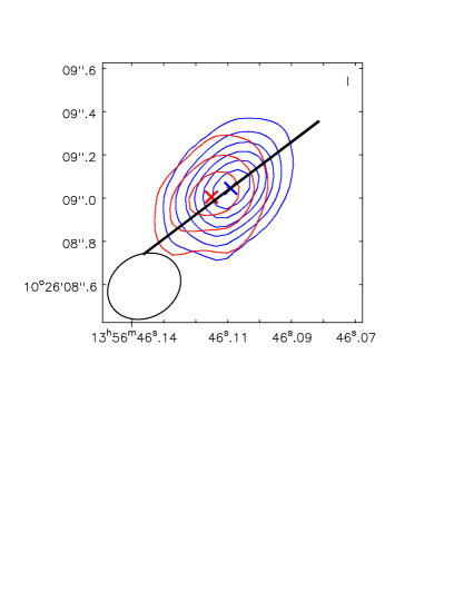
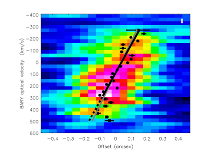
Figure 7.— Left: CO (3-2) N nucleus moment-0 map of the low velocity component $|v|<300$ km s^-1 (blue contours) and the high velocity component $v>300$ km s^-1 (red contours). The contours have a step size of 3 $\sigma$ (0.48 and 0.22 Jy beam^-1 km s^-1, respectively) between each level. The crosses show the best-fit Gaussian centroids of the two components. The beam ellipse is shown in the lower left corner. The direction of the velocity gradient of the low velocity component (P.A. $=127^{\circ}$) is indicated by the blue line. We extract a pv-diagram along this blue line and show it on the right panel. It is over a width of $0\farcs 55$, such that it contains $\sim 95\%$ of the flux. The offset on the horizontal axis is with respect to the best-fit Gaussian centroid of the low velocity component (blue cross on the left panel). The black points represents the centroid position at each velocity channel, fitted by Gaussian intensity profile. The black line shows the best-fit linear velocity gradient (1077 km s^-1 kpc^-1) of the low velocity component ($|v|<300$ km s^-1, black circles) that is consistent with a rotating disk, and the grey line is fitted to all the velocity channels ($-300<v<500$ km s^-1). The high velocity points (black squares, $v>300$ km s^-1) systematically deviate from this velocity gradient, and have velocities too high to be consistent with rotation.

5. Discussion

5.1. Origin of the Molecular Gas

We first discuss the origin and evolution of the molecular gas in the system. A significant amount of molecular gas is detected in the N nucleus and the W arm with a total mass of $9^{+19}_{-6}\times 10^{8}$ $M_{\odot}$  (Section 3). However, the stellar absorption spectrum of the N nucleus is dominated by an old stellar population (Greene et al., 2009), and based on the velocity dispersion we suspect that the galaxy started as an early-type with little cold gas. For local elliptical/S0 galaxies like SDSS J1356+1026 with $\sigma_{*}>200$ km s^-1, Young et al. (2011) find that only one out of thirty galaxies has a molecular gas mass as high as $8\times 10^{8}$ $M_{\odot}$, while most of the ellipticals are below the CO detection limit of $M_{\rm{mol}}<10^{8}$ $M_{\odot}$. Therefore, the exceptionally high molecular content in the N galaxy was likely accreted externally, perhaps from the S galaxy. The current optical spectroscopy is not adequate to identify the stellar population of the S galaxy. But if it was a late-type galaxy, with a stellar mass of about $M_{*}\approx 3\times 10^{10}$ $M_{\odot}$, it could bring in plenty of molecular gas, as the typical molecular to stellar mass ratio is about 5% for local spirals (Leroy et al., 2009; Bauermeister et al., 2013b). Gas transfer from disk companions to elliptical galaxies has been observed (Schweizer, 1987). Furthermore, some early-type galaxies have cold gas components that are kinematically decoupled from the stellar components, suggesting an external origin of the cold gas (Knapp, 1987; Davis et al., 2013). Therefore, a primary elliptical/satellite disk galaxy merger is a likely scenario to explain the molecular gas content in SDSS J1356+1026.

In simulations, when the gas collides during a merger, its orbital energy and angular momentum are dissipated, and thus the gas tunnels into the center to form a nuclear disk and triggers AGN or star formation activity (e.g., Hernquist, 1989; Barnes, 2002). In particular, if it is a primary elliptical and satellite disk galaxy merger, in some cases the gas in the disk galaxy is disrupted and sinks into the center of the primary elliptical (Weil & Hernquist, 1993). These nuclear gas disks, growing from infalling tidal tails, usually contain about half of the cool gas in the system and have peculiar kinematics relative to the stars. While these simulations do not treat the molecular gas phase explicitly, we expect the nuclear disks to have a large molecular fraction because of the dense environment. Observationally, molecular nuclear gas disks and rings are indeed common in infrared luminous mergers (Downes & Solomon, 1998). These compact nuclear disks have radii $\sim 0.5$ kpc, as opposed to $\sim 1$ kpc in normal ellipticals (Davis et al., 2013), and can be as massive as $10^{9}$ $M_{\odot}$, similar to the compact nuclear disk of SDSS J1356+1026. The energetic nuclear activity of SDSS J1356+1026 could be a direct result of the nuclear inflow induced by the interaction between the two merging galaxies (Barnes & Hernquist, 1996).

Observationally, although extended molecular tails can survive after being stripped from the galaxies (e.g., through ram pressure stripping, Dasyra et al., 2012; Jachym et al., 2014), it is not common to find a significant amount of molecular gas in tidal tails. Aalto et al. (2001) found $4\%$ ($M_{\rm{mol}}\approx 8\times 10^{7}$ $M_{\odot}$) of the molecular gas along a 10 kpc long optical tidal tail in NGC 4194, a elliptical/disk merger remnant. The ULIRG merger Mrk 273 also shows a 5 kpc extended CO streamer with mass $M_{\rm{mol}}\approx 1\times 10^{8}$ $M_{\odot}$, accounting for a few percent of the CO flux (Downes & Solomon, 1998). One of the nuclei of Mrk 273 has no molecular gas, so it was possibly a gas poor galaxy or the gas was depleted by transfer (Yun & Scoville, 1995). However, none of these examples contain as much molecular gas as in the W arm of SDSS J1356+1026 ($5\times 10^{8}$ $M_{\odot}$, half of the total molecular mass).

Both SDSS J1356+1026 and NGC 4194 are probably elliptical/disk minor mergers. We suspect that the formation of molecular tidal features may require particular progenitor properties and orbital configurations. For example, in the primary elliptical/satellite disk merger, the elliptical with its concentrated potential may disrupt the molecular disk in the satellite galaxy. At the same time, the absence of gas in the elliptical can reduce the shock dissociation of molecular gas during the encounter and thus preserve gas in the molecular phase in tidal features.

5.2. High Velocity Molecular Gas at the N Nucleus

In Section 4.1, we find a high velocity CO (3-2) feature at the N nucleus with a radius of $\sim$ 300 pc. This feature ranges in velocity from 300 to 500 km s^-1, which is too high to be part of the rotating disk. Its mass is estimated to be $M\approx 7\times 10^{7}$ $M_{\odot}$, a quarter of the mass at the N nucleus. Also, it has complex kinematics that deviate from rotation and has a slight offset with respect to the disk plane (Fig. 6, 7). There are various possible interpretations for this high velocity component. It could be inflowing or outflowing, or could result from tidal forces or feedback mechanisms. We discuss two of the most plausible scenarios.

First, the high velocity feature may represent material accreting onto the disk from an external source, perhaps the W tidal arm. The projected angular momentum of the two features are parallel to each other, although they lie on opposite sides of the disk. Furthermore, the angular momentum of the high velocity gas is smaller than the W arm, as expected for gas that is accreting onto a nuclear disk.

The second possibility is a molecular outflow. Herschel OH line observations have found molecular outflow to be a common phenomenon in ULIRG/AGN like SDSS J1356+1026 (Veilleux et al., 2013). The high velocity feature seen in SDSS J1356+1026 meets one of the outflow criterion used by the CO interferometry study by Cicone et al. (2014), in that it has a velocity above 300 km s^-1 and deviates from the rotation pattern, making it a likely outflow candidate. However, CO confirmed molecular outflows in luminous ULIRG/AGN are typically more massive and larger in size. The six molecular outflows in luminous ULIRG/AGN ($L_{\mathrm{bol}}$$>10^{44.5}$) discussed by Cicone et al. (2014), including IRAS F08572+3915, IRAS F10565+2448, IRAS 23365+3604, Mrk 273, Mrk 231, and NGC6240, have molecular outflow masses $M\approx 3\times 10^{8}$, sizes $r=$0.6-1.2 kpc, and velocities $v=$400-1200 km s^-1. This discrepancy in size could be partly due to the high angular resolution of the ALMA observations. Structures of size 300 pc may not have been resolved by previous CO studies. The fact that this compact size is measured by CO (3-2), a denser tracer than CO (1-0), may also contribute to the discrepancy. In fact, very compact molecular outflows on the scale of $\sim$100 pc have been discovered by OH observations combined with radiative-transfer modeling (Sturm et al., 2011; González-Alfonso et al., 2013).

With the current observations we are unable to completely confirm or rule out either scenario. Given the ubiquity of nuclear outflows observed with Herschel on similar scales, in what follows we elaborate further on the outflow scenario and discuss the implications of the possible compact molecular outflow in this source.

5.2.1 Properties of the Molecular Outflow

We adopt a size of $r=0.3$ kpc, velocity $v=500$ km s^-1, and mass $M\approx 7\times 10^{7}$ $M_{\odot}$ for the molecular outflow. These quantities are only order of magnitude estimates. In addition to measurement error, the size and velocity are subject to projection effects. There are also potential systematics in the mass estimate. First, the $X_{\rm{CO}}$ factor in the context of an outflow is uncertain. The lower ULIRG $X_{\rm{CO}}$ factor should already account for (at least part of) the fact that the molecular gas in outflows is not in self-gravitating clouds, but little is known about whether the violent kinematics in the outflow would further enhance the CO luminosity and thus reduce the $X_{\rm{CO}}$. In principal, if CO (1-0) became optically thin due to very turbulent velocity structure, the $X_{\rm{CO}}$ could further decrease by a factor of 2-3 (Bolatto et al., 2013). Second, we assume a typical quasar line ratio of $L^{\prime}_{\mathrm{CO(3-2)}}/L^{\prime}_{\mathrm{CO(1-0)}}=1$, but we have only a loose constraint from the observations. Potentially, the shocks in the outflow could induce a different temperature profile and thus affect the line ratio, although this effect is not seen in Mrk 231, where the excitation ratios of the molecular outflow and the bulk of the molecular gas are similar (Cicone et al., 2012).

We estimate the time scale, outflow rate, momentum, and energetics of the outflow. The dynamical time is very short, $t_{\rm{dyn}}=r/v\approx 0.6$ Myr, reflecting the compact size. The mass outflow rate depends on the geometry of the outflow, which cannot be constrained with the current data. We consider two limiting cases. If the outflow is a single burst and the material is distributed in a shell (or clump) with a distance $r$ from the center, then the mass outflow rate is $\dot{M}=Mv/r\approx 116$ $M_{\odot}$ yr^-1. If the outflow is continuous and volume filling inside a sphere or cone with a constant velocity, the mass outflow rate is $\dot{M}=3Mv/r\approx 350$ $M_{\odot}$ yr^-1, a factor of three higher due to the ratio between the surface area and the volume of a sphere. In the following we assume a volume-filling continuous outflow, as in Maiolino et al. (2012) and Cicone et al. (2014). The time it takes to deplete the molecular gas in the N nucleus ($\sim 3\times 10^{8}$ $M_{\odot}$) with a constant mass outflow rate is $t_{\rm{dep}}\approx$1 Myr. The kinetic energy and kinetic luminosity of the outflow are $E_{\rm{kin}}\approx 2\times 10^{56}$ ergs and $\dot{E}_{\rm{kin}}\approx 3\times 10^{43}$ ergs s^-1, and the momentum and momentum rate are $p\approx 7\times 10^{48}$ g cm s^-1 and $\dot{p}\approx 1\times 10^{36}$ dyne.

5.2.2 AGN or Star Formation Driven Outflow?

We now discuss the possible driving mechanism of this compact molecular outflow. To examine whether star formation can power the molecular outflow, we adopt a star formation feedback efficiency of $\dot{E}_{*}/SFR=7\times 10^{41}$ ergs s^-1 ($M_{\odot}$ yr^-1)^-1 calculated by Leitherer et al. (1999) using the stellar evolution code Starburst99 (see also Veilleux et al., 2005). The energy injection rate is dominated by supernovae that occur 40 Myr after the starburst; at earlier times the rate is lower. Therefore, to power an outflow with a kinetic luminosity of $\dot{E}\approx 3\times 10^{43}$ ergs s^-1, we need a star formation rate of at least SFR $>43$ $M_{\odot}$ yr^-1, much higher than the star formation rate that can be sustained by the molecular gas in the N nucleus (SFR $\approx 1.2$ $M_{\odot}$ yr^-1), assuming the Schmidt-Kennicutt law. It is also higher than our conservative upper-limits inferred from either the total molecular gas content (SFR $<16$ $M_{\odot}$ yr^-1 Sec. 3.3) or the far-infrared SED fitting (SFR $<21$ $M_{\odot}$ yr^-1 Sec. 3.4). To fuel a SFR of 43 $M_{\odot}$ yr^-1 in a disk of radius 300 pc requires a molecular mass of $4\times 10^{9}$ $M_{\odot}$ (Kennicutt, 1998), which is an order of magnitude higher than the molecular mass in the N nucleus and is equal to its dynamical mass. Therefore, we conclude that there is not enough star formation activity to drive the compact molecular outflow.

A jet is another possible way to drive the outflow. As discussed in Greene et al. (2012), SDSS J1356+1026 is classified as a radio-quiet quasar, and its radio emission is not resolved by the FIRST survey (beam size $5\farcs 4$, Becker et al., 1995), which puts a constraint on the size $r<2$″ (4 kpc). The agreement of flux between FIRST and NVSS, which has a larger beam size of 45″, observations suggests that there is no extended radio emission beyond the 2 ″ scale. This rules out a jet as the driver for the extended (20 kpc) ionized outflow. Our 100 GHz measurement (Sec. 3.1) further constrains the size of the high frequency radio emission to be no larger than $1\farcs 9\times 1\farcs 3$ ($4.2\times 2.9$ kpc). However, as the high frequency emission may trace only the base of the radio jet, we cannot rule out a compact jet $<2\arcsec$. Further observations are required to confirm or rule out a jet as the driving mechanism of the compact molecular outflow.

A radiative driven wind from the obscured quasar at the N nucleus (Murray et al., 1995; Proga et al., 2000) could also be responsible for driving the molecular outflow. Hydrodynamics simulations of AGN wind typically adopt a wind kinetic luminosity of a few percent of $L_{\mathrm{bol}}$ in order to reproduce the observed black hole mass - stellar velocity dispersion ($M_{\rm{BH}}-\sigma$) and the X-ray luminosity - stellar velocity dispersion ($L_{\rm{X}}-\sigma$) relations (e.g., DeBuhr et al., 2011; Choi et al., 2014). The AGN bolometric luminosity $L_{\mathrm{bol}}\approx 10^{46}$ ergs s^-1, indirectly inferred from the [O III] and mid-infrared luminosities (Sec. 3.4), is much higher than the kinetic luminosity of the molecular outflow ($\dot{E}\approx 3\times 10^{43}$ ergs s^-1) with a ratio of only $\dot{E}/L_{\mathrm{bol}}\sim 0.3\%$. The ionized outflow ($\dot{E}\approx 10^{44-45}$ ergs s^-1, Greene et al. 2012) has a kinetic luminosity $1-10\%$ of $L_{\mathrm{bol}}$. Therefore, the AGN wind is a feasible scenario in terms of energetics to drive the molecular and ionized outflows.

We find that the momentum rate ($\dot{p}\approx 1\times 10^{36}$ dyne) of the molecular outflow is similar to the radiation momentum rate from the AGN ($L_{\rm bol}/c\approx 3\times 10^{35}$ dyne) with a momentum boost of $\dot{p}/(L_{\mathrm{bol}}/c)\approx$ 3. This value is somewhat lower than what is inferred for the luminous ULIRG/AGN that have CO outflows confirmed by Cicone et al. (2014), which typically have a momentum boost of $\dot{M}v/(L_{\mathrm{bol}}/c)\mathrel{\hbox{\hbox to0.0pt{\hbox{\lower 4.0pt\hbox{$\sim$}}\hss}\hbox{\raise 2.0pt\hbox{$>$}}}}$ 20. This discrepancy may partly be due to the higher sensitivity of ALMA, which allows us to identify features of lower molecular gas mass. The lower momentum boost of the outflow in SDSS J1356+1026 indicates that it is more consistent with being momentum-driven than those found by Cicone et al. (2014). King (2003) and Zubovas & King (2012) argue that outflows on small scales tend to be momentum-conserving, because the hot wind of a luminous AGN is efficiently Compton-cooled at the vicinity of the AGN ($r\lesssim$ 1 kpc). Outflows at larger radius, in contrast, are energy-conserving. Given that the molecular outflow in SDSS J1356+1026 is more compact than other ULIRG/AGN outflows and shows a lower momentum boost, we are possibly starting to approach the momentum-driven regime of AGN outflows.

5.2.3 Comparison with the Ionized Outflow

SDSS J1356+1026 hosts an extended ionized outflow, previously discovered by Greene et al. (2012). In this section, we examine the relationship between these two outflows with their very different sizes, time scales, and molecular contents by tying them together into an integrated picture of an AGN wind interacting with galactic gas.

It is intriguing that the molecular outflow is much smaller ($r\approx 0.3$ kpc) and is characterized by shorter time scales ($t_{\rm{dyn}}\approx$ 0.6 Myr, and $t_{\rm{dep}}\approx$ 1 Myr) than the extended ionized outflow, which has $r^{\rm{ion}}\approx 10$ kpc, $v^{\rm{ion}}\approx 1000$ km s^-1, and $t^{\rm{ion}}_{\rm{dyn}}\approx 10$ Myr (Greene et al., 2012). The two outflows are different in morphology - the ionized outflow is symmetrically bipolar in the north-south direction while the compact molecular outflow has only one component which is redshifted and extends to the S-E direction. Furthermore, they have different physical conditions, as the molecular gas dominates the small scale outflow, but is ruled out as the dominant component of the extended outflow (Sec. 4.4). But the biggest puzzle is the short time scale characteristic of the molecular outflow, which raises concerns about its duty cycle: if the molecular outflow is indeed a transient phenomenon, how did we capture this rare event at this exact moment?

There are two scenarios, continuous and discrete outflows, that could account for the fact that we see outflows on very different scales. First, it could be that the quasar has been active and driving winds for more than $10^{7}$ years, and the extended ionized and compact molecular outflows are two segments of a continuous wind-driven outflow stream. They are constituted by gas of different phases possibly due to the differences in the environments, such as density. However, sustaining an outflow with a constant outflow rate of $\dot{M}=350$ $M_{\odot}$ yr^-1 for $10^{7}$ yr would require a gas mass of $\sim 10^{9.5}$ $M_{\odot}$. Unless we happened to catch the outflow in the last 10% of its life time, we would expect to find a comparable quantity of gas reservoir in the system, which we do not see. There is only $\sim 3\times 10^{8}$ $M_{\odot}$ of molecular gas at the N nucleus, which can fuel the outflow for only $\sim$ 1 Myr. Even if the molecular gas in the W arm also fuels the outflow, this outflow would only last for $\sim$ 3 Myr. There is no other gas reservoir to replenish the N nucleus; the S nucleus contains little molecular gas, and the extended outflow is unlikely to return once it travels with a velocity of 1000 km s^-1 to 10 kpc, where the escape velocity is 760 km s^-1, assuming a singular isothermal density profile with $\sigma_{*}=206$ km s^-1 (eq. 2 of Greene et al. 2011). Furthermore, we do not find $\sim 10^{9.5}$ $M_{\odot}$ of gas in the outflow, although it could be present in a hotter phase. Only $\sim 10^{7}$ $M_{\odot}$ of outflowing ionized gas is observed, although this number is only a lower limit due to the unknown gas density (Greene et al., 2011).

Discrete outflow is the second possibility. If the AGN activity is episodic (e.g., Schirmer et al., 2013; Hickox et al., 2014), the two outflows may be driven by two separate bursts of the AGN, possibly associated with multiple passages of the companion (S) galaxy. The S galaxy has an orbital period of $\sim 5\times 10^{7}$ yr, assuming a circular orbit with a radius of 2.5 kpc or free falling from a distance of 2.5 kpc. In this case, the compact molecular outflow would reflect the most recent ($\sim 10^{6}$ yr) burst while the extended ionized outflow is the relic of previous activity ($\sim 10^{7}$ yr ago). This scenario has several advantages over the continuous outflow scenario. First, we can naturally connect the time scales of the outflow to the AGN cycle, which is in the end controlled by the gas supply. Every $\sim 10^{7}$ yr, the passage of the S nucleus triggers a new burst of nuclear activity, which in turn drives a nuclear outburst that depletes the nucleus in $\sim 10^{6}$ yr, thus shutting down further activity. It is therefore not surprising to see the compact molecular outflow with both a dynamical time and a depletion time of $\sim 10^{6}$ yr. Also, it is not a coincidence that we catch this transient molecular outflow at the right time. Given that we select this object based on its bright quasar luminosity, its feedback is presumably most active. Furthermore, it could explain why we see a comparable amount of gas ($10^{7-8}$ $M_{\odot}$) in the compact and ionized outflow, if each burst releases roughly the same amount of energy and expels the same amounts of gas. An outflow driven by episodic AGN activity seems to be a reasonable possibility that is consistent with the various measured time and mass scales.

6. Summary

The sub-millimeter observations of CO (1-0) and CO (3-2) with ALMA of the luminous obscured quasar SDSS J1356+1026 provide insights into molecular gas dynamics during a merger, AGN feedback on molecular gas, and episodic AGN activity on 10 Myr time scales. We summarize the highlights of our study below.

SDSS J1356+1026 contains two merging nuclei, with the primary galaxy likely of early type. Given the high molecular content we find in the system ($M_{\rm{mol}}\approx 9^{+19}_{-6}\times 10^{8}$ $M_{\odot}$), we speculate that the secondary galaxy was a disk galaxy which brought in the majority of the gas. In this scenario, the cold gas from the secondary was disrupted during the encounter. Roughly a third of the gas sank into the primary nucleus and formed a compact disk (N nucleus, $r\approx 300$ pc, $M_{\rm{mol}}\approx 3^{+6}_{-2}\times 10^{8}$ $M_{\odot}$), while half of the gas is now in an extended tidal tail (W arm, $r\approx$ 5 kpc, $M_{\rm{mol}}\approx 5^{+11}_{-3}\times 10^{8}$ $M_{\odot}$), which is one of the most massive molecular tidal features known.

In addition to a compact disk, we find a red-shifted high-velocity component deviating from rotation at the N nucleus. It has a compact size of $\sim 300$ pc and a velocity of $\sim 500$ km s^-1. Although the origin of this gas is not clear, we suspect it is an outflow driven by the AGN. Our estimated star formation rate limits, SFR $<16$ $M_{\odot}$ yr^-1 from the CO molecular content and SFR $<21$ $M_{\odot}$ yr^-1 from the FIR SED decomposition, disfavor star formation as the driving mechanism. A molecular outflow with $\dot{M}\approx 350$ $M_{\odot}$ yr^-1 could expel all gas in the N nucleus in $\sim$ 1 Myr and all the molecular gas in the system in $\sim$ 3 Myr. It is one of the most compact CO molecular outflows discovered, and the corresponding dynamical time is short $\sim 0.6$ Myr. The kinetic luminosity of this outflow $\dot{E}\approx 3\times 10^{43}$ ergs s^-1 is only $\sim 0.3\%$ of the AGN bolometric luminosity $L_{\mathrm{bol}}\approx 10^{46}$ ergs s^-1. Its low momentum boost rate $\dot{p}/(L_{\mathrm{bol}}/c)\approx$ 3 is consistent with the prediction that compact AGN outflows tend to be momentum conserving (Zubovas & King, 2012). The compact molecular outflow discovered here and the extended ionized outflow (Greene et al., 2012) are likely induced from two episodes of AGN activity, varying on a time scale of $10$ Myr.

SDSS J1356+1026 is an example of a molecular outflow that can effectively disturb or deplete the molecular reservoir in the galaxy. Molecular outflows identified by high velocity OH absorption features are found to be common among AGN (Sturm et al., 2011; Veilleux et al., 2013). As demonstrated in this work, spatially resolved CO observations provide a complementary and model independent technique to measure the size and mass, and to infer the mass-lost rate of the outflow ($\dot{M}$). In the end, whether AGN feedback is a successful model to account for the absence of luminous blue galaxies and the cut-off of the galaxy luminosity function depends on both the frequency and the mass-lost rate of molecular outflows as a function of AGN luminosity. Furthermore, both molecular and ionized outflows are found to be ubiquitous in luminous quasars (Liu et al., 2013a, b; Harrison et al., 2014), and can coexist (Davis et al., 2012; Rupke & Veilleux, 2013), but we do not fully understand how they are related. Also, the connection between the compactness and the low momentum boost rate of molecular outflows, as hinted by SDSS J1356+1026, requires confirmation from a larger spatially resolved sample. These outstanding questions could be answered with systematic and spatially resolved observations of molecular gas in a sample of AGN covering a range of luminosities and ionized outflow properties. As demonstrated in this work, with its great sensitivity and resolution, ALMA is well suited for resolving molecular outflows on sub-kpc scales to as far as $z=0.1$, and is therefore a powerful tool to bring our understanding of AGN feedback to the next level.

Acknowledgements: We thank the referee for the useful comments and Andreea Petric and Luis Ho for kindly providing the Herschel photometry. A. Sun is thankful for Brandon Hensley, Jerry Ostriker, Jim Gunn, Paul Ho, Hauyu Baobab Liu, Satoki Matsushita, Sylvain Veilleux, Timothy Davis, and Joan Wrobel for constructive discussions. A. Sun was partially supported by the NRAO Student Observing Support grant SOSPA0-013.

This paper makes use of the following ALMA data: ADS/JAO.ALMA#2011.0.00652.S and 2012.1.00797.S. ALMA is a partnership of ESO (representing its member states), NSF (USA) and NINS (Japan), together with NRC (Canada) and NSC and ASIAA (Taiwan), in cooperation with the Republic of Chile. The Joint ALMA Observatory is operated by ESO, AUI/NRAO and NAOJ. The National Radio Astronomy Observatory is a facility of the National Science Foundation operated under cooperative agreement by Associated Universities, Inc. This publication makes use of data products from the Wide-field Infrared Survey Explorer, which is a joint project of the University of California, Los Angeles, and the Jet Propulsion Laboratory/California Institute of Technology, funded by the National Aeronautics and Space Administration. Herschel is an ESA space observatory with science instruments provided by European-led Principal Investigator consortia and with important participation from NASA.

References

- Aalto et al. (2012) Aalto, S., Garcia-Burillo, S., Muller, S., et al. 2012, Astronomy and Astrophysics, 537, A44
- Aalto et al. (2001) Aalto, S., H ttemeister, S., & Polatidis, A. G. 2001, Astronomy and Astrophysics, 372, L29
- Abazajian et al. (2009) Abazajian, K. N., Adelman-McCarthy, J. K., Agüeros, M. A., et al. 2009, The Astrophysical Journal Supplement Series, 182, 543
- Alatalo et al. (2011) Alatalo, K., Blitz, L., Davis, T. A., et al. 2011, The Astrophysical Journal, 735, 88
- Barnes (2002) Barnes, J. E. 2002, Monthly Notices of the Royal Astronomical Society, 333, 481
- Barnes & Hernquist (1996) Barnes, J. E., & Hernquist, L. 1996, The Astrophysical Journal, 471, 115
- Bauermeister et al. (2013a) Bauermeister, A., Blitz, L., Bolatto, A., et al. 2013a, The Astrophysical Journal, 763, 64
- Bauermeister et al. (2013b) —. 2013b, The Astrophysical Journal, 768, 132
- Becker et al. (1995) Becker, R. H., White, R. L., & Helfand, D. J. 1995, The Astrophysical Journal, 450, 559
- Bell (2003) Bell, E. F. 2003, The Astrophysical Journal, 586, 794
- Bolatto et al. (2013) Bolatto, A. D., Wolfire, M., & Leroy, A. K. 2013, Annual Review of Astronomy and Astrophysics
- Booth & Schaye (2010) Booth, C. M., & Schaye, J. 2010, MNRAS, 405, L1
- Bower et al. (2006) Bower, R. G., Benson, A. J., Malbon, R., et al. 2006, Monthly Notices of the Royal Astronomical Society, 370, 645
- Briggs (1995) Briggs, D. S. 1995, Bulletin of the American Astronomical Society, 27, 1444
- Bruzual & Charlot (2003) Bruzual, G., & Charlot, S. 2003, Monthly Notices of the Royal Astronomical Society, 344, 1000
- Carilli & Walter (2013) Carilli, C. L., & Walter, F. 2013, Annual Review of Astronomy and Astrophysics, 51, 105
- Choi et al. (2014) Choi, E., Naab, T., Ostriker, J. P., Johansson, P. H., & Moster, B. P. 2014, Monthly Notices of the Royal Astronomical Society, 442, 440
- Cicone et al. (2012) Cicone, C., Feruglio, C., Maiolino, R., et al. 2012, Astronomy and Astrophysics, 543, A99
- Cicone et al. (2014) Cicone, C., Maiolino, R., Sturm, E., et al. 2014, Astronomy and Astrophysics, 562, A21
- Ciotti & Ostriker (2001) Ciotti, L., & Ostriker, J. P. 2001, ApJ, 551, 131
- Condon et al. (1998) Condon, J. J., Cotton, W. D., Greisen, E. W., et al. 1998, The Astronomical Journal, 115, 1693
- Croton et al. (2006) Croton, D. J., Springel, V., White, S. D. M., et al. 2006, Monthly Notices of the Royal Astronomical Society, 365, 11
- Dasyra et al. (2012) Dasyra, K. M., Combes, F., Salomé, P., & Braine, J. 2012, Astronomy and Astrophysics, 540, A112
- Davis et al. (2012) Davis, T. A., Krajnović, D., McDermid, R. M., et al. 2012, Monthly Notices of the Royal Astronomical Society, 426, 1574
- Davis et al. (2013) Davis, T. A., Alatalo, K., Bureau, M., et al. 2013, Monthly Notices of the Royal Astronomical Society, 429, 534
- DeBuhr et al. (2011) DeBuhr, J., Quataert, E., & Ma, C.-P. 2011, Monthly Notices of the Royal Astronomical Society, 420, 2221
- Downes & Solomon (1998) Downes, D., & Solomon, P. M. 1998, The Astrophysical Journal, 507, 615
- Fabian (2012) Fabian, A. C. 2012, Annual Review of Astronomy and Astrophysics, 50, 455
- Faucher-Giguère & Quataert (2012) Faucher-Giguère, C.-A., & Quataert, E. 2012, Monthly Notices of the Royal Astronomical Society, 425, 605
- Feruglio et al. (2010) Feruglio, C., Maiolino, R., Piconcelli, E., et al. 2010, Astronomy and Astrophysics, 518, L155
- Feruglio et al. (2012) Feruglio, C., Fiore, F., Maiolino, R., et al. 2012, Astronomy and Astrophysics, 549, 99051
- Flower & Pineau des Forets (2013) Flower, D. R., & Pineau des Forets, G. 2013, Monthly Notices of the Royal Astronomical Society, 436, 2143
- Fu & Stockton (2008) Fu, H., & Stockton, A. 2008, The Astrophysical Journal, 690, 953
- González-Alfonso et al. (2013) González-Alfonso, E., Fischer, J., Graciá-Carpio, J., et al. 2013, Astronomy and Astrophysics, 561, A27
- Greene et al. (2014) Greene, J. E., Pooley, D., Zakamska, N. L., Comerford, J. M., & Sun, A.-L. 2014, The Astrophysical Journal, 788, 54
- Greene et al. (2011) Greene, J. E., Zakamska, N. L., Ho, L. C., & Barth, A. J. 2011, The Astrophysical Journal, 732, 9
- Greene et al. (2009) Greene, J. E., Zakamska, N. L., Liu, X., Barth, A. J., & Ho, L. C. 2009, The Astrophysical Journal, 702, 441
- Greene et al. (2012) Greene, J. E., Zakamska, N. L., & Smith, P. S. 2012, The Astrophysical Journal, 746, 86
- Griffin et al. (2010) Griffin, M. J., Abergel, A., Abreu, A., et al. 2010, Astronomy and Astrophysics, 518, L3
- Hainline et al. (2013) Hainline, K. N., Hickox, R., Greene, J. E., Myers, A. D., & Zakamska, N. L. 2013, The Astrophysical Journal, 774, 145
- Harrison et al. (2014) Harrison, C. M., Alexander, D. M., Mullaney, J. R., & Swinbank, A. M. 2014, MNRAS accepted (arXiv:1403.3086)
- Hernquist (1989) Hernquist, L. 1989, Nature, 340, 687
- Hibbard et al. (2000) Hibbard, J. E., Vacca, W. D., & Yun, M. S. 2000, The Astronomical Journal, 119, 1130
- Hickox et al. (2014) Hickox, R. C., Mullaney, J. R., Alexander, D. M., et al. 2014, The Astrophysical Journal, 782, 9
- Hyde & Bernardi (2009) Hyde, J. B., & Bernardi, M. 2009, Monthly Notices of the Royal Astronomical Society, 394, 1978
- Jachym et al. (2014) Jachym, P., Combes, F., Cortese, L., Sun, M., & Kenney, J. D. P. 2014, ApJ submitted (arXiv:1403.2328)
- Kennicutt (1998) Kennicutt, Jr, R. C. 1998, The Astrophysical Journal, 498, 541
- King (2003) King, A. 2003, The Astrophysical Journal, 596, L27
- Kirkpatrick et al. (2012) Kirkpatrick, A., Pope, A., Alexander, D. M., et al. 2012, The Astrophysical Journal, 759, 139
- Knapp (1987) Knapp, G. R. 1987, Structure and Dynamics of Elliptical Galaxies, 127, 145
- Kormendy & Ho (2013) Kormendy, J., & Ho, L. C. 2013, Annual Review of Astronomy and Astrophysics, 51, 511
- Leitherer et al. (1999) Leitherer, C., Schaerer, D., Goldader, J. D., et al. 1999, The Astrophysical Journal Supplement Series, 123, 3
- Leroy et al. (2009) Leroy, A. K., Walter, F., Bigiel, F., et al. 2009, AJ, 137, 4670
- Liu et al. (2013a) Liu, G., Zakamska, N. L., Greene, J. E., Nesvadba, N. P. H., & Liu, X. 2013a, Monthly Notices of the Royal Astronomical Society, 430, 2327
- Liu et al. (2013b) —. 2013b, Monthly Notices of the Royal Astronomical Society, 436, 2576
- Liu et al. (2009) Liu, X., Zakamska, N. L., Greene, J. E., et al. 2009, The Astrophysical Journal, 702, 1098
- Maiolino et al. (2012) Maiolino, R., Gallerani, S., Neri, R., et al. 2012, Monthly Notices of the Royal Astronomical Society: Letters, 425, L66
- McConnell & Ma (2013) McConnell, N. J., & Ma, C.-P. 2013, The Astrophysical Journal, 764, 184
- Murray et al. (1995) Murray, N., Chiang, J., Grossman, S. A., & Voit, G. M. 1995, ApJ, 451, 498
- Nesvadba et al. (2006) Nesvadba, N. P. H., Lehnert, M. D., Eisenhauer, F., et al. 2006, The Astrophysical Journal, 650, 693
- Neugebauer et al. (1984) Neugebauer, G., Habing, H. J., van Duinen, R., et al. 1984, The Astrophysical Journal, 278, L1
- Page et al. (2012) Page, M. J., Symeonidis, M., Vieira, J. D., et al. 2012, Nature, 485, 213
- Pilbratt et al. (2010) Pilbratt, G. L., Riedinger, J. R., Passvogel, T., et al. 2010, Astronomy and Astrophysics, 518, L1
- Poglitsch et al. (2010) Poglitsch, A., Waelkens, C., Geis, N., et al. 2010, Astronomy and Astrophysics, 518, L2
- Proga et al. (2000) Proga, D., Stone, J. M., & Kallman, T. R. 2000, The Astrophysical Journal, 543, 686
- Richards et al. (2006) Richards, G. T., Lacy, M., Storrie Lombardi, L. J., et al. 2006, The Astrophysical Journal Supplement Series, 166, 470
- Rupke et al. (2005) Rupke, D. S., Veilleux, S., & Sanders, D. B. 2005, The Astrophysical Journal, 632, 751
- Rupke & Veilleux (2013) Rupke, D. S. N., & Veilleux, S. 2013, The Astrophysical Journal, 768, 75
- Schirmer et al. (2013) Schirmer, M., Diaz, R., Holhjem, K., Levenson, N. A., & Winge, C. 2013, The Astrophysical Journal, 763, 60
- Schweizer (1987) Schweizer, F. 1987, Structure and Dynamics of Elliptical Galaxies, 127, 109
- Skrutskie et al. (2006) Skrutskie, M. F., Cutri, R. M., Stiening, R., et al. 2006, AJ, 131, 1163
- Solomon et al. (1987) Solomon, P. M., Rivolo, A. R., Barrett, J., & Yahil, A. 1987, The Astrophysical Journal, 319, 730
- Stockton & MacKenty (1987) Stockton, A., & MacKenty, J. W. 1987, The Astrophysical Journal, 316, 584
- Sturm et al. (2011) Sturm, E., González-Alfonso, E., Veilleux, S., et al. 2011, The Astrophysical Journal, 733, L16
- Sun et al. (2013) Sun, A.-L., Greene, J. E., Impellizzeri, C. M. V., et al. 2013, The Astrophysical Journal, 778, 47
- Teng et al. (2013) Teng, S. H., Veilleux, S., & Baker, A. J. 2013, The Astrophysical Journal, 765, 95
- Veilleux et al. (2005) Veilleux, S., Cecil, G., & Bland-Hawthorn, J. 2005, Annual Review of Astronomy and Astrophysics, 43, 769
- Veilleux et al. (2013) Veilleux, S., Meléndez, M., Sturm, E., et al. 2013, The Astrophysical Journal, 776, 27
- Villar-Martin et al. (2014) Villar-Martin, M., Emonts, B., Humphrey, A., Cabrera Lavers, A., & Binette, L. 2014, Monthly Notices of the Royal Astronomical Society, 440, 3202
- Villar-Martin et al. (2011) Villar-Martin, M., Humphrey, A., Delgado, R. G., Colina, L., & Arribas, S. 2011, Monthly Notices of the Royal Astronomical Society, 418, 2032
- Walter et al. (2002) Walter, F., Weiss, A., & Scoville, N. 2002, The Astrophysical Journal, 580, L21
- Wang et al. (2011) Wang, J., Fabbiano, G., Elvis, M., et al. 2011, The Astrophysical Journal, 736, 62
- Wang et al. (2009) Wang, J., Fabbiano, G., Karovska, M., et al. 2009, The Astrophysical Journal, 704, 1195
- Weil & Hernquist (1993) Weil, M. L., & Hernquist, L. 1993, The Astrophysical Journal, 405, 142
- Whittle (1992) Whittle, M. 1992, The Astrophysical Journal, 387, 109
- Wright et al. (2010) Wright, E. L., Eisenhardt, P. R. M., Mainzer, A. K., et al. 2010, AJ, 140, 1868
- Young et al. (2011) Young, L. M., Bureau, M., Davis, T. A., et al. 2011, Monthly Notices of the Royal Astronomical Society, 414, 940
- Yuma et al. (2013) Yuma, S., Ouchi, M., Drake, A. B., et al. 2013, The Astrophysical Journal, 779, 53
- Yun & Scoville (1995) Yun, M. S., & Scoville, N. Z. 1995, The Astrophysical Journal, 451
- Zakamska & Greene (2014) Zakamska, N. L., & Greene, J. E. 2014, MNRAS accepted (arXiv:1402.6736)
- Zakamska et al. (2004) Zakamska, N. L., Strauss, M. A., Heckman, T. M., Ivezić, Ž., & Krolik, J. H. 2004, AJ, 128, 1002
- Zubovas & King (2012) Zubovas, K., & King, A. 2012, The Astrophysical Journal, 745, L34