An Algorithm to classify rational 3-tangles

Abstract.

A $3$-$tangle$ $T$ is the disjoint union of $3$ properly embedded arcs in the unit 3-ball; it is called rational if there is a homeomorphism of pairs from $(B^{3},T)$ to $(D^{2}\times I,\{x_{1},x_{2},x_{3}\}\times I)$. Two rational 3-tangles $T$ and $T^{\prime}$ are isotopic if there is an orientation-preserving self-homeomorphism $h:(B^{3},T)\rightarrow(B^{3},T^{\prime})$ that is the identity map on the boundary. In this paper, we give an algorithm to check whether or not two rational 3-tangles are isotopic by using a modified version of Dehn’s method for classifying simple closed curves on surfaces.

1. Introduction

Tangles were introduced by J. Conway. In 1970, he proved that every rational 2-tangle defines a rational number and two rational 2-tangles are isotopic if and only if they have the same rational number. However, there is no similar invariant known which classifies rational $3$-tangles. In this paper, I describe an algorithm to check whether or not two rational $3$-tangles are isotopic.

A n-tangle is the disjoint union of $n$ properly embedded arcs in the unit 3-ball; the embedding must send the endpoints of the arcs to $2n$ marked (fixed) points on the ball’s boundary. Without loss of generality, consider the marked points on the 3-ball boundary to lie on a great circle. The tangle can be arranged to be in general position with respect to the projection onto the flat disk in the $xy$-plane bounded by the great circle. The projection then gives us a tangle diagram, where we make note of over and undercrossings as with knot diagrams. A $rational$ $n$-$tangle$ is a $n$-tangle $\alpha_{1}\cup\alpha_{2}\cup\cdot\cdot\cdot\cup\alpha_{n}$ in a 3-ball $B^{3}$ such that there exists a homeomorphism of pairs $\overline{H}:(B^{3},\alpha_{1}\cup\alpha_{2}\cup\cdot\cdot\cdot\cup\alpha_{n})\longrightarrow(D^{2}\times I,\{p_{1},p_{2},\cdot\cdot\cdot,p_{n}\}\times I)$, where $I=[0,1]$.

We note that there exists a homeomorphism $K:(D^{2}\times I,\{p_{1},p_{2},\cdot\cdot\cdot,p_{n}\}\times I)\rightarrow(B^{3},\epsilon_{1}\cup\epsilon_{2}\cup\cdot\cdot\cdot\cup\epsilon_{n})$, where $\epsilon_{1}\cup\epsilon_{2}\cup\cdot\cdot\cdot\cup\epsilon_{n}$ is the $\infty$ tangle as in Figure 1.

Therefore, alternatively, a $n$-tangle $\alpha_{1}\cup\alpha_{2}\cup\cdot\cdot\cdot\cup\alpha_{n}$ is rational if there exists a homeomorphism of pairs: $\widehat{H}=(\overline{H})^{-1}K^{-1}:(B^{3},\epsilon_{1}\cup\epsilon_{2}\cup\cdot\cdot\cdot\cup\epsilon_{n})\rightarrow(B^{3},\alpha_{1}\cup\alpha_{2}\cup\cdot\cdot\cdot\cup\alpha_{n})$.

Two rational $n$-tangles, $T,T^{\prime}$, in $B^{3}$ are isotopic, denoted by $T\approx T^{\prime}$, if there is an orientation-preserving self-homeomorphism $h:(B^{3},T)\rightarrow(B^{3},T^{\prime})$ that is the identity map on the boundary.

Figure 1. Examples of rational 3-tangles

Let $\Sigma_{0,6}$ be the six punctured sphere and let $\epsilon=\epsilon_{1}\cup\epsilon_{2}\cup\epsilon_{3}$ be the $\infty$ 3-tangle as in Figure 2. Then, for two orientation preserving homeomorphisms $f$ and $g$ from $\Sigma_{0,n}$ to $\Sigma_{0,n}$, we say they are isotopic, denoted by $f\sim g$, if there is a continuous map $H:\Sigma_{0,n}\times I\rightarrow\Sigma_{0,n}$ so that $H(x,1)=f(x)$ and $H(x,0)=g(x)$ and $h_{t}(x)=H(x,t)$ is a homeomorphism for all $t$. Also, we say that a subset $C_{1}$ of $\Sigma_{0,n}$ is isotopic to $C_{2}$, denoted by $C_{1}\sim C_{2}$, if there is a homeomorphism $h$ of $\Sigma_{0,6}$ with $h(C_{1})=C_{2}$ such that $h\sim id$.

To demonstrate the effectiveness of this algorithm, we will show that the rational $3$-tangles in Figure 1 are not isotopic to each other. Note that for every string of $T$, if we consider the other two strings then they are isotopic to a trivial rational 2-tangle in $B^{3}$. However, we will show that $T$ is not isotopic to the $\infty$ tangle. So, $T$ is similar to the Borromean rings. We will also show that $T$ is not isotopic to the tangle $T^{\prime}$ which is obtained from $T$ by reversing all the crossings in $T$.

The algorithm is based on the following facts, which are proved in Section 2.

Up to isotopy, orientation preserving homeomorphisms $f$ and $g$ from $\Sigma_{0,6}$ to $\Sigma_{0,6}$ which fix the puncture 1 can be obtained by four half Dehn twists $\sigma_{1},\sigma_{2},\sigma_{3}$ and $\sigma_{4}$ which are the generators of the braid group $\mathbb{B}_{5}$. (Refer to [2].)

Then we can get extensions $F,G:B^{3}\rightarrow B^{3}$ of $f$ and $g$ which fix the set of six points, $\epsilon\cap\partial B^{3}$, setwise giving two rational 3-tangles $T_{F}:=F({\epsilon})$ and $T_{G}:=G({\epsilon})$.

We will show that a tangle can be “presented” by an element of $\mathbb{B}_{5}$ and our algorithm will decide whether or not two elements of $\mathbb{B}_{5}$ present equivalent tangles. We will discuss this in Section 2.

We say that a disk $D$ is essential in $B^{3}-T$ for a rational 3-tangle $T$ if $D$ is a properly embedded disk in $B^{3}-T$ but it is not boundary parallel in $B^{3}-T$.

Figure 2. A trivial rational 3-tangle, $\epsilon$

$\bf{Theorem~{}2.3}$ For two rational 3-tangles $T_{F}$ and $T_{G}$, $T_{F}\approx T_{G}$ if and only if $G^{-1}F(\partial E)$ bounds essential disks in $B^{3}-\epsilon$, where $E=E_{1}\cup E_{2}\cup E_{3}$ is a fixed union of “standard essential disks” in $B^{3}-\epsilon$. (Refer to Figure 2.)

In fact, if $G^{-1}F(\partial E_{i})$ and $G^{-1}F(\partial E_{j})$ bound essential disks in $B^{3}-\epsilon$ then $G^{-1}F(\partial E_{k})$ also bounds an essential disk in $B^{3}-\epsilon$ for $\{i,j,k\}=\{1,2,3\}$. Therefore, if two of $G^{-1}F(\partial E)$ bound essential disks then $T_{F}\approx T_{G}$.

We note that there is another way to check whether $G^{-1}F(\partial E_{i})$ bounds an essential disk in $B^{3}-\epsilon$ or not by using a fundamental group argument. There is an induced map $i_{*}:\pi_{1}(\Sigma_{0,6})\rightarrow\pi_{1}(B^{3}-\epsilon)$ from the inclusion map $i:\Sigma_{0,6}\rightarrow B^{3}-\epsilon$. Then we know that if $i_{*}([G^{-1}F(\partial E_{i})])=1$ then $G^{-1}F(\partial E_{i})$ bounds an essential disk in $B^{3}-\epsilon$ by Dehn’s Lemma. This method is conceptually simple but it appears to be awkward to implement due to having to deal with arbitrarily long words in a free group. However, if one uses the algorithm given below to check whether or not $G^{-1}F(\partial E_{i})$ bounds an essential disk in $B^{3}-\epsilon$ then we will be dealing with integer vectors of fixed dimension. I will give an example to compare the two algorithms later.

Let $\mathcal{C}$ be the set of isotopy classes of closed essential simple closed curves in $\Sigma_{0,6}$. A simple closed curve $\gamma$ is essential in $\Sigma_{0,6}$ if $\gamma$ does not bound a disk in $\Sigma_{0,6}$ and $\gamma$ does not enclose a single puncture of $\Sigma_{0,6}$.

The algorithm is as follows:

Step 1: We represent $\Sigma_{0,6}$ as the union of two hexagons $H$ and $H^{c}$ so that the vertices are the punctures of $\Sigma_{0,6}$. Then we use a variation of normal curve theory to parameterize $\mathcal{C}$. Each curve has a “hexagon diagram”. A set of “weights” $w_{ij}$ and $w^{kl}$ for the hexagon diagram parameterizes the set of isotopy classes $[G^{-1}F(\partial E_{s})]$. Using certain formulas the weights can be obtained easily from the words in $\sigma_{1},\cdot\cdot\cdot,\sigma_{4}$ which describe $F$ and $G$, but the weights are hard to use directly to decide whether or not $G^{-1}F(\partial E_{s})$ bounds an essential disk.

Step 2: We find a simple closed curve $\gamma^{\prime}$, possibly not isotopic to $\gamma$, which bounds an essential disk in $B^{3}-\epsilon$ if and only if the component $\gamma$ of $G^{-1}F(\partial E_{i})$ does. We take a decomposition of $\Sigma_{0,6}$ into three $2$-punctured disks $E_{i}^{\prime}$ and one pair of pants $I$, where each $2$-punctured disk contains one component of $H\cap H^{c}$. We specify the isotopy class $[\gamma^{\prime}]$ by using a modified version of Dehn’s method. (See [5].) We define the Dehn parameters $p_{i},q_{i}$ and $t_{i}$ ($1\leq i\leq 3$) of $[\gamma^{\prime}]$ in $E_{i}^{\prime}$ and the weights $x_{jk}$ ($1\leq j,k\leq 3$) of $[\gamma^{\prime}]$ in $I$. The $x_{jk}$ are determined by $p_{i},q_{i}$ and $t_{i}$. We note that the Dehn parameters $p_{i},q_{i}$ and $t_{i}$ ($1\leq i\leq 3$) of $[\gamma^{\prime}]$ are obtained from the weights $w_{ij}$ and $w^{kl}$ for the hexagon diagram, where $i,j,k,l\in\{1,2,3,4,5,6\}$.

Step 3: We modify $\gamma^{\prime}$ into $\gamma_{0}$, possibly not isotopic to $\gamma^{\prime}$ or $\gamma$, which is in “standard position” and bounds an essential disk in $B^{3}-\epsilon$ if and only if $\gamma^{\prime}$ does. Then we get “standard weights” $m_{i}\geq 0$ ($1\leq i\leq 11$) of $\gamma_{0}$ from the Dehn parameters. Standard position is slightly reminiscent of train track theory, but involves fewer diagrams.

Step 4: We define three homeomorphisms $\delta_{1},\delta_{2}$ and $\delta_{3}$ so that $\gamma_{0}$ bounds an essential disk in $B^{3}-\epsilon$ if and only if both $\delta_{1}\delta_{2}^{-1}(\gamma_{0})$ and $\delta_{3}(\gamma_{0})$ bound essential disks in $B^{3}-\epsilon$. Then, we repeatedly apply Theorem 9.3 below to check whether $\gamma_{0}$ bounds an essential disk in $B^{3}-\epsilon$, where $I^{\prime}$ is certain regular heighborhood of $I$.

$\mathbb{Theorem~{}\ref{T93}}$ Suppose that $\gamma_{0}$ bounds an essential disk in $B^{3}-\epsilon$ and $\gamma_{0}$ is in standard position in $I^{\prime}$ and $m_{3}>0$. Then applying one of the homeomorphisms $(\delta_{1}\delta_{2}^{-1})^{\pm 1}$ and $\delta_{3}^{\pm 1}$ reduces the sum of the $p_{i}$ for the image of $\gamma_{0}$.

Suppose that a simple closed curve $\gamma_{0}$ is in standard position and has $m_{3}>0$. If we can reduce the sum of the standard weights of $\gamma_{0}$ by using one of the four homeomorphisms then we take the new simple closed curve $\gamma_{1}$ which is obtained by applying one of the four homeomorphisms. If not, then $\gamma_{0}$ does not bound an essential disk. If $\gamma_{1}$ still has $m_{3}>0$, then we will go on. Suppose $m_{3}=0$. Then $\gamma_{1}$ is isotopic to one of the $\partial E_{k}$ if $m_{i}=0$ for all $i$. It does not bound an essential disk in $B^{3}-\epsilon$ if $m_{i}\neq 0$ for some $i$. Since the sum of the standard weights is finite, the algorithm will end in a finite number of steps.

Recall that $\gamma_{0}$ bounds an essential disk in $B^{3}-\epsilon$ if and only if $G^{-1}F(\partial E_{i})$ does. So, the given procedures form an algorithm to classify rational 3-tangles.

The author would like to thank his advisor Robert Myers for his consistent encouragement and sharing his enlightening ideas on the foundations of this topic.

2. Presentations of rational 3-tangles

We recall that a rational 3-tangle $T$ can be arranged to be in general position with respect to the projection onto the flat disk $Q$ in the $xy$-plane bounded by the great circle $C$. Then we will have a tangle diagram $TD$ of the rational 3-tangle $T$. Let $p$ be the number of crossings of the tangle $T$ in the diagram.

Figure 3. A standard diagram of a rational 3-tangle expressed by $w=\tau_{5}^{-1}\tau_{4}^{-1}\tau_{3}\tau_{2}\tau_{1}$.

Now, we say that a tangle diagram $TD$ is standard if for the nested disks $Q_{1}\subset Q_{2}\subset\cdot\cdot\cdot\subset Q_{p+1}$, $Q_{1}$ contains the $\infty$ tangle and each annulus $N_{j}=Q_{j+1}-Q_{j}^{\circ}$ contains exactly one crossing of the crossings of $T$ as in Figure 3.

Then we define a rational 3-tangle $T$ to be in standard position if the projection of $T$ onto the flat disk in the $xy$-plane bounded by $C$ is a standard diagram.

Let $\sigma_{i}$ be the half Dehn twist supported on the twice punctured disk $K_{i}$ as in Figure 4.

Figure 4. Generators of the mapping class group of $\Sigma_{0,6}$

Then we have an extension $\tau_{i}$ of $\sigma_{i}$ to $B^{3}$ as follows.

Figure 5. The extension $\tau_{i}$ of a half Dehn twist $\sigma_{i}$ to $B^{3}$

Take a ball $B_{i}$ in $B^{3}$ so that $B_{i}\cap\partial B^{3}=\overline{K_{i}}$ and $B_{i}\cap\epsilon$ is two trivial subarcs of $\epsilon$ as in Figure 5.

Then, we define $\tau_{i}$ so that $\tau_{i}|_{B^{3}-B_{i}}=id$ and $\tau_{i}|_{B_{i}}$ is an extension of $\sigma_{i}$ to $B_{i}$ which twists the two trivial simple subarcs in $B_{i}$ to have a positive crossing as in Figure 5.

Lemma 2.1.

Suppose that $F$ is an orientation preserving homeomorphism from $B^{3}$ to $B^{3}$ so that $F(\{1,2,3,4,5,6\})=\{1,2,3,4,5,6\}$. Then, there exists an orientation preserving homeomorphism $F_{1}:B^{3}\rightarrow B^{3}$ so that $F_{1}(1)=1$ and $F_{1}(\epsilon)=F(\epsilon)$.

Proof.

First, we claim that there is a homeomorphism $R_{i}:(B^{3},\epsilon)\rightarrow(B^{3},\epsilon)$ so that $R_{i}(1)=i$ for $i\in\{1,2,3,4,5,6\}$.

We note that there is a homeomorphism $\rho_{j}:(B^{3},\epsilon)\rightarrow(B^{3},\epsilon)$ so that $\rho_{j}(1)=j$ for $j=1,3$ or $5$ by using $0^{\circ}$, $120^{\circ}$ or $240^{\circ}$ counterclockwise rotation in the plane. Then we remark that it preserves $\epsilon$ setwise. So, $R_{i}=\rho_{i}$ for $i=1,3,5$.

We note that $\tau_{k}$ switches the two endpoints of $\epsilon_{1+{k\over 2}}$ for $k=0,2,4$.

We let $R_{i}:(B^{3},\epsilon)\rightarrow(B^{3},\epsilon)$ be $R_{i}=\tau_{i-2}\circ\rho_{i-1}$ for $i=2,4,6$. We check that $R_{i}(1)=i$ for $i=2,4,6$.

Suppose that $F(p)=1$. Then we let $F_{1}=F\circ R_{p}$. So, we have $F_{1}(1)=F(R_{p}(1))=F(p)=1$. Also, we know that $F_{1}(\epsilon)=F(R_{p}(\epsilon))=F(\epsilon)$ since $R_{p}(\epsilon)=\epsilon$.

∎

Now, by Lemma 2.1, we may assume $F(1)=1$. This will be assumed throughtout the rest of the paper.

Let $f=F|_{\Sigma_{0,6}}$. Then it is an orientation preserving homeomorphism from $\Sigma_{0,6}$ to $\Sigma_{0,6}.$ The mapping class group of $\Sigma_{0,6}$ is $\mathcal{MCG}(\Sigma_{0,6})=Homeo^{+}(\Sigma_{0,6})/\sim$.

Let $\mathcal{MCG}_{1}(\Sigma_{0,6})=\{[h]\in\mathcal{MCG}(\Sigma_{0,6})~{}|~{}h(1)=1\}$, where $[h]$ is the isotopy class of $h$. Then, $[f]\in\mathcal{MCG}_{1}(\Sigma_{0,6})$.

Recall the two rational 3-tangles $T$ and $T^{\prime}$ in Figure1 which can be arranged as standard diagrams.

In Figure 1, we see that $T\approx\tau_{5}\circ\tau_{1}\circ\tau_{0}^{-1}\circ\tau_{3}\circ\tau_{1}\circ\tau_{5}(\epsilon)$ and $T^{\prime}\approx\tau_{5}^{-1}\circ\tau_{1}^{-1}\circ\tau_{0}\circ\tau_{3}^{-1}\circ\tau_{1}^{-1}\circ\tau_{5}^{-1}(\epsilon)$, where $\tau_{i}$ is an extension of $\sigma_{i}$ to $B^{3}$.

We say that a rational 3-tangle $F(\epsilon)$ is presented by an element of $\mathbb{B}_{5}$ if $F(\epsilon)$ is isotopic to $G(\epsilon)$ so that $G$ is the composition of a sequence of extensions $\tau_{i}^{\pm 1}$ for $i\in\{1,2,3,4\}$. We note that the four generators of $\mathbb{B}_{5}$ are associated with the four isotopy classes $[\tau_{i}]$ ($1\leq i\leq 4)$. The later of this section, we will show that every rational 3-tangle can be presented by an element of $\mathbb{B}_{5}$. For example, $T\approx\tau_{5}\circ\tau_{1}\circ\tau_{0}^{-1}\circ\tau_{3}\circ\tau_{1}\circ\tau_{5}(\epsilon)\approx\tau_{1}\circ\tau_{3}\circ\tau_{2}^{-1}\circ\tau_{1}\circ\tau_{2}^{-1}\tau_{1}\circ\tau_{2}\circ\tau_{3}(\epsilon)$.

The following Lemma 2.2 and Theorem 2.3 appear as Lemma 4.4.1 and Theorem 4.5 of [3].

Lemma 2.2 (Alexander [2]).

If $g:D^{n}\rightarrow D^{n}$ is a homeomorphism from the unit $n$-ball to itself which fixes the $(n-1)$-sphere $S^{n-1}=\partial D^{n}$ pointwise, then $g$ is isotopic to the identity under an isotopy which fixes $S^{n-1}$ pointwise. If $g(0)=0$, then the isotopy may be chosen to fix $0$.

Theorem 2.3 (Birman [2]).

If $n\geq 2$, then $\mathcal{MCG}(\Sigma_{0,n})$ admits a presentation with generators $\sigma_{0},\cdot\cdot\cdot,\sigma_{4}$.

Corollary 2.4.

Suppose that $F$ is a homeomorphism of $B^{3}$ so that $F(\Sigma_{0,6})=\Sigma_{0,6}$. Then there exists a homeomorphism $G$ of $B^{3}$ so that $G(\epsilon)\approx F(\epsilon)$ and $G$ is the composition of a sequence of extensions $\tau_{i}^{\pm 1}$ of $\sigma_{i}^{\pm 1}$ for $i\in\{0,1,2,3,4\}.$

Proof.

By Theorem 2.3, $F|_{\Sigma_{0,6}}$ is isotopic to $g$ in $\Sigma_{0,6}$ which is the composition of a sequence of $\sigma_{i}^{\pm 1}$ for $i\in\{0,1,2,3,4\}$. Then, By Lemma 2.2, the extension $G$ of $g$ which is the composition of the sequence of $\tau_{i}^{\pm 1}$ is isotopic to $F$. ∎

Lemma 2.5.

If two homeomorphisms $f$ and $g$ of $\Sigma_{0,6}$ are isotopic, then for any two extensions $\mathcal{F}$ and $\mathcal{G}$ of $f$ and $g$ to $B^{3}$, $\mathcal{F}(\epsilon)\approx\mathcal{G}(\epsilon)$.

Proof.

First, take a collar $N(\partial B^{3})=S^{2}\times[0,1]$ in $B^{3}$ so that $S^{2}\times\{0\}=\partial B^{3}$, $S^{2}\times\{1\}$ is a properly embedded sphere in $B^{3}$ and $\epsilon\cap N(\partial B^{3})=\{1,2,3,4,5,6\}\times[0,1]$.

We note that there exists a homeomorphism $\phi:\Sigma_{0,6}\times[0,1]\rightarrow\Sigma_{0,6}\times[0,1]$ so that $\phi(x,0)=(f(x),0)$ and $\phi(x,1)=(g(x),1)$ since $f\sim g$. Then we define $\overline{\phi}:S^{2}\times[0,1]\rightarrow S^{2}\times[0,1]$ by filling in the six punctures of $\Sigma_{0,6}$ for each time $t$.

Let $\overline{f}$ and $\overline{g}$ be the extensions of $f$ and $g$ to $S^{2}$ by filling in the six punctures of $\Sigma_{0,6}$.

Also, we know that there exists a homeomorphism $\psi:\Sigma_{0,6}\times[0,1]\rightarrow\Sigma_{0,6}\times[0,1]$ so that $\psi(x,t)=(g(x),t)$ for all $t$. Then we define $\overline{\psi}:S^{2}\times[0,1]\rightarrow S^{2}\times[0,1]$ by filling in the six punctures of $\Sigma_{0,6}$ for each time $t$.

Now, we define a homeomorphism $F:B^{3}\rightarrow B^{3}$ so that $F|_{S^{2}\times[0,1]}=\overline{\phi}$ and $F|_{B^{3}-(S^{2}\times[0,1])}$ is a homeomorphism of ${B^{3}-(S^{2}\times[0,1])}$ which extends $\overline{\phi}|_{S^{2}\times\{1\}}$.

Also, we define a homeomorphism $G:B^{3}\rightarrow B^{3}$ so that $G|_{S^{2}\times[0,1]}=\overline{\psi}$ and $G|_{B^{3}-(S^{2}\times[0,1])}=F|_{B^{3}-(S^{2}\times[0,1])}$. We remark that $\overline{\phi}(x,1)=(\overline{g}(x),1)=\overline{\psi}(x,1).$

We see that $F(\epsilon)=G(\epsilon)$.

We remark that for any extension $\mathcal{F}$ of $f$ to $B^{3}$, $\mathcal{F}(\epsilon)\approx F(\epsilon)$ and any extension $\mathcal{G}$ of $g$ to $B^{3}$, $\mathcal{G}(\epsilon)\approx G(\epsilon)$ by Lemma 2.2 since $F$ is the extension of $f$ to $B^{3}$ and $G$ is the extension of $g$ to $B^{3}$.

This implies that $\mathcal{F}(\epsilon)\approx\mathcal{G}(\epsilon)$ since $F(\epsilon)=G(\epsilon)$.

∎

Lemma 2.6.

For a rational 3-tangle $F(\epsilon)$, there exists a rational 3-tangle $G(\epsilon)$ so that $G(\epsilon)\approx F(\epsilon)$ and $G(\epsilon)$ is in standard position.

Proof.

By Theorem 2.3, there exists a homeomorphism $g$ of $\Sigma_{0,6}$ which is isotopic to $F|_{\Sigma_{0,6}}$ and $g$ is a composition of a sequence of $\sigma_{i}^{\pm 1}$ for $0\leq i\leq 4$.

Now, we construct an extension of $g$ to $B^{3}$ as follows:

Suppose that $g=\sigma_{j_{1}}^{\alpha_{1}}\sigma_{j_{2}}^{\alpha_{2}}\cdot\cdot\cdot\sigma_{j_{m}}^{\alpha_{m}}$ for some $\sigma_{j_{k}}\in\{\sigma_{0},\sigma_{1},\cdot\cdot\cdot,\sigma_{5}\}$ and integers $\alpha_{k}$. Let $p=|\alpha_{1}|+|\alpha_{2}|+\cdot\cdot\cdot+|\alpha_{m}|$. Now, consider the projection of $B^{3}$ onto the flat disk $Q$ in the $xy$-plane bounded by $C$ and having the $\infty$ tangle diagram in $Q_{1}\subset Q$. Then take nested disks $Q_{2},\cdot\cdot\cdot Q_{p+1}$ so that $Q_{1}\subset Q_{2}\subset\cdot\cdot\cdot\subset Q_{p+1}$. Let $N_{l}=Q_{l+1}-Q_{l}$.

We know that the extension $\tau_{j_{k}}^{\pm 1}$ of $\sigma_{j_{k}}^{\pm 1}$ generates the crossing which may be in $N_{p}$. We note that the extension $\tau_{i}$ of a half Dehn tiwst $\sigma_{i}$ in Figure 5 makes a positive crossing as in the last diagram of Figure 5. Then, we isotope the crossing into $N_{1}$. After this, we generate the next crossing by the extension of the next element either $\sigma_{j_{k}}^{\pm 1}$ or $\sigma_{j_{k-1}}^{\pm 1}.$ Then we isotope the crossing into $N_{2}$ while we fix $Q_{2}$. By reading off the sequence of the composition from the right to the left and doing this procedure repeatedly, we can construct an extension $G$ of $g$ so that $G$ is in standard position.

Finally, by using Lemma 2.2, we complete the proof of this lemma. ∎

We say that a crossing in a standard diagram is expressed by an extension $\tau_{i}^{\pm 1}$ of $\sigma_{i}^{\pm 1}$ if the crossing is obtained by applying $\tau_{i}^{\pm 1}$ as above.

Figure 6. Flippings

Now, we will prove that every rational 3-tangle can be presented by an element of $\mathbb{B}_{5}$ with generators $\sigma_{1},\sigma_{2},\sigma_{3}$ and $\sigma_{4}$. So, our algorithm will decide whether or not two elements of $\mathbb{B}_{5}$ present equivalent tangles.

Lemma 2.7.

Suppose that $G(\epsilon)$ is in standard position and the crossing in $N_{p}$ is expressed by $\tau_{0}^{\pm 1}$ as in the first diagram, or $\tau_{5}^{\pm 1}$ as in the third diagram in Figure 6. Then $(\tau_{2}\tau_{3}\tau_{2}\tau_{4}\tau_{3}\tau_{2})^{\pm 1}$ or $(\tau_{1}\tau_{2}\tau_{1}\tau_{3}\tau_{2}\tau_{1})^{\pm 1}$ can replace $\tau_{0}^{\pm 1}$ or $\tau_{5}^{\pm 1}$, respectively, so that the diagram of the new expression is still standard as in the second or fourth diagram in Figure  6.

Especially, the number of crossings in $Q_{p}$ is fixed, where $Q_{p}$ is the disk inside of $C$ as in Figure 6.

Proof.

Consider the dotted line which passes through the center of $C$ for each case as in Figure 6.

Flip the disk $Q_{p}$ about the dotted line to eliminate the crossing associated to $\tau_{0}^{\pm 1}$ or $\tau_{5}^{\pm 1}$. Then, this procedure shows the lemma.

∎

Remark 2.8.

In Lemma 2.7, let $\phi_{0}^{-1}$ be the isotopy move to flip the disk $Q_{p}$ to eliminate the crossing associated to $\tau_{0}$ as in Figure 6. Then let $\phi_{0}$ be the isotopy move to flip the disk $Q_{p}$ counter clockwise to eliminate the crossing associated to $\tau_{0}^{-1}$. Similarly, let $\phi_{5}$ be the isotopy move to flip the disk $Q_{p}$ to eliminate the crossing associated to $\tau_{5}^{-1}$ as in Figure 6. Also, let $\phi_{5}^{-1}$ be the isotopy move to flip the disk $Q_{p}$ clockwise to eliminate the crossing associated to $\tau_{5}$.

Suppose that $G=\tau_{j_{1}}^{\alpha_{1}}\tau_{j_{2}}^{\alpha_{2}}\cdot\cdot\cdot\tau_{j_{m}}^{\alpha_{m}}$ for some $\tau_{j_{k}}\in\{\sigma_{0},\sigma_{1},\cdot\cdot\cdot,\tau_{5}\}$ and integers $\alpha_{k}$ which expresses the crossings in $Q_{p+1}$.

Then, the crossings in $Q_{p}$ are expressed by $\tau_{j_{1}}^{\alpha_{1}}\tau_{j_{2}}^{\alpha_{2}}\cdot\cdot\cdot\tau_{j_{m}}^{\alpha_{m}\pm 1}$.

Then we note that the crossings of $\phi_{0}^{\pm 1}(Q_{p})$ are expressed by $\tau_{\overline{j_{1}}}^{\alpha_{1}}\tau_{\overline{j_{2}}}^{\alpha_{2}}\cdot\cdot\cdot\tau_{\overline{j_{m}}}^{\alpha_{m}\pm 1}$, where $\overline{j_{i}}\equiv-{j_{i}}$ (mod 6).

Similarly, we note that the crossings of $\phi_{5}^{\pm 1}(Q_{p})$ are expressed by $\tau_{\overline{j_{1}}}^{\alpha_{1}}\tau_{\overline{j_{2}}}^{\alpha_{2}}\cdot\cdot\cdot\tau_{\overline{j_{m}}}^{\alpha_{m}\pm 1}$, where $\overline{j_{i}}\equiv 4-{j_{i}}$ (mod 6).

Theorem 2.9.

A rational 3-tangle can be presented by an element of $\mathbb{B}_{5}$.

Proof.

First, we assume that a rational 3-tangle is in standard position. So, the projection onto the plat disk $Q$ in the $xy$-plane is a standard diagram. Let $p$ be the number of crossings in $Q$.

We remark that the two flippings in Figure 6 will not change the tangle type in $Q_{1}$. i.e., $Q_{1}$ still contains the $\infty$ tangle after flippings.

Also, we know that $\tau_{0}^{\pm 1}$ is replaced by $(\tau_{2}\tau_{3}\tau_{2}\tau_{4}\tau_{3}\tau_{2})^{\pm 1}$ and $\tau_{5}^{\pm 1}$ is replaced by $(\tau_{1}\tau_{2}\tau_{1}\tau_{3}\tau_{2}\tau_{1})^{\pm 1}$ after flipping.

We note that the expression in terms of the crossings in $Q_{p}$ will be changed after flipping as in Remark 2.8, but the number of crossings in $Q_{p}$ is fixed.

If the crossing in $N_{p}$ is not expressed by either $\tau_{0}^{\pm 1}$ or $\tau_{5}^{\pm 1}$, then we consider the next crossing in $N_{p-1}$.

If the crossing in $N_{p}$ is expressed by either $\tau_{0}^{\pm 1}$ or $\tau_{5}^{\pm 1}$, then we flip $Q_{p}$ to eliminate the crossing associated to either $\tau_{0}^{\pm 1}$ or $\tau_{5}^{\pm 1}$.

Then, we also know that the number of crossings in $Q$ of the original diagram is more than the number of crossings in $Q_{p}$.

We remark that $(\tau_{1}\tau_{2}\tau_{1}\tau_{3}\tau_{2}\tau_{1})^{\pm 1}$ and $(\tau_{2}\tau_{3}\tau_{2}\tau_{4}\tau_{3}\tau_{2})^{\pm 1}$ do not contain $\tau_{0}^{\pm 1}$ or $\tau_{5}^{\pm 1}$ factors.

By repeating this procedure, we can have another expression of $G(\epsilon)$ which involves only $\sigma_{1}^{\pm 1}$,…,$\sigma_{4}^{\pm 1}$.

∎

Now, I give an example about Theorem 2.9.

Figure 7. A procedure to find a presentation which involves only $\sigma_{1}^{\pm 1},\cdot\cdot\cdot,\sigma_{4}^{\pm 1}$

Consider the rational 3-tangle expressed by $w=\tau_{5}^{-1}\tau_{0}^{-1}\tau_{4}\tau_{5}^{-1}\tau_{1}$ as in the first diagram of Figure 7.

Flip the disk $Q_{5}$ to have a new expression $w_{1}=(\tau_{1}\tau_{2}\tau_{1}\tau_{3}\tau_{2}\tau_{1})^{-1}\tau_{\overline{0}}^{-1}\tau_{\overline{4}}\tau_{\overline{5}}^{-1}\tau_{\overline{1}}$ as in Figure 7.

Then, we note that $w_{1}=(\tau_{1}\tau_{2}\tau_{1}\tau_{3}\tau_{2}\tau_{1})^{-1}\tau_{\overline{0}}^{-1}\tau_{\overline{4}}\tau_{\overline{5}}^{-1}\tau_{\overline{1}}=(\tau_{1}\tau_{2}\tau_{1}\tau_{3}\tau_{2}\tau_{1})^{-1}\tau_{4}^{-1}\tau_{0}\tau_{5}^{-1}\tau_{3}$.

So $w_{1}=(\tau_{1}\tau_{2}\tau_{1}\tau_{3}\tau_{2}\tau_{1})^{-1}\tau_{4}^{-1}w_{1}^{\prime}$, where $w_{1}^{\prime}=\tau_{0}\tau_{5}^{-1}\tau_{3}$.

We note that $Q_{4}$ contains the crossings which are expressed by $\tau_{0}\tau_{5}^{-1}\tau_{3}$ and $Q_{3}$ contains the crossings which are expressed by $\tau_{5}^{-1}\tau_{3}$.

Now, flip the disk $Q_{3}$ to have a new expression $w_{2}^{\prime}=(\tau_{2}\tau_{3}\tau_{2}\tau_{4}\tau_{3}\tau_{2})\tau_{\overline{5}}^{-1}\tau_{\overline{3}}$ of $w_{1}^{\prime}$.

We note that $w_{2}^{\prime}=(\tau_{2}\tau_{3}\tau_{2}\tau_{4}\tau_{3}\tau_{2})\tau_{\overline{5}}^{-1}\tau_{\overline{3}}=(\tau_{2}\tau_{3}\tau_{2}\tau_{4}\tau_{3}\tau_{2})\tau_{1}^{-1}\tau_{3}.$

Therefore, we have a new expression $w_{3}=(\tau_{1}\tau_{2}\tau_{1}\tau_{3}\tau_{2}\tau_{1})^{-1}\tau_{4}^{-1}(\tau_{2}\tau_{3}\tau_{2}\tau_{4}\tau_{3}\tau_{2})\tau_{1}^{-1}\tau_{3}$ of $w$ which involves only $\sigma_{1}^{\pm 1},\sigma_{2}^{\pm 1},\sigma_{3}^{\pm 1}$ and $\sigma_{4}^{\pm 1}$.

3. Equivalence of rational 3-tangles

In this section, we will prove Theorem 3.2 which tells us alternative method to decide whether or not two rational 3-tangles are isotopic.

Figure 8. Three essential disks in the $\infty$ tangle

Let $E_{1}$,$E_{2}$ and $E_{3}$ be the three disjoint essential disks as in Figure 8. Then $E_{1}$,$E_{2}$ and $E_{3}$ separate $B^{3}$ into four components. Let $H_{i}$ be the component which contains $\epsilon_{i}$ and $P=cl(B^{3}-(H_{1}\cup H_{2}\cup H_{3}))$.

Let $E_{i}^{\prime}$ be the disk in $\partial B^{3}$ so that $\partial E_{i}^{\prime}=\partial E_{i}$ and $E_{i}\cup E_{i}^{\prime}$ bounds the ball $H_{i}$ in $B^{3}$. Let $E=E_{1}\cup E_{2}\cup E_{3}$, $E^{\prime}=E_{1}^{\prime}\cup E_{2}^{\prime}\cup E_{3}^{\prime}$ and $\partial E=\partial E^{\prime}=\partial E_{1}\cup\partial E_{2}\cup\partial E_{3}$.

We say that a properly embedded simple arc $C$ in $B^{3}$ is unknotted if there is an isotopy $\phi_{t}:B^{3}\rightarrow B^{3}$ that is identity on $\partial B^{3}$ so that $\phi_{1}(S)=C$, where $S$ is the straight line arc with the endpoints $\partial C$.
Then we can prove Lemma 2.2 below.

Lemma 3.1.

If $\alpha$ and $\alpha^{\prime}$ are properly embedded unknotted simple arcs in $B^{3}$ with $\partial\alpha=\partial\alpha^{\prime}\subseteq S^{2}$, then $\alpha\approx\alpha^{\prime}$.

Proof.

Since $\alpha$ and $\alpha^{\prime}$ are properly embedded unknotted simple arcs in $B^{3}$ with $\partial\alpha=\partial\alpha^{\prime}$, $\alpha\sim\alpha_{g}\sim\alpha^{\prime}$ for the straight line arc $\alpha_{g}$ in $B^{3}$ from $a$ to $b$. (where $\partial\alpha=\{a,b\}.)$ We have a path $f_{\alpha}:I\rightarrow\alpha$ so that $f_{\alpha}(0)=a$ and $f_{\alpha}(1)=b$. Similarly, we also have paths $f_{\alpha^{\prime}}$ and $f_{\alpha_{g}}$. Let $H$ and $J$ be the isotopies from $B^{3}\times I$ to $B^{3}$ so that $H(x,0)=f_{\alpha}(x)$ and $H(x,1)=f_{\alpha_{g}}(x)$, and $J(x,0)=f_{\alpha^{\prime}}(x)$ and $J(x,1)=f_{\alpha_{g}}(x)$. Now, we define the isotopy $K:B^{3}\times I\rightarrow B^{3}$ so that $K(x,t)=H(x,2t)$ for $0\leq t\leq{1\over 2}$ and $K(x,t)=J(x,2-2t)$ for ${1\over 2}\leq t\leq 1$. Then $K$ is an isotopy from $\alpha$ to $\alpha^{\prime}$ in $B^{3}$.

∎

Now consider orientation preserving homeomorphisms $f$ and $g$ from $\Sigma_{0,6}$ to $\Sigma_{0,6}$. Then we have $F$ and $G$ which are extensions to $B^{3}$ of $f$ and $g$ respectively.

Theorem 3.2.

For two rational 3-tangles $T_{F}$ and $T_{G}$, $T_{F}\approx T_{G}$ if and only if $G^{-1}F(\partial E)$ bounds essential disks in $B^{3}-\epsilon.$

Proof.

($\Rightarrow)$ Suppose that there exists a homeomorphism $H$ from $(B^{3},F(\epsilon))$ to $(B^{3},G(\epsilon))$ so that $H|_{\partial B^{3}}=id|_{\partial B^{3}}$. Then we know that $HF(\partial E)=F(\partial E)$ since $H|_{\partial B^{3}}=id|_{\partial B^{3}}$. Also, $G^{-1}HF(\epsilon)=\epsilon$ since $H(F(\epsilon))=G(\epsilon)$. Also, $G^{-1}HF(\partial E)=G^{-1}F(\partial E)$. We claim that $G^{-1}HF(E)$ are essential disks in $B^{3}-\epsilon$. Since $E$ are essential disks in $B^{3}-\epsilon$, $F(E)$ are essential disks in $B^{3}-F(\epsilon).$ Then $H(F(E))$ are properly embedded disks in $B^{3}$ which are disjoint with $H(F(\epsilon))=G(\epsilon).$ Therefore, $H(F(E))$ are essential disks in $B^{3}-G(\epsilon)$. Finally, we know that $G^{-1}(H(F(E)))$ are properly embedded disks in $B^{3}$ which are disjoint with $G^{-1}(G(\epsilon))=\epsilon.$ So, $G^{-1}HF(E)$ are disks in $B^{3}-\epsilon$ and essential since each simple closed curve of $G^{-1}HF(\partial E)$ encloses two punctures in $\Sigma_{0,4}.$ This implies that $G^{-1}F(\partial E)$ bound essential disks in $B^{3}-\epsilon.$

($\Leftarrow$) Since $G^{-1}F(\partial E)$ bounds essential disks in $B^{3}-\epsilon,$ $F(\partial E)$ bounds essential disks in $B^{3}-G(\epsilon)$. Let $D_{i}$ be the properly embedded disk in $B^{3}-G(\epsilon)$ so that $\partial D_{i}=F(\partial E_{i})$. We also know that $F(\partial E_{i})$ bounds a disk $F(E_{i}^{\prime})(=K_{i})$ in $\partial B^{3}$ which contains two punctures. Then, $F(E_{i})\cup K_{i}$ bounds a ball $M_{i}$ in $B^{3}$ and $M_{i}$ contains $F(\epsilon_{i})$. Similarly, $D_{i}\cup K_{i}$ bounds a ball $N_{i}$ in $B^{3}$ so that $N_{i}$ contains $G(\epsilon_{i})$. Now, we can define a homeomorphism $h_{i}(1\leq i\leq 3)$ from $M_{i}$ to $N_{i}$ so that $h_{i}|_{F(E_{i}^{\prime})}=id_{F(E_{i}^{\prime})}$ and $h_{i}(F(\epsilon_{i}))=G(\epsilon_{i})$ by using Lemma 2.2 and the Alexander trick. Also, we can define $h_{4}$ from $B^{3}-(M_{1}\cup M_{2}\cup M_{3})^{\circ}$ to $B^{3}-(N_{1}\cup N_{2}\cup N_{3})^{\circ}$ so that $h_{4}|_{\partial B^{3}-(K_{1}\cup K_{2}\cup K_{3})}=id$ and $h_{4}|_{F(E_{i})}=h_{i}|_{F(E_{i})}$. Then we have a homeomorphism $H$ from $B^{3}$ to $B^{3}$ so that $H|_{\partial B^{3}}=id$ and $H(F(\epsilon))=G(\epsilon)$.

∎

In fact, if two of $G^{-1}F(\partial E)$ bound essential disks in $B^{3}-\epsilon$ then $T_{F}\approx T_{G}$ by Lemma 3.3 below. So, two disjoint non-parallel simple closed curves which bound essential disks in $B^{3}-\epsilon$ determine the $\infty$ tangle.

Lemma 3.3.

Suppose that two essential simple closed curves $\alpha,\beta~{}(\not\sim\alpha$) bound disjoint disks in $B^{3}-\epsilon$. If $\gamma$ is an essential simple closed curve which encloses two punctures, is disjoint with $\alpha$ and $\beta$ and is non-parallel to $\alpha$ and $\beta$, then $\gamma$ bounds an essential disk in $B^{3}-\epsilon$.

Proof.

Let $D_{1}$ and $D_{2}$ be the two disks in $B^{3}-\epsilon$ so that $\partial D_{1}=\alpha$ and $\partial D_{2}=\beta$. Cut $B^{3}-\epsilon$ along the two disks. Then we have three balls $P_{i}$ which contains $\epsilon_{i}$. Suppose that $\gamma\subset P_{1}$ without loss of generality. Then $\gamma$ divides $\partial P_{1}$ into two regions $Q$ and $R$. Assume that $Q$ contains the two punctures in $P_{1}$. To have a disk $D_{3}$ in $P_{1}$, push $R^{\circ}$ from $\partial P_{1}$ to the interior of $P_{1}$ a little bit.

∎

4. Step 1: Hexagon prameterization of $\mathcal{C}$

Recall $\mathcal{C}$ which is the set of isotopy classes of essential simple closed curves in $\Sigma_{0,6}$. In this section, we will describe how to parameterize $\mathcal{C}$ by using the hexagon diagram. To do this, we define the hexagon as follows.

Figure 9. Hexagon in $\Sigma_{0,6}$

Let $\partial\epsilon_{1}=\{1,2\}$, $\partial\epsilon_{2}=\{3,4\}$ and $\partial\epsilon_{3}=\{5,6\}$ as in Figure 9. By connecting the punctures in $\Sigma_{0,6}$ as in Figure 9, we can make the hexagon $H$. Let $a_{i}$ be the dotted open intervals as in Figure 9. Then let $\overline{a_{i}}$ be the closed interval which is obtained from $a_{i}$ by adding the two punctures. For example, $\overline{a_{1}}=a_{1}\cup\{1,2\}$ and $\overline{a_{3}}=a_{3}\cup\{5,6\}$.

A family $C$ of smooth simple closed curves disjointly embedded in $\Sigma_{0,6}$ so that no component of $C$ is either null-homotopic or homotopic into a puncture is called a multiple curve in $\Sigma_{0,6}$; moreover, we require that two distinct components of $C$ cannot be isotopic to each other. Define a multicurve in $\Sigma_{0,6}$ to be the isotopy class of a multiple curve in $\Sigma_{0,6}$. Let $\Gamma$ be a graph so that the vertices of $\Gamma$ are the punctures $1,2,3,4,5,6$ and the edges of $\Gamma$ are $\overline{a_{i}}$. Then, we define the pseudo-graph ${\Gamma}^{\circ}=\Gamma-\{1,2,3,4,5,6\}$. Then a multiple curve $\gamma$ is in general position with respect to $\Gamma^{\circ}$ in $\Sigma_{0,6}$ if $\gamma$ meets $\Gamma^{\circ}$ transversely. Also, a multiple curve $\gamma$ is in minimal general position with respect to $\Gamma^{\circ}$ in $\Sigma_{0,6}$ if $\gamma$ is in general position with respect to $\Gamma^{\circ}$ and $\gamma$ has a minimal number of intersections with $\Gamma^{\circ}$ up to isotopy.

Now, consider orientation preserving homeomorphisms $f=\sigma_{1}^{a_{1}}\sigma_{2}^{b_{1}}\sigma_{3}^{c_{1}}\sigma_{4}^{d_{1}}\cdot\cdot\cdot\sigma_{1}^{a_{k}}\sigma_{2}^{b_{k}}\sigma_{3}^{c_{k}}\sigma_{4}^{d_{k}}$ and $g=\sigma_{1}^{a_{1}^{\prime}}\sigma_{2}^{b_{1}^{\prime}}\sigma_{3}^{c_{1}^{\prime}}\sigma_{4}^{d_{1}^{\prime}}\cdot\cdot\cdot\sigma_{1}^{a_{m}^{\prime}}\sigma_{2}^{b_{m}^{\prime}}\sigma_{3}^{c_{m}^{\prime}}\sigma_{4}^{d_{m}^{\prime}}$ from $\Sigma_{0,6}$ to $\Sigma_{0,6}$ for some $a_{i},b_{i},c_{i},d_{i},a_{j}^{\prime},b_{j}^{\prime},c_{j}^{\prime},d_{j}^{\prime}\in\mathbb{Z}$. Then by Theorem 2.3, $g^{-1}f(\partial E)=\sigma_{4}^{-d_{m}^{\prime}}\sigma_{3}^{-c_{m}^{\prime}}\sigma_{2}^{-b_{m}^{\prime}}\sigma_{1}^{-a_{m}^{\prime}}\cdot\cdot\cdot\sigma_{4}^{-d_{1}^{\prime}}\sigma_{3}^{-c_{1}^{\prime}}\sigma_{2}^{-b_{1}^{\prime}}\sigma_{1}^{-a_{1}^{\prime}}\sigma_{1}^{a_{1}}\sigma_{2}^{b_{1}}\sigma_{3}^{c_{1}}\sigma_{4}^{d_{1}}\cdot\cdot\cdot\sigma_{1}^{a_{k}}\sigma_{2}^{b_{k}}\sigma_{3}^{c_{k}}\sigma_{4}^{d_{k}}(\partial E)$ bounds essential disks in $B^{3}-\epsilon$ if and only if $T_{F}\approx T_{G}$, where $F$ and $G$ are extensions of $f$ and $g$ to $B^{3}$.

Let $\gamma=g^{-1}f(\partial E_{p})$, where $p\in\{1,2,3\}$. Then, we want to know how each half Dehn twist $\sigma_{j}$ changes $\gamma$ in $\Sigma_{0,6}$. Assume that $\gamma$ is in minimal general position with respect to $\Gamma^{\circ}$. Let $w_{ij}$ be the number of arcs of $\gamma$ which are from $a_{i}$ to $a_{j}$ in the hexagon. Also, we define $w^{kl}$ to be the number of arcs which are from $a_{k}$ to $a_{l}$ in the complement of the hexagon $H^{c}$. These are called weights. We notice that $w_{ij}=w_{ji}$ and $w^{kl}=w^{lk}$. Also, we know if $w_{ij}\neq 0$ for $i,j$ such that $i=j\pm 1$ (mod 6) then $w^{ij}=0$ and if $w^{kl}\neq 0$ for $k,l$ such that $k=l\pm 1$ (mod 6) then $w_{kl}=0$. If not, then we have a simple closed curve which is parallel to a puncture. We notice that $w_{ii}=w^{ii}=0$ for all $i$ since $\gamma$ is in minimal general position with respect to $\Gamma^{\circ}$.

First, we will show that the weights $w_{ij}$ and $w^{ij}$ for the isotopy class $[\gamma]$ are well defined.

Figure 10. A triangulation of the Hexagon diagram

Let $a_{7},a_{8},...,a_{12}$ be the open arcs which connect two punctures as in Figure 10. Let $\Gamma_{+}=\cup_{i=1}^{12}\overline{a_{i}}$ and $\Gamma^{\circ}_{+}=\Gamma_{+}-\{1,2,3,4,5,6\}$. Then let $\Gamma_{*}$ be a subgraph of $\Gamma_{+}$. Then we define $\Gamma^{\circ}_{*}=\Gamma_{*}-\{1,2,3,4,5,6\}.$

For two simple subarcs $\lambda$ and $\nu$ of a union $K$ of finitely many simple arcs in a surface $\Sigma$, $(\Delta,\lambda,\nu)$ is a $bigon$ in the surface $\Sigma$ if $\lambda\cup\nu$ bounds a disk $\Delta$ in $\Sigma$ and $\partial\lambda=\partial\nu=\lambda\cap\nu$ and $(\mathrm{int}~{}\Delta)\cap K=\emptyset$. Then we say that two unions $A$ and $B$ of simple arcs in a surface $\Sigma$ have a bigon if there exist two simple subarcs $\lambda$ and $\nu$ in $A$ and $B$ respectively so that $(\Delta,\lambda,\nu)$ is a bigon.

Let $|A\cap B|$ be the number of intersections between $A$ and $B$.

Lemma 4.1.

Suppose that $\delta$ is a simple closed curve in $\Sigma_{0,6}$ so that $\delta$ is in general position with respect to $\Gamma^{\circ}_{*}$, but $\delta\cap\Gamma^{\circ}_{*}$ is not minimal. Then $\delta$ and $\Gamma^{\circ}_{*}$ have a bigon in $\Sigma_{0,6}$.

Proof.

Let $\delta^{\prime}$ be a simple closed curve in $\Sigma_{0,6}$ so that $\delta^{\prime}\sim\delta$ and $\delta^{\prime}$ is in minimal general position with respect to $\Gamma^{\circ}_{*}$. Then by the transversality theorem we can choose an isotopy $H:S^{1}\times[0,1]\rightarrow\Sigma_{0,6}$ so that $H(S^{1}\times\{0\})=\delta$, $H(S^{1}\times\{1\})=\delta^{\prime}$ and $H^{-1}(\Gamma^{\circ}_{*})$ is a collection of 1-manifolds in $S^{1}\times[0,1]$. Let $m=|H^{-1}(\Gamma^{\circ}_{+})\cap(S^{1}\times\{0\})|$ and $n=|H^{-1}(\Gamma^{\circ}_{*})\cap(S^{1}\times\{1\})|$. Then we notice that $m>n$ since $\delta^{\prime}\cap\Gamma^{\circ}_{*}$ is minimal in $\Sigma_{0,6}$, but $\delta\cap\Gamma^{\circ}_{*}$ is not minimal. Therefore, there exists a properly embedded arc $\alpha$ in $S^{1}\times[0,1]$ so that $\alpha$ is parallel to an arc $\beta$ of $S^{1}\times\{0\}$ and $H(\alpha)\subset\Gamma^{\circ}_{*}$. So, $\alpha\cup\beta$ bounds a disk $D$ in $S^{1}\times[0,1]$. Let $c_{1}$ and $c_{2}$ be the common endpoints of $\alpha$ and $\beta$. Let $d_{1}=H(c_{1})$ and $d_{2}=H(c_{2})$. Now, consider $H|_{D}$. Let $[d_{1},d_{2}]$ be the segment between $d_{1}$ and $d_{2}$ in $\Gamma^{\circ}_{*}$. Now, we choose a homeomorphism $K:\alpha\rightarrow[d_{1},d_{2}]$ with $K(c_{1})=d_{1},~{}K(c_{2})=d_{2}$. Then we remark that $K\simeq H|_{\alpha}$ $\mathrm{rel}$ $\{c_{1},c_{2}\}$. We define $\overline{K}:\alpha\cup\beta\rightarrow\Sigma_{0,6}$ so that $\overline{K}(x)=K(x)$ for $x\in\alpha$ and $\overline{K}(y)=H(y)$ for $y\in\beta$. So, $H|_{\alpha\cup\beta}\simeq\overline{K}|_{\alpha\cup\beta}$ rel $\{c_{1}\}$. Let $[d_{1},d_{2}]=\alpha^{\prime}$ and $H(\beta)=\beta^{\prime}$. Let $p_{1}$ be a path from $H(c_{1})$ to $H(c_{2})$ along $\alpha^{\prime}$ and let $p_{2}$ be a path from $H(c_{2})$ to $H(c_{1})$ along $\beta^{\prime}$. Then $p_{1}\cdot p_{2}$ is a loop with base point $H(c_{1})$. Then we notice that $p_{1}\cdot p_{2}$ is null-homotopic in $\Sigma_{0,6}$. Therefore, $\alpha^{\prime}\cup\beta^{\prime}$ bounds a disk $D^{\prime}$ in $\Sigma_{0,6}$. This implies that $\delta$ and $\Gamma^{\circ}_{*}$ have a bigon in $\Sigma_{0,6}$.

∎

Corollary 4.2.

If $\gamma$ and $\Gamma^{\circ}_{+}$ have no bigons then $\gamma$ is in minimal general position with respect to $\Gamma^{\circ}_{+}$. Moreover, $\gamma\cap a_{i}$ also has a minimal intersection for all $i\in\{1,2,...,12\}$.

Proof.

From Lemma 4.1, we know that if $\gamma$ and $\Gamma^{\circ}_{+}$ have no bigons then $\gamma$ is in minimal general position with respect to $\Gamma^{\circ}_{+}$. Now, suppose that $\gamma\cap a_{i}$ does not have a minimal intersection. Then $\gamma$ and $a_{i}$ have a bigon in $\Sigma_{0,6}$ by Lemma 4.1. So, we have closed intervals $\lambda\subset a_{i}$ and $\nu\subset\gamma$ so that $\lambda\cup\nu$ bounds a disk $\Delta$ in $\Sigma_{0,6}$. This implies that $\gamma$ and $\Gamma^{\circ}_{+}$ have a bigion since $\nu$ is homotopic to $\lambda$. This contradicts the fact that $\gamma\cap\Gamma^{\circ}_{+}$ has a minimal intersection. Therefore, $\gamma\cap a_{i}$ is minimal for all $i\in\{1,2,...,12\}.$ ∎

Using Corollary 4.2, we will show the weights of isotopy classes are well defined.

Recall that $w_{ij}$ is the number of arcs of $\gamma$ which are from $a_{i}$ to $a_{j}$ in the hexagon $H$ and $w^{kl}$ is the number of arcs of $\gamma$ which are from $a_{k}$ to $a_{l}$ in the complement of the hexagon $H^{c}$.

Lemma 4.3.

The weights $w_{ij}$ and $w^{ij}$ of $[\gamma]$ for $i,j\in\{1,2,...,6\}$ are well defined.

Proof.

Suppose that $\gamma$ is in minimal general position with respect to $\Gamma^{\circ}_{+}$. Let $m_{i}$ be the number of intersections between $\gamma$ and $a_{i}$ for $i\in\{1,2,...,12\}$. Let $A_{i}$ be the regions as in Figure 10.

For the three sides $a_{1},a_{6}$ and $a_{7}$ of a region $A_{1}$, let $s_{16},s_{17},s_{67}$ be the numbers of arcs from $a_{i}$ to $a_{j}$ in $A_{1}$, where $i,j\in\{1,6,7\}$. Then we know that $s_{16}+s_{17}=m_{1}$, $s_{16}+s_{67}=m_{6}$ and $s_{67}+s_{17}=m_{7}$. By solving these equations for $s_{ij}$, we have $\displaystyle{s_{16}={m_{1}+m_{6}-m_{7}\over 2}}$, $\displaystyle{s_{17}={m_{1}+m_{7}-m_{6}\over 2}}$ and $\displaystyle{s_{67}={m_{6}+m_{7}-m_{1}\over 2}}$. So, the weights in $A_{1}$ are determined by $m_{1},~{}m_{6}$ and $m_{7}$. Similarly, the weights $t_{27},t_{28},t_{78}$ in $A_{2}$ are determined by $m_{2}$, $m_{7}$ and $m_{8}$.

Since $\gamma$ is in mimimal general position with respect to $\Gamma^{\circ}_{+}$, $\gamma$ and $\Gamma^{\circ}_{+}$ have no bigon. By Corollary 4.2, we know that $m_{k}$ is unique for $k=1,2,...,12$. This implies that the weights $s_{ij}$ and $t_{kl}$ in $A_{1}$ and $A_{2}$ respectively are also unique since $m_{k}$ is unique.

Now, consider $A_{1}\cup A_{2}$. Then for the four sides $a_{1},a_{2},a_{6}$ and $a_{8}$ of the rectange $A_{1}\cup A_{2}$, let $y_{pq}$ be the number of arcs from $a_{p}$ to $a_{q}$ in $A_{1}\cup A_{2}$, where $p,q\in\{1,2,6,8\}$. Then the weights $y_{12},y_{16},y_{18},y_{26},y_{28}$ and $y_{68}$ are determined by $\{s_{16},s_{17},s_{67},t_{27},t_{28},t_{78}\}$ as follows. $y_{12}=\min(s_{17},t_{27})$, $y_{16}=s_{16}$, $y_{18}=s_{17}-y_{12}=s_{17}-\min(s_{17},t_{27})$, $y_{26}=t_{27}-y_{12}=t_{27}-\min(s_{17},t_{27})$, $y_{28}=t_{28}$ and $y_{68}=t_{78}-y_{18}=t_{78}-s_{17}+y_{12}=t_{78}-s_{17}+\min(s_{17},t_{27})$.

For four sides $a_{3},a_{4},a_{5}$ and $a_{8}$ of $A_{3}\cup A_{4}$, let $z_{uv}$ be the number of arcs from $a_{u}$ to $a_{v}$ in $A_{3}\cup A_{4}$, where $u,v\in\{3,4,5,8\}$. Then we note that $z_{uv}$ are determined by the six weights in $A_{3}$ and $A_{4}$.

Now, consider $H=A_{1}\cup A_{2}\cup A_{3}\cup A_{4}$. Then we claim that the weights $w_{ij}$ in $H$ are determined by $y_{pq}$ and $z_{uv}$ as follows.

$w_{12}=y_{12}$, $w_{13}=\max(0,y_{18}+z_{38}-\max(z_{38},y_{18}+y_{28}))$, $w_{15}=\max(0,y_{18}+z_{58}-\max(z_{58},y_{18}+y_{68}))$, $w_{14}=y_{18}-w_{13}-w_{15}$, $w_{16}=y_{16}$; $w_{23}=\min(y_{28},z_{38})$, $w_{24}=\max(0,y_{48}+z_{28}-\max(z_{28},y_{48}+y_{38}))$, $w_{25}=y_{28}-w_{23}-w_{24}$, $w_{26}=y_{26}$; $w_{34}=z_{34}$, $w_{35}=z_{35}$, $w_{36}=z_{38}-w_{13}-w_{23}$; $w_{45}=z_{45}$, $w_{46}=\max(0,y_{48}+z_{68}-\max(z_{68},y_{48}+y_{58}))$; $w_{56}=\min(y_{68},z_{58})$.

In order to get the formula for $w_{13}$, we need to consider the two cases that $z_{38}\geq y_{18}+y_{28}$ and $z_{38}<y_{18}+y_{28}$.

If $z_{38}\geq y_{18}+y_{28}$, then we see that $w_{13}=y_{18}$.

If $z_{38}<g_{18}+y_{28}$, then we see that $w_{13}=\max(y_{18}-((y_{18}+y_{28})-z_{38}),0)=\max(z_{38}-y_{28},0)$.

By combining the two cases, we get $w_{13}=\max(0,y_{18}+z_{38}-\max(z_{38},y_{18}+y_{28}))$.

Similarly, we can get the formulas for $w_{15},w_{24}$ and $w_{46}$.

Therefore, $w_{ij}$ of $[\gamma]$ for $i,j\in\{1,2,3,4,5,6\}$ are unique if $\gamma$ is in minimal general position.

By using symmetry, we also know $w^{kl}$ are determined by the weights in $A_{i}$ for $i=5,6,7,8$.

Therefore, $w_{jk}$ and $w^{jk}$ for $j,k\in\{1,2,...,6\}$ are determined by $m_{i}$ for $i=1,2,...,12$ and this proves the theorem. ∎

From Theorem 4.2, we define that $w_{ij}$ and $w^{ij}$ are the weights for the isotopy class $[\gamma]$ in the hexagon parameterization if $w_{ij}$ and $w^{ij}$ are the weights for a simple closed curve $\delta$ which is isotopic to $\gamma$ and has no bigons with the hexagon. Now, we want to calculate the weight changes by a half Dehn twist.

Figure 11. The half Dehn twist supported on $K_{P}$

First, we are getting a new curve $\hat{\gamma}$ as in Figure 11 which is a representative of $[\sigma_{p}(\gamma)]$ that may have a bigon, and so the new weight $w^{\prime}_{ii}$ may be non-zero. Then $\hat{\gamma}$ will be isotoped to remove all bigons and get the new weights $v_{ij}$ for $[\sigma_{p}(\gamma)]$.

Figure 12. The weight changes by the half Dehn twist $\sigma_{1}$

Let $w^{\prime}_{ij}$ and $w^{\prime ij}$ be the weights for $\sigma_{1}(\gamma)$ as in the middle diagram of Figure 12.

Theorem 4.4.

Let $w_{ij}$ and $w^{ij}$ be the weights for $[\gamma]$. Then the following formulas give the weights $w^{\prime}_{ij}$ and $w^{\prime ij}$ for $\sigma_{1}(\gamma)$.

$w_{12}^{\prime}=w_{12}+w_{26}$,

$w_{13}^{\prime}=w_{13}+w_{36}$,

$w_{14}^{\prime}=w_{14}+w_{46}$,

$w_{15}^{\prime}=w_{15}+w_{56}$,

$w_{16}^{\prime}=0$;

$w_{23}^{\prime}=w_{23}$,

$w_{24}^{\prime}=w_{24}$,

$w_{25}^{\prime}=w_{25}$,

$w_{26}^{\prime}=0$;

$w_{34}^{\prime}=w_{34}$,

$w_{35}^{\prime}=w_{35}$,

$w_{36}^{\prime}=0$;

$w_{45}^{\prime}=w_{45}$,

$w_{46}^{\prime}=0$;

$w_{56}^{\prime}=w_{16}+w_{26}+w_{36}+w_{46}+w_{56}$;

$w^{\prime}_{11}=w_{16}$;

$w^{\prime 52}=w^{52}+w^{26}$,

$w^{\prime 53}=w^{53}+w^{36}$,

$w^{\prime 54}=w^{54}+w^{46}$,

$w^{\prime 51}=w^{51}+w^{16}$,

$w^{\prime 56}=0$;

$w^{\prime 23}=w^{23}$,

$w^{\prime 24}=w^{24}$,

$w^{\prime 21}=w^{21}$,

$w^{\prime 26}=0$;

$w^{\prime 34}=w^{34}$,

$w^{\prime 31}=w^{31}$,

$w^{\prime 36}=0$;

$w^{\prime 41}=w^{41}$,

$w^{\prime 46}=0$;

$w^{\prime 16}=w^{56}+w^{26}+w^{36}+w^{46}+w^{16}$;

$w^{\prime 55}=w^{56}$.

Proof.

To see weight changes by a half Dehn twist $\sigma_{1}$, consider Figure 12.

From the two points $x,y$, we have 12 arcs which connect one of the two points and the middle of $a_{i}$. Then this diagram shows all possibilities of the weights. For example, there are arcs from $a_{1}$ to $x$ and from $x$ to $a_{2}$. These two arcs show the possibilities for $w_{12}$. Let $\Theta$ be the graph with the two vertices and the six edges. Now, take a proper two punctured disk $D_{1}$ which contains $a_{6}$ so that every component of $D_{1}\cap\gamma$ is essential in $D_{1}$. We note that $D_{1}$ contains punctures $2$ and $3$. Now, apply a half Dehn twist $\sigma_{1}$ supported on $D_{1}$ counter clockwise to the first diagram to get the second diagram. Let $\Theta^{\prime}$ be the graph which is obtained from $\Theta$ by $\sigma_{1}$. Let $w_{ij}^{\prime}$ and $w^{\prime kl}$ be the weights for $\sigma_{1}(\gamma)$. We point out that $\sigma_{1}(\gamma)$ is not isotoped to have minimal intersection with the hexagon when $w_{ij}^{\prime}$ and $w^{\prime kl}$ are computed. That will happen when $v_{ij}$ and $v^{kl}$ are computed. The formulas above give the weights $w_{ij}^{\prime}$ and $w^{\prime kl}$.

∎

We remark that if we use the transposition $(1,5)$ then we can get the formulas for $w^{\prime ij}$ from the formulas for $w^{\prime}_{ij}$. i.e., we switch the indices $1$ and $5$. For example, we get $w^{\prime 16}=w^{56}+w^{26}+w^{36}+w^{46}+w^{16}$ from $w_{56}^{\prime}=w_{16}+w_{26}+w_{36}+w_{46}+w_{56}$.

We notice that if we have a subarc of $\sigma_{1}(\gamma)$ for $w^{\prime}_{ii}$ or $w^{\prime ii}$ then we can isotope the subarc across $a_{i}$ so that eventually $w^{\prime}_{ii}=w^{\prime ii}=0$. Let $\Phi$ be the graph which is obtained from $\Theta$ by the isotopy to have $w^{\prime}_{ii}=w^{\prime ii}=0$. Then we have the following theorem.

Theorem 4.5.

Let $w^{\prime}_{ij}$ and $w^{\prime ij}$ be the weights for $\sigma_{1}(\gamma)$. Then the following formulas give the weights $v_{ij}$ and $v^{ij}$ for $[\sigma_{1}(\gamma)]$ which has $v_{ii}=v^{ii}=0$ for all $i\in\{1,2,3,4,5,6\}$.

$v_{12}=w^{\prime}_{12}$, $v_{13}=w^{\prime}_{13}$, $v_{14}=w^{\prime}_{14}$,

$v_{15}=\max(w^{\prime}_{15}-w^{\prime 55},0)$,

$v_{16}=\min(w^{\prime 55},w^{\prime}_{15})$;

$v_{23}=w^{\prime}_{23}$, $v_{24}=w^{\prime}_{24}$,

$v_{25}=\min(w^{\prime}_{25},\max(w^{\prime}_{15}+w^{\prime}_{25}+w^{\prime}_{35}+w^{\prime}_{45}-w^{\prime 55},0))$,

$v_{26}=\min(w^{\prime}_{25},\max(w^{\prime 55}-w^{\prime}_{15}-w^{\prime}_{45}-w^{\prime}_{35},0))$;

$v_{34}=w^{\prime}_{34}$,

$v_{35}=\min(w^{\prime}_{35},\max(w^{\prime}_{15}+w^{\prime}_{35}+w^{\prime}_{45}-w^{\prime 55},0))$,

$v_{36}=\min(w^{\prime}_{35},\max(w^{\prime 55}-w^{\prime}_{15}-w^{\prime}_{45},0))$;

$v_{45}=\min(w^{\prime}_{45},\max(w^{\prime}_{15}+w^{\prime}_{45}-w^{\prime 55},0))$,

$v_{46}=\min(w^{\prime}_{45},\max(w^{\prime 55}-w^{\prime}_{15},0)$;

$v_{56}=w^{\prime}_{56}-(w^{\prime 55})$.

$v^{25}=w^{\prime 25}$, $v^{35}=w^{\prime 35}$, $v^{45}=w^{\prime 45}$,

$v^{15}=\max(w^{\prime 15}-w^{\prime}_{11},0)$,

$v^{56}=\min(w^{\prime}_{11},w^{\prime 15})$;

$v^{23}=w^{\prime 23}$,

$v^{24}=w^{\prime 24}$,

$v^{12}=\min(w^{\prime 12},\max(w^{\prime 12}+w^{\prime 13}+w^{\prime 14}+w^{\prime 15}-w^{\prime}_{11},0))$,

$v^{26}=\min(w^{\prime 12},\max(w^{\prime}_{11}-w^{\prime 13}-w^{\prime 14}-w^{\prime 15},0))$;

$v^{34}=w^{\prime 34}$,

$v^{13}=\min(w^{\prime 13},\max(w^{\prime 13}+w^{\prime 14}+w^{\prime 15}-w^{\prime}_{11},0))$,

$v^{36}=\min(w^{\prime 13},\max(w^{\prime}_{11}-w^{\prime 14}-w^{\prime 15},0))$;

$v^{14}=\min(w^{\prime 14},\max(w^{\prime 14}+w^{\prime 15}-w^{\prime}_{11},0))$,

$v^{46}=\min(w^{\prime 14},\max(w^{\prime}_{11}-w^{\prime 15},0))$;

$v^{16}=w^{\prime 16}-(w^{\prime}_{11})$.

Proof.

Figure 13. The way to have $v_{ii}=0$

Let $\Theta^{\prime\prime}$ be the union of arcs in the hexagon diagram as in Figure 13-(a) which shows the details of $\Theta^{\prime}$. Similarly, let $\Phi^{\prime}$ be the union of arcs in the hexagon diagram as in Figure 13-(b) which shows the details of $\Phi$.

I want to remark that the arcs in $\Theta^{\prime\prime}$ and $\Phi^{\prime}$ carry $\sigma_{1}(\gamma)$.

From the diagram 13-(a), we obtain the diagram 13-(b) by pushing the arcs for $w^{\prime}_{11}$ across $a_{1}$ so that we change $w^{\prime}_{11}$ to $0$. I note that each subarc of $\sigma_{1}(\gamma)$ from $a_{i}$ to $a_{j}$ carries a weight. For example, in 13-(a), assume that the two arcs from $a_{1}$ to $a_{6}$ carries the weights $w^{\prime 16}-w^{\prime}_{11}$ and $w^{\prime}_{11}$ respectively so that the sum of weights is $w^{\prime 16}$. Let $h_{1}$ be the isotopy move to push the arcs that carring the weight $w^{\prime}_{11}$ across $a_{1}$. Also, we know that $h_{1}\circ\sigma_{1}$ is isotopic to $\sigma_{1}$. Let $h_{1}(\sigma_{1}(\gamma))=\gamma^{\prime}$ and $w^{\prime\prime}_{ij}$ and $w^{\prime\prime kl}$ be the weights for $\gamma^{\prime}$. Then we have weight changes by $\sigma_{1}$ from $\gamma$ to $\gamma^{\prime}$ which has $w^{\prime\prime}_{11}=0$.

We note that $w^{\prime\prime}_{ij}=w^{\prime}_{ij}$ for $i\neq j\in\{1,2,3,4,5,6\}$ and $w^{\prime\prime}_{ii}=0$ for all $i\in\{1,2,3,4,5,6\}$.

Figure 14. Subcases for the weight changes from $w^{\prime 11}$

Now, consider the nine cases to find the formulas for $w^{\prime\prime kl}$ as in Figure 14.

I want to emphasize that the bands in the diagrams of Figure 14 now carries the weight of $\gamma^{\prime}$.

(1) $w_{11}^{\prime}=0$ (2) $0<w_{11}^{\prime}<w^{\prime 15}$ (3) $w_{11}^{\prime}=w^{\prime 15}$ (4) $w^{\prime 15}<w_{11}^{\prime}<w^{\prime 14}+w^{\prime 15}$

(5) $w_{11}^{\prime}=w^{\prime 14}+w^{\prime 15}$ (6) $w^{\prime 14}+w^{\prime 15}<w_{11}^{\prime}<w^{\prime 13}+w^{\prime 14}+w^{\prime 15}$

(7) $w_{11}^{\prime}=w^{\prime 13}+w^{\prime 14}+w^{\prime 15}$ (8) $w^{\prime 13}+w^{\prime 14}+w^{\prime 15}<w_{11}^{\prime}<w^{\prime 12}+w^{\prime 13}+w^{\prime 15}+w^{\prime 15}$

(9) $w_{11}^{\prime}=w^{\prime 12}+w^{\prime 13}+w^{\prime 14}+w^{\prime 15}$

Then, we have the following formulas for $w^{\prime\prime kl}$.

$w^{\prime\prime 25}=w^{\prime 25}$, $w^{\prime\prime 35}=w^{\prime 35}$, $w^{\prime\prime 45}=w^{\prime 45}$,

$w^{\prime\prime 23}=w^{\prime 23}$, $w^{\prime\prime 24}=w^{\prime 24}$,

$w^{\prime\prime 34}=w^{\prime 34}$,

$w^{\prime\prime 16}=w^{\prime 16}-(w^{\prime}_{11})$.

Claim (a): $w^{\prime\prime 56}=\min(w^{\prime}_{11},w^{\prime 15})$.

Proof.

We remind that $w^{\prime 56}=0$.

(i) If $w^{\prime}_{11}<w^{\prime 15}$ then by (1) and (2) we have $w^{\prime\prime 56}=w^{\prime}_{11}$.

(ii) If $w^{\prime}_{11}\geq w^{\prime 15}$ then by $(3)-(9)$ we have $w^{\prime\prime 56}=w^{\prime 15}$. ∎

Claim (b): $w^{\prime\prime 15}=\max(w^{\prime 15}-w^{\prime}_{11},0)$.

Proof.

(i) If $w_{11}^{\prime}<w^{\prime 15}$ then by (1) and (2) we have $w^{\prime\prime 15}=w^{\prime 15}-w_{11}^{\prime}$.

(ii) If $w_{11}^{\prime}\geq w^{\prime 15}$ then by $(3)-(9)$ we have $w^{\prime\prime 15}=0$. ∎

Claim (c): $w^{\prime\prime 26}=\min(w^{\prime 12},\max(w^{\prime}_{11}-w^{\prime 13}-w^{\prime 14}-w^{\prime 15},0))$.

Proof.

Recall that $w^{\prime 26}=0$.

(i) If $w^{\prime}_{11}\leq w^{\prime 13}+w^{\prime 14}+w^{\prime 15}$ then by $(1)-(7)$ we have $w^{\prime\prime 26}=0$. Since $w^{\prime}_{11}-w^{\prime 13}-w^{\prime 14}-w^{\prime 15}\leq 0$, $\max(w^{\prime}_{11}-w^{\prime 15}-w^{\prime 14}-w^{\prime 13},0))=0$. So, $w^{\prime\prime 26}=\min(w^{\prime 12},0)=0$.

(ii) If $w^{\prime 13}+w^{\prime 14}+w^{\prime 15}<w^{\prime}_{11}<w^{\prime 12}+w^{\prime 13}+w^{\prime 14}+w^{\prime 15}$ then by (8) we have $w^{\prime\prime 26}=w^{\prime}_{11}-w^{\prime 13}-w^{\prime 14}-w^{\prime 15}$. Since $w^{\prime}_{11}-w^{\prime 13}-w^{\prime 14}-w^{\prime 15}>0$, $\max(w^{\prime}_{11}-w^{\prime 13}-w^{\prime 14}-w^{\prime 15},0)=w^{\prime}_{11}-w^{\prime 13}-w^{\prime 14}-w^{\prime 15}$. Since $w^{\prime}_{11}-w^{\prime 13}-w^{\prime 14}-w^{\prime 15}<w^{\prime 12}$, we have $w^{\prime\prime 26}=\min(w^{\prime 12},w^{\prime}_{11}-w^{\prime 13}-w^{\prime 14}-w^{\prime 15})=w^{\prime}_{11}-w^{\prime 13}-w^{\prime 14}-w^{\prime 15}$.

(iii) If $w^{\prime}_{11}=w^{\prime 12}+w^{\prime 13}+w^{\prime 14}+w^{\prime 15}$ then by (9) we have $w^{\prime\prime 26}=w^{\prime 12}$. Since $w_{11}^{\prime}-w^{\prime 13}-w^{\prime 14}-w^{\prime 15}=w^{\prime 12}$, $\max(w^{\prime}_{11}-w^{\prime 13}-w^{\prime 14}-w^{\prime 15},0)=w^{\prime}_{11}-w^{\prime 13}-w^{\prime 14}-w^{\prime 15}=w^{\prime 12}$. So, $\min(w^{\prime 12},w^{\prime 12})=w^{\prime 12}$. ∎

Claim (d): $w^{\prime\prime 12}=\min(w^{\prime 12},\max(w^{\prime 12}+w^{\prime 13}+w^{\prime 14}+w^{\prime 15}-w_{11}^{\prime},0))$.

Proof.

(i) If $w^{\prime 13}+w^{\prime 14}+w^{\prime 15}>w_{11}^{\prime}$ then by $(1)-(6)$ we have $w^{\prime\prime 12}=w^{\prime 12}$. Since $w^{\prime 13}+w^{\prime 14}+w^{\prime 15}-w_{11}^{\prime}>0$, we have $\max(w^{\prime 12}+w^{\prime 13}+w^{\prime 14}+w^{\prime 15}-w_{11}^{\prime},0)=w^{\prime 12}+w^{\prime 13}+w^{\prime 14}+w^{\prime 15}-w_{11}^{\prime}$. So, $w^{\prime\prime 12}=\min(w^{\prime 12},w^{\prime 12}+w^{\prime 13}+w^{\prime 14}+w^{\prime 15}-w_{11}^{\prime})=w^{\prime 12}$ since $w^{\prime 13}+w^{\prime 14}+w^{\prime 15}>w_{11}^{\prime}$.

(ii) If $w^{\prime 13}+w^{\prime 14}+w^{\prime 15}\leq w_{11}^{\prime}<w^{\prime 12}+w^{\prime 13}+w^{\prime 14}+w^{\prime 15}$ then by $(7)$ and $(8)$ we have $w^{\prime\prime 12}=w^{\prime 12}+w^{\prime 13}+w^{\prime 14}+w^{\prime 15}-w_{11}^{\prime}$. Since $w^{\prime 12}+w^{\prime 13}+w^{\prime 14}+w^{\prime 15}-w_{11}^{\prime}>0$, $\max(w^{\prime 12}+w^{\prime 13}+w^{\prime 14}+w^{\prime 15}-w_{11}^{\prime},0)=w^{\prime 12}+w^{\prime 13}+w^{\prime 14}+w^{\prime 15}-w_{11}^{\prime}$. So, $w^{\prime\prime 12}=\min(w^{\prime 12},w^{\prime 12}+w^{\prime 13}+w^{\prime 14}+w^{\prime 15}-w_{11}^{\prime})=w^{\prime 12}+w^{\prime 13}+w^{\prime 14}+w^{\prime 15}-w_{11}^{\prime}$ since $w^{\prime 13}+w^{\prime 14}+w^{\prime 15}\leq w_{11}^{\prime}$.

(iii) If $w^{\prime 12}+w^{\prime 13}+w^{\prime 14}+w^{\prime 15}=w_{11}^{\prime}$ then by $(9)$ we have $w^{\prime\prime 12}=0$. Since $w^{\prime 12}+w^{\prime 13}+w^{\prime 14}+w^{\prime 15}-w_{11}^{\prime}=0$, we have $\max(w^{\prime 12}+w^{\prime 13}+w^{\prime 14}+w^{\prime 15}-w_{11}^{\prime},0)=0$. So, $\min(w^{\prime 12},0)=0$. ∎

Claim (e): $w^{\prime\prime 36}=\min(w^{\prime 13},\max(w^{\prime}_{11}-w^{\prime 14}-w^{\prime 15},0))$.

Proof.

Recall that $w^{\prime 36}=0$.

(i) If $w^{\prime}_{11}\leq w^{\prime 15}+w^{\prime 14}$ then by $(1)-(5)$ we have $w^{\prime\prime 36}=0$. Since $w^{\prime}_{11}-w^{\prime 14}-w^{\prime 15}\leq 0$, $\max(w^{\prime}_{11}-w^{\prime 14}-w^{\prime 15},0)=0$. So, $w^{\prime\prime 36}=\min(w^{\prime 13},0)=0$.

(ii) If $w^{\prime 14}+w^{\prime 15}<w^{\prime}_{11}<w^{\prime 13}+w^{\prime 14}+w^{\prime 15}$ then by (6) we have $w^{\prime\prime 36}=w^{\prime}_{11}-w^{\prime 14}-w^{\prime 15}$. Since $w^{\prime}_{11}-w^{\prime 14}-w^{\prime 15}>0$, we have $\max(w^{\prime}_{11}-w^{\prime 14}-w^{\prime 15},0)=w^{\prime}_{11}-w^{\prime 14}-w^{\prime 15}$. So, $w^{\prime\prime 36}=\min(w^{\prime 13},w^{\prime}_{11}-w^{\prime 14}-w^{\prime 15})=w^{\prime}_{11}-w^{\prime 14}-w^{\prime 15}$ since $w^{\prime}_{11}<w^{\prime 13}+w^{\prime 14}+w^{\prime 15}$.

(iii) If $w^{\prime}_{11}\geq w^{\prime 13}+w^{\prime 14}+w^{\prime 15}$ then by $(7)-(9)$ we have $w^{\prime\prime 36}=w^{\prime 13}$. Since $w^{\prime}_{11}-w^{\prime 13}-w^{\prime 14}-w^{\prime 15}\geq 0$, $\max(w^{\prime}_{11}-w^{\prime 14}-w^{\prime 15},0)=w^{\prime}_{11}-w^{\prime 14}-w^{\prime 15}$. So, $w^{\prime\prime 36}=\min(w^{\prime 13},w^{\prime}_{11}-w^{\prime 14}-w^{\prime 15})=w^{\prime 13}$ since $w^{\prime}_{11}\geq w^{\prime 13}+w^{\prime 14}+w^{\prime 15}$. ∎

Claim (f): $w^{\prime\prime 13}=\min(w^{\prime 13},\max(w^{\prime 13}+w^{\prime 14}+w^{\prime 15}-w_{11}^{\prime},0))$.

Proof.

(i) If $w^{\prime 14}+w^{\prime 15}\geq w^{\prime}_{11}$ then by $(1)-(5)$ we have $w^{\prime\prime 13}=w^{\prime 13}$. Since $w^{\prime 14}+w^{\prime 15}-w^{\prime}_{11}\geq 0$, $\max(w^{\prime 13}+w^{\prime 14}+w^{\prime 15}-w_{11}^{\prime},0)=w^{\prime 13}+w^{\prime 14}+w^{\prime 15}-w_{11}^{\prime}$. So, $w^{\prime\prime 13}=\min(w^{\prime 13},w^{\prime 13}+w^{\prime 14}+w^{\prime 15}-w_{11}^{\prime})=w^{\prime 13}$ since $w^{\prime 14}+w^{\prime 15}\geq w^{\prime}_{11}$.

(ii) If $w^{\prime 14}+w^{\prime 15}<w^{\prime}_{11}\leq w^{\prime 13}+w^{\prime 14}+w^{\prime 15}$ then by $(6)$ and $(7)$ we have $w^{\prime\prime 13}=w^{\prime 13}+w^{\prime 14}+w^{\prime 15}-w_{11}^{\prime}$. Since $w^{\prime 13}+w^{\prime 14}+w^{\prime 15}-w_{11}^{\prime}>0$, we have $\max(w^{\prime 13}+w^{\prime 14}+w^{\prime 15}-w_{11}^{\prime},0)=w^{\prime 13}+w^{\prime 14}+w^{\prime 15}-w_{11}^{\prime}$. So, $w^{\prime\prime 13}=\min(w^{\prime 13},w^{\prime 13}+w^{\prime 14}+w^{\prime 15}-w_{11}^{\prime})=w^{\prime 13}+w^{\prime 14}+w^{\prime 15}-w_{11}^{\prime}$ since $w^{\prime 14}+w^{\prime 15}<w_{11}^{\prime}$.

(iii) If $w^{\prime 13}+w^{\prime 14}+w^{\prime 15}<w_{11}^{\prime}$ then by (8) and (9) we have $w^{\prime\prime 13}=0$. Since $w^{\prime 13}+w^{\prime 14}+w^{\prime 15}-w_{11}^{\prime}<0$, $\max(w^{\prime 13}+w^{\prime 14}+w^{\prime 15}-w_{11}^{\prime},0)=0$. So, $w^{\prime\prime 13}=\min(w^{\prime 13},0)=0$.∎

Claim (g): $w^{\prime\prime 46}=\min(w^{\prime 14},\max(w^{\prime}_{11}-w^{\prime 15},0)$.

Proof.

(i) If $w^{\prime}_{11}\leq w^{\prime 15}$ then by $(1)-(3)$ we have $w^{\prime\prime 46}=0$. Since $w^{\prime}_{11}-w^{\prime 15}\leq 0$, $\max(w^{\prime}_{11}-w^{\prime 15},0)=0$. So, $w^{\prime\prime 46}=\min(w^{\prime 14},0)=0$.

(ii) If $w^{\prime 15}<w^{\prime}_{11}<w^{\prime 14}+w^{\prime 15}$ then by (4) we have $w^{\prime\prime 14}=w^{\prime}_{11}-w^{\prime 15}$. Since $w^{\prime}_{11}-w^{\prime 15}>0$, $\max(w^{\prime}_{11}-w^{\prime 15},0)=w^{\prime}_{11}-w^{\prime 15}$. So, $w^{\prime\prime 46}=\min(w^{\prime 14},w^{\prime}_{11}-w^{\prime 15})=w^{\prime}_{11}-w^{\prime 15}$ since $w^{\prime}_{11}<w^{\prime 14}+w^{\prime 15}$.

(iii) If $w^{\prime}_{11}\geq w^{\prime 14}+w^{\prime 15}$ then by $(5)-(9)$ we have $w^{\prime\prime 46}=w^{\prime 14}$. Since $w^{\prime}_{11}-w^{\prime 14}-w^{\prime 15}\geq 0$, we have $\max(w^{\prime}_{11}-w^{\prime 15},0)=w^{\prime}_{11}-w^{\prime 15}$. So, $w^{\prime\prime 46}=\min(w^{\prime 14},w^{\prime}_{11}-w^{\prime 15})=w^{\prime 14}$ since $w^{\prime}_{11}\geq w^{\prime 14}+w^{\prime 15}$.∎

Claim (h): $w^{\prime\prime 14}=\min(w^{\prime 14},\max(w^{\prime 14}+w^{\prime 15}-w^{\prime}_{11},0))$.

Proof.

(i) If $w^{\prime 15}\geq w^{\prime}_{11}$ then by $(1)-(3)$ we have $w^{\prime\prime 14}=w^{\prime 14}$. Since $w^{\prime 15}-w^{\prime}_{11}\geq 0$, we have $\max(w^{\prime 14}+w^{\prime 15}-w^{\prime}_{11},0)=w^{\prime 14}+w^{\prime 15}-w^{\prime}_{11}$. So, $w^{\prime\prime 14}=\min(w^{\prime 14},w^{\prime 14}+w^{\prime 15}-w^{\prime}_{11})=w^{\prime 14}$ since $w^{\prime 15}\geq w^{\prime}_{11}$.

(ii) If $w^{\prime 15}<w^{\prime}_{11}\leq w^{\prime 14}+w^{\prime 15}$ then by (4) and (5) we have $w^{\prime\prime 14}=w^{\prime 14}+w^{\prime 15}-w^{\prime}_{11}$. Since $w^{\prime 14}+w^{\prime 15}-w^{\prime}_{11}\geq 0$, we have $\max(w^{\prime 14}+w^{\prime 15}-w^{\prime}_{11},0)=w^{\prime 14}+w^{\prime 15}-w^{\prime}_{11}$. So, $w^{\prime\prime 14}=\min(w^{\prime 14},w^{\prime 14}+w^{\prime 15}-w^{\prime}_{11})=w^{\prime 14}+w^{\prime 15}-w^{\prime}_{11}$ since $w^{\prime 15}<w^{\prime}_{11}$.

(iii) If $w^{\prime 14}+w^{\prime 15}<w^{\prime}_{11}$ then by $(6)-(9)$ we have $w^{\prime\prime 14}=0$. Since $w^{\prime 14}+w^{\prime 15}-w^{\prime}_{11}<0$, we have $\max(w^{\prime 14}+w^{\prime 15}-w^{\prime}_{11},0)=0$. So, $w^{\prime\prime 14}=\min(w^{\prime 14},0)=0$. ∎

Figure 15. The way to make $v^{ii}=0$

Now, by pushing the arcs for $w^{\prime 55}$ across $a_{5}$ we change $w^{\prime 55}$ to 0. (See Figure 15.) Let $h_{2}$ be the isotopy move to push the arcs for $w^{\prime 55}$ across $a_{5}$. We know that $h_{2}\circ h_{1}\circ\sigma_{1}$ is isotopic to $\sigma_{1}$. Let $h_{2}(h_{1}(\sigma_{1}(\gamma)))=\gamma^{\prime\prime}$ and $v_{ij}$ and $v^{kl}$ be the weights for $\gamma^{\prime\prime}$. We notice that pushing the arcs for $w^{\prime}_{55}$ does not depend on pushing the arcs for $w^{\prime 11}$ since $h_{1}(\sigma_{1}(\gamma))$ does not change the weights $w^{\prime}_{ij}$ if $i\neq j$. So, by using the diagram which is obtained by switching $H$ and $H^{c}$, we have weight changes of $w^{\prime kl}$ by $\sigma$ from $\gamma$ to $\gamma^{\prime\prime}$ which has no bigons. (see Figure 15.) Actually, we have the formulas for $v_{ij}$ from $w^{\prime\prime ij}$ by replacing $1$ by $5$ and $5$ by $1$.

$v_{12}=w^{\prime}_{12}$, $v_{13}=w^{\prime}_{13}$, $v_{14}=w^{\prime}_{14}$,

$v_{15}=\max(w^{\prime}_{15}-w^{\prime 55},0)$,

$v_{16}=\min(w^{\prime 55},w^{\prime}_{15})$;

$v_{23}=w^{\prime}_{23}$, $v_{24}=w^{\prime}_{24}$,

$v_{25}=\min(w^{\prime}_{25},\max(w^{\prime}_{15}+w^{\prime}_{25}+w^{\prime}_{35}+w^{\prime}_{45}-w^{\prime 55},0))$,

$v_{26}=\min(w^{\prime}_{25},\max(w^{\prime 55}-w^{\prime}_{15}-w^{\prime}_{45}-w^{\prime}_{35},0))$;

$v_{34}=w^{\prime}_{34}$,

$v_{35}=\min(w^{\prime}_{35},\max(w^{\prime}_{15}+w^{\prime}_{35}+w^{\prime}_{45}-w^{\prime 55},0))$,

$v_{36}=\min(w^{\prime}_{35},\max(w^{\prime 55}-w^{\prime}_{15}-w^{\prime}_{45},0))$;

$v_{45}=\min(w^{\prime}_{45},\max(w^{\prime}_{15}+w^{\prime}_{45}-w^{\prime 55},0))$,

$v_{46}=\min(w^{\prime}_{45},\max(w^{\prime 55}-w^{\prime}_{15},0)$;

$v_{56}=w^{\prime}_{56}-(w^{\prime 55})$.

We note that $v^{kl}=w^{\prime\prime kl}$.

∎

Now, we have the following corollary by combining Theorem 4.4 and Theorem 4.5.

Corollary 4.6.

Let $w_{ij}$ and $w^{ij}$ be the weights for $[\gamma]$. Then the following formulas give the weights $v_{ij}$ and $v^{ij}$ for $[\sigma_{1}(\gamma)]$ which has $v_{ii}=v^{ii}=0$ for all $i\in\{1,2,3,4,5,6\}$.

$v_{12}=w_{12}+w_{26}$,

$v_{13}=w_{13}+w_{36}$,

$v_{14}=w_{14}+w_{46}$,

$v_{15}=\max(w_{15}+w_{56}-w^{56},0)$,

$v_{16}=\min(w^{56},w_{15}+w_{56})$;

$v_{23}=w_{23}$,

$v_{24}=w_{24}$,

$v_{25}=\min(w_{25},\max(w_{15}+w_{25}+w_{35}+w_{45}+w_{56}-w^{56},0))$,

$v_{26}=\min(w_{25},\max(w^{56}-w_{15}-w_{56}-w_{45}-w_{35},0))$;

$v_{34}=w_{34}$,

$v_{35}=\min(w_{35},\max(w_{15}+w_{35}+w_{45}+w_{56}-w^{56},0))$,

$v_{36}=\min(w_{35},\max(w^{56}-w_{15}-w_{56}-w_{45},0))$;

$v_{45}=\min(w_{45},\max(w_{15}+w_{45}+w_{56}-w^{56},0))$,

$v_{46}=\min(w_{45},\max(w^{56}-w_{15}-w_{56},0)$;

$v_{56}=w_{16}+w_{26}+w_{36}+w_{46}+w_{56}-(w^{56})$.

$v^{52}=w^{52}+w^{26}$,

$v^{53}=w^{53}+w^{36}$,

$v^{54}=w^{54}+w^{46}$,

$v^{51}=\max(w^{51}+w^{16}-w_{16},0)$,

$v^{56}=\min(w_{16},w^{51}+w^{16})$;

$v^{23}=w^{23}$,

$v^{24}=w^{24}$,

$v^{12}=\min(w^{12},\max(w^{12}+w^{13}+w^{14}+w^{15}+w^{16}-w_{16},0))$,

$v^{26}=\min(w^{12},\max(w_{16}-w^{13}-w^{14}-w^{15}-w^{16},0))$;

$v^{34}=w^{34}$,

$v^{13}=\min(w^{13},\max(w^{13}+w^{14}+w^{15}+w^{16}-w_{16},0))$,

$v^{36}=\min(w^{13},\max(w_{16}-w^{14}-w^{15}-w^{16},0))$;

$v^{14}=\min(w^{14},\max(w^{14}+w^{15}+w^{16}-w_{16},0))$,

$v^{46}=\min(w^{14},\max(w_{16}-w^{15}-w^{16},0))$;

$v^{16}=w^{16}+w^{26}+w^{36}+w^{46}+w^{56}-(w_{16})$.

Also, we can calculate weight changes which are affected by $\sigma_{1}^{-1}$ by using the symmetry as follows. $\partial H$ separates $\Sigma_{0,6}$ into two disks $H$ and $H^{c}$. Now, we interchange $H$ and $H^{c}$ while fixing $\sigma_{1}(\gamma)$. Then we can get the formulas for the weights $u_{ij}$ and $u^{kl}$ for $[\sigma_{1}^{-1}(\gamma)]$. In fact, if we switch the upper indices and lower indices, we get the formulas for the weight changes by $\sigma_{1}^{-1}$. For example, we get $u^{12}=w^{12}+w^{26}$ from $v_{12}=w_{12}+w_{26}$.

Similarly, we get weight changes which are effected by $\sigma_{i}^{\pm 1}$ for $2\leq i\leq 4$ by using a multiple of $60^{\circ}$ rotation. For example, consider $\sigma_{3}$. First, rotate the hexagon diagram $-120^{\circ}$ (clockwise) about the center of the hexagon. Let $f$ be the rotation. Now apply $\sigma_{1}$ to $f(\gamma)$ to have the weights $u_{ij}$ and $u^{kl}$ for $[\sigma_{1}(f(\gamma))]$. After this, rotate the resulting diagram $+120^{\circ}$ (couterclockwise) about the center of the hexagaon. Then we obtain the weight change formulas for $[\sigma_{3}(\gamma)]$.

We notice that the permutation $(123456)^{(6-2)}=(153)(264)$ gives the index changes for clockwise $120^{\circ}$ rotation. From example, $u_{12}=w_{56}$. Then we can get the weight $v^{\prime}_{ij}$ and $v^{\prime kl}$ for $[\sigma_{1}(f(\gamma))]$ from $u_{ij}$ and $u^{kl}$. Now, we switch the indices to have the weights $v_{ij}$ and $v^{kl}$ for $[\sigma_{3}(\gamma)]$ by using the permutation $(123456)^{(6-4)}=(135)(246)$ for counterclockwise $120^{\circ}$ rotation.

Now, we can calculate the weights of $G^{-1}F(\partial E_{i})$ in the hexagion parameterization by using the formulas given in this section. We need 30 parameters with integer entries to express a simple closed curve $\gamma$. We notice that it is possible to have a very long length sequence of five generators of $\pi_{1}(\Sigma_{0,6})$ to express $\gamma$ if we use the fundamental group argument. For example, consider a simple closed curve $\gamma$ which has weights $w^{16}=w^{45}=w_{14}=w_{56}=1,w^{15}=w_{15}=20001$ and all the other weights are zero. However, we need a $40004$ length sequence of five generators of $\pi_{1}(\Sigma_{0,6})$ to express $\gamma$.

Despite this benefit, it is difficult to know whether $\gamma$ bounds an essential disk or not from the hexagon prameterization. So, we will use the Dehn parameterization as the follows.

5. Step 2-1: Dehn parameterization of $\mathcal{C}$

Let $\gamma$ be a simple closed curve in $\Sigma_{0,6}$. Consider the pair of pants $I:=\partial B^{3}-\{E_{1}^{\prime}\cup E_{2}^{\prime}\cup E_{3}^{\prime}\}$.

Figure 16. Standard arcs $l_{ij}$

Figure 16 shows standard arcs $l_{ij}$ in the pair of pants $I$. We notice that we can isotope $\gamma$ into $\delta$ in $\Sigma_{0,6}$ so that each component of $\delta\cap I$ is isotopic to one of the standard arcs and $\delta\cap\partial E_{i}\subset\omega_{i}$. Then we say that subarc $\alpha$ of $\delta$ is carried by $l_{ij}$ if some component of $\alpha\cap I$ is isotopic to $l_{ij}$. The closed arc $\omega_{i}\subset\partial E_{i}$ is called a window.

Let $I_{i}=|\delta\cap\omega_{i}|$. Then $\delta$ can have many parallel arcs which are the same type in $I$. Let $x_{ij}$ be the number of parallel arcs of the type $l_{ij}$ which is called the $weight$ of $l_{ij}.$

Figure 17.

Now, consider $E_{1}^{\prime}$. Let $j_{1}$ and $k_{1}$ be the simple arcs as in Figure 17. We assume that $\partial E_{1}^{\prime}\cup\delta\cup j_{1}\cup k_{1}\cup l_{1}$ has no bigon in $\Sigma_{0,6}$. We note that $j_{1}\cup k_{1}\cup l_{1}$ separates $E_{1}^{\prime}$ into two semi-disks ${E_{1}^{\prime}}^{+}$ and ${E_{1}^{\prime}}^{-}$ as in Figure 17. Let ${u}_{1}^{+}$ be the number of subarcs of $\delta$ from $l_{1}$ to $j_{1}$ in ${E_{1}^{\prime}}^{+}$. Also, let ${v}_{1}^{+}$ be the number of subarcs of $\delta$ from $l_{1}$ to $k_{1}$ in ${E_{1}^{\prime}}^{+}$ and let ${w}_{1}^{+}$ be the number of subarcs of $\delta$ from $j_{1}$ to $k_{1}$ in ${E_{1}^{\prime}}^{+}$. Let $m_{1}=|\delta\cap j_{1}|$ and $n_{1}=|\delta\cap k_{1}|$ in $E_{1}^{\prime}$. For example, in the third diagram of Figure 17, we have ${u}_{1}^{+}=0$, ${v}_{1}^{+}=3$, ${w}_{1}^{+}=4$, $m_{1}=4$ and $n_{1}=7$.

We notice that each component of $\delta\cap E_{1}^{\prime}$ meets $l_{1}$ exactly once. Also, we know that each such component is essential in $E_{1}^{\prime}-\{1,2\}$.

The components of $\delta\cap E_{1}^{\prime}$ are determined by three parameters $p_{1},q_{1},t_{1}$ as in Figure 17, where $p_{1}=\min\{|\delta^{\prime}\cap l_{1}||\delta^{\prime}\sim\delta$ in $\Sigma_{0,6}\}$, $q_{1}\in\mathbb{Z},~{}0\leq q_{1}<p_{1}$. In order to define $q_{1}$ and $t_{1}$, consider $m_{1}$ and $n_{1}$. Then we know that $u_{1}^{+}+v_{1}^{+}=p_{1}$. So, $m_{1}-n_{1}=(u_{1}^{+}+w_{1}^{+})-(v_{1}^{+}+w_{1}^{+})=u_{1}^{+}-v_{1}^{+}$. Therefore, $-p_{1}=-u_{1}^{+}-v_{1}^{+}\leq u_{1}^{+}-v_{1}^{+}=m_{1}-n_{1}=u_{1}^{+}-v_{1}^{+}\leq u_{1}^{+}+v_{1}^{+}=p_{1}$. So, we know $-p_{1}\leq m_{1}-n_{1}\leq p_{1}$. Now, we define $q_{1}$ and $t_{1}$ as follows. If $n_{1}-m_{1}=p_{1}$ then $q_{1}\equiv m_{1}$ (mod $p_{1}$) and $0\leq q_{1}<p_{1}$, and $t_{1}={m_{1}-q_{1}\over p_{1}}$ and if $-p_{1}\leq n_{1}-m_{1}<p_{1}$ then $q_{1}\equiv-m_{1}$ (mod $p_{1}$) and $0\leq q_{1}<p_{1}$, and $t_{1}={-m_{1}-q_{1}\over p_{1}}$. Then $t_{1}$ is called the $twisting$ $number$ in $E_{1}^{\prime}$. Also, let $(p_{1},q_{1},t_{1})$ be the three parameters to determine the arcs in $E_{1}^{\prime}$. Similarly, we have the three parameters $(p_{i},q_{i},t_{i})$ for $E_{i}^{\prime}$ ($i=2,3$). Then $\gamma$ is determined by a sequence of nine parameters $(p_{1},q_{1},t_{1},p_{2},q_{2},t_{2},p_{3},q_{3},t_{3})$ by Lemma 5.1.

Figure 18. Essential curves obtained by a sequece of nine parameters

Lemma 5.1.

$I_{i}$ ($i=1,2,3$) determine the weights $x_{jk}$. ($j,k\in\{1,2,3\}$)

Proof.

We have two subcases for this. First, suppose that $I_{i}<I_{j}+I_{k}$ for all distinct $i,j,k\in\{1,2,3\}$. We claim that $x_{11}=x_{22}=x_{33}=0$. If not, then $x_{ii}>0$ for some $i$. We notice that $x_{jj}=x_{kk}=0$. So we have $I_{i}=2x_{ii}+x_{ij}+x_{jk}$, $I_{j}=x_{ij}$ and $I_{k}=x_{ik}$. This shows that $2x_{ii}+x_{ij}+x_{jk}<x_{ij}+x_{ik}$. This makes a contradiction. So, $x_{11}=x_{22}=x_{33}=0$. Now, we have $I_{i}=x_{ij}+x_{ik}$. This implies that $x_{ij}={{I_{i}+I_{j}-I_{k}}\over 2}$.

Now, suppose that $I_{i}>I_{j}+I_{k}$ for some $i$. Then we notice that $\gamma$ has $I_{i}=2x_{ii}+x_{ij}+x_{ik}$, $I_{j}=x_{ij}$ and $I_{k}=x_{ik}$.

This implies that $x_{ij}=I_{j},~{}x_{ik}=I_{k}$ and $x_{ii}={I_{i}-I_{j}-I_{k}\over 2}$.

∎

Recall that $\mathcal{C}$ is the set of isotopy classes of simple closed curves in $\Sigma_{0,6}$. For a given simple closed curve $\delta$ in a hexagon diagram, we define $p_{i}$, $q_{i}$ and $t_{i}$ in $E_{i}^{\prime}$ as above. Then let $q_{i}^{\prime}=p_{i}t_{i}+q_{i}$ for $i=1,2,3$.

Theorem 5.2 (Special case of Dehn’s Theorem ).

There is an one-to-one map $\phi:\mathcal{C}\rightarrow\mathbb{Z}^{6}$ so that $\phi(\delta)=(p_{1},p_{2},p_{3},q_{1}^{\prime},q_{2}^{\prime},q_{3}^{\prime})$. i.e., it classifies isotopy classes of simple closed curves.

When $p_{1}=p_{2}=p_{3}=0$ then $t_{i}^{\prime}=1$ if the simple closed curve is isotopic to $\partial E_{i}^{\prime}$ and $t_{j}^{\prime}=0$ if $j\neq i$. Refer [5] to see the general Dehn’s theorem.

We will use a sequence of nine parameters instead of six parameters for convenience.

6. Step 2-2: Hexagon diagram and Dehn diagram

Let $(p_{1},q_{1},t_{1},p_{2},q_{2},t_{2},p_{3},q_{3},t_{3})$ be the nine parameters of $\gamma$ in $\Sigma_{0,6}$. Assume that $\gamma$ bounds an essential disk $A$ in $B^{3}-\epsilon$. Then we notice that $|\gamma\cap l_{i}|$ is an even number and $H_{i}$ cannot contain a bigon component of the closures of $A-E$. If $H_{i}$ contains a bigon $\Delta$, then $\Delta$ will meet $\epsilon_{i}$. This makes a contradiction that $A$ is an essential disk in $B^{3}-\epsilon$.

To have an essential disk $A$ which is not parallel to one of the $E_{i}$, at least two components of the closures of $A-E$ are bigon in $P$ since $H_{i}$ cannot have a bigon. So, $\gamma$ has $l_{ii}$ arcs in $I$ for some $i$. We notice that we cannot have $l_{ii}$ and $l_{jj}(j\neq i)$ at the same time. We assume that $x_{11}>0$ and $x_{22}=x_{33}=0$. If not, then we rotate $\gamma$ a multiple of $120^{\circ}$ about the center of $H$ to have $x_{11}>0$. Note that the $120^{\circ}$ rotation preserves $\infty$ tangle. Essential curves obtained by a sequece of nine parameters The following lemma is very useful to simplify the sequence of parameters of $\gamma$.

Lemma 6.1.

Let $N$ be an essential disk in $B^{3}-\epsilon$ and $h$ be the clockwise half Dehn twist supported on $N^{\prime}$ which is the 2-punctured disk in $\Sigma_{0,6}$ so that $\partial N=\partial N^{\prime}$ . Then $\gamma$ bounds an essential disk in $B^{3}-\epsilon$ if and only if $h(\gamma)$ bounds an essential disk in $B^{3}-\epsilon$.

Proof.

Let $B_{1}$ and $B_{2}$ be the closures of two components of $B^{3}-N$. Assume that $B_{1}$ contains one arc of $\epsilon_{i}$ for $i=1,2,3$. Consider an extended homeomorphism $H^{-1}$ of $h^{-1}$ from $(B^{3},H(\epsilon))$ to $(B^{3},\epsilon)$ so that $H(N)=N$ and $H|_{B_{2}}=id_{B_{2}}$. Then, $H^{-1}$ interchanges the endpoints of the properly embedded arc in $B_{1}$ without changing the tangle type. So, we know that $(B^{3},\epsilon)\approx(B^{3},H(\epsilon))$. Now, we know that there exists $i$ so that $E_{i}^{\prime}$ contains the two punctures of $N^{\prime}$ since $N$ is an essential disk in $B^{3}-\epsilon$. Let $K_{1}$ and $K_{2}$ be the closure of two components of $B^{3}-E_{i}$. Actually, $K_{1}=H_{i}$ and $K_{2}=B^{3}-H_{i}$. Let $M_{1}$ and $M_{2}$ be the closure of two components of $B^{3}-N$. We assume that $K_{1}$ and $M_{1}$ contains only the same two punctures. Now, we can construct a homeomorphism $J$ from $(B^{3},\epsilon)$ to $(B^{3},\epsilon)$ so that $J(K_{1})=M_{1}$, $J(K_{2})=M_{2}$ and $J(\epsilon_{i})=\epsilon_{i}$ for $i=1,2,3$. So, we know that $(B^{3},\epsilon)\approx(B^{3},J(\epsilon))=(B^{3},\epsilon)$. This implies that $(B^{3},H^{-1}(\epsilon))\approx(B^{3},J(\epsilon)).$ By using Theorem 3.2, we know that $(H^{-1})^{-1}J(\partial E_{i})=H(\gamma)=h(\gamma)$ bounds an essential disk in $B^{3}-\epsilon$.

To see the other direction, we consider $h^{-1}$ which is the counter-clockwise half Dehn twist supported on $N^{\prime}$. ∎

By using this lemma, we notice that a simple closed curve $\gamma^{\prime}$ which is parameterized by $(p_{1},q_{1},0,p_{2},q_{2},0,p_{3},q_{3},0)$ bounds an essential disk in $B^{3}-\epsilon$ if only if $\gamma$ does.

Now, we will discuss how to modify $\gamma$ into $\gamma^{\prime}$ which is parameterized by $(p_{1},q_{1},0,p_{2},$ $q_{2},0,p_{3},q_{3},0)$.

Figure 19. Pseudo-hexagon diagram

In $\Sigma_{0,6}$, we choose windows $\omega_{i}$ and three two punctured disks $E_{i}^{\prime}$ to have a pseudo-hexagon diagram as in Figure 19. We isotope $\gamma$ into $\delta$ in $\Sigma_{0,6}$ so that all components of $\delta\cap I$ are parallel to one of the standard arcs as in Figure 19. i.e., $l_{12}$ and $l_{13}$ lie in $H$ and $l_{11}$ meets the hexagon at exactly two times.

Now, consider the graph $(\cup_{j=1}^{6}a_{j})\cup\partial E^{\prime}\cup\delta$. Then we assume that $\partial E_{i}^{\prime}\cup\delta\cup(E_{i}^{\prime}\cap\cup_{j=1}^{6}a_{j})$ has no bigon for $i=1,2,3$. Then let $v_{ij}$ be the number of arcs for $\delta$ from $a_{i}$ to $a_{j}$ in $H$ and let $v^{ij}$ be the number of arcs for $\delta$ from $a_{i}$ to $a_{j}$ in $H^{c}$.

Lemma 6.2.

Suppose that $\delta$ is a simple closed curve in pseudo-hexagon diagram for which $x_{11}>0$. Then $v_{11}=v_{33}=v_{44}=v_{55}=v_{35}=0$ and $v^{ii}=0$ for all $i=1,2,3,4,5,6$.

Proof.

Suppose that $v_{11}>0$. Then there is a component $\alpha$ of $\delta\cap H$ with $\partial\alpha\subset a_{1}$. We notice that $\alpha$ cannot be carried by $l_{11}$ since $l_{11}$ arc meets $a_{6}$ and $a_{4}$. If $\alpha$ is carried by $l_{12}$, then $\alpha$ needs to meet $\omega_{2}$ at least two times. However, $\alpha$ cannot meet $a_{4},~{}a_{5}$ or $a_{6}$ in $E_{2}^{\prime}$. Therefore, there exists an arc which is parallel in $E_{2}^{\prime}$ to a subarc of $\omega_{2}$. So, we can isotope the arc out of $E_{2}^{\prime}$. This makes a bigon in $E_{2}^{\prime}$. This contradicts the definition of a pseudo-hexagon diagram. Therefore, $\alpha$ cannot be carried by $l_{12}$. Similarly, $\alpha$ cannot be carried by $l_{13}$. If it cannot be carried by $l_{11},~{}l_{12}$ or $l_{13}$ then $\alpha$ is parallel in $E_{1}^{\prime}$ to an arc in $a_{1}$. This contradicts the fact that each component of $\delta\cap E_{1}^{\prime}$ meets $a_{1}$ exactly once.

Suppose that $v_{33}>0$. Then there is a component $\alpha$ of $\delta\cap H$ with $\partial\alpha\subset a_{3}$. We notice that $a_{3}\subset E_{3}^{\prime\prime}$. So, $\partial\alpha$ is in $E_{3}^{\prime\prime}$. If $\alpha$ is carried by $l_{13}$, $\alpha$ needs to pass through $\omega_{1}$. However, it cannot come back to $\omega_{1}$ without meet $a_{6},~{}a_{1}$ or $a_{2}$ because it is essential in $E_{1}^{\prime}-\{1,2\}$. Therefore, $\alpha$ is not carried by $l_{13}$. If $\alpha$ cannot be carried by $l_{13}$ then $\alpha$ is parallel in $E_{3}^{\prime}$ to an arc in $a_{3}$. This contradicts the fact that each component of $\delta\cap E_{3}^{\prime}$ meets $a_{3}$ exactly once. With a similar argument, we also can show that $v_{55}=0$.

Suppose that $v_{44}>0$. Then there is a component $\alpha$ of $\delta\cap H$ with $\partial\alpha\subset a_{4}$. If $\alpha$ cannot be carried by $l_{23}$, then $\alpha$ is parallel in either $E_{2}^{\prime}$ or $E_{3}^{\prime}$ to an arc in $a_{5}$ or $a_{3}$ respectively. This contradicts the fact that each component of $\delta\cap E_{2}^{\prime}$ or $\delta\cap E_{3}^{\prime}$ meets $a_{5}$ or $a_{3}$ exactly once. So, $\alpha$ needs to be carried by $l_{23}$. However, we know that $x_{23}=0$ since $x_{11}>0$. This implies that $v_{44}$ also should be zero.

Suppose that $v_{35}>0$. Let $\alpha$ be an arc for $v_{35}$. Then the endpoints lie in both $E_{2}^{\prime}$ and $E_{3}^{\prime}$. Therefore, $\alpha$ need to be carried by $l_{23}$. However, $x_{23}=0$ since $x_{11}>0$. This implies that $v_{35}=0$.

Suppose that $v^{11}>0$. Then there is a component $\alpha$ of $\delta\cap H^{c}$ with $\partial\alpha\subset a_{1}$. We notice that $\alpha$ is parallel in $E_{1}^{\prime}$ to an arc in $a_{1}$. This condradicts the fact that each component of $\delta\cap E_{1}^{\prime}$ meets $a_{1}$ exactly once. Therefore, $v^{11}=0$. With a similar argument, we can show that $v^{33}=v^{55}=0$.

Suppose that $v^{22}>0$. Then there is a component $\alpha$ of $\delta\cap H^{c}$ with $\partial\alpha\subset a_{2}$. We notice that both of the endpoints of $\alpha$ lies in $E_{1}^{\prime}$ or $E_{3}^{\prime}$ since there is no subarc of $\delta$ from $E_{1}^{\prime}$ to $E_{2}^{\prime}$, from $E_{1}^{\prime}$ to $E_{3}^{\prime}$ or from $E_{2}^{\prime}$ to $E_{3}^{\prime}$ in $H^{c}$. So, $\alpha$ is parallel in $E_{1}^{\prime}$ or $E_{3}^{\prime}$ to an arc in $a_{2}$. So, we can isotope $\alpha$ in $E_{1}^{\prime}$ or $E_{3}^{\prime}$ to reduce the intersection number of $\delta$ with $\cup_{i=1}^{6}a_{i}$. This contradicts that there is no bigon in $E_{3}^{\prime}$ in pseudo-hexagon diagram. Therefore, $v^{22}=0$.

Similarly, we can show that $v^{44}=v^{66}=0$. ∎

This lemma shows that $v_{22}$ and $v_{66}$ are the only $v_{ii}$ which might be positive integers.

Figure 20. Pseudo-hexagon diagram and Hexagon diagram

Now, we take new windows $\omega^{\prime}_{i}$ as in Figure 20.

Then, we can isotope all arcs for $v_{22}$ and $v_{66}$ by pushing across $a_{2}$ and $a_{6}$ respectively to have a new simple closed curve $\eta$ with windows $\omega^{\prime}_{i}$. Let $u_{ij}$ be the number of arcs of $\eta$ from $a_{i}$ to $a_{j}$ in $H$. Also, let $u^{ij}$ be the number of arcs of $\eta$ from $a_{i}$ to $a_{j}$ in $H^{c}$.

Lemma 6.3.

Suppose that $\delta$ is a simple closed curve in pseudo-hexagon diagram. Then $\eta$ has $u_{ii}=u^{ii}=0$ for all $i=1,2,3,4,5,6$.

Proof.

We notice that all arcs for $v_{ij}$ are essential in $H$ if $i\neq j$. Also, all arc for $v^{ij}$ are essential in $H^{c}$ if $i\neq j$. By Lemma 6.2, we know that $v^{ii}=0$ for all $i$ and $v_{22}$ and $v_{66}$ are the only $v_{ii}$ which might be positive integers.

Now, let $\alpha_{1}$ be an arc for $v_{22}$. Then, we claim that $\alpha_{1}$ is carried by $l_{13}$. If $\alpha_{1}$ is not carried by $l_{13}$ then the endpoints lie in either $E_{1}^{\prime}$ or $E_{3}^{\prime}$. So, $\alpha_{1}$ is parallel in $E_{1}^{\prime}$ or $E_{3}^{\prime}$ to an arc in $a_{2}$. So, we can isotope $\alpha_{1}$ in $E_{1}^{\prime}$ or $E_{3}^{\prime}$ to reduce the intersection of $\delta$ with $a_{2}$. This contradicts the fact that there is no bigon in $E_{i}^{\prime}$ in a pseudo-hexagon diagram. Therefore, $\alpha_{1}$ is carried by $l_{13}$. Let $x$ be the endpoint of $\alpha_{1}$ in $E_{1}^{\prime}$ and $y$ be the endpoint of $\alpha_{1}$ in $E_{3}^{\prime}$. Let $\beta_{1}$ be the component of $(\delta-\alpha_{1})\cap E_{1}^{\prime}$ which contains $x$. Then let $\theta_{1}$ be the component of $\beta_{1}\cap H^{c}$ which contains $x$. Then the other endpoint $z_{1}$ of $\theta_{1}$ lies on either $a_{1}$ or $a_{6}$. Similarly, Let $\beta_{2}$ be the component of $(\delta-\alpha_{1})\cap E_{3}^{\prime}$ which contains $y$ and $\theta_{2}$ be the component of $\beta_{2}\cap H^{c}$ which contains $y$. Then the other endpoint $z_{2}$ of $\theta_{2}$ lies on either $a_{3}$ or $a_{4}$.

Therefore, by pushing $\alpha_{1}$ across $a_{2}$ we get an arc for either $u^{13},~{}u^{14},~{}u^{63}$ or $u^{64}$. We notice that each arc for $u^{13},~{}u^{14},~{}u^{63}$ or $u^{64}$ is essential in $H^{c}$.

Now, let $\alpha_{2}$ be an arc for $v_{66}$. Then , we know that $\alpha_{2}$ is carried by $l_{11}$ or $l_{12}$. Let $x^{\prime}$ be the endpoint of $\alpha_{2}$ in $E_{1}^{\prime}$ and $y^{\prime}$ be the endpoint of $\alpha_{2}$ in ${E_{1}^{\prime}}^{c}$. Then let $\beta_{1}^{\prime}$ be the component of $(\delta-\alpha_{2})\cap E_{1}^{\prime}$ which contains $x^{\prime}$ and $\theta_{1}^{\prime}$ be the component of $\beta_{1}^{\prime}\cap H^{c}$ which contains $x^{\prime}$. Then the other endpoint $z_{1}^{\prime}$ of $\theta_{1}^{\prime}$ lies on either $a_{1}$ or $a_{2}$. Similarly, let $\beta_{2}^{\prime}$ be the component of $(\delta-\alpha_{2})\cap(E_{1}^{\prime})^{c}$ which contains $y$ and let $\theta_{2}^{\prime}$ be the component of $\beta_{2}^{\prime}\cap H^{c}$ which contains $y$. Then the other endpoint $z_{2}^{\prime}$ of $\theta_{2}^{\prime}$ lies on either $a_{4}$ or $a_{5}$.

Therefore, by pushing $\alpha_{2}$ across $a_{6}$ we get an arc for either $u^{14},~{}u^{15},~{}u^{24}$ or $u^{25}$. We notice that each arc for $u^{14},~{}u^{15},~{}u^{24}$ or $u^{25}$ is essential in $H^{c}$. It is possible to use an arc $\alpha_{3}$ for $v^{26}$ to have a new arc $\alpha=\alpha_{1}\cup\alpha_{2}\cup\alpha_{3}$ so that $|\alpha_{1}\cap\alpha_{3}|=|\alpha_{2}\cap\alpha_{3}|=1$. So, if we push $\alpha_{1}$ and $\alpha_{2}$ across $a_{2}$ and $a_{6}$ respectively then we have a new arc which might have $\partial\alpha$ in $a_{4}$. However, we notice that $\alpha\cap E_{1}^{\prime}$ is a non-essential arc in $E_{1}^{\prime}-\{1,2\}$. This contradicts the fact that each component of $\delta\cap E_{1}^{\prime}$ is essential in $E_{1}^{\prime}-\{1,2\}$. Therefore, this case cannot be happen. This implies that $u_{ii}=0$ and $u^{ii}=0$ for all $i$. This completes the proof of this lemma. ∎

Then the following lemma is also true.

Lemma 6.4.

$u_{ij}$ and $u^{ij}$ ($i,j\in\{1,2,3,4,5,6\}$) are the weights for a hexagon diagram of $\delta$.

Proof.

By Lemma 4.3 and Lemma 6.3, we get this lemma. ∎

Recall that $I_{i}=2(\sum_{k=1}^{6}w_{ki})=2p_{i}$ for $i=1,2,3$. Then by Lemma 5.1, we can calculate the weights $x_{ij}$ of $l_{ij}$. We remark that $x_{ij}$ only depends on $p_{1}$, $p_{2}$ and $p_{3}$.

It is clear that $p_{i}={I_{i}\over 2}$. But, it is difficult to find $q_{i}$ and $t_{i}$ together. So, I want to find $q_{i}$ by making $t_{i}$ zero for all $i$. Actually, if $t_{i}=0$ for all $i$, then we can find $q_{i}$ as follows.

Lemma 6.5.

Let $\delta$ be a simple closed curve in a Dehn diagram. Let $w_{ij}$ and $w^{ij}$ be the weights of $\delta$ in a hexagon diagram.

Suppose that $t_{1}=t_{2}=t_{3}=0$. Then $q_{1}=w^{26}$, $q_{2}=w^{46}-x_{11}$ and $q_{3}=w^{24}$.

Proof.

Consider the pseudo-hexagon diagram of $\delta$ with the weights $v_{ij}$ and $v^{ij}$. Suppose that $t_{1}=t_{2}=t_{3}=0$. We notice that the graph $\partial E_{1}^{\prime}\cup(E_{1}^{\prime}\cap(a_{1}\cup a_{2}\cup a_{6}))\cup\delta$. Then consider a subarc $C$ of $\delta$ in $H$ so that one of the endpoints of $C$ is on $\omega_{1}$. Then the other endpoint should be on $a_{2}$ since $t_{1}=0$. This implies that $v_{66}=0$. Similarly, we see that $v_{22}=0$ since $t_{3}=0$. So, $v_{ii}=v^{ii}=0$ for all $i=1,2,...,6$ by Lemma 6.2. Therefore, $v_{ij}=w_{ij}$ and $v^{ij}=w^{ij}$ for $i,j\in\{1,2,3,4,5,6\}$. By definition of $q_{i}$, we have $q_{1}=m_{1}=v^{26}=w^{26}$ since $t_{1}=0$.

Let $m_{2}=|\delta\cap j_{2}|$ and $n_{2}=|\delta\cap k_{2}|$ in $E_{2}^{\prime}$. Also, let $m_{3}=|\delta\cap j_{3}|$ and $n_{3}=|\delta\cap k_{3}|$ in $E_{3}^{\prime}$. Then, we also know that $v^{46}-l_{11}=m_{2}$ and $v^{24}=m_{3}$. Then this implies that $q_{2}=m_{2}=v^{46}-l_{11}$ and $q_{3}=m_{3}=v^{24}$ since $t_{2}=t_{3}=0$.

∎

We say that $\gamma$ is right-twisted (or left-twisted) in $E_{i}^{\prime}$ if $t_{i}>0$ (or $t_{i}<0)$. If we know $\delta$ is right-twisted (or left-twisted) in $E_{i}^{\prime}$, then we apply a half Dehn twist supported on $E_{i}^{\prime}$ to decrease (or increase) the twisting number $t_{i}$ until the simple closed curve is not twisted.

Lemma 6.6.

$\gamma$ is left-twisted in $E_{1}^{\prime}$ if and only if $u_{1}^{+}>0$.

Proof.

If $\gamma$ is left-twisted in $E_{1}^{\prime}$ then $t_{1}<0$ by definition. Then $-p_{1}\leq m_{1}-n_{1}<p_{1}$. We claim that $u_{1}^{+}>0$. If $u_{1}^{+}=0$, then we know that $v_{1}^{+}=p_{1}$. So, $n_{1}-m_{1}=v_{1}^{+}-u_{1}^{+}=p_{1}$. This contradicts that $-p_{1}\leq n_{1}-m_{1}<p_{1}$. Therefore, $u_{1}^{+}>0$. Now, suppose that $u_{1}^{+}>0$ to show the other direction. Then we know that $-p_{1}\leq n_{1}-m_{1}<p_{1}$. This implies that $t_{1}<0$ by the definition of $t_{i}$. Therefore, $u_{1}^{+}>0$ if and only if $\gamma$ is left-twisted in $E_{1}^{\prime}$. ∎

Lemma 6.7.

Suppose that $\gamma$ has $x_{11}>0$. $\gamma$ is left-twisted in $E_{1}^{\prime}$ if and only if $\gamma$ has either

1. $w^{15}+w^{16}>0$

2. $w^{15}=w^{16}=0$, $w^{14}>0$ and $w^{45}+w^{46}<w_{45}+w_{46}+w_{14}$, or

3. $w^{15}=w^{16}=0$, $w^{14}>0$, $w_{45}+w_{46}+w_{14}\leq w^{45}+w^{46}<w_{45}+w_{46}+w_{14}+w_{24}$ and $w_{26}+w_{25}+(w^{45}+w^{46}-(w_{45}+w_{46}+w_{14}))<w^{12}$.

Proof.

$(\Rightarrow)$ Suppose that $\gamma$ has $x_{11}>0$ and $\gamma$ is left-twisted in $E_{1}^{\prime}$ with $w^{15}=w^{16}=0$.

Figure 21.

Then $\gamma$ has $u_{1}^{+}>0$ by Lemma 6.6 since $\gamma$ is left-twisted. Let $C$ be the innermost arc for $u_{1}^{+}$ with the endpoints $x_{1}$ and $x_{2}$ which lie on $l_{1}$ and $j_{1}$ respectively. Then there is a component $\alpha_{1}$ of $(\gamma-C)\cap H^{c}$ so that one of endpoints of $\alpha_{1}$ is $x_{2}$. Then, the other endpoint $x_{3}$ lies on either $a_{6}$, $a_{5}$ or $a_{4}$. Because $w^{15}=w^{16}=0$, we notice that $x_{3}$ lies on $a_{4}$. This implies that $w^{14}>0$. We know that $\alpha_{1}$ is carried by either $l_{11}$ or $l_{12}$. We also know that $w^{26}=0$ because of $C\cup\alpha$. We notice that $C\cup\alpha$ is also the innermost arc for $w^{14}$ since $C$ is the innermost arc for $u_{1}^{+}$.

Because $x_{23}=0$, we know that $x_{3}$ goes along a component $\alpha_{2}$ of $(\gamma-(C\cup\alpha_{1}))\cap H$ and the other endpoint $x_{4}$ of $\alpha_{2}$ lies on either $a_{5},~{}a_{6},~{}a_{1}$ or $a_{2}$. This implies that $w^{45}+w^{46}<w_{45}+w_{46}+w_{14}+w_{24}$. Especially, if $x_{4}$ lies on $a_{2}$ then we need a condition that $w_{45}+w_{46}+w_{14}\leq w^{45}+w^{46}<w_{45}+w_{46}+w_{14}+w_{24}$. In this case, $x_{4}$ needs to go along a component $\alpha_{3}$ of $(\gamma-(C\cup\alpha_{1}\cup\alpha_{2}))\cap H^{c}$ and the other endpoint $x_{5}$ of $\alpha_{3}$ should be on $a_{1}$ since $w^{26}=0$. Therefore, we have $w_{26}+w_{25}+w_{21}+(w^{45}+w^{46}-(w_{45}+w_{46}+w_{14}))<w^{12}$. We notice that $w_{21}=0$ since $w^{12}>0$. Finally, $w_{26}+w_{25}+(w^{45}+w^{46}-(w_{45}+w_{46}+w_{14}))<w^{12}$.

$(\Leftarrow)$ Suppose that $\gamma$ is not left-twisted and $w^{16}=w^{15}=0$, $w^{14}>0$ and $w_{45}+w_{46}+w_{14}\leq w^{45}+w^{46}<w_{45}+w_{46}+w_{14}+w_{24}$. Since $\gamma$ is not left-twisted, we know that $n_{1}-m_{1}=v_{1}^{+}=p_{1}$.

Figure 22.

Let $C$ be the outermost arc for $v_{1}^{+}$ with the endpoints $x_{1}$ and $x_{2}$ as in Figure 22. Let $\alpha_{1}$ be the component of $(\gamma-C)\cap H^{c}$ so that $x_{2}$ is one of the endpoints of $\alpha_{1}$. We notice that $C\cup\alpha_{1}$ needs to be the outermost arc for $w^{14}$. Let $x_{3}$ be the other endpoint of $\alpha_{1}$. Then $x_{3}$ should be on $a_{4}$.

$x_{3}$ needs to go alone a component $\alpha_{2}$ of $(\gamma-(C\cup\alpha))\cap H$. Then the other endpoint $x_{4}$ of $\alpha_{2}$ should be on $a_{2}$ since $w_{45}+w_{46}+w_{14}\leq w^{45}+w^{46}<w_{45}+w_{46}+w_{14}+w_{24}$. After that, $x_{4}$ continues to go along a component $\alpha_{3}$ of $(\gamma-(C\cup\alpha_{1}\cup\alpha_{2}))\cap H^{c}$ and the other endpoint $x_{5}$ of $\alpha_{3}$ lies on either $a_{3}$ or $a_{4}$. Then, we need an equality $w_{26}+w_{25}+(w^{45}+w^{46}-(w_{45}+w_{46}+w_{14}))\geq w^{12}$. This completes the proof of lemma 6.7.

∎

If $\gamma$ is left-twisted in $E_{1}^{\prime}$, then we apply the counter clockwise half Dehn twist supported on $E_{1}^{\prime}$ to $\gamma$. If $\gamma$ is not left-twisted in $E_{1}^{\prime}$, then we notice that $t_{1}=0$ or $t_{1}>0$. So, if we apply the clockwise half Dehn twist supported on $E_{1}^{\prime}$ to $\gamma$ then the modified simple closed curve $\gamma^{\prime}$ is either left-twisted in $E_{1}^{\prime}$ or not. If not, then we continue to apply the clockwise half Dehn twist to $\gamma^{\prime}$. If $\gamma^{\prime}$ is left-twisted in $E_{1}^{\prime}$ then we notice that $\gamma$ has $t_{1}=0$. Therefore, this lemma is enough to know if a simple closed curve has $t_{1}=0$ or not.

Now, we need the following lemma to make $t_{2}$ zero.

Lemma 6.8.

Suppose that $x_{11}>0$ and $t_{1}=0$. $\gamma$ is left-twisted in $E_{2}^{\prime}$ if and only if $w^{45}>0$.

Proof.

We notice that $u_{2}^{+}=w^{45}$ if $t_{1}=0$. By a similar argumet in lemma 6.7, we see that $\gamma$ is left-twisted in $E_{2}^{\prime}$ if and only if $w^{45}>0$.

∎

In order to check $\gamma$ is left-twisted in $E_{3}^{\prime}$, we need the following lemma.

Lemma 6.9.

Suppose that $x_{11}>0$ and $t_{1}=t_{2}=0$. $\gamma$ is left-twisted in $E_{3}^{\prime}$ if and only if $w^{13}+w^{14}+w^{63}+w^{64}>0$.

Proof.

By using a similar argument in lemma 6.7, $\gamma$ is left-twisted in $E_{3}^{\prime}$ if and only if $u_{3}^{+}>0$. Let $C$ be an arc for $u_{3}^{+}$.

$(\Rightarrow)$ Suppose that $w^{13}=w^{14}=w^{63}=w^{64}=0$, then $C$ cannot be a subarc for any $w^{ij}$. Therefore, $\gamma$ is not left-twisted.

$(\Leftarrow)$ Suppose that $\gamma$ is not left-twisted in $E_{3}^{\prime}$ then we know that $w^{13}=w^{14}=w^{63}=w^{64}=0$.

∎

With the three previous lemmas, we can get $\gamma^{\prime}$ by applying appropriate half Dehn twists to $\gamma$ so that $\gamma^{\prime}$ has the same $p_{i}$ and $q_{i}$, but $t_{i}=0$ for all $i$. Also, we know that $\gamma^{\prime}$ bounds an essential disk in $B^{3}-\epsilon$ if and only if $\gamma$ does by Lemma 6.1.

7. Step 3-1: Pattern diagram of $\gamma^{\prime}$ in $I^{\prime}$

Now, we modify $\gamma^{\prime}$ into $\gamma_{0}$ which is in standard position to access the main theorem.

Figure 23. Pattern diagram

Recall that $E_{i}^{\prime\prime}$ is a concentric two punctured disk in the interior of $E_{i}^{\prime}$ so that all the components of $\partial A\cap E_{i}^{\prime\prime}$ are parallel simple arcs as in Figure 17. Let $I^{\prime}=S^{2}-\{E_{1}^{\prime\prime}\cup E_{2}^{\prime\prime}\cup E_{3}^{\prime\prime}\}.$ Now, take equators $e_{i}$ for each $E_{i}^{\prime\prime}$ as in Figure 23. Then we can divide $E_{i}^{\prime\prime}$ into $E_{i}^{\prime\prime+}$ and $E_{i}^{\prime\prime-}$ by $e_{i}$.

Recall the fact that we need to have $x_{ii}>0$ for some $i$ to have an essential disk in $B^{3}-\epsilon$ which is not parallel to one of the $E_{i}$, where $x_{ij}$ is the weight of $l_{ij}$ and $l_{ij}$ is the standard arc from the window $\omega_{i}$ to the window $\omega_{j}$. So, we assume that $x_{11}>0$ and $x_{22}=x_{33}=0$ without loss of generality.

Let $\gamma$ be a simple closed curve which bounds an essential disk in $B^{3}-\epsilon$ and has $x_{11}>0$. Now, we define a $pattern$ $diagram$ of $\gamma$ in $I^{\prime}$ which has 11 types of essential arcs in $I^{\prime}$ as in Figure 23.

The given number shows each type of arc. For example, type 1 is for an arc from $E_{1}^{\prime\prime+}$ to $E_{1}^{\prime\prime+}$. These are patterns of connectivity, not isotopy classes of arcs.

We will discuss the relation between the hexagon diagram and the pattern diagram in Section 8

8. Step 3-2: Standard diagram of $\gamma_{0}$ in $I^{\prime}$

Figure 24.

From a simple closed curve $\gamma$ which bounds an essential disk in $B^{3}-\epsilon$, we want to construct a new simple closed curve $\gamma_{0}$ which may be in a different isotopy class in $\Sigma_{0,6}$, but $\gamma_{0}$ bounds an essential disk in $B^{3}-\epsilon$ if and only if $\gamma$ does. Especially, every component of $\gamma_{0}\cap I^{\prime}$ is isotopic to one of the given arc types in one of the diagrams in Figure 24. The two diagrams in Figure 24 are called standard diagrams and a simple closed curve $\gamma_{0}$ is in standard position if $\gamma_{0}$ is obtained from one of the standard diagrams by putting weights on these arcs.

In this section, we show how $\gamma_{0}$ is obtained from $\gamma$ by having a certain properly chosen $t_{i}$ and the same $p_{i}$ and $q_{i}$.

Figure 25. Standard diagram

First, we modify the hexagon diagram into the new diagram as in Figure 25.

We will let $m_{k}$ be the number of parallel arcs of $\gamma_{0}\cap I^{\prime}$ that are isotopic to the arc type $k$ in the standard diagram. Then we say that $m_{k}$ is the weight of the arc type $k$ in the standard diagram. We note that it is possible to have two non-isotopic arcs in $I^{\prime}$, but they are the same arc type $k$. So, we define $m_{k_{1}}$ and $m_{k_{2}}$ of the weights for the two different isotopic arcs with the same arc type $k$ so that $m_{k_{1}}+m_{k_{2}}=m_{k}$ if they exist. Then we have a sequence of weights $m_{i}$ for $\gamma_{0}$. It is called a standard parameterization. I want to mention the fact that $m_{k}$ is going to be computed from the Dehn parameters as described in the following pages.

Now, we will show the two following lemmas.

Lemma 8.1.

Suppose that $\gamma_{0}$ is a simple closed curve which bounds an essential disk $A$ in $B^{3}-\epsilon$ and it is in standard position with $x_{11}>0$. Then $m_{1}+m_{3}>0$.

Proof.

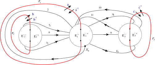
Figure 26.

Consider the standard diagram with $m_{2}>0,~{}m_{1}=m_{3}=0$ as in Figure 26. By referring to $(1)$ in Figure 24 we can have two possible diagrams to have $m_{2}>0$. We note that the other diagram can be obtained by reflecting the given diagram about the horizontal axis which is passing through the middles of $E_{i}^{\prime\prime}$. Then we have a similar argument to check the other case. So, it is enough to consider the diagram as in Figure 26.

We take a small open neighborhood $N^{\circ}(\epsilon)$ of $\epsilon$ so that $B^{3}-N^{\circ}(\epsilon)$ is a handlebody. Then $[\partial A]$ is the trivial element of $\pi_{1}(B^{3}-N^{\circ}(\epsilon))$ since $A$ is an essential disk in $B^{3}-\epsilon$.

Let $r_{i}$ be the simple arcs as in Figure 26. Then we note that the $r_{i}\cup\epsilon_{i}$ bound three disjoint disks in $B^{3}$. So, by considering the intersections between $\partial A$ and $r_{i}$ we can calculate the element $[\partial A]$ of $\pi_{1}(B^{3}-N^{\circ}(\epsilon),x_{0})$ as in Figure 26.

Now, we consider all the possible cases for the element $[\partial A]$ with respect to the three generators $a,b,c$ of $\pi_{1}(B^{3}-N^{\circ}(\epsilon),x_{0})$.

Consider the sequence of arc types in the standard diagram which carries $\partial A$. Then, we note that a subarc of $\partial A$ which is carried by one of the arcs in the standard diagram meets at most two times with $r_{1}\cup r_{2}\cup r_{3}$. The type $2$ and $11$ meet only $r_{1}$, the type $7$ meets only $r_{2}$ and the type $8$ meets only $r_{3}$, but the type $10$ meets $r_{1}$ and $r_{3}$ to have $(ac^{-1})^{\pm 1}$ with respect to the generators.

We note that the arc type $2$ carries $\partial A$ since $m_{2}>0$. So, we take the base point $x_{0}$ in $\partial E_{1}^{\prime\prime}$ as in Figure 26 and start with a subarc of $\partial A$ which is carried by the arc type $2$. Then we have $a^{\pm 1}$ with respect to the generators. Let $i_{1}$ be the upper arc type $i$ and $i_{2}$ be the lower arc type $i$ as in Figure 26. We note that if we show that $[\partial A]$ with the given orientation is not trivial then $[\partial A]$ with the other orientation is also not trivial.

Now, we give an orientation to each arc type $i$ as in Figure 26. We say an arc type $\overline{i}$ if the arc type $i$ has the opposite oriention of $i$.

We define a path $p$ of $\partial A$ so that $p\subset\partial A-E_{1}^{\prime\prime}$ and $|p\cap E_{1}^{\prime\prime}|=2$. We note that a path $p$ can break $E_{2}^{\prime\prime}$ or $E_{3}^{\prime\prime}$. A path $p$ is carried by some arc types. So, a path $p$ is represented by an arc type or a sequence of two types. For example, $2$ and $9~{}\overline{8_{1}}$ stand for paths. We also note that each path generates non-trivial element with respect to the generators.

Now, we consider all the cases for consecutive paths of length 2 to check whether or not there is a cancellation between two paths as follows, where the first element of each pair means consecutive paths of length 2 and the second element of each pair means the element for the given paths of length 2 with respect to the generators.

1. $(2|2,a^{-1}a^{-1})$, $(2|8_{i}~{}\overline{9},a^{-1}c)$, $(2|9~{}\overline{8_{i}},a^{-1}c^{-1})$, $(2|9~{}10,a^{-1}c^{-1}a^{-1})$ for $i=1,2$

2. $(\overline{2}|\overline{2},aa)$, $(\overline{2}|\overline{7_{i}}~{}6,ab^{-1})$, $(\overline{2}|\overline{6}~{}7_{i},ab)$ for $i=1,2$

3. $(\overline{6}~{}7_{i}|2,ba^{-1})$, $(\overline{6}~{}7_{i}|8_{j}~{}\overline{9},bc)$, $(\overline{6}~{}7_{i}|9~{}\overline{8_{j}},bc^{-1})$, $(\overline{6}~{}7_{i}|9~{}10,bc^{-1}a^{-1})$, $(\overline{6}~{}7_{i}|8_{2}~{}11,bca^{-1})$ for $i,j=1,2$

4. $(\overline{7_{i}}~{}6|2,b^{-1}a^{-1})$, $(\overline{7_{i}}~{}6|8_{j}~{}\overline{9},b^{-1}c)$, $(\overline{7_{i}}~{}6|9~{}\overline{8_{j}},b^{-1}c^{-1})$, $(\overline{7_{i}}~{}6|9~{}10,b^{-1}c^{-1}a^{-1})$, $(\overline{7_{i}}~{}6|8_{2}~{}11,b^{-1}ca^{-1})$ for $i,j=1,2$

5. $(8_{1}~{}\overline{9}|\overline{2},ca)$, $(8_{1}~{}\overline{9}|\overline{6}~{}7_{i},cb)$, $(8_{1}~{}\overline{9}|\overline{7_{i}}~{}6,cb^{-1})$, $(8_{1}~{}\overline{9}|\overline{10}~{}\overline{9},cac)$ for $i=1,2$

6. $(8_{2}~{}\overline{9}|\overline{2},ca)$, $(8_{2}~{}\overline{9}|\overline{6}~{}7_{i},cb)$, $(8_{2}~{}\overline{9}|\overline{7_{i}}~{}6,cb^{-1})$, $(8_{2}~{}\overline{9}|\overline{10}~{}\overline{9},cac)$, $(8_{2}~{}\overline{9}|\overline{10}~{}11,caca^{-1})$, $(8_{2}~{}\overline{9}|\overline{11}~{}10,cac^{-1}a^{-1})$, $(8_{2}~{}\overline{9}|\overline{11}~{}\overline{8_{2}},cac^{-1})$ for $i=1,2$

7. $(8_{2}~{}11|8_{2}~{}11,ca^{-1}ca^{-1})$, $(8_{2}~{}11|9~{}\overline{8_{2}},ca^{-1}a^{-1})$

8. $(9~{}\overline{8_{1}}|\overline{2},c^{-1}a)$, $(9~{}\overline{8_{1}}|\overline{6}~{}7_{i},c^{-1}b)$, $(9~{}\overline{8_{1}}|\overline{7_{i}}~{}6,c^{-1}b^{-1})$, $(9~{}\overline{8_{1}}|\overline{10}~{}\overline{9},c^{-1}ac)$ for $i=1,2$

9. $(9~{}\overline{8_{2}}|\overline{2},c^{-1}a)$, $(9~{}\overline{8_{2}}|\overline{6}~{}7_{i},c^{-1}b)$, $(9~{}\overline{8_{2}}|\overline{7_{i}}~{}6,c^{-1}b^{-1})$, $(9~{}\overline{8_{2}}|\overline{10}~{}\overline{9},c^{-1}ac)$, $(9~{}\overline{8_{2}}|\overline{10}~{}11,c^{-1}aca^{-1})$, $(9~{}\overline{8_{2}}|\overline{11}~{}10,c^{-1}ac^{-1}a^{-1})$, $(9~{}\overline{8_{2}}|\overline{11}~{}\overline{8_{2}},c^{-1}ac^{-1})$ for $i=1,2$

10. $(9~{}10|8_{i}~{}\overline{9},c^{-1}a^{-1}c)$, $(9~{}10|9~{}\overline{8_{i}},c^{-1}a^{-1}c^{-1})$, $(9~{}10|9~{}10,c^{-1}a^{-1}c^{-1}a^{-1})$ for $i=1,2$

11. $(\overline{10}~{}\overline{9}|\overline{2},aca)$, $(\overline{10}~{}\overline{9}|\overline{6}~{}7_{i},acb)$, $(\overline{10}~{}\overline{9}|\overline{7_{i}}~{}6,acb^{-1})$, $(\overline{10}~{}\overline{9}|\overline{10}~{}\overline{9},acac)$, $(\overline{10}~{}\overline{9}|\overline{10}~{}11,acaca^{-1})$, $(\overline{10}~{}\overline{9}|\overline{11}~{}10,acac^{-1}a^{-1})$ for $i=1,2$

12. $(\overline{10}~{}11|8_{2}~{}\overline{9},aca^{-1}c)$, $(\overline{10}~{}11|9~{}\overline{8_{2}},aca^{-1}c^{-1})$, $(\overline{10}~{}11|9~{}10,aca^{-1}c^{-1}a^{-1})$

13. $(\overline{11}~{}10|8_{2}~{}\overline{9},ac^{-1}a^{-1}c)$, $(\overline{11}~{}10|9~{}\overline{8_{2}},ac^{-1}a^{-1}c^{-1})$, $(\overline{11}~{}10|9~{}10,ac^{-1}a^{-1}c^{-1}a^{-1})$

We note that the path $2$ cannot be the next path of paths $9~{}10$, $\overline{11}~{}10$, $8_{2}~{}11$ and $\overline{10}~{}11$. Otherwise, $\partial A$ has an infinite spiral. Similarly, the paths $\overline{10}~{}\overline{9}$, $\overline{10}~{}11$, $\overline{11}~{}\overline{8_{2}}$ and $\overline{11}~{}10$ cannot be the next path of the path $\overline{2}$.

By considering all the cases, we note that there is no cancellation between two consecutive paths with respect to the generators $a,b,c$. This implies that $[\partial A]\neq e$ since $\pi_{1}(B^{3}-N^{\circ}(\epsilon),x_{0})$ is a free group. However, $[\partial A]=e$ since $A$ is an essential disk in $B^{3}-\epsilon$. This contradicts the assumption that $m_{1}=m_{3}=0$, $m_{2}>0$ and this completes the proof. ∎

Lemma 8.2.

Suppose that $\gamma^{\prime}$ is a simple closed curve which is parameterized by $(p_{1},q_{1},0,p_{2},q_{2},$ $0,p_{3},q_{3},0)$. If $x_{11}>0$, then we can construct a simple closed curve $\gamma_{0}$ which is parameterized by $(p_{1},q_{1},t_{1},p_{2},q_{2},t_{2},p_{3},q_{3},t_{3})$ for $t_{i}\in\mathbb{Z}$ as in the table below, and it bounds an essential disk in $B^{3}-\epsilon$ if $\gamma^{\prime}$ does. Moreover, each component of $\gamma_{0}\cap I^{\prime}$ is carried by one of the given arc types in one of the standard diagrams.

1. $q_{1}+p_{1}<x_{11}+x_{13}:$ $(t_{1},t_{2},t_{3})=(0,-1,0)$ if $p_{2}\neq 0$, $(t_{1},t_{2},t_{3})=(0,0,0)$ if $p_{2}=0$.
   

2. $q_{1}+p_{1}\geq x_{11}+x_{13}:$ $(t_{1},t_{2},t_{3})=(-1,-1,0)$ if $p_{2}\neq 0$, $(t_{1},t_{2},t_{3})=(-1,0,0)$ if $p_{2}=0$.

Moreover, if we have the following condition then $\gamma^{\prime}$ does not bound an essential disk in $B^{3}-\epsilon$.

1. $x_{11}+x_{13}\leq q_{1}+p_{1}<x_{11}+x_{12}+x_{13}$ and $x_{13}\geq q_{1}$.

Figure 27. The TWP diagram

Proof.

Consider a diagram which is called the train tracks-window-pattern diagram or the TWP diagram as in Figure 27. We note that $\gamma^{\prime}$ meets $\partial E_{i}^{\prime}$ only at the windows $\omega_{i}$ for $i=1,2,3$ in the TWP diagram. Let $a,b,\cdot\cdot\cdot,l$ be the weights for the train tracks as in Figure 27. We also consider $a,b,\cdot\cdot\cdot,l$ as the types of arcs. Then we can get the 11 types of essential arcs in $I^{\prime}$ as in the pattern diagram. (See Figure 23.) Then we can realize each connectivity pattern in the pattern diagram by an arc carried by this train track. For instance, the arcs for type 1 are carried by only $g-e-g$ and the arcs for type 3 are carried by $f-e-f$, $h-e-f$ or $h-e-h$.

We note that $|\gamma^{\prime}\cap\omega_{1}|=2p_{1}=2e+d+i$, $q_{1}=h$, $x_{11}=e$ and $x_{13}=i$.

We will now define the standard diagram by modifying the arcs carried by the train track so that they may lie outside the windows.

We set $t_{i}=0$ if $p_{i}=0$.

Figure 28.

In order to consider all the possible cases, we modify the diagram of Figure 27 into the diagram $(a)$ of Figure 28, Figure 29 and Figure 30 by the following three subcases.

Case 1: $q_{1}+p_{1}<x_{11}+x_{13}$. (See the diagram $(a)$ of Figure 28.) We note that $q_{1}+p_{1}=h+g<e+i=x_{11}+x_{13}$. Because of the given inequality $h+g<e+i$, we can have the black boxes $BB_{1}$ and $BB_{3}$ for the connectivities. Then we can consider the two more black boxes $BB_{2}$ and $BB_{4}$ for the rest of connectivities of subarcs. We say that the left incoming arc of $BB_{i}$ is input of $BB_{i}$ and the right incoming arc arc of $BB_{i}$ is output of $BB_{i}$. We note that $f_{2}>0$ since $h+g<e+i$. So, we have only one possible output of $BB_{1}$ which is called $f_{1}$. We note that $f_{1}+f_{2}=f$. Then the following are all possible connectivities of arcs having arc types from the diagram $(a)$ of Figure 28, where $i_{1}$ is the upper type $i$ and $i_{2}$ is the lower type $i$. Also, we define $m_{k_{i}}$ as the weight of the types $k_{1}$ and $k_{2}$ if $\gamma$ has two different isotopy types for type $k$. Clearly, we have $m_{k}=m_{k_{1}}+m_{k_{2}}$.

We claim that the diagram $(b)$ contains all the possible arc types which are obtained from the diagram $(a)$.

1. We start from $E_{1}^{\prime\prime-}$ with $f_{1}$. Then $f_{1}-e-(h+g)-h$ gives $x$, $f_{1}-e-(h+g)-g$ gives $2$, $f_{1}-e-f_{2}$ gives $3$, $f_{1}-c$ gives $6_{1}$, $f_{1}-b$ gives $7$ and $f_{1}-a$ gives $6_{2}$.
   

2. We start from $E_{1}^{\prime\prime-}$ with $f_{2}$. Then $f_{2}-i-j$ gives $y$, $f_{2}-i-k$ gives $11_{2}$ and $f_{2}-i-l$ gives $10_{2}$.
   

3. We start from $E_{1}^{\prime\prime-}$ with $g$. Then $g-(h+g)-i-j$ gives $8_{1}$, $g-(h+g)-i-k$ gives $9$ and $g-(h+g)-i-l$ gives $8_{2}$.
   

4. We start from $E_{1}^{\prime\prime-}$ with $h$. Then $h-(h+g)-i-j$ gives $10_{1}$, $h-(h+g)-i-k$ gives $11_{1}$ and $h-i-l$ gives $z$.
   

   We note that there is no subarc in $I^{\prime}$ which connects $E_{2}^{\prime\prime}$ and $E_{3}^{\prime\prime}$. Now, we exclude some cases as follows.
   

   Claim 1: $x$ cannot be realized.

   Proof.

   If $m_{x}>0$ then $m_{8}=m_{9}=m_{10_{2}}=m_{11_{2}}=0$. Then we note that $|\gamma^{\prime}\cap(\partial E_{1}^{\prime\prime}\cap E_{1}^{\prime\prime+})|=m_{2}$. However, $|\gamma^{\prime}\cap(\partial E_{1}^{\prime\prime}\cap E_{1}^{\prime\prime+})|\geq m_{2}+2m_{x}$. Because of the connnectivity in $E_{1}^{\prime\prime}$, we have an inequality $m_{2}\geq m_{2}+2m_{x}$. This violates the assumption that $m_{x}>0$. Therefore $m_{x}=0$.

   ∎

   Claim 2: $y$ and $z$ cannot be realized.

   Proof.

   If there is an arc for $y$ then the arc for type $8_{1}$ is the only possible arc which connects $E_{1}^{\prime\prime+}$ and $E_{3}^{\prime\prime+}$ and there is no arc to connect $E_{1}^{\prime\prime+}$ and $E_{3}^{\prime\prime-}$. We note that $m_{8_{1}}<j$ if there is an arc for $y$. We have the equality $j+l=k$ for the connectivity in $E_{3}^{\prime\prime}$. We point out that $m_{y}\neq 0$ implies $m_{2}=0$, so the only arc entering $E_{1}^{\prime\prime+}$ is $8_{1}$. Now, we have the inequality $m_{8_{1}}>l+k$ for the connectivity in $E_{1}^{\prime\prime}$. So, $m_{8_{1}}>l+k=l+(j+l)=j+2l$. This implies that $m_{8_{1}}>j$. This contradicts that $m_{8_{1}}<j$.
   

   If there is an arc for $z$ then we note that the two arcs $2$ and $8_{2}$ are the only arcs that can enter $E_{1}^{\prime\prime+}$. We note that $m_{8_{2}}<l$ if there is an arc for $z$. We still have the equality $j+l=k$. Then, we have the inequality that $m_{8_{2}}>k+j=(j+l)+j=2j+l$ for the connectivity in $E_{1}^{\prime\prime}$. So, $m_{8_{2}}>l$. This contradicts that $m_{8_{2}}<l$. ∎

Now, we set $t_{1}=0$ and $t_{2}=-1$ if $p_{2}\neq 0$ by applying a half Dehn twist supported on $E_{2}^{\prime\prime}$ clockwise to have $\gamma_{0}$ in the diagram $(c)$ of Figure 28. We set $t_{2}=0$ if $p_{2}=0$. Also, we set $t_{3}=0$. We note that the numbers on the diagram $(c)$ does not match with the numbers of the diagram $(b)$ in Figure 28 since the numbers came from the pattern diagram. Then, we can check that every component of $\gamma_{0}\cap I^{\prime}$ is isotopic to one of the arcs in the standard diagram 24 $(1)$.

We note that $\gamma^{\prime}$ bounds a disk in $B^{3}-\epsilon$ if and only if $\gamma_{0}$ bounds a disk in $B^{3}-\epsilon$ by Lemma 6.1.

Figure 29.

Case 2: $x_{11}+x_{13}\leq q_{1}+p_{1}<x_{11}+x_{12}+x_{13}$. (See the diagram $(a)$ of Figure 29.) First, in the diagram $(a)$ we note that $m_{1}=0$.

Because of the given inequalities $x_{11}+x_{13}\leq q_{1}+p_{1}<x_{11}+x_{12}+x_{13}$, we need to have the three black boxes $BB_{1},BB_{2}$ and $BB_{3}$, where $n_{1}\geq 0$ and $f-e>0$ since $x_{12}>0$. We note that the sum of the inputs of $BB_{1}$ and $BB_{2}$ is $x_{11}+x_{12}+x_{13}$. All the output of $BB_{2}$ should be the input of $BB_{3}$ since $x_{11}+x_{13}\leq q_{1}+p_{1}$.

Now, we get the diagram $(b)$ of Figure 29 by setting $t_{1}=t_{2}=-1$ if $p_{2}\neq 0$. If $p_{2}=0$ then set $t_{2}=0$. Set $t_{3}=0$.

We claim that the diagram $(c)$ of Figure 29 contains all the possible arc types which can be obtained from the diagram $(b)$.

The following are all possible connectivities of arcs having arc types from the diagram $(b)$ of Figure 29.

1. We start from $E_{1}^{\prime\prime+}$ with $e$. Then $e-n_{2}-g$ gives $2$ and $e-n_{2}-h$ gives $1$.
   

2. We start from $E_{1}^{\prime\prime+}$ with $f-e$. Then $(f-e)-c$ gives $5_{1}$, $(f-e)-b$ gives $4_{1}$ and $(f-e)-a$ gives $x$.
   

3. We start from $E_{1}^{\prime\prime-}$ with $g$. Then $g-n_{1}-c$ gives $7_{1}$, $g-n_{2}-b$ gives $6$ and $g-n_{1}-a$ gives $7_{2}$. We note that $g-n_{2}$ cannot take $i$ since $x_{13}<q_{1}$.
   

4. We start from $E_{1}^{\prime\prime+}$ with $h$. Then $h-n_{1}-c$ gives $y$, $h-n_{1}-b$ gives $4_{2}$, $h-n_{1}-a$ gives $5_{2}$, $h-n_{2}-i-j$ gives $8_{1}$, $h-n_{2}-i-k$ gives $9$ and $h-n_{2}-i-l$ gives $8_{2}$.

Claim: $x$ and $y$ cannot be realized.

Proof.

Assume that there is a subarc to realize $x$. Then, there is no arc to connect $E_{1}^{\prime\prime-}$ and $E_{2}^{\prime\prime+}$. So, $m_{4_{1}}>m_{5}+m_{7_{2}}$ for the connectivity in $E_{2}^{\prime\prime}$ since $m_{x}>0$. Also, we have an inequality $m_{7_{2}}+m_{2}\geq m_{2}+m_{4_{1}}+m_{5}$ for the connectivity in $E_{1}^{\prime\prime}$. By combining these two inequalities, we have $m_{4_{1}}>m_{5}+m_{7_{2}}\geq m_{5}+(m_{4_{1}}+m_{5})=m_{4_{1}}+2m_{5}$. However, this is impossible to satisfy. Therefore, the assumption fails.

Now, assume that there is a subarc to realize $y$. Then, there is no arc to connect $E_{1}^{\prime\prime-}$ and $E_{2}^{\prime\prime+}$. So, $m_{4_{2}}>m_{5}+m_{7_{1}}$ for the connectivity in $E_{2}^{\prime\prime}$ since $m_{y}>0$. Also, we note that the arc $7_{1}$ is the only arc that can enter $E_{1}^{\prime\prime-}$. This makes an inequality $m_{7_{1}}>m_{4_{2}}+m_{5}$ for the connectivity in $E_{1}^{\prime\prime}$. By combining these two inequalities, we have $m_{4_{2}}>m_{5}+m_{7_{1}}\geq m_{5}+(m_{4_{2}}+m_{5})=m_{4_{2}}+2m_{5}$. However, this is impossible to satisfy. Therefore, the assumption fails.

∎

We note that if $x_{13}\geq q_{1}$, then $m_{1}=0$ because in the diagram $(b)$ every subarc of $\gamma^{\prime}$ carried by $e$ starts from $E_{1}^{\prime\prime+}$ and ends at $E_{1}^{\prime\prime-}$ in the diagram $(b)$ in Figure 29. Also, $m_{3}=0$ in the diagram $(b)$ since $m_{1}=0$ in the diagram $(a)$. Therefore, $m_{1}+m_{3}=0$. In this case, $\gamma^{\prime}$ cannot bound an essential disk in $B^{3}-\epsilon$ by Lemma 8.1.

Thus, we can check that every component of $\gamma_{0}\cap I^{\prime}$ is isotopic to one of the arcs in the standard diagram 24 $(2)$.

Figure 30.

Case 3: $x_{11}+x_{12}+x_{13}\leq q_{1}+p_{1}$. (See the diagram $(a)$ of Figure 30.) We have the black box $BB_{2}$ for the given inequality. We note the sum of the inputs of $BB_{2}$ is $x_{11}+x_{12}+x_{13}$ and the sum of the outputs of $BB_{3}$ is $q_{1}+p_{1}$. We note that $n_{2}=x_{11}+x_{12}+x_{13}$.

Then, we set $t_{1}=-1$, and we set $t_{2}=-1$ if $p_{2}>0$ and $t_{2}=0$ if $p_{2}=0$. Also we set $t_{3}=0$ to have the diagram $(b)$ of Figure 30.

Then we have two subcases as follows. We refer to the diagram $(b)$.

Subcase 1: If $x_{13}\geq q_{1}$ then we note that $m_{1}=0$ since every arc which starts from $E_{1}^{\prime\prime+}$ with $f$ should end at $E_{1}^{\prime\prime-}$.

Now, we claim that the diagram $(c)$ of Figure 30 contains all the possible arc types which are obtained from the diagram $(b)$.

The following are the connectivities of arcs having arc types from the diagram $(b)$ of Figure 30.

1. We start from $E_{1}^{\prime\prime+}$ with $f$. Then $f-e-n_{2}-g$ gives $2$. We note that $m_{1}=0$ implies $f-e-n_{2}-h$ does not occur.

2. We start from $E_{1}^{\prime\prime-}$ with $g$. Then $g-n_{1}-e-n_{2}-g$ gives $3$, $g-n_{2}-c$ gives $7_{1}$, $g-n_{2}-b$ gives $6$, $g-n_{2}-a$ gives $7_{2}$, $g-n_{2}-i-j$ gives $w$, $g-n_{2}-i-k$ gives $11$ and $g-n_{2}-i-l$ gives $10$. We note that $g-n_{1}-e-n_{2}-h$ does not exist since every arc starting from $E_{1}^{\prime\prime-}$ with $g-n_{1}-e-n_{2}$ should connect to $g$ since $x_{13}=i\geq h=q_{1}$.
   

3. We start from $E_{1}^{\prime\prime+}$ with $h$. Then $h-n_{2}-i-j$ gives $8_{1}$, $h-n_{2}-i-k$ gives $9$ and $h-n_{2}-i-l$ gives $8_{2}$.
   

   Claim: $w$ cannot be realized.

   Proof.

   Suppose that there is a subarc to realize $m_{w}>0$. Then, we note that the arcs $2$ and $8_{1}$ are the only two arcs that can enter $E_{1}^{\prime\prime+}$. This makes an inequality $m_{8_{1}}+m_{2}>m_{2}+m_{10}+m_{11}+m_{w}$ for the connectivity in $E_{1}^{\prime\prime}$ since $m_{3}>0$ by Lemma 8.1. This implies that $m_{8_{1}}>m_{10}+m_{11}+m_{w}$. We also have an equality $m_{w}+m_{8_{1}}+m_{10}=m_{11}$ for the connectivity in $E_{3}^{\prime\prime}$. By combining this inequality and equality, we have $m_{11}=m_{w}+m_{8_{1}}+m_{10}>m_{w}+m_{10}+m_{11}+m_{w}+m_{10}>m_{11}$ since $m_{w}>0$. However, this is impossible to satisfy. Therefore, the assumption fails. ∎

   Thus, we can check that every component of $\gamma_{0}\cap I^{\prime}$ is isotopic to one of the arcs in the standard diagram 24 $(1)$.
   

Figure 31.

Subcase 2: If $x_{13}<q_{1}$ then $m_{1}>0$ since $e>0$ because $x_{11}>0$.

The following are the connectivities of arcs having arc types from the diagram $(b)$ of Figure 30. We claim that the diagram $(b)$ of Figure 31 contains all the possible arc types.

1. We start from $E_{1}^{\prime\prime+}$ with $f$. Then $f-e-n_{2}-h$ gives $1$ and $f-e-n_{2}-g$ gives $2_{2}$.
   

2. We start from $E_{1}^{\prime\prime-}$ with $g$. Then $g-n_{1}-e-n_{2}-h$ gives $2_{1}$, $g-n_{1}-e-n_{2}-g$ gives $3$, $g-n_{2}-c$ gives $7_{1}$, $g-n_{2}-b$ gives $6$ and $g-n_{2}-a$ gives $7_{2}$.
   

   We note that $g-n_{2}-i-j$, $g-n_{2}-i-k$ and $g-n_{2}-i-l$ do not exist since no arc starting from $E_{1}^{\prime\prime-}$ with $g-n_{2}$ can go to $i$ since $i<h$.
   

3. We start from $E_{1}^{\prime\prime+}$ with $h$. Then $h-n_{1}-e-n_{2}-h$ gives $x$, $h-n_{2}-c$ gives $y$, $h-n_{2}-b$ gives $4_{2}$, $h-n_{2}-a$ gives $5_{2}$, $h-n_{2}-i-j$ gives $8_{1}$, $h-n_{2}-i-k$ gives $9$ and $h-n_{2}-i-l$ gives $8_{2}$.
   

   Claim: $x$ and $y$ cannot be realized.

   Proof.

   First, assume that there is a subarc to realize $m_{x}>0$. Then we note that $2_{1}$ is the only possible arc which can enter to the $E_{1}^{\prime\prime-}$. Because of the connectivity in $E_{1}^{\prime\prime}$, we have an inequality $m_{2_{1}}\geq m_{2_{1}}+m_{x}$. This implies that $m_{2_{1}}>m_{2_{1}}$ since $x>0$. However, this is impossible to satisfy. Therefore, $m_{x}=0$.
   

   Now, assume that there is a subarc to realize $m_{y}>0$. Then we note that $4_{2}$ is the only possible arc which can enter to the $E_{2}^{\prime\prime+}$. We have an equality $m_{4_{2}}=m_{y}+m_{7_{1}}+m_{5_{2}}$ for the connectivity in $E_{2}^{\prime\prime}$. Also, we have an inequality $m_{7_{1}}\geq m_{y}+m_{4_{2}}+m_{5_{2}}$ for the connectivity in $E_{1}^{\prime\prime}$. Therefore, we have $m_{7_{1}}\geq m_{y}+m_{4_{2}}+m_{5_{2}}=m_{y}+(m_{y}+m_{7_{1}}+m_{5_{2}})+m_{5_{2}}>m_{7_{1}}$ since $m_{y}>0$. This is impossible to satisfy. Therefore, $m_{y}=0$.

   ∎

Thus, we can check that every component of $\gamma_{0}\cap I^{\prime}$ is isotopic to one of the arcs in the standard diagram 24 $(2)$.

By combining cases 1, 2 and 3, we note that $\gamma^{\prime}$ can be modified as a simple closed curve $\gamma_{0}$ so that all components of $\gamma_{0}\cap I^{\prime}$ are isotopic to arcs of the two diagrams in Figure 24, but $\gamma_{0}$ bounds an essential disk if $\gamma^{\prime}$ does by Lemma 6.1.

∎

We represent $\gamma_{0}$ by putting weights on these arcs.

Now, we want to calculate $m_{i}$ of $\gamma_{0}$ for $i=1,2,...,11$ by using the parameters $p_{j},q_{j}$ of $\gamma^{\prime}$ for $j=1,2,3$.

The following is the table of $m_{i}$ for each case.

Lemma 8.3.

1. $x_{11}+x_{13}>q_{1}+p_{1}$:
   

   $m_{3}=p_{3}-p_{2}-q_{1}$, $m_{2}=q_{1}+p_{1}-2p_{3}$, $m_{7_{1}}=q_{2}$, $m_{7_{2}}=p_{2}-q_{2}$, $m_{6}=p_{2}$, $m_{10_{1}}=\min(q_{1},p_{3}-q_{3})$, $m_{10_{2}}=\min(0,\max(2p_{3}-p_{1}-q_{1},0),q_{3})$, $m_{11_{1}}=\max(0,q_{1}-p_{3}+q_{3})$, $m_{11_{2}}=\max(0,\max(2p_{3}-p_{1}-q_{1},0)-q_{3})$, $m_{8_{1}}=\max(0,p_{3}-q_{3}-p_{1})$, $m_{8_{2}}=\max(0,q_{3}-\max(2p_{3}-p_{1}-q_{1},0))$, $m_{9}=m_{10}+m_{8}-m_{11}.$
   

2. $x_{11}+x_{13}\leq q_{1}+p_{1}$ and $x_{13}<q_{1}$:
   

   $(a)$ $q_{1}>x_{13}+x_{11}$: $m_{1}=p_{1}-p_{2}-p_{3}$, $m_{8_{1}}=p_{3}-q_{3},~{}m_{8_{2}}=q_{3},~{}m_{9}=p_{3}$, $m_{5_{1}}=\min(q_{2},p_{2}+p_{3}-q_{1})$, $m_{7_{1}}=q_{2}-m_{5_{1}},~{}m_{4_{1}}=p_{2}+p_{3}-q_{1}-m_{5_{1}}$, $m_{5_{2}}=\min(p_{2}-q_{2},q_{1}+p_{2}-p_{1}-p_{3}),~{}m_{7_{2}}=p_{2}-q_{2}-m_{5_{2}},~{}m_{4_{2}}=q_{1}+p_{2}-p_{1}-p_{3}-m_{5_{2}}$, $m_{6}=m_{5}+m_{7}-m_{4}$.
   

   $(b)$ $x_{13}<q_{1}\leq x_{13}+x_{11}$: $m_{1}=q_{1}-2p_{3},~{}m_{8_{1}}=p_{3}-q_{3},~{}m_{8_{2}}=q_{3},~{}m_{9}=p_{3}$, $m_{2}=p_{1}+p_{3}-p_{2}-q_{1}$, $m_{5_{1}}=\min(q_{2},p_{2}+p_{3}-q_{1}),~{}m_{7_{1}}=q_{2}-m_{5_{1}},~{}m_{4_{1}}=p_{2}+p_{3}-q_{1}-m_{5_{1}},m_{7_{2}}=p_{2}-q_{2}$, $m_{6}=m_{5}+m_{7}-m_{4}$.
   

3. $x_{11}+x_{12}+x_{13}\leq q_{1}+p_{1}$:
   

   1. $x_{13}\geq q_{1}$:
      

      $m_{3}=q_{1}-p_{2}-p_{3}$, $m_{2}=p_{1}-q_{1}$, $m_{7_{1}}=q_{2}$, $m_{7_{2}}=p_{2}-q_{2},$ $m_{6}=p_{2}$, $m_{8_{1}}=\min(q_{1},p_{3}-q_{3})$, $m_{8_{2}}=\max(q_{3}-(2p_{3}-q_{1}),0),$ $m_{10}=\min(2p_{3}-q_{1},q_{3})$, $m_{11}=\max((2p_{3}-q_{1})-q_{3},0)$.
      

   2. $x_{13}<q_{1}$, $p_{1}\geq 2q_{1}-2p_{3}$: $m_{2_{2}}=p_{1}+2p_{3}-2q_{1}$, $m_{1}=q_{1}-2p_{3}$, $m_{3}=q_{1}-p_{2}-p_{3}$, $m_{7_{1}}=q_{2}$, $m_{7_{2}}=p_{2}-q_{2}$, $m_{6}=p_{2}$, $m_{8_{1}}=p_{3}-q_{3}$, $m_{8_{2}}=q_{3}$ and $m_{9}=p_{3}$.
      

   3. $x_{13}<q_{1}$, $p_{1}<2q_{1}-x_{13}$:
      

      1. $q_{1}>x_{13}+x_{11}$: $m_{2_{1}}=q_{1}-p_{2}-p_{3}$, $m_{1}=p_{1}-q_{1}$, $m_{7_{1}}=q_{2}$, $m_{5_{2}}=\min(p_{2}-q_{2},q_{1}-x_{11}-x_{13})$, $m_{7_{2}}=p_{2}-q_{2}-m_{5_{2}}=p_{2}-q_{2}-\min(p_{2}-q_{2},q_{1}+p_{2}-p_{1}-p_{3})$, $m_{4_{2}}=q_{1}+p_{2}-p_{1}-p_{3}-m_{5_{2}}=q_{1}+p_{2}-p_{1}-p_{3}-\min(p_{2}-q_{2},q_{1}+p_{2}-p_{1}-p_{3})$, $m_{6}=p_{2}-m_{4_{2}}=p_{1}+p_{3}-q_{1}+\min(p_{2}-q_{2},q_{1}+p_{2}-p_{1}-p_{3})$, $m_{8_{1}}=p_{3}-q_{3}$, $m_{8_{2}}=q_{3}$ and $m_{9}=p_{3}$.
         

      2. $q_{1}\leq x_{13}+x_{11}$: $m_{2_{1}}=2q_{1}-p_{1}-2p_{3}$, $m_{1}=p_{1}-q_{1}$, $m_{3}=p_{1}+p_{3}-p_{2}-q_{1}$, $m_{7_{1}}=q_{2}$, $m_{7_{2}}=p_{2}-q_{2}$, $m_{6}=p_{2}$, $m_{8_{1}}=p_{3}-q_{3}$, $m_{8_{2}}=q_{3}$ and $m_{9}=p_{3}$.

Figure 32.

Proof.

Consider $\gamma_{0}$ which is in standard position.

First, we recall that $x_{ij}=I_{j},~{}x_{ik}=I_{k}$ and $x_{ii}={I_{i}-I_{j}-I_{k}\over 2}$ if $x_{11}>0$ by the equations in Lemma 5.1. Also, we note that $I_{1}=2p_{1},I_{2}=2p_{2}$ and $I_{3}=2p_{3}$. So, we can have $x_{11}=p_{1}-p_{2}-p_{3}$, $x_{12}=2p_{2}$ and $x_{13}=2p_{3}$ from the equations.

Case 1: $x_{11}+x_{13}>q_{1}+p_{1}$. Refer to the diagrams of Figure 28 and Figure 32 to get the weights $m_{i}$ as follows.

First, we note the weight of the bottom arc starting from $E_{1}^{\prime\prime-}$ is $\max(x_{13}-(p_{1}+q_{1}),0)$ as in Figure 32 since if $m_{2}>0$ then the weight is zero and $x_{13}-(p_{1}+q_{2})<0$, and if $m_{2}=0$ then the weight is $x_{13}-(p_{1}+q_{1})$ because the weight starting from $E_{1}^{\prime\prime+}$ is $p_{1}$ in this case.

Then we have $m_{3}=f_{2}=(e+i)-(h+g)=(x_{11}+x_{13})-(q_{1}+p_{1})$, $m_{2}=x_{11}-m_{3}=(q_{1}+p_{1})-x_{13}$, $m_{7_{1}}=q_{2}$, $m_{7_{2}}=p_{2}-q_{2},$ $m_{6}=p_{2}$.

We note that $m_{10_{1}}=\min(q_{1},p_{3}-q_{3})$, $m_{10_{2}}=\min(\max(x_{13}-(p_{1}+q_{1}),0),q_{3})$. Then we have $m_{11_{1}}=\max(0,q_{1}-(p_{3}-q_{3}))$ since if $q_{1}\geq p_{3}-q_{3}$ then $m_{11_{1}}=q_{1}-(p_{3}-q_{3})$ and if $q_{1}<p_{3}-q_{3}$ then $m_{11_{1}}=0$. Similarly, we have $m_{11_{2}}=\max(0,\max(x_{13}-(p_{1}+q_{1}),0)-q_{3})$. Also, we have $m_{8_{1}}=\max(0,(p_{3}-q_{3})-q_{1})$ since if $p_{3}-q_{3}\geq q_{1}$ then $m_{8_{1}}=(p_{3}-q_{3})-q_{1}$ and if $p_{3}-q_{3}<q_{1}$ then $m_{18_{1}}=0$. Similarly, $m_{8_{2}}=\max(0,q_{3}-\max(x_{13}-(p_{1}+q_{1}),0))$. We note that $m_{9}=m_{10}+m_{8}-m_{11}.$

In order to have better formulas as in Lemma 8.3, use $x_{11}=p_{1}-p_{2}-p_{3}$, $x_{12}=2p_{2}$ and $x_{13}=2p_{3}$.

Case 2: $x_{11}+x_{13}\leq q_{1}+p_{1}<x_{11}+x_{12}+x_{13}$ and $x_{13}<q_{1}$.

Then we need to consider the following two cases in Figure 33 which are obtained from the diagram $(b)$ of Figure 29. We note that the first case has $m_{2}=0$ and the second case has $m_{2}>0$. By referring to the two diagrams of Figure 33, we can get the weights $m_{i}$ as follows. We will use a similar argument as in the first case to find $m_{5_{1}}$ and $m_{5_{2}}$.

Figure 33.

$(a)$ $q_{1}>x_{13}+x_{11}$: $m_{1}=x_{11}$, $m_{8_{1}}=p_{3}-q_{3},m_{8_{2}}=q_{3},m_{9}=p_{3}$, $m_{5_{1}}=\min(q_{2},x_{11}+x_{12}+x_{13}-(q_{1}+p_{1}))$, $m_{7_{1}}=q_{2}-m_{5_{1}},m_{4_{1}}=x_{11}+x_{12}+x_{13}-(q_{1}+p_{1})-m_{5_{1}}$, $m_{5_{2}}=\min(p_{2}-q_{2},q_{1}-(x_{11}+x_{13})),m_{7_{2}}=p_{2}-q_{2}-m_{5_{2}},m_{4_{2}}=q_{1}-(x_{11}+x_{13})-m_{5_{2}}$, $m_{6}=m_{5}+m_{7}-m_{4}$.

$(b)$ $x_{13}<q_{1}\leq x_{13}+x_{11}$: $m_{1}=q_{1}-x_{13},m_{8_{1}}=p_{3}-q_{3},m_{8_{2}}=q_{3},m_{9}=p_{3}$, $m_{2}=x_{11}+x_{13}-q_{1}$; $m_{5_{1}}=\min(q_{2},x_{11}+x_{12}+x_{13}-(q_{1}+p_{1})),m_{7_{1}}=q_{2}-m_{5_{1}},m_{4_{1}}=x_{11}+x_{12}+x_{13}-(q_{1}+p_{1})-m_{5_{1}},m_{7_{2}}=p_{2}-q_{2},$ $m_{6}=m_{5}+m_{7}-m_{4}$.

In order to have better formulas as in Lemma 8.3, use $x_{11}=p_{1}-p_{2}-p_{3}$, $x_{12}=2p_{2}$ and $x_{13}=2p_{3}$.

We recall that if $q_{1}\leq x_{13}$ then $\gamma^{\prime}$ does not bound an essential disk in $B^{3}-\epsilon$.

Case 3: $x_{11}+x_{12}+x_{13}\leq q_{1}+p_{1}$. We note that $q_{1}+p_{1}<2p_{1}$ since $0\leq q_{1}<p_{1}$. Then we have two cases for this.

Figure 34.

1. $x_{13}\geq q_{1}$: Refer to the diagram $(c)$ of Figure 30 and the diagram of Figure 34.
   

   Then we have the following formulas for $m_{j}$. We will use a similar argument as in the first case to find $m_{8_{1}},m_{8_{2}},m_{10}$ and $m_{11}$.
   

   $m_{3}=(q_{1}+p_{1})-(x_{11}+x_{12}+x_{13})$, $m_{2}=x_{11}-m_{3}=(2x_{11}+x_{12}+x_{13})-(q_{1}+p_{1})$, $m_{7_{1}}=q_{2}$, $w_{7_{2}}=p_{2}-q_{2},$ $w_{6}=p_{2}$, $m_{8_{1}}=\min(q_{1},p_{3}-q_{3})$, $m_{8_{2}}=\max(q_{3}-(2p_{3}-q_{1}),0)$, $m_{10}=\min(2p_{3}-q_{1},q_{3})$, $m_{11}=\max((2p_{3}-q_{1})-q_{3},0)$.
   

   

   Figure 35.

2. $x_{13}<q_{1}$:
   

   We have the diagram $(a)$ of Figure 35 by referring Figure 30 and Figure 31.
   

   Then we consider the two subcases $p_{1}-q_{1}\geq q_{1}-x_{13}$ and $p_{1}-q_{1}<q_{1}-x_{13}$.
   

3. : If $p_{1}-q_{1}\geq q_{1}-x_{13}$ then we can directly get the formulas for $m_{j}$ as follows. (Refer to the diagram $(b)$ of Figure 35.)
   

   $m_{2_{2}}=p_{1}+x_{13}-2q_{1}$, $m_{1}=q_{1}-x_{13}$, $m_{3}=x_{11}+q_{1}-p_{1}$, $m_{7_{1}}=q_{2}$, $m_{7_{2}}=p_{2}-q_{2}$, $m_{6}=p_{2}$, $m_{8_{1}}=p_{3}-q_{3}$, $m_{8_{2}}=q_{3}$ and $m_{9}=p_{3}$.
   

4. : If $p_{1}-q_{1}<q_{1}-x_{13}$ then we have the diagram $(c)$ of Figure 35.
   

   Now, we consider the two subcases for this which are $(i)~{}q_{1}>x_{13}+x_{11}$ or $(ii)~{}q_{1}\leq x_{13}+x_{11}$.
   

   

   Figure 36.

   Then we have the two diagrams of Figure 36
   

   1. $q_{1}>x_{13}+x_{11}$: (Refer to the diagram $(i)$ of Figure 36.)
      

      Then we get the formulas for $m_{j}$ as follows.
      

      $m_{2_{1}}=x_{11}+q_{1}-p_{1}$, $m_{1}=p_{1}-q_{1}$, $m_{7_{1}}=q_{2}$, $m_{5_{2}}=\min(p_{2}-q_{2},q_{1}-x_{11}-x_{13})$, $m_{7_{2}}=p_{2}-q_{2}-m_{5_{2}}=p_{2}-q_{2}-\min(p_{2}-q_{2},q_{1}-x_{11}-x_{13})$, $m_{4_{2}}=q_{1}-x_{11}-x_{13}-m_{5_{2}}=q_{1}-x_{11}-x_{13}-\min(p_{2}-q_{2},q_{1}-x_{11}-x_{13})$, $m_{6}=p_{2}-m_{4_{2}}=p_{2}-(q_{1}-x_{11}-x_{13}-\min(p_{2}-q_{2},q_{1}-x_{11}-x_{13}))=p_{2}-q_{1}+x_{11}+x_{13}+\min(p_{2}-q_{2},q_{1}-x_{11}-x_{13})$, $m_{8_{1}}=p_{3}-q_{3}$, $m_{8_{2}}=q_{3}$ and $m_{9}=p_{3}$.
      

   2. $q_{1}\leq x_{13}+x_{11}$: (Refer to the diagram $(ii)$ of Figure 36.)
      

      Then we get the formulas for $m_{j}$ as follows.
      

      $m_{2_{1}}=2q_{1}-p_{1}-x_{13}$, $m_{1}=p_{1}-q_{1}$, $m_{3}=x_{11}+x_{13}-q_{1}$, $m_{7_{1}}=q_{2}$, $m_{7_{2}}=p_{2}-q_{2}$, $m_{6}=p_{2}$, $m_{8_{1}}=p_{3}-q_{3}$, $m_{8_{2}}=q_{3}$ and $m_{9}=p_{3}$.
      

      In order to have better formulas as in Lemma 8.3, use $x_{11}=p_{1}-p_{2}-p_{3}$, $x_{12}=2p_{2}$ and $x_{13}=2p_{3}$.

∎

9. Step 4: Main Theorem

Now, we want to discuss the main theorem that can complete my algorithm. In order to do this, we define four homeomorphisms $(\delta_{1}\delta_{2}^{-1})^{\pm 1}$ and $\delta_{3}^{\pm 1}$ as follows.

Let $\delta_{1}$ and $\delta_{2}$ be the clockwise half Dehn twists supported on two punctured disks $C_{1}$ and $C_{2}$ respectively as in Figure 37. Also, let $\delta_{3}$ be clockwise half Dehn twists supported on two punctured disk $E_{4}^{\prime}$ as in Figure 38. Then we have the two following lemmas.

Lemma 9.1.

$\gamma_{0}$ bounds an essential disk in $B^{3}-\epsilon$ if and only if $(\delta_{1}\delta_{2}^{-1})^{\pm 1}(\gamma_{0})$ bounds an essential disk in $B^{3}-\epsilon$.

Figure 37. The homeomorphisms $\delta_{1}\delta_{2}^{-1}$ and $\delta_{2}\delta_{1}^{-1}$

Proof.

We notice that an extension $K$ to $B^{3}$ of $(\delta_{1}\delta_{2}^{-1})^{\pm 1}$ changes the position of two strings. So, it preseves the $\infty$ tangle. Let $A$ be the essential disk in $B^{3}-\epsilon$ so that $\partial A=\gamma_{0}$. Then, we know that $K(A)$ bounds a disk in $B^{3}-\epsilon$ and $K(\gamma_{0})$ is essential in $\Sigma_{0.6}$. Therefore, $(\delta_{1}\delta_{2}^{-1})^{\pm 1}(\gamma_{0})$ bounds an essential disk in $B^{3}-\epsilon$.

∎

Lemma 9.2.

$\gamma_{0}$ bounds an essential disk in $B^{3}-\epsilon$ if and only if $\delta_{3}(\gamma_{0})$ bounds an essential disk in $B^{3}-\epsilon$.

Proof.

By lemma 6.1, it is trivial. ∎

Figure 38. The homeomorphism $\delta_{3}$

Now, let $(p_{11},q_{11},t_{11},p_{21},q_{21},t_{21},p_{31},q_{31},t_{31})$ be the parameters for $h(\gamma_{0})$ for $h\in\{(\delta_{1}\delta_{2}^{-1})^{\pm 1},\delta_{3}^{\pm 1}\}$. Also, let $(p_{11},q^{\prime}_{11},p_{21},q^{\prime}_{21},p_{31},q^{\prime}_{31})$ be the Dehn’s parameters for $h(\gamma_{0})$, where $q^{\prime}_{i1}=p_{i1}t_{i1}+q_{i1}$ for $i=1,2,3$. We note that the nine parameters can be obtained from the Dehn’s parameters. Also, we know that $|\gamma_{0}\cap\partial E|=2(p_{1}+p_{2}+p_{3})$ and $|\delta_{1}^{-1}\delta_{2}(\gamma_{0})\cap\partial E|=2(p_{11}+p_{21}+p_{31})$.

Now, here is the main theorem.

Theorem 9.3.

Suppose that $\gamma_{0}$ bounds an essential disk in $B^{3}-\epsilon$ and $\gamma_{0}$ is in standard position in $I^{\prime}$ and $m_{3}>0$. Then applying one of the homeomorphisms $(\delta_{1}\delta_{2}^{-1})^{\pm 1}$ and $\delta_{3}^{\pm 1}$ reduces the sum of the $p_{i}$ for the image of $\gamma_{0}$. Especially, the following are the formulas for the Dehn’s parameter changes for each case.

1. $m_{2_{1}},m_{3}>0,m_{1}=0$ and $m_{3}>m_{2}+1$: $(p_{11},q^{\prime}_{11},p_{21},q^{\prime}_{21},p_{31},q^{\prime}_{31})=(p_{1}-2m_{2},q^{\prime}_{1}+m_{2}-(m_{10}+m_{11}),p_{2},q_{2}^{\prime},p_{3},q_{3}^{\prime}+2(m_{10}+m_{11}))$ by $\delta_{3}$.
   

2. $m_{2_{2}},m_{3}>0,m_{1}=0$ and $m_{3}>m_{2}+1$: $(p_{11},q^{\prime}_{11},p_{21},q^{\prime}_{21},p_{31},q^{\prime}_{31})=(p_{1}-2m_{2},q^{\prime}_{1}-m_{2}+(m_{10}+m_{11}),p_{2},q_{2}^{\prime},p_{3},q_{3}^{\prime}-2(m_{10}+m_{11}))$ by $\delta_{3}^{-1}$.
   

3. $m_{3}>m_{2}>0$: $(p_{11},q^{\prime}_{11},p_{21},q^{\prime}_{21},p_{31},q^{\prime}_{31})=(p_{1}-2m_{2},q^{\prime}_{1}+m_{2},p_{2},q_{2}^{\prime},p_{3},q^{\prime}_{3})$ by $\delta_{3}$.
   

4. $m_{1}>m_{2}\geq m_{3}>0$: $(p_{11},q^{\prime}_{11},p_{21},q^{\prime}_{21},p_{31},q^{\prime}_{31})=(p_{1}-2m_{2},q^{\prime}_{1}+(m_{3}-m_{2}),p_{2},q_{2}^{\prime},p_{3},q^{\prime}_{3})$ by $\delta_{3}$.
   

5. $m_{1}=m_{3}=1$ and $m_{i}=0$ for all $i\neq 1,3$: It bounds an essential disk in $B^{3}-\epsilon$.
   

6. $m_{1}=m_{2}=0$, $m_{3}\geq 2$.

   1. $m_{11}=0$: $(p_{11},q^{\prime}_{11},p_{21},q^{\prime}_{21},p_{31},q^{\prime}_{31})=(p_{1}-m_{8},q^{\prime}_{1}-m_{8_{1}},p_{2},q^{\prime}_{2},p_{3}-m_{8},q^{\prime}_{3}+m_{8})$ by $\delta_{1}^{-1}\delta_{2}$.
      

   2. $m_{8}=0$: $(p_{11},q^{\prime}_{11},p_{21},q^{\prime}_{21},p_{31},q^{\prime}_{31})=(p_{1}-m_{11},q^{\prime}_{1}-m_{11_{1}},p_{2},q^{\prime}_{2},p_{3}-m_{11},q^{\prime}_{3}+m_{11})$ by $\delta_{1}\delta_{2}^{-1}$.
      

   3. $m_{8},m_{11}>0$:
      

      1. $m_{8_{1}},m_{11_{2}}>0$: $(p_{11},q^{\prime}_{11},p_{21},q^{\prime}_{21},p_{31},q^{\prime}_{31})=(p_{1}-(m_{8_{1}}-m_{11_{2}}),q^{\prime}_{1}-m_{8_{1}},p_{2},q^{\prime}_{2},p_{3}-(m_{8_{1}}-m_{11_{2}}),q^{\prime}_{3}+m_{11_{2}})$ by $\delta_{1}^{-1}\delta_{2}$.
         

      2. $m_{8_{2}},m_{11_{1}}>0$: $(p_{11},q^{\prime}_{11},p_{21},q^{\prime}_{21},p_{31},q^{\prime}_{31})=(p_{1}-(m_{8_{2}}-m_{11_{1}}),q^{\prime}_{1}+m_{11_{1}},p_{2},q^{\prime}_{2},p_{3}-(m_{8_{2}}-m_{11_{1}}),q^{\prime}_{3}-m_{8_{2}})$ by $\delta_{1}^{-1}\delta_{2}$.

   Also, if $\gamma_{0}$ satisfies any of the following conditions then $\gamma_{0}$ does not bound an essential disk in $B^{3}-\epsilon$.
   

7. $m_{1}+m_{3}<2$ and $m_{i}>0$ for some $i$.
   

8. $m_{2},m_{3}>0,m_{1}=0$ and $m_{3}\leq m_{2}+1$.
   

9. $m_{2}\geq m_{1},m_{3}>0$.

Proof.

Suppose that $\gamma_{0}$ is parameterized by $(p_{1},q_{1},t_{1},p_{2},q_{2},t_{2},$ $p_{3},q_{3},0)$ to have $\gamma_{0}$ which is in standard position in $I^{\prime}$. We note that $t_{2}=0$ if $p_{2}=0$ and $t_{2}=-1$ if $p_{2}\neq 0$.

Figure 39.

First, we assume that $m_{2},m_{3}>0$ and $m_{1}=0$. We note that there are two type 2 in a standard diagram and they cannot coexist. Without loss of generality, we choose the diagram $(a)$ as in Figure 39.

Then we apply $\delta_{3}$ to $\partial A$ to reduce the minimal intersection number of $\gamma_{0}$ with $\partial E$. The diagram $(b)$ of Figure 39 shows there is no possibility to have $x_{22}>0$ or $x_{33}>0$ for $\delta_{3}(\gamma_{0})$.

We note that if $m_{3}\leq m_{2}+1$ then $x_{11}$ of $\delta_{3}(\gamma_{0})$ is less than $2$. Therefore, $\delta_{3}(\gamma_{0})$ does not bound an essential disk in $B^{3}-\epsilon$ since $x_{11}\geq 2$ if $\delta_{3}(\gamma_{0})$ bounds an essential disk in $B^{3}-\epsilon$. This implies that $\gamma_{0}$ also does not bound an essential disk in $B^{3}-\epsilon$. This makes a contradiction. Therefore, $m_{3}>m_{2}+1$. So, we have the diagram $(c)$ of Figure 39.

Now, we note that $|\delta_{3}(\gamma_{0})\cap\partial E|=|\gamma_{0}\cap\partial E|-4m_{2}$ as the diagram $(c)$ of Figure 39.

First, we note that $(p_{21},q^{\prime}_{21})=(p_{2},q_{2}^{\prime})$. Also, we know that $p_{31}=p_{3}$. We note that the rightmost arc type coming to $E_{3}^{\prime\prime}$ is $8_{2}$ before taking $\delta_{3}$, but the arc type $8_{2}$ moved around counterclockwise by $2(m_{10}+m_{11})$ after taking $\delta_{3}$. Therefore, $q^{\prime}_{31}=q_{3}+2(m_{10}+m_{11})$.

We note that $p_{11}=p_{1}-2m_{2}$. We also note that $q^{\prime}_{11}=q^{\prime}_{1}+m_{2}-(m_{10}+m_{11})$ by considering the incoming of the arc type for $x_{11}$ to the $E_{1}^{\prime\prime-}$. In the diagram $(a)$, the arc type $2$ for $x_{11}$ is coming to the $E_{1}^{\prime\prime-}$ after the types $10$ and $11$. However, after applying $\delta_{3}$ to $\gamma_{0}$ the arc type $3$ for $x_{11}$ is the right of some arcs with the weight $m_{2}$ which are not for $x_{11}$ in the $E_{1}^{\prime\prime-}$. Therefore, we have the following formula for the parameter changes.

$(p_{11},q^{\prime}_{11},p_{21},q^{\prime}_{21},p_{31},q^{\prime}_{31})=(p_{1}-2m_{2},q^{\prime}_{1}+m_{2}-(m_{10}+m_{11}),p_{2},q_{2}^{\prime},p_{3},q_{3}^{\prime}+2(m_{10}+m_{11}))$.

Also, we check that $p_{11}+p_{21}+p_{31}=p_{1}-2m_{2}+p_{2}+p_{3}<p_{1}+p_{2}+p_{3}$ since $m_{2}>0$.

We note that if $\gamma_{0}$ has another type 2 then we need to apply $\delta_{3}^{-1}$ to reduce the sum of $p_{i}$ for $\gamma_{0}$.

Actually, the following is the formula for the parameter changes by $\delta_{3}^{-1}$.

$(p_{11},q^{\prime}_{11},p_{21},q^{\prime}_{21},p_{31},q^{\prime}_{31})=(p_{1}-2m_{2},q^{\prime}_{1}-m_{2}+(m_{10}+m_{11}),p_{2},q_{2}^{\prime},p_{3},q_{3}^{\prime}-2(m_{10}+m_{11}))$.

The case that $m_{1},m_{2}>0$ and $m_{3}=0$ is analogous to the previous case.

Now, we assume that $m_{1},m_{2},m_{3}>0$.

Figure 40.

Then we have the diagram $(a)$ of Figure 39. After applying $\delta_{3}$ we can get the diagram $(b)$ of Figure 39.

First of all, we note that if $m_{2}\geq m_{1},m_{3}$ then $\gamma_{0}$ does not bound an essential disk in $B^{3}-\epsilon$ since $\delta_{3}(\gamma_{0})$ has $x_{11}=0$ and in the diagram $(b)$ there is no arc can occur $x_{22}$ and $x_{33}$. So, we consider the two cases $m_{2}<m_{3}$ and $m_{3}\leq m_{2}<m_{1}$.

1. First, we assume that $m_{2}<m_{3}$. Then we can get the diagram $(c)$ in Figure 39.
   

   We note that $(p_{21},q^{\prime}_{21})=(p_{2},q^{\prime}_{2})$ and $(p_{31},q^{\prime}_{31})=(p_{3},q^{\prime}_{3})$. Also, $p_{11}=p_{1}-2m_{2}$. In the diagram $(a)$, the arc type $2$ for $x_{11}$ is coming to the $E_{1}^{\prime\prime-}$ leftmost. However, after applying $\delta_{3}$ to $\gamma_{0}$ the arc with the weight $m_{2}$ which is not for $x_{11}$ is the left of the arc type $2$ in the $E_{1}^{\prime\prime-}$. This implies that $q^{\prime}_{11}=q^{\prime}_{1}+m_{2}$. So, we have the following formula in this case.
   

   $(p_{11},q^{\prime}_{11},p_{21},q^{\prime}_{21},p_{31},q^{\prime}_{31})=(p_{1}-2m_{2},q^{\prime}_{1}+m_{2},p_{2},q_{2}^{\prime},p_{3},q^{\prime}_{3})$.
   

   Also, we can check that $p_{11}+p_{21}+p_{31}=p_{1}-2m_{2}+p_{2}+p_{3}<p_{1}+p_{2}+p_{3}$ since $m_{2}>0$.
   

2. Now, we assume that $m_{3}\leq m_{2}<m_{1}$. Then we can get the diagram $(d)$ of Figure 39.
   

   We note that $(p_{21},q^{\prime}_{21})=(p_{2},q^{\prime}_{2})$ and $(p_{31},q^{\prime}_{31})=(p_{3},q^{\prime}_{3})$. We also can check that $p_{11}=p_{1}-2m_{2}$. We note that the arc with the weight $m_{2}-m_{3}$ in $E_{1}^{\prime\prime-}$ cannot connect to the arc with the weight $m_{3}$ since $m_{1}>m_{3}$. In the diagram $(a)$, the arc type $2$ for $x_{11}$ is coming to the $E_{1}^{\prime\prime-}$ leftmost. However, after applying $\delta_{3}$ to $\gamma_{0}$ the arc with the weight $m_{3}$ which is for $x_{11}$ is replacing the position of the arc type $2$ in the $E_{1}^{\prime\prime-}$. This implies that $q^{\prime}_{11}=q^{\prime}_{1}+(m_{3}-m_{2})$. So, we have the following formula in this case.
   

   $(p_{11},q^{\prime}_{11},p_{21},q^{\prime}_{21},p_{31},q^{\prime}_{31})=(p_{1}-2m_{2},q^{\prime}_{1}+(m_{3}-m_{2}),p_{2},q_{2}^{\prime},p_{3},q^{\prime}_{3})$.
   

   Also, we can check that $p_{11}+p_{21}+p_{31}=p_{1}-2m_{2}+p_{2}+p_{3}<p_{1}+p_{2}+p_{3}$ since $m_{2}>0$.

Figure 41.

Now, we assume that $m_{2}=0$.

We note that if $m_{1},m_{3}>0$ then $m_{1}=m_{3}=1$ and $m_{i}=0$ for all $i\neq 1,3$. Otherwise, $\gamma_{0}$ is not a simple closed curve. Moreover, if $m_{1}=m_{3}=1$ then $\gamma_{0}$ bounds an essential disk in $B^{3}-\epsilon$ and the algorithm stops. So, we may assume that $m_{3}>0$, $m_{1}=0$ for the rest of this algorithm.

Then, we have consider the following three subcases.

1. $m_{11}=0$: We have the left diagram of Figure 41. Now, apply $\delta_{1}^{-1}\delta_{2}$ to $\gamma_{0}$ to get the right diagram of Figure 41. We note that $(p_{21},q^{\prime}_{21})=(p_{2},q^{\prime}_{2}).$ Also, $p_{31}=p_{3}-m_{8}$ and $q^{\prime}_{31}=q^{\prime}_{3}+m_{8}$. Moreover, $p_{11}=p_{1}-m_{8}$ and $q^{\prime}_{11}=q^{\prime}_{1}-m_{8_{1}}$.
   

   Therefore, we have the following formula for the Dehn’s parameter changes.
   

   $(p_{11},q^{\prime}_{11},p_{21},q^{\prime}_{21},p_{31},q^{\prime}_{31})=(p_{1}-m_{8},q^{\prime}_{1}-m_{8_{1}},p_{2},q^{\prime}_{2},p_{3}-m_{8},q^{\prime}_{3}+m_{8}).$
   

   We can check that $p_{11}+p_{21}+p_{31}=p_{1}+p_{2}+p_{3}-2m_{8}$.
   

   

   Figure 42.

2. $m_{8}=0$: We have the left diagram of Figure 42. Now, apply $\delta_{1}\delta_{2}^{-1}$ to $\gamma_{0}$ to get the right diagram of Figure 42. We know that $(p_{21},q^{\prime}_{21})=(p_{2},q^{\prime}_{2}).$ Also, $p_{31}=p_{3}-m_{11}$ and $q^{\prime}_{31}=q^{\prime}_{3}+m_{11}$. Moreover, $p_{11}=p_{1}-m_{11}$ and $q^{\prime}_{11}=q^{\prime}_{1}-m_{11_{1}}$. So, we have the following formula for the Dehn’s parameter changes.
   

   $(p_{11},q^{\prime}_{11},p_{21},q^{\prime}_{21},p_{31},q^{\prime}_{31})=(p_{1}-m_{11},q^{\prime}_{1}-m_{11_{1}},p_{2},q^{\prime}_{2},p_{3}-m_{11},q^{\prime}_{3}+m_{11}).$
   

   We also can check that $p_{11}+p_{21}+p_{31}=p_{1}+p_{2}+p_{3}-2m_{11}$.
   

3. $m_{8},m_{11}>0$: Since $m_{8_{1}}$ and $m_{11_{1}}$ cannot coexist, we assume that $m_{8_{1}}>0$ without loss of generality. Then $m_{11_{2}}>0$ and $m_{8_{2}}=m_{11_{1}}=0$. Figure 43 shows this case.
   

   

   Figure 43.

   Now, apply $\delta_{1}^{-1}\delta_{2}$ to the left diagram of Figure 43. For the connectivities in $E_{1}^{\prime\prime}$ and $E_{3}^{\prime\prime}$, we have $(m_{3}+m_{7}+m_{6})+m_{10}+m_{11_{2}}=m_{8_{1}}+m_{9}$ and $m_{9}+m_{11_{2}}=m_{10}+m_{8_{1}}$. So, we have $(m_{3}+m_{7}+m_{6})+2m_{11_{2}}=2m_{8_{1}}$. This implies that $m_{8_{1}}>m_{11_{2}}$ since $m_{3}>0$.
   

   We also note that $m_{3}+m_{10_{1}}\geq m_{8_{1}}+2$ to have at least two type 3 for $\delta_{1}^{-1}\delta_{2}(\gamma_{0})$. So, we know that $(p_{21},q^{\prime}_{21})=(p_{2},q^{\prime}_{2})$. Also, we know that $p_{31}=p_{3}-(m_{8_{1}}-m_{11_{2}})$ and $q^{\prime}_{31}=q^{\prime}_{3}+m_{8_{1}}.$ Moreover, $p_{11}=p_{1}-(m_{8_{1}}-m_{11_{2}})$ and $q^{\prime}_{11}=q^{\prime}_{1}-m_{8_{1}}$. So, we have the following formula for the Dehn’s parameter changes.
   

   $(p_{11},q^{\prime}_{11},p_{21},q^{\prime}_{21},p_{31},q^{\prime}_{31})=(p_{1}-(m_{8_{1}}-m_{11_{2}}),q^{\prime}_{1}-m_{8_{1}},p_{2},q^{\prime}_{2},p_{3}-(m_{8_{1}}-m_{11_{2}}),q^{\prime}_{3}+m_{11_{2}}).$ Also, we can check that $p_{11}+p_{21}+p_{31}=p_{1}+p_{2}+p_{3}-2(m_{8_{1}}-m_{11_{2}})$.
   

   For the case that $m_{8_{2}}>0$, $m_{11_{1}}>0$ and $m_{8_{1}}=m_{11_{2}}=0$, we still need to apply $\delta_{1}^{-1}\delta_{2}$. to reduce the minimal intersection number of $\gamma_{0}$ with $\partial E$. Then we can have the following formula for the Dehn’s parameter changes.
   

   $(p_{11},q^{\prime}_{11},p_{21},q^{\prime}_{21},p_{31},q^{\prime}_{31})=(p_{1}-(m_{8_{2}}-m_{11_{1}}),q^{\prime}_{1}+m_{11_{1}},p_{2},q^{\prime}_{2},p_{3}-(m_{8_{2}}-m_{11_{1}}),q^{\prime}_{3}-m_{8_{2}}).$ Also, we can check that $p_{11}+p_{21}+p_{31}=p_{1}+p_{2}+p_{3}-2(m_{8_{2}}-m_{11_{1}})$.

∎

If $\gamma_{0}$ is in standard position in $I^{\prime}$ with $m_{1}>0$, then we rotate $\gamma_{0}$ with $180^{\circ}$ about the center of $E_{1}^{\prime}$ to have a new simple closed curve $\eta$ which is in standard position in $I^{\prime}$ with $m_{3}>0$. We note that $\eta$ also bounds an essential disk in $B^{3}-\epsilon$ since the rotation preserves $\infty$ tangle.

If the set of weights $m_{i}$ for $\gamma_{0}$ satisfies one of the conditions $(7)-(9)$ of Theorem 9.3, then we stop the algorithm to say that $\gamma_{0}$ does not bound an essential disk in $B^{3}-\epsilon$. If the set of weights $m_{i}$ for $\gamma_{0}$ satisfies the condition $(5)$ of Theorem 9.3 then we stop the algorithm to say that $\gamma_{0}$ does bound an essential disk in $B^{3}-\epsilon$. If not, i.e., the set of weights $m_{i}$ for $\gamma_{0}$ satisifies one of the conditions $(1)-(4),(6)$ of Theorem 9.3, then we reduce the sum of $m_{i}$ by using the formulas for the Dehn’s parameter changes after applying one of four homeomorphism as in Theorem 9.3. Then with the new Dehn’s parameters we can continue to follow this algorithm until either the data in each step fails to bound an essential disk in $B^{3}-\epsilon$ or $m_{i}=0$ for all $i=1,2,...,11$. We note that if $m_{i}=0$ for all $i$ for $\gamma_{0}$ then it bounds an essential disk in $B^{3}-\epsilon$.

10. Examples of the use of the algorithm

Example 1: $\infty$ tangle and $T$.

Consider $\infty$ tangle as in Figure 44. Then the extension of $\sigma_{5}\sigma_{3}\sigma_{1}\sigma_{2}^{-1}\sigma_{3}\sigma_{1}$ to $B^{3}$ makes a rational 3-tangle $T$. For every strings of $T$, if we choose the other two strings then they are isotopic to a trivial rational 2-tangle in $B^{3}$. However, $T$ is not isotopic to $\infty$ tangle.

Figure 44. Example 1

In order to show this, we consider $\partial E_{2}$ which bounds an essential disk in $B^{3}-\epsilon$. We notice that $w_{46}=w^{46}=1$ and all the other weights are zero for $[\partial E_{2}]$.

Now, consider the simple closed curve $\alpha=\sigma_{5}\sigma_{3}\sigma_{1}\sigma_{2}^{-1}\sigma_{3}\sigma_{1}(\partial E_{2})$. We will show that $\alpha$ does not bound an essential disk in $B^{3}-\epsilon$. Also, let $w_{ij}(f)$ and $w^{ij}(f)$ be the weights of $[f(\partial E_{2})]$.

Let $f_{1}=\sigma_{1}$, $f_{2}=\sigma_{3}\sigma_{1},f_{3}=\sigma_{2}^{-2}\sigma_{3}\sigma_{1}$, $f_{4}=\sigma_{1}\sigma_{2}^{-2}\sigma_{3}\sigma_{1}$, $f_{5}=\sigma_{3}\sigma_{1}\sigma_{2}^{-2}\sigma_{3}\sigma_{1}$ and $f_{6}=\sigma_{5}\sigma_{3}\sigma_{1}\sigma_{2}^{-2}\sigma_{3}\sigma_{1}$.

From the weight change formulas, we can get $w_{14}(f_{1})=w_{56}(f_{1})=w^{16}(f_{1})=w^{45}(f_{1})=1$ and all the other weights are zero.

From $w_{ij}(f_{1})$ and $w^{ij}(f_{1})$, we get $w_{15}(f_{2})=w_{56}(f_{2})=w_{34}(f_{2})=w^{35}(f_{2})=w^{45}(f_{2})=w^{16}(f_{2})=1$ and all the other weights are zero.

From $w_{ij}(f_{2})$ and $w^{ij}(f_{2})$, we get $w_{14}(f_{3})=w_{46}(f_{3})=w_{34}(f_{3})=w^{36}(f_{3})=w^{46}(f_{3})=w^{16}(f_{3})=1$ and $f_{3}(w)_{56}=f_{3}(w)^{45}=2$ and all the other weights are zero.

From $w_{ij}(f_{3})$ and $w^{ij}(f_{3})$, we get $w_{14}(f_{4})=w_{15}(f_{4})=2,w_{34}(f_{4})=1,w_{56}(f_{4})=3$ and $w^{15}(f_{4})=w^{35}(f_{4})=1,w^{16}(f_{4})=w^{45}(f_{4})=3$ and all the other weights are zero.

From $w_{ij}(f_{4})$ and $w^{ij}(f_{4})$, we get $w_{15}(f_{5})=4,w_{34}(f_{5})=w_{56}(f_{5})=3,w_{35}(f_{5})=1$ and $w^{15}(f_{5})=1,w^{16}(f_{5})=w^{45}(f_{5})=3,w^{35}(f_{5})=4$ and all the other weights are zero.

Finally, we get $w_{15}(f_{6})=4,w_{34}(f_{6})=w_{56}(f_{6})=3,w_{35}(f_{6})=1$ and $w^{15}(f_{6})=1,w^{16}(f_{6})=w^{45}(f_{6})=3,w^{35}(f_{6})=4$ and all the other weights are zero. We notice that $w_{ij}(f_{5})=w_{ij}(f_{6})$ and $w^{kl}(f_{5})=w^{kl}(f_{6})$.

So, $\alpha$ has $p_{1}=w_{15}(f_{6})=4,p_{2}=w_{15}(f_{6})+w_{56}(f_{6})+w_{35}(f_{6})=8$ and $p_{3}=w_{34}(f_{6})+w_{35}(f_{6})=4$. This implies that $x_{12}=8$, $x_{23}=8$ and all other $x_{ij}=0$.

Especially, $x_{11}+x_{22}+x_{33}=0$. Therefore, $\alpha$ does not bound an essential disk in $B^{3}-\epsilon$. This implies that $T$ is not isotopic to $\infty$ tangle. We can find the nine parameters for $\alpha$ by using the algorithm to check if $\alpha$ is left-twisted in $E_{i}^{\prime}$. We remark that $\alpha$ is parameterized by $(4,0,-1,8,1,-1,4,0,0)$.

Example 2: $T$ and $T^{\prime}$

Now, consider $T^{\prime}$ which is obtained by reversing all the crossings in $T$. Then we have Figure 45. We want to check whether $T^{\prime}$ is isotopic to $T$ or not. Let $f_{7}=\sigma_{5}f_{6},f_{8}=\sigma_{3}f_{7},...,f_{12}=\sigma_{1}f_{11}=\sigma_{1}\sigma_{3}\sigma_{2}^{-1}\sigma_{1}\sigma_{3}\sigma_{5}f_{6}=(\sigma_{5}^{-1}\sigma_{3}^{-1}\sigma_{1}^{-1}\sigma_{2}\sigma_{3}^{-1}\sigma_{1}^{-1})^{-1}f_{6}.$

Figure 45. Example 2

We notice that if $T$ is isotopic to $T^{\prime}$ then $f_{12}(\partial E)$ bound essential disks in $B^{3}-\epsilon$.

Consider $\partial E_{2}$. Then we already got $w_{ij}(f_{6})$ and $w^{ij}(f_{6})$ in the previous argument.

From $w_{ij}(f_{6})$ and $w^{ij}(f_{6})$, we can get $w_{ij}(f_{7})$ and $w^{ij}(f_{7})$. Actually, $w_{ij}(f_{7})=w_{ij}(f_{6})$ and $w^{ij}(f_{7})=w^{ij}(f_{6})$.

From $w_{ij}(f_{7})$ and $w^{ij}(f_{7})$, we get $w_{34}(f_{8})=w_{56}(f_{8})=3,w_{15}(f_{8})=w_{35}(f_{8})=4$ and $w^{15}(f_{8})=1,w^{16}(f_{8})=w^{45}(f_{8})=3,w^{35}(f_{8})=7$.

From $w_{ij}(f_{8})$ and $w^{ij}(f_{8})$, we get $w_{34}(f_{9})=w_{56}(f_{9})=3,w_{35}(f_{9})=4,w_{15}(f_{9})=7$ and $w^{16}(f_{9})=w^{45}(f_{9})=3,w^{15}(f_{9})=4,w^{35}(f_{9})=7$.

From $w_{ij}(f_{9})$ and $w^{ij}(f_{9})$, we get $w_{34}(f_{10})=w_{14}(f_{10})=7,w_{46}(f_{10})=3,w_{56}(f_{10})=14$ and $w^{16}(f_{10})=w^{36}(f_{10})=7,w^{46}(f_{10})=3,w^{45}(f_{10})=14$.

From $w_{ij}(f_{10})$ and $w^{ij}(f_{10})$, we get $w_{15}(f_{11})=w_{35}(f_{11})=7,w_{34}(f_{11})=w_{56}(f_{11})=17$ and $w^{16}(f_{11})=7,w^{36}(f_{11})=10,w^{35}(f_{11})=14,w^{45}(f_{11})=17$.

Then finally, we get $w_{35}(f_{12})=7,w_{34}(f_{12})=w_{56}(f_{12})=17,w_{15}(f_{12})=24$ and $w^{15}(f_{12})=7,w^{16}(f_{12})=w^{45}(f_{12})=17,w^{35}(f_{12})=24$ from $w_{ij}(f_{11})$ and $w^{ij}(f_{12})$.

Let $\beta=f_{12}(\partial E_{2})$. Then $\beta$ has $p_{1}=w_{15}(f_{12})=24,p_{2}=w_{35}(f_{12})+w_{56}(f_{12})+w_{15}(f_{12})=48$ and $p_{3}=w_{35}(f_{12})+w_{34}(f_{12})=24$. Therefore, $x_{12}=48$, $x_{23}=48$ and all other $x_{ij}=0$. Especially, $x_{11}+x_{22}+x_{33}=0$. This implies that $f_{12}(\partial E_{2})$ does not bound an essential disk in $B^{3}-\epsilon$. Therefore, $T$ is not isotopic to $T^{\prime}$.

References

[1] C.C. Adams, The knot book, W.H. Freeman and Co. (1994), Chapters 1-6.
[2] J. Birman, Braids, links and mapping class groups, Annals of Math. Studies 82,
Princeton Univ. Press, 1974.
[3] D. B. A. Epstein, J.W. Cannon, D. F. Holt, S. V. F. Levy, M. S. Paterson, and W. P. Thurston, Word prcessing in Groups, A. K. Peters/CRC Press (1992), Chapters 1, 2, and 9.
[4] A. Hatcher, Notes on Basic 3-manifold Topology.
[5] R. C. Penner with J. L. Harer, combinatorics of Train Tracks, Annals of Mathematics Studies No. 125, Princeton University Press (1992), Sections 1.1-1.2.
[6] H. Cabrera-Ibarra, On the classification of rational 3-tangles, J. Knot Theory Ramifications 12 (2003), no. 7, 921-946.
[7] H. Cabrera-Ibarra, Results on the classification of rational 3-tangles, J. Knot Theory Ramifications 13 (2004), no. 2, 175-192.
[8] J. Emert and C. Ernst, N-string tangles, J. Knot Theory Ramifications 9 (2000), no. 8, 987-1004.
[9] F. Luo, Automorphisms of the complex of curves, Topology 39 (2000), no. 2, 283-298.
[10] M. Scharlemann, Heegaard splittings of compact 3-manifolds, Handbook of Geometric Topology, North Holland (2002), 921-953. Sections 1-3.
[11] S. Schleimer, Notes on the complex of curves, lecture notes.
[12] L.H. Kauffman, S. Lambropoulou, On the classification of rational tangles
Adv. in Appl. Math. 33 (2004), no. 2, 199–237
[13] W.B.R. Lickorish, A Representation of Orientable Combinatorial 3-Manifolds
The annals of Mathematics, 2nd ser., Vol. 76, No.3.(Nov., 1962), pp. 531-540.