Asymptotics of the 3$j$ and 9$j$ Coefficients

Abstract

In this work we present the details of calculations we previously performed for the large $j$ behavior of certain 3$j$ and 9$j$ symbols.

In this paper we focus on equations (11 and 13), and (23 and 24) of the work of Kleszyk and Zamick [1]. In particular we consider the case when the total angular momentum $I$ is equal to $I_{\text{max}}-2n$ and $I_{\text{max}}\equiv 4j-2$, and $n=0,1,2,...$ We take the limit of large $j$ where $n$ becomes much smaller than $j$. For convenience, we also define $J=2j$, where $j$ is the total angular momentum of a single particle.

We first address the 3$j$ coefficient, using the formula Eq. (13) of [1], a derivation of which is contained in the work of Racah [2]:

$$\left(\begin{array}[]{ccc}2j&2j-2&I\\ 0&0&0\end{array}\right)$$ (1)

We express the total angular momentum $I$ using a new variable $m$ such that $I=4j-2m$, where this time $m=1,2,3,...$. We can separate parts of the 3$j$ which now becomes

$$3j=\dfrac{\sqrt{(2m-1)!}}{(m-1)!}(-1)^{m}\sqrt{\dfrac{N_{1}!N_{2}!}{N_{3}!}}\dfrac{N_{4}!}{N_{5}!N_{6}!}$$ (2)

where the 6 factors $N_{i}$ are:

$$\begin{array}[]{ccc}N_{1}=2J-2-2m&N_{2}=2J+2-2m&N_{3}=4J-1-2m\\ N_{4}=2J-1-m&N_{5}=J-1-m&N_{6}=J+1-m\end{array}$$ (2a)

We use the Stirling approximation,

$$\ln x!=x\ln x-x+\ln\sqrt{2\pi x}$$ (3)

and it should be noted that the approximation approaches the true value asymptotically. Now we can write: $N_{i}=(\alpha_{i}+\beta_{i}m+\gamma_{i}J)$ with differing constant coefficients. In Eq.(2a) we give the contribuition of $-N,\ln\sqrt{2\pi N},\alpha\ln N,m\beta\ln N,$ and $\gamma J\ln N$. For the latter we break things up into (a) “extreme” and (b) “next order”. This is necessary because “next order” has contributions comparable to those in “$-N$”.

Table 1: Asymptotic contributions to the $3j$ coefficients

	$-N_{i}$	$\ln\sqrt{2\pi N_{i}}$	$\alpha_{i}\ln N_{i}$	$\beta_{i}m\ln N_{i}$	$\gamma_{i}J\ln N_{i}$	$\gamma_{i}J\ln N_{i}$
(1)	$\dfrac{}{}-\frac{1}{2}(2J-2-2m)$	$\frac{1}{2}\ln\sqrt{4\pi J}$	$-\ln(2J)$	$\dfrac{}{}-m\ln(2J)$	$J\ln 2J$	$-1-m$
(2)	$\dfrac{}{}-\frac{1}{2}(2J+2-2m)$	$-\frac{1}{2}\ln\sqrt{8\pi J}$	$\ln(2J)$	$\dfrac{}{}-m\ln(2J)$	$J\ln(2J)$	$1-m$
(3)	$\dfrac{}{}\frac{1}{2}(4J-1-2m)$	$\frac{1}{2}\ln\sqrt{4\pi J}$	$\frac{1}{2}\ln(4J)$	$\dfrac{}{}m\ln(4J)$	$-2J\ln(4J)$	$\frac{1}{2}+m$
(4)	$\dfrac{}{}\frac{}{}-(2J-1-m)$	$\frac{1}{2}\ln\sqrt{4\pi J}$	$-\ln(2J)$	$\dfrac{}{}-m\ln(2J)$	$2J\ln(2J)$	$-1-m$
(5)	$\dfrac{}{}(J-1-m)$	$-\frac{1}{2}\ln\sqrt{2\pi J}$	$\ln(J)$	$\dfrac{}{}m\ln J$	$-J\ln J$	$1+m$
(6)	$\dfrac{}{}(J+1-m)$	$-\frac{1}{2}\ln\sqrt{2\pi J}$	$-\ln(J)$	$\dfrac{}{}m\ln J$	$-J\ln J$	$-1+m$
Total	$\dfrac{}{}\frac{1}{2}$	$\ln\left(\frac{2}{\pi J}\right)^{1/4}$	$\ln\frac{1}{\sqrt{J}}$	$\dfrac{}{}-m\ln 2$	$0$	$-\frac{1}{2}$

First notice that “$\gamma J\ln N$” result is $\dfrac{1}{2}$, which cancels the $+\dfrac{1}{2}$ from “$-N$”. Adding up all the totals we get

$$-m\ln 2+\ln\left(\dfrac{2}{\pi J}\right)^{1/4}+\ln\left(\dfrac{1}{\sqrt{J}}\right)$$ (4)

$$=-m\ln 2+\ln\left(\dfrac{2}{\pi J^{3}}\right)^{1/4}$$ (5)

Taking the antilog we get

$$3j\approx e^{m\ln 2}\left(\dfrac{2}{\pi J^{3}}\right)^{1/4}$$ (6)

and note that $e^{-m\ln 2}=\dfrac{1}{2^{m}}$.

Putting everything together and putting things in terms of $j$ and $n$ we obtain

$$3j\rightarrow\dfrac{\sqrt{(2n)!}}{n!2^{n}}(-1)^{n}\left(\dfrac{1}{64\pi j^{3}}\right)^{1/4}$$ (7)

We see that in the limit $n\ll j$, $3j$ goes as $\dfrac{1}{j^{3/4}}$. Alternatively the Clebsch-Gordan has an asymptotic value

$$CG\rightarrow\dfrac{\sqrt{(2n)!}}{n!2^{n}}(-1)^{n}\left(\dfrac{1}{\pi j}\right)^{1/4}$$ (8)

We next consider the unitary $9j$ coefficient $\langle(jj)^{2j}(jj)^{2j}|(jj)^{2j}(jj)^{2j-2}\rangle^{I}$. Again we will write $I=4j-2m$, with $m=1,2,3,...$. In Eq. (11) from [1], we have a factor $(2J+I+1)!$ which becomes $(4J+1-2m)!$. This can be written as $(4J+1)!\times PROD$ where $PROD=(4J+1)(4J)...(4J+2-2m)$. For convenience we break this equation into several parts:

$$U(9j)=\dfrac{FAC}{\sqrt{PROD}}\sqrt{\dfrac{(2J+1)(2J-3)}{2}}\times 3j$$ (9)

where

$$FAC=\dfrac{(C_{1}!)^{2}}{C_{2}!}\sqrt{\dfrac{C_{3}!}{C_{4}!C_{5}!}}$$ (10)

with

$$\begin{array}[]{rrrrr}C_{1}=J&C_{2}=2J&C_{3}=4J+1&C_{4}=2J+1&C_{5}=2J-1\end{array}$$

There are $2m$ terms in $PROD$. We use the fact that $(4J+1-2m)!=(4J+1)!\times PROD$, and asymptotically we obtain

$$\sqrt{\dfrac{(2J+1)(2J-3)}{2}}\rightarrow J\sqrt{2}$$ (11)

$$PROD\rightarrow(4J)^{2m}=(8j)^{2m}$$ (12)

Hence we have

$$\dfrac{1}{\sqrt{PROD}}\rightarrow\dfrac{1}{(8j)^{m}}$$ (13)

We use the Stirling approximation to calculate $FAC$. The detailed results are given in Table 2.

Table 2: $\ln\dfrac{(C_{1}!)^{2}}{C_{2}!}\dfrac{C_{3}!}{C_{4}!C_{5}!}$

	$-C_{i}$	$\ln\sqrt{2\pi C_{i}}$	$\alpha_{i}\ln C_{i}$	$\gamma_{i}J\ln()$	$\gamma_{i}J\ln()$
(1)	$\dfrac{}{}-2J$	$2\ln(\sqrt{2\pi J})$	$0$	$2J\ln J$	$0$
(2)	$\dfrac{}{}+2J$	$-\ln\sqrt{4\pi J}$	$0$	$-2J\ln(2J)$	$0$
(3)	$\dfrac{}{}-2J-\frac{1}{2}$	$\ln\sqrt{8\pi J}$	$\frac{1}{2}\ln(4J)$	$2J\ln(4J)$	$\frac{1}{2}$
(4)	$\dfrac{}{}J+\frac{1}{2}$	$-\frac{1}{2}\ln\sqrt{4\pi J}$	$-\frac{1}{2}\ln(2J)$	$-J\ln(2J)$	$\frac{1}{2}$
(5)	$\dfrac{}{}J-\frac{1}{2}$	$-\frac{1}{2}\ln\sqrt{4\pi J}$	$\frac{1}{2}\ln(2J)$	$-J\ln(2J)$	$-\frac{1}{2}$
Total	$\dfrac{}{}-\frac{1}{2}$	$\ln(\frac{\pi J}{2})^{1/4}$	$\ln(2\sqrt{J})$	$0$	$\frac{1}{2}$

We next combine Tables 1 and 2. There are many cancellations when we add the totals of $\ln FAC$ and $\ln 3j$ in Table 1 and Table 2. The result is

$$\ln FAC+\ln 3j=-(m-1)\ln 2=-n\ln 2$$ (14)

The antilog is

$$e^{-n\ln 2}=\dfrac{1}{2^{n}}$$ (15)

The $j$ dependence comes from

$$\sqrt{\dfrac{(2J+1)(2J-3)}{2}}$$ (16)

and PROD

$$\sqrt{PROD}\rightarrow(8j)^{m}$$ (17)

putting everything together we obtain the result

$$U9j\rightarrow\dfrac{(-1)^{n}}{2\sqrt{2}16^{n}}\dfrac{\sqrt{\left((2n+2)!(2n)!\right)}}{(n!)j^{n}}.$$ (18)

In the different limit of fixed $I$ and $j\gg I$, we get the behavior

$$U9j\rightarrow\sqrt{6\pi}j^{3/2}e^{-4\ln{2}j}.$$ (19)

The best way to demonstrate the power-law behavior of the $U9j$ symbol is to plot the logarithm of $U9j$ vs. the logarithm of $j$. We plot this in Figure 1. Note the independence of the slopes of the curves for different values of $n$.

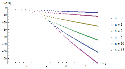
Figure 1: $\ln|U9j|$ vs.$\ln j$ for many values of $n$

We present results of the percent deviation of our approximate values of $3j$ and $U9j$ from the exact values in Tables 3 and 4.

Table 3: Comparison of the exact and asymptotic values of the 3j symbols

	j	Accepted 3j	Approximate 3j	Percent Error
$n=0$
	9/2	0.0917186951	0.0859524287	6.28690401
	99/2	0.0143074760	0.0142302863	0.539505856
	999/2	0.00251476295	0.00251342493	0.0532063347
	9999/2	0.000446679154	0.000446655420	0.00531331215
$n=1$
	9/2	-0.0703281160	-0.0607775452	13.5800180
	99/2	-0.0101817625	-0.0100623320	1.17298491
	999/2	-0.00177932008	-0.00177725981	0.115789693
	9999/2	-0.000315869604	-0.000315833077	0.0115641443
$n=2$
	9/2	0.0667864681	0.0526348981	21.1892774
	99/2	0.00887471327	0.00871423511	1.80826305
	999/2	0.00154190275	0.00153915215	0.178390316
	9999/2	0.000273568204	0.000273519468	0.0178151485
$n=10$
	99/2	0.00642003383	0.00597328117	6.95872744
	999/2	0.00106225244	0.00105503104	0.679819882
	9999/2	0.000187614589	0.000187487331	0.0678293749
$n=100$
	999/2	0.000637437519	0.000596632653	6.40139073
	9999/2	0.000106699870	0.000106026325	0.631251795

Table 4: Comparison of the exact and asymptotic values of the U9j symbols

	j	Accepted U9j	Approximate U9j	Percent Error
$n=0$
	9/2	0.492152957	0.500000000	1.59443179
	99/2	0.499361854	0.500000000	0.127792280
	999/2	0.499937371	0.500000000	0.0125274006
	9999/2	0.499993749	0.500000000	0.00125027349
$n=1$
	9/2	-0.0378955625	-0.0340206909	10.2251328
	99/2	-0.00312046463	-0.00309279008	0.886872805
	999/2	-0.000306761485	-0.000306492711	0.0876166329
	9999/2	-0.0000306243639	-0.0000306216840	0.00875116429
$n=2$
	9/2	0.00606563844	0.00448261961	26.0981402
	99/2	0.0000379552583	0.0000370464431	2.39443810
	999/2	$3.64686293*10^{-7}$	$3.63819464*10^{-7}$	0.237691695
	9999/2	$3.63251097*10^{-9}$	$3.63164818*10^{-9}$	0.0237519144
$n=10$
	99/2	$7.33668833*10^{-17}$	$5.24669432*10^{-17}$	28.4868855
	999/2	$4.95097802*10^{-27}$	$4.79272848*10^{-27}$	3.19632873
	9999/2	$4.76517144*10^{-37}$	$4.74976392*10^{-37}$	0.323335927
$n=20$
	99/2	$1.75313503*10^{-27}$	$5.21781167*10^{-28}$	70.2372517
	999/2	$4.88682624*10^{-48}$	$4.35394087*10^{-48}$	10.9045287
	9999/2	$4.32566*10^{-68}$	$4.27622870*10^{-68}$	1.143

We note other work on asymptotics of CG coefficients by Reinsch and Morehead [3]. In their work they define

$$\beta=((j_{1}+j_{2}-j)(j+j_{2}-j_{1})(j+j_{1}-j_{2})(j_{1}+j_{2}+j))^{1/2}$$ (20)

They find an approximate expression for the CG coeffecients in their Eq.(B9).

$$CG=\left<j_{1}j_{2}00|j0\right>\approx 2(-1)^{\frac{j_{1}+j_{2}-j}{2}}\sqrt{\dfrac{2j+1}{2\pi\beta}}\sqrt{\dfrac{j+j_{1}+j_{2}}{j+j_{1}+j_{2}+1}}(1+\delta_{4}+\delta_{6})$$

$$\times\left[1+\dfrac{1}{24}\left(\dfrac{2}{j}+\dfrac{2}{j_{1}}+\dfrac{1}{j_{2}}-\dfrac{1}{j+j_{1}+j_{2}}-\dfrac{1}{-j+j_{1}+j_{2}}-\dfrac{1}{j-j_{1}+j_{2}}-\dfrac{1}{j+j_{1}-j_{2}}\right)\right]$$ (21)

We quickly run into trouble in making a comparison with our results, especially for $n=0$. In their Eq.(B12) they have in the leading term CG proportional to $\dfrac{1}{\sqrt{\beta}}$. However for the case $j=j_{1}+j_{2}$, that is to say $I=I_{max}$, with our $n=0$, we see that $\beta$ vanishes and hence their expression for CG blows up. Evidently their formula is not valid in this region. On the other hand, our expression Eq. (13) from [1] works just fine.

In this work, we have given the details of how the asymptotic behaviors of selected $3j$ and $9j$ coefficients and their unitary counterparts are obtained. There are some subtleties, e.g. in the second column of Table 1, although term-by-term we get non-zero results, the entire sum is zero and so we must expand further as in the following column. There are similar points for Table 2. We further note that one can take asymptotic limits in more than one way. Here the emphasis is on when the total angular momentum $I$ is large ($I=I_{max}-2n,n\ll j$), and one obtains a power-law behavior $1/j^{n}$ . This is most easily seen by plotting $\ln|U9j|\text{ vs.}\ln j$. On the other hand, if one keeps $I$ fixed and increases $j$ one gets a dominantly exponential behavior, as shown in Eq. (19).This is most easily seen by plotting $U9j$ vs. $j$. Lastly, we recall the physics motivation for this work—how maximum-$j$ pairing manifests itself in nuclei [5].

Brian Kleszyk thanks the Rutgers Aresty Research Center for Undergraduates for support during the 2013-2014 academic year. Daniel Hertz-Kintish also thanks the Rutgers Aresty Research Center for Undergraduates for support during the 2014 summer session.

- [1] B. Kleszyk and L. Zamick, Analytical and Numerical Calculations for the Asymptotic Behaviors of Unitary Coefficients Phys. Rev C.89.044322 (2014)
- [2] G. Racah, Phys. Rev. 62, 438 (1942)
- [3] M.W. Reinsch and J.J. Morehead, Journal of Mathematical Physics 40, 4782 (1999)
- [4] D. A. Varshalovich, A. N. Moskalev, V. K. Khersonskii, Quantum Theory of Angular Momentum, World Scientific, Singapore (1988)
- [5] L. Zamick and A. Escuderos, Phys. Rev. C.87.044302 (2013)