Multi-level higher order QMC Galerkin discretization for
affine parametric operator equations

Abstract

We develop a convergence analysis of a multi-level algorithm combining higher order quasi-Monte Carlo (QMC) quadratures with general Petrov-Galerkin discretizations of countably affine parametric operator equations of elliptic and parabolic type, extending both the multi-level first order analysis in [F.Y. Kuo, Ch. Schwab, and I.H. Sloan, Multi-level quasi-Monte Carlo finite element methods for a class of elliptic partial differential equations with random coefficient (Found. Comp. Math., 2015)] and the single level higher order analysis in [J. Dick, F.Y. Kuo, Q.T. Le Gia, D. Nuyens, and Ch. Schwab, Higher order QMC Galerkin discretization for parametric operator equations (SIAM J. Numer. Anal., 2014)]. We cover, in particular, both definite as well as indefinite, strongly elliptic systems of partial differential equations (PDEs) in non-smooth domains, and discuss in detail the impact of higher order derivatives of Karhunen-Loève eigenfunctions in the parametrization of random PDE inputs on the convergence results. Based on our a-priori error bounds, concrete choices of algorithm parameters are proposed in order to achieve a prescribed accuracy under minimal computational work. Problem classes and sufficient conditions on data are identified where multi-level higher order QMC Petrov-Galerkin algorithms outperform the corresponding single level versions of these algorithms. Numerical experiments confirm the theoretical results.

1 Introduction

The efficient numerical computation of statistical quantities for solutions of partial differential and of integral equations with random inputs is a key task in uncertainly quantification and in the sciences. In this paper, we combine the use of higher order quasi-Monte Carlo (QMC) quadrature with Petrov-Galerkin discretization in a multi-level algorithm to estimate a quantity of interest which has been expressed as an infinite dimensional integral. This paper applies the new QMC theory developed in [8] (for a single level algorithm) to the QMC Finite Element multi-level algorithm introduced in [23], to yield a potentially reduced exponent $a$ in the cost bound of $\mathcal{O}(\varepsilon^{-a})$, subject to a fixed error threshold $\varepsilon>0$, with the constant implied in $\mathcal{O}(\cdot)$ being independent of the dimension of the integration domain.

The multi-level algorithm has first been introduced in [17] in the context of integral equations and was independently rediscovered in [12] in the context of simulation of stochastic differential equations. A combination of the multi-level approach with the Monte Carlo method has recently been developed for elliptic problems with random input data in [1, 3, 2, 16, 33, 5].

Let ${\boldsymbol{y}}:=(y_{j})_{j\geq 1}$ denote the possibly countable set of parameters from a domain $U\subseteq\mathbb{R}^{\mathbb{N}}$, and let $A({\boldsymbol{y}})$ denote a ${\boldsymbol{y}}$-parametric bounded linear operator between suitably defined spaces $\mathcal{X}$ and $\mathcal{Y}^{\prime}$. We consider parametric operator equations: given $f\in\mathcal{Y}^{\prime}$, for every ${\boldsymbol{y}}\in U$ find $u({\boldsymbol{y}})\in\mathcal{X}$ such that

$$A({\boldsymbol{y}})\,u({\boldsymbol{y}})=f\;.$$ (1)

Such parametric operator equations arise from partial differential equations with random field input, see, e.g., [29] and the references there. Following [28, 8], we consider in this paper problems where $A({\boldsymbol{y}})$ has “affine” parameter dependence, i.e., there exists a sequence $\{A_{j}\}_{j\geq 0}\subset\mathcal{L}(\mathcal{X},\mathcal{Y}^{\prime})$ such that for every ${\boldsymbol{y}}\in U$ we can write

$$A({\boldsymbol{y}})=A_{0}+\sum_{j\geq 1}y_{j}\,A_{j}\;,$$ (2)

and we restrict ourselves to the bounded (infinite-dimensional) parameter domain

$${U=[-\tfrac{1}{2},\tfrac{1}{2}]^{\mathbb{N}}}\;.$$

Some assumptions on the “nominal” (or “mean field”) operator $A_{0}$ and the “fluctuation” operators $A_{j}$ are required to ensure that the sum in (2) converges, and to ensure its well-posedness, i.e., the existence and uniqueness of the parametric solution $u({\boldsymbol{y}})$ in (1) for all ${\boldsymbol{y}}\in U$; sufficient conditions will be specified in §2. Further assumptions on $A_{0}$ and $A_{j}$ are required for our regularity and approximation results; these will also be given in §2. For now we mention only one key assumption: there exists $\bar{t}\geq 0$ such that for every $0\leq t\leq\bar{t}$ there exists a $0<p_{t}<1$ for which

$$\sum_{j\geq 1}\|A_{j}\|_{\mathcal{L}(\mathcal{X}_{t},\mathcal{Y}^{\prime}_{t})}^{p_{t}}\,<\,\infty\qquad\mbox{and}\qquad\sum_{j\geq 1}\|A_{j}^{*}\|_{\mathcal{L}(\mathcal{Y}_{t},\mathcal{X}^{\prime}_{t})}^{p_{t}}\,<\,\infty\;,$$ (3)

where $\{\mathcal{X}_{t}\}_{t\geq 0}$ and $\{\mathcal{Y}_{t}\}_{t\geq 0}$ denote scales of smoothness spaces (see (18) ahead), with $\mathcal{X}_{0}=\mathcal{X}$ and $\mathcal{Y}_{0}=\mathcal{Y}$, and $\|\cdot\|_{\mathcal{L}(\mathcal{X}_{t},\mathcal{Y}^{\prime}_{t})}$ denotes the operator norm for the set of all bounded linear mappings from $\mathcal{X}_{t}$ to $\mathcal{Y}^{\prime}_{t}$. As we will explain, it is natural to assume that $0<p_{0}\leq p_{1}\leq\cdots\leq p_{\bar{t}}<1$. Assumption (3) implies a decay of the fluctuations $A_{j}$ in (2), with stronger decay as the value of $p_{0}$ decreases.

For a quantity of interest (or “goal” functional) $G\in\mathcal{X}^{\prime}$, “ensemble averages” of all possible realizations of the operator equation (1) take the form of an integral over $U$,

$$I(G(u))\,:=\,\int_{U}G(u({\boldsymbol{y}}))\,{\mathrm{d}}{\boldsymbol{y}}\;.$$ (4)

This calls for the consideration of QMC methods for numerical integration. A single level QMC strategy was developed and analyzed in [21], and subsequently generalized and improved in [28, 8]. It contained three approximations: (i) dimension-truncating the infinite sum in (2) to $s$ terms (see §2.5), (ii) solving the corresponding operator equation (1) using a Finite Element method, or more generally, Petrov-Galerkin discretization based on two dense, one-parameter families $\{\mathcal{X}^{h}\}_{h>0}\subset\mathcal{X}$, $\{\mathcal{Y}^{h}\}_{h>0}\subset\mathcal{Y}$ of finite dimensional subspaces (see §2.4), and (iii) approximating the corresponding integral (4) using a QMC rule with $N$ points in $s$ dimensions. Thus (4) was approximated by

$$Q_{s,N}(G(u^{h}_{s})):=\frac{1}{N}\sum_{n=0}^{N-1}G\big{(}u^{h}_{s}\big{(}{{\boldsymbol{y}}_{n}-{\bf\tfrac{1}{2}}}\big{)}\big{)}\;,$$ (5)

where $\{{\boldsymbol{y}}_{0},\ldots,{\boldsymbol{y}}_{N-1}\}\subset[0,1]^{s}$ are $N$ suitably chosen QMC points, and the shift of coordinates by ${\textstyle\boldsymbol{\frac{1}{2}}}$ in (5) accounts for the translation from $[0,1]^{s}$ to $[-\frac{1}{2},\frac{1}{2}]^{s}$.

In [21], first order QMC methods known as randomly shifted lattice rules were considered, together with first order finite element methods, to achieve an overall root-mean-square error bound (with respect to the random shift) of

$$\mbox{r.m.s.\ error}\,=\,\mathcal{O}\left(s^{-2(1/p_{0}-1)}+N^{-\min(1/p_{0}-1/2,1-\delta)}+h^{t+t^{\prime}}\right),\quad\delta>0\;,$$ (6)

for a second order, elliptic PDE in the bounded spatial domain $D\subset\mathbb{R}^{d}$,

$$-\nabla\cdot\left(a({\boldsymbol{y}})\nabla u({\boldsymbol{y}})\right)\,=\,f\;,\quad u({\boldsymbol{y}})|_{\partial D}=0\;,\quad a({\boldsymbol{y}})\,=\,a_{0}(\cdot)+\sum_{j\geq 1}y_{j}\,\psi_{j}(\cdot)\;,$$ (7)

which corresponds to the special case with $\mathcal{X}=\mathcal{Y}=H^{1}_{0}(D)$, where $0<p_{0}<1$, $0\leq t,t^{\prime}\leq 1$, $f\in H^{-1+t}(D)$ and $G\in H^{-1+t^{\prime}}(D)$. The result is then generalized in [28] to the general affine family of operator equations. The implied constant in the bound (6) and the QMC convergence rate with respect to $N$ are independent of the integration dimension $s$, and this is achieved by choosing appropriate “product and order dependent $($POD$)$ weights” in the function space setting for the QMC analysis. A suitable generating vector for the required lattice rule can be constructed using a component-by-component (CBC) algorithm, at a (pre-computation) cost of $\mathcal{O}(s\,N\log N+s^{2}N)$ operations.

The QMC convergence rate in (6) was capped at order one in [21, 28], but this limitation was overcome in [8] by considering a family of higher order digital nets known as (deterministic) interlaced polynomial lattice rules, together with higher order Galerkin discretization, to achieve an error bound of

$$\mbox{error}\,=\,\mathcal{O}\left(s^{-2(1/p_{0}-1)}+N^{-1/p_{0}}+h^{t+t^{\prime}}\right),$$ (8)

for $0<p_{0}<1$, $0\leq t,t^{\prime}\leq\bar{t}$, $f\in\mathcal{Y}_{t}^{\prime}$ and $G\in\mathcal{X}^{\prime}_{t^{\prime}}$. The QMC convergence rate proved in [8] also gained an additional factor of $N^{-1/2}$ as compared to the rate for randomly shifted lattice rules in [21, 28], thanks to a new, non-Hilbert space setting for the QMC analysis (proposed already in [22]). This approach is outlined in §2.6. The implied constant in (8) is again independent of $s$, and this time it is achieved by choosing appropriate “smoothness driven product and order dependent $($SPOD$)$ weights” for the function space. The generating vector for the required interlaced polynomial lattice rule can again be constructed using a CBC algorithm, at a slightly higher cost of $\mathcal{O}(\alpha\,s\,N\log N+\alpha^{2}\,s^{2}N)$ operations, with $\alpha=\lfloor 1/p_{0}\rfloor+1\geq 2$.

To reduce the computational cost required to achieve the same error, a novel multi-level algorithm was introduced and analyzed in [23]. It takes the form

$$Q^{L}_{*}(G(u))\,:=\,\sum_{\ell=0}^{L}Q_{s_{\ell},N_{\ell}}(G(u^{h_{\ell}}_{s_{\ell}}-u^{h_{\ell-1}}_{s_{\ell-1}}))\;,$$ (9)

where each $Q_{s_{\ell},N_{\ell}}$ is a randomly shifted lattice rule with $N_{\ell}$ points in $s_{\ell}$ dimensions, and where $u^{h_{-1}}_{s_{-1}}:=0$. The corresponding root-mean-square error bound is

$${\mbox{r.m.s.\ error}\,=\,}$$

$$\mathcal{O}\left(s_{L}^{-2(1/p_{0}-1)}+h_{L}^{t+t^{\prime}}+\sum_{\ell=0}^{L}N_{\ell}^{-\min(1/p_{1}-1/2,1-\delta)}\left(s_{{\ell-1}}^{-(1/p_{0}-1/p_{1})}+h_{{\ell-1}}^{t+t^{\prime}}\right)\right),\quad\delta>0,$$ (10)

where $s_{-1}:=1$, $h_{-1}:=1$, $0<p_{0}\leq p_{1}<1$, $0\leq t,t^{\prime}\leq 1$, and the implied constant is independent of $s$, with appropriately chosen POD weights. Assuming that the overall cost of (9) is $\mathcal{O}(\sum_{\ell=0}^{L}s_{\ell}N_{\ell}h_{\ell}^{-d})$, an argument based on the Lagrange multipliers was used to optimize the choice of $s_{\ell}$ and $N_{\ell}$ in relation to $h_{\ell}\asymp 2^{-\ell}$. Note that the QMC convergence rate with respect to $N_{\ell}$ in (1) depends on $p_{1}$, rather than on $p_{0}$.

In this paper, we replace the randomly shifted lattice rules in (9) by interlaced polynomial lattice rules as in [8], to achieve the improved error bound

$$\mbox{error}\,=\,\mathcal{O}\left(s_{L}^{-2(1/p_{0}-1)}+h_{L}^{t+t^{\prime}}+\sum_{\ell=0}^{L}N_{\ell}^{-1/p_{t}}\left(s_{\ell-1}^{-(1/p_{0}-1/p_{t})}+h_{\ell-1}^{t+t^{\prime}}\right)\right),$$ (11)

where $0<p_{0}\leq p_{t}<1$, $0\leq t,t^{\prime}\leq\bar{t}$. The implied constant is independent of $s$, again, under the provision of appropriate SPOD weights. Comparing (11) with (1), we see that the convergence rate is no longer capped at order one as expected, and there is a gain of the additional factor $N_{\ell}^{-1/2}$ as in (8). However, the convergence rate depends now on the summability exponent $p_{t}$ rather than $p_{0}$ or $p_{1}$.

As we argue in §2.3 of this paper, in many examples, the exponent $p_{t}$ in (3) satisfies

$$p_{t}=\frac{p_{0}}{1-tp_{0}/d},\quad 1\leq t\leq\bar{t}\;,$$ (12)

which could be much larger than $p_{0}$. The requirement $p_{t}<1$ imposes a constraint on $\bar{t}$, the maximum allowable value of $t$ and $t^{\prime}$, which in turn reduces the convergence rate in (11). In some scenarios the potential gain of the multi-level algorithm (9) over the single level algorithm (5) (whose error bound depends only on $p_{0}$) can be limited.

The outline of this paper is as follows. In §2, we formulate the affine parametric operator equations, specify all assumptions which are subsequently needed in our QMC error analysis, and introduce an abstract Petrov-Galerkin discretization of these operator equations which covers most Galerkin discretizations of parabolic and elliptic partial differential equations in a bounded spatial domain $D$. Examples include second order, elliptic divergence form PDEs in polyhedral domains as considered in [25]. We elaborate on (12) resulting from random field modelling with covariance operators chosen as negative powers of second order, elliptic pseudo-differential operators in $D$. We also give in §2 a synopsis of the key results of our single level QMC Petrov-Galerkin error analysis in [8], to the extent required for the present work. In §3, we introduce the multi-level QMC Petrov-Galerkin approximation as direct generalization of the multi-level algorithm based on (first order) randomly shifted lattice rules analyzed in [23]. We present the basic error bounds for the combined QMC Petrov-Galerkin error, refining and extending the analysis of [8], and derive concrete selections of the algorithm parameters based on optimization of the error bounds. The proposed parameter choices are then used to derive asymptotic accuracy versus work bounds for the proposed algorithms, subject to given data regularity in terms of spatial differentiability as well as decay of the covariance spectrum of the random field input. Finally in §5 we give some concluding remarks.

2 Problem formulation

Generalizing results of [4], we study well-posedness, regularity and polynomial approximation of solutions for a family of abstract parametric saddle point problems, with operators depending on a sequence of parameters. The results cover a wide range of affine parametric operator equations: among them are stationary and time-dependent diffusion in random media [4], wave propagation [19], and optimal control problems for uncertain systems [20].

2.1 Affine parametric operator equations

We denote by $\mathcal{X}$ and $\mathcal{Y}$ two separable and reflexive Banach spaces over $\mathbb{R}$ (all results will hold with the obvious modifications also for spaces over $\mathbb{C}$) with (topological) duals $\mathcal{X}^{\prime}$ and $\mathcal{Y}^{\prime}$, respectively. By $\mathcal{L}(\mathcal{X},\mathcal{Y}^{\prime})$, we denote the set of bounded linear operators $A:\mathcal{X}\to\mathcal{Y}^{\prime}$.

A particular instance of (1) and (2) are boundary value problems of second order, elliptic (systems of) partial differential equations such as linear elasticity in anisotropic, parametric medium. Here, $\mathcal{X}=\mathcal{Y}=H^{1}_{0}(D)^{\iota}$ with $\iota\geq 1$, and $A({\boldsymbol{y}})$ is given by the divergence-form elliptic differential operator which acts on vector functions $u({\boldsymbol{y}}):D\mapsto{\mathbb{R}}^{\iota}$ via

$$(A({\boldsymbol{y}})u({\boldsymbol{y}}))_{l}\,=\,-\sum_{i,j=1}^{d}\sum_{k=1}^{\iota}\partial_{i}(a^{ij}_{kl}({\boldsymbol{x}},{\boldsymbol{y}})\partial_{j}u_{k}({\boldsymbol{x}},{\boldsymbol{y}}))\,=\,f_{l}\quad\mbox{in}\quad D,\;l=1,...,\iota,$$ (13)

and $u({\boldsymbol{y}})|_{\partial D}=0$. In the scalar, isotropic case of (13) which was considered in [21], we have $\iota=1$ and the coefficient function $a^{ij}({\boldsymbol{y}})=\delta_{ij}a({\boldsymbol{y}})$ with $a({\boldsymbol{y}})$ as in (7). For linearized elasticity, $\iota=d$ in (13). Other boundary conditions in (13) could equally well be considered (we refer to [25, Sec.1.2] for details).

As we explained in the introduction, let ${\boldsymbol{y}}:=(y_{j})_{j\geq 1}\in U=[-\frac{1}{2},\frac{1}{2}]^{\mathbb{N}}$ be a countable set of parameters. For every $f\in\mathcal{Y}^{\prime}$ and for every ${\boldsymbol{y}}\in U$, we solve the parametric operator equation (1), where the operator $A({\boldsymbol{y}})\in\mathcal{L}(\mathcal{X},\mathcal{Y}^{\prime})$ is of affine parameter dependence, see (2). We associate with the operators $A_{j}$ the parametric bilinear forms ${\mathfrak{a}}_{j}(\cdot,\cdot):\mathcal{X}\times\mathcal{Y}\rightarrow\mathbb{R}$ via

$$\forall v\in\mathcal{X},\;w\in\mathcal{Y}:\quad{\mathfrak{a}}_{j}(v,w)\,=\,{{}_{\mathcal{Y}^{\prime}}}\langle A_{j}v,w\rangle_{\mathcal{Y}}\;,\quad j=0,1,2,\ldots\;.$$

Similarly, for ${\boldsymbol{y}}\in U$ we associate with the parametric operator $A({\boldsymbol{y}})$ the parametric bilinear form ${\mathfrak{a}}({\boldsymbol{y}};\cdot,\cdot):\mathcal{X}\times\mathcal{Y}\to\mathbb{R}$ via

$$\forall v\in\mathcal{X},\;w\in\mathcal{Y}:\quad{\mathfrak{a}}({\boldsymbol{y}};v,w)\,=\,{{}_{\mathcal{Y}^{\prime}}}\langle A({\boldsymbol{y}})v,w\rangle_{\mathcal{Y}}\;.$$

In order for the sum in (2) to converge, we impose the assumptions below on the sequence $\{A_{j}\}_{j\geq 0}\subset\mathcal{L}(\mathcal{X},\mathcal{Y}^{\prime})$.

Assumption 1.

The sequence $\{A_{j}\}_{j\geq 0}\subset\mathcal{L}(\mathcal{X},\mathcal{Y}^{\prime})$ in (2) satisfies:

1. $A_{0}\in\mathcal{L}(\mathcal{X},\mathcal{Y}^{\prime})$ is boundedly invertible, i.e., there exists a constant $\mu_{0}>0$ such that

   $$\inf_{0\neq v\in\mathcal{X}}\sup_{0\neq w\in\mathcal{Y}}\frac{{\mathfrak{a}}_{0}(v,w)}{\|v\|_{\mathcal{X}}\|w\|_{\mathcal{Y}}}\geq\mu_{0}\;,\quad\inf_{0\neq w\in\mathcal{Y}}\sup_{0\neq v\in\mathcal{X}}\frac{{\mathfrak{a}}_{0}(v,w)}{\|v\|_{\mathcal{X}}\|w\|_{\mathcal{Y}}}\geq\mu_{0}\;.$$ (14)

2. The fluctuation operators $\{A_{j}\}_{j\geq 1}$ are small with respect to $A_{0}$ in the following sense: there exists a constant $0<\kappa<2$ such that

   $$\sum_{j\geq 1}\beta_{0,j}\leq\kappa<2\;,\quad\mbox{where}\quad\beta_{0,j}\,:=\,\|A_{0}^{-1}A_{j}\|_{\mathcal{L}(\mathcal{X},\mathcal{X})}\;,\quad j=1,2,\ldots\;.$$ (15)

Theorem 1 (cp. [28, Theorem 2]).

Under Assumption 1, for every realization ${\boldsymbol{y}}\in{U}$ of the parameter vector, the affine parametric operator $A({\boldsymbol{y}})$ given by (2) is boundedly invertible, uniformly with respect to ${\boldsymbol{y}}$. In particular, for every $f\in\mathcal{Y}^{\prime}$ and for every ${\boldsymbol{y}}\in{U}$, the parametric operator equation

$$\mbox{find}\quad u({\boldsymbol{y}})\in\mathcal{X}:\quad{\mathfrak{a}}({\boldsymbol{y}};u({\boldsymbol{y}}),w)\,=\,{{}_{\mathcal{Y}^{\prime}}}\langle f,w\rangle_{\mathcal{Y}}\quad\forall w\in\mathcal{Y}$$ (16)

admits a unique solution $u({\boldsymbol{y}})$ which satisfies the a-priori estimate

$$\|u({\boldsymbol{y}})\|_{\mathcal{X}}\,\leq\,\frac{1}{\mu}\,\|f\|_{\mathcal{Y}^{\prime}}\;,\quad\mbox{with}\quad\mu=(1-\kappa/2)\,\mu_{0}\;.$$

2.2 Parametric and spatial regularity of solutions

First we establish the regularity of the solution $u({\boldsymbol{y}})$ of the parametric, variational problem (16) with respect to the parameter vector ${\boldsymbol{y}}$. In the following, let $\mathbb{N}_{0}^{\mathbb{N}}$ denote the set of sequences ${\boldsymbol{\nu}}=(\nu_{j})_{j\geq 1}$ of non-negative integers $\nu_{j}$, and let $|{\boldsymbol{\nu}}|:=\sum_{j\geq 1}\nu_{j}$. For $|{\boldsymbol{\nu}}|<\infty$, we denote the partial derivative of order ${\boldsymbol{\nu}}$ of $u({\boldsymbol{y}})$ with respect to ${\boldsymbol{y}}$ by

$$\partial^{\boldsymbol{\nu}}_{\boldsymbol{y}}u({\boldsymbol{y}})\,:=\,\frac{\partial^{|{\boldsymbol{\nu}}|}}{\partial^{\nu_{1}}_{y_{1}}\partial^{\nu_{2}}_{y_{2}}\cdots}u({\boldsymbol{y}})\;.$$

Theorem 2 (cp. [4, 20]).

Under Assumption 1, there exists a constant $C_{0}>0$ such that for every $f\in\mathcal{Y}^{\prime}$ and for every ${\boldsymbol{y}}\in{U}$, the partial derivatives of the parametric solution $u({\boldsymbol{y}})$ of the parametric operator equation (1) with affine parametric, linear operator (2) satisfy the bounds

$$\|\partial^{\boldsymbol{\nu}}_{\boldsymbol{y}}u({\boldsymbol{y}})\|_{\mathcal{X}}\,\leq\,C_{0}\,|{\boldsymbol{\nu}}|!\,{\boldsymbol{\beta}}_{0}^{\boldsymbol{\nu}}\,\|f\|_{\mathcal{Y}^{\prime}}\quad\mbox{for all }{\boldsymbol{\nu}}\in\mathbb{N}_{0}^{\mathbb{N}}\mbox{ with }|{\boldsymbol{\nu}}|<\infty\;,$$ (17)

where $0!:=1$, ${\boldsymbol{\beta}}_{0}^{\boldsymbol{\nu}}:=\prod_{j\geq 1}\beta_{0,j}^{\nu_{j}}$, with $\beta_{0,j}$ as in (15), and $|{\boldsymbol{\nu}}|=\sum_{j\geq 1}\nu_{j}$.

For the spatial regularity, we assume given scales of smoothness spaces $\{\mathcal{X}_{t}\}_{t\geq 0}$, $\{\mathcal{Y}_{t}\}_{t\geq 0}$, with

$$\mathcal{X} =\mathcal{X}_{0}\supset\mathcal{X}_{1}\supset\mathcal{X}_{2}\supset\cdots\;, \mathcal{Y} =\mathcal{Y}_{0}\supset\mathcal{Y}_{1}\supset\mathcal{Y}_{2}\supset\cdots\;,\quad\mbox{and}$$ (18)

$$\mathcal{X}^{\prime} =\mathcal{X}^{\prime}_{0}\supset\mathcal{X}^{\prime}_{1}\supset\mathcal{X}^{\prime}_{2}\supset\cdots\;, \mathcal{Y}^{\prime} =\mathcal{Y}^{\prime}_{0}\supset\mathcal{Y}^{\prime}_{1}\supset\mathcal{Y}^{\prime}_{2}\supset\cdots\;.$$

The scales are assumed to be defined also for non-integer values of the smoothness parameter $t\geq 0$ by interpolation. For self-adjoint operators, usually $\mathcal{X}_{t}=\mathcal{Y}_{t}$. For example, in diffusion problems in convex domains $D$ considered in [4, 21], the smoothness scales (18) are $\mathcal{X}=\mathcal{Y}=H^{1}_{0}(D)$, $\mathcal{X}_{1}=\mathcal{Y}_{1}=(H^{2}\cap H^{1}_{0})(D)$, $\mathcal{Y}^{\prime}=H^{-1}(D)$, $\mathcal{Y}^{\prime}_{1}=L^{2}(D)$. In a non-convex polygon (or polyhedron), analogous smoothness scales are available, but involve Sobolev spaces with weights. In [25], this kind of abstract regularity result was established for a wide range of second order parametric, elliptic systems in 2D and 3D, also for higher order regularity. The smoothness scales $\{\mathcal{X}_{t}\}_{t\geq 0}$ and $\{\mathcal{Y}^{\prime}_{t}\}_{t\geq 0}$ are then weighted Sobolev spaces $\mathcal{K}^{t+1}_{a+1}(D)$ of Kondratiev type in $D$, and $\mathcal{X}_{t}=\mathcal{K}^{t+1}_{a+1}(D)$, $\mathcal{Y}^{\prime}_{t}=\mathcal{K}^{t-1}_{a-1}(D)$ in this case. The Finite Element spaces which realize the maximal convergence rates (beyond order one) are regular, simplicial families in the sense of Ciarlet, on suitably refined meshes which compensate for the corner and edge singularities.

The maximum amount of smoothness in the scale $\mathcal{X}_{t}$, denoted by $\bar{t}\geq 0$, depends on the problem class under consideration and on the Sobolev scale: e.g., for elliptic problems in polygonal domains, it is well known that choosing for $\mathcal{X}_{t}$ the usual Sobolev spaces will allow (19) with $t$ only in a possibly small interval $0<t\leq\bar{t}$, whereas choosing $\mathcal{X}_{t}$ as Sobolev spaces with weights will allow rather large values of $\bar{t}$ (see, e.g., [25]).

We next formalize the parametric regularity hypothesis.

Assumption 2.

There exists $\bar{t}\geq 0$ such that the following conditions hold:

1. For every $t,t^{\prime}$ satisfying $0\leq t,t^{\prime}\leq\bar{t}$, we have

   $$\sup_{{\boldsymbol{y}}\in{U}}\|A({\boldsymbol{y}})^{-1}\|_{\mathcal{L}(\mathcal{Y}^{\prime}_{t},\mathcal{X}_{t})}<\infty\quad\mbox{and}\quad\sup_{{\boldsymbol{y}}\in{U}}\|(A^{*}({\boldsymbol{y}}))^{-1}\|_{\mathcal{L}(\mathcal{X}^{\prime}_{t^{\prime}},\mathcal{Y}_{t^{\prime}})}<\infty\;.$$ (19)

   Moreover, for every $t$ satisfying $0\leq t\leq\bar{t}$, there exist summability exponents $0\leq p_{0}\leq p_{t}\leq p_{\bar{t}}<1$ such that

   $$\sum_{j\geq 1}\|A_{j}\|^{p_{t}}_{\mathcal{L}(\mathcal{X}_{t},\mathcal{Y}^{\prime}_{t})}<\infty\;.$$ (3)

2. Let ${\boldsymbol{u}}({\boldsymbol{y}})=(A({\boldsymbol{y}}))^{-1}f$ and $w({\boldsymbol{y}})=(A^{*}({\boldsymbol{y}}))^{-1}G$. For $0\leq t,t^{\prime}\leq\bar{t}$, there exist constants $C_{t},C_{t^{\prime}}>0$ such that for every $f\in\mathcal{Y}^{\prime}_{t}$ and $G\in\mathcal{X}^{\prime}_{t^{\prime}}$ holds

   $$\sup_{{\boldsymbol{y}}\in U}\|u({\boldsymbol{y}})\|_{\mathcal{X}_{t}}\leq C_{t}\|f\|_{\mathcal{Y}^{\prime}_{t}}\quad\mbox{and}\quad\sup_{{\boldsymbol{y}}\in U}\|w({\boldsymbol{y}})\|_{\mathcal{Y}_{t^{\prime}}}\leq C_{t^{\prime}}\|G\|_{\mathcal{X}^{\prime}_{t^{\prime}}}\;.$$ (20)

   Moreover, for every $t$ satisfying $0\leq t\leq\bar{t}$, there exists a sequence ${\boldsymbol{\beta}}_{t}=(\beta_{t,j})_{j\geq 1}\in\ell^{p_{t}}(\mathbb{N})$, i.e., satisfying

   $$\sum_{j\geq 1}\beta_{t,j}^{p_{t}}\,<\,\infty\;,$$ (21)

   such that for every $0\leq t,t^{\prime}\leq\bar{t}$ and for every ${\boldsymbol{\nu}}\in\mathbb{N}_{0}^{\mathbb{N}}$ with $|{\boldsymbol{\nu}}|<\infty$ we have

   $$\sup_{{\boldsymbol{y}}\in U}\|\partial^{{\boldsymbol{\nu}}}_{{\boldsymbol{y}}}u({\boldsymbol{y}})\|_{\mathcal{X}_{t}} \,\leq\,C_{t}\,|{\boldsymbol{\nu}}|!\,{\boldsymbol{\beta}}_{t}^{{\boldsymbol{\nu}}}\,\|f\|_{\mathcal{Y}_{t}^{\prime}},$$ (22)

   $$\sup_{{\boldsymbol{y}}\in U}\|\partial^{{\boldsymbol{\nu}}}_{{\boldsymbol{y}}}w({\boldsymbol{y}})\|_{\mathcal{Y}_{t^{\prime}}} \,\leq\,C_{t^{\prime}}\,|{\boldsymbol{\nu}}|!\,{\boldsymbol{\beta}}_{t^{\prime}}^{\boldsymbol{\nu}}\,\|G\|_{\mathcal{X}^{\prime}_{t^{\prime}}}\;.$$ (23)

3. The operators $A_{j}$ are enumerated so that the sequence ${\boldsymbol{\beta}}_{0}$ in (15) satisfies

   $$\beta_{0,1}\geq\beta_{0,2}\geq\cdots\geq\beta_{0,j}\geq\,\cdots\;.$$ (24)

Parametric regularity as in Item 2 of Assumption 2 is available for numerous parametric differential equations (see [29, 18, 15, 20] and the references there) as well as for posterior densities in Bayesian inverse problems with uniform priors (see, e.g., [26, 27] and the references there). Writing $A({\boldsymbol{y}})=A_{0}(I+\sum_{j\geq 1}y_{j}A_{0}^{-1}A_{j})$, a Neumann series argument shows that a sufficient condition for (19) to hold is $A_{0}^{-1}\in\mathcal{L}(\mathcal{Y}^{\prime}_{t},\mathcal{X}_{t})$, $A_{j}\in\mathcal{L}(\mathcal{X}_{t},\mathcal{Y}^{\prime}_{t})$ and that

$$\sum_{j\geq 1}\|A_{0}^{-1}A_{j}\|_{\mathcal{L}(\mathcal{X}_{t},\mathcal{X}_{t})}<2\;.$$

We may estimate

$$\|A_{0}^{-1}A_{j}\|_{\mathcal{L}(\mathcal{X}_{t},\mathcal{X}_{t})}\leq\|A_{0}^{-1}\|_{\mathcal{L}(\mathcal{Y}^{\prime}_{t},\mathcal{X}_{t})}\|A_{j}\|_{\mathcal{L}(\mathcal{X}_{t},\mathcal{Y}^{\prime}_{t})}\;,\;\;j=1,2,3,\cdots\;,$$

and since $A_{j}=A_{0}A_{0}^{-1}A_{j}$ we have $\|A_{j}\|_{\mathcal{L}(\mathcal{X}_{t},\mathcal{Y}^{\prime}_{t})}\leq\|A_{0}\|_{\mathcal{L}(\mathcal{X}_{t},\mathcal{Y}_{t}^{\prime})}\|A_{0}^{-1}A_{j}\|_{\mathcal{L}(\mathcal{X}_{t},\mathcal{X}_{t})}$. Combining these two estimates, we have for every $j\geq 1$

$$\|A_{0}\|_{\mathcal{L}(\mathcal{X}_{t},\mathcal{Y}_{t}^{\prime})}^{-1}\leq\frac{\|A_{0}^{-1}A_{j}\|_{\mathcal{L}(\mathcal{X}_{t},\mathcal{X}_{t})}}{\|A_{j}\|_{\mathcal{L}(\mathcal{X}_{t},\mathcal{Y}^{\prime}_{t})}}\leq\|A_{0}^{-1}\|_{\mathcal{L}(\mathcal{Y}^{\prime}_{t},\mathcal{X}_{t})}\;.$$ (25)

This shows that condition (3) is equivalent to (but not identical to) the condition that $\sum_{j\geq 1}\|A_{0}^{-1}A_{j}\|^{p_{t}}_{\mathcal{L}(\mathcal{X}_{t},\mathcal{X}_{t})}<\infty$.

2.3 Illustration of Assumption 2

The condition (14) of Assumption 1 implies $A_{0}^{-1}\in\mathcal{L}(\mathcal{Y}^{\prime},\mathcal{X})$ so that for every ${\boldsymbol{y}}\in U$ we have $A({\boldsymbol{y}})\,u({\boldsymbol{y}})=f\Longleftrightarrow B({\boldsymbol{y}})\,u({\boldsymbol{y}})=\tilde{f}$, where $B({\boldsymbol{y}}):=I+\sum_{j\geq 1}y_{j}(A_{0}^{-1}A_{j})$ and $\tilde{f}:=A_{0}^{-1}f$. Taking ${\boldsymbol{y}}={\boldsymbol{0}}$ in (19) yields $A_{0}^{-1}\in\mathcal{L}(\mathcal{Y}^{\prime}_{t},\mathcal{X}_{t})$, while (3) and (25) together gives $A_{0}^{-1}A_{j}\in\mathcal{L}(\mathcal{X}_{t},\mathcal{X}_{t})$ for $j=1,2,\ldots$. Hence (21) holds with $\beta_{t,j}:=\|A_{0}^{-1}A_{j}\|_{\mathcal{L}(\mathcal{X}_{t},\mathcal{X}_{t})}$. We may now apply the argument in [4] to the affine parametric operator equation $B({\boldsymbol{y}})u({\boldsymbol{y}})=\tilde{f}$ to obtain (22). Repeating this argument for the adjoint equation $B({\boldsymbol{y}})^{*}w({\boldsymbol{y}})=\tilde{G}:=A_{0}^{-*}G\in\mathcal{X}_{t}$ then yields (23).

The summability (21) is well known to be related to the smoothness of the covariance kernels of the random coefficient; see e.g., [30, Appendix] for details. We illustrate (21) in the context of the scalar, parametric diffusion problem (7). One source of the $\psi_{j}$ in (7) are principal component analysis expansions such as Karhunen-Loève expansions of random coefficients, and therefore (21) is a sparsity assumption on the coefficient function sequence $\{\psi_{j}\}_{j\geq 1}$ and their derivatives of orders $t=1,2,\ldots,\lfloor\bar{t}\rfloor$.

Consider the Dirichlet Laplacean $-\Delta_{d}$ in the unit cube $D=(0,1)^{d}$ with $d\geq 1$. This is an unbounded, self-adjoint operator on $L^{2}(D)$ with a discrete spectrum consisting of countably many real eigenvalues which accumulate only at infinity. It is elementary to verify by separation of variables that the eigenpairs of $-\Delta_{d}$ are

$$-\Delta_{d}\,\tilde{\psi}_{{\boldsymbol{k}}}\,=\,\lambda_{{\boldsymbol{k}}}\,\tilde{\psi}_{{\boldsymbol{k}}}\quad\mbox{in}\quad D,\quad\tilde{\psi}_{{\boldsymbol{k}}}|_{\partial D}=0\;,\quad{\boldsymbol{k}}=(k_{1},\ldots,k_{d})\in\mathbb{N}^{d}\;,$$

with

$$\lambda_{{\boldsymbol{k}}}\,=\,\pi^{2}(k_{1}^{2}+\cdots+k_{d}^{2}),\;\;\tilde{\psi}_{{\boldsymbol{k}}}({\boldsymbol{x}})\,=\,\prod_{i=1}^{d}\sin(\pi k_{i}x_{i})\;.$$ (26)

Enumerating $\{\lambda_{{\boldsymbol{k}}}\}_{{\boldsymbol{k}}\in\mathbb{N}^{d}}$ in non-decreasing order $\{\lambda_{j}\}_{j\geq 1}$, there hold the Weyl asymptotics (see, e.g., [31] and the references there)

$$\lambda_{j}\sim j^{2/d}\quad\mbox{as}\quad j\to\infty\;.$$ (27)

Next, we consider again the domain $D$, but now for some real parameter $\theta>0$ the Covariance operator $\mathcal{C}_{\theta}=(-\Delta_{d})^{-\theta}$. Then, for any $\theta>0$, $\mathcal{C}_{\theta}\in\mathcal{L}(L^{2}(D),L^{2}(D))$ is a compact, self-adjoint operator whose spectrum $\sigma(\mathcal{C}_{\theta})=(\mu_{j})_{j\geq 1}$ consists of countably many, real eigenvalues which we enumerate again in non-increasing order. By the spectral mapping theorem and the Weyl asymptotics (27), the operators $\mathcal{C}_{\theta}$ have the same eigenfunctions $\tilde{\psi}_{j}$ as the operator $-\Delta_{d}$, and the corresponding eigenvalues $\mu_{j}$ of $\mathcal{C}_{\theta}$ have the asymptotics

$$\mu_{j}\sim j^{-2\theta/d}\quad\mbox{as}\quad j\to\infty\;.$$

In Karhunen-Loève expansions with uncertain coefficients, we have (7) with $\psi_{j}:=\sqrt{\mu_{j}}\,\tilde{\psi}_{j}$. Clearly in this case we have $\|\tilde{\psi}_{j}\|_{L^{\infty}(D)}\leq 1$ for $j\geq 1$, which yields $\|\psi_{j}\|_{L^{\infty}(D)}\lesssim j^{-\theta/d}$, from which we conclude that

$$\sum_{j\geq 1}\|\psi_{j}\|_{L^{\infty}(D)}^{p_{0}}\,<\,\infty\quad\mbox{with}\quad p_{0}\,>\,\frac{d}{\theta}\;.$$

We find for $t=0,1,2,...$ and for every $j\in\mathbb{N}$ that $\|\tilde{\psi}_{j}\|_{W^{t,\infty}(D)}\lesssim j^{{t/d}}$, and therefore

$$\|\psi_{j}\|_{W^{t,\infty}(D)}\lesssim j^{{(t-\theta)/d}}\;,$$ (28)

with the implied constant depending on $t$, but independent of $j\in\mathbb{N}$. So it holds

$$\sum_{j\geq 1}\|\psi_{j}\|_{W^{t,\infty}(D)}^{p_{t}}<\infty\;,\quad\mbox{with}\quad p_{t}\,:=\,\frac{p_{0}}{1-tp_{0}/d}\,<\,\frac{d}{\theta-t}\;.$$

The requirement that $p_{t}<1$ means

$$\bar{t}=d\left(\frac{1}{p_{0}}-1\right)<\theta-d\;.$$

Thus sparsity of expansions of higher order $t$ is only available for sufficiently large $\theta>0$, at least in this example where (28) is sharp.

The preceding arguments rely strongly on the explicit formulas (26). For covariance operators of the form $\mathcal{C}=B^{-\theta}$ for a general, positive and second order, self-adjoint elliptic divergence form partial differential operator $B\in\mathcal{L}(\mathcal{X},\mathcal{X}^{\prime})$ with non-constant, Hölder regular coefficients in a polygonal/polyhedral domain $D$, the spectral asymptotics of the $\lambda_{j}$ as $j\to\infty$ is well known to hold as well (see e.g. [31, Theorem 15.2] for smooth domains and smooth coefficients, and [24] for elliptic, divergence-form operators with non-smooth coefficients). Importantly, also in this case, the eigenfunctions $\tilde{\psi}_{j}$ are bounded, but may exhibit singularities at corners and edges of the domain $D$, so that they belong only to weighted $W^{t,\infty}(D)$ spaces denoted in [25] by $\mathcal{W}^{t,\infty}(D)$; coefficients in such spaces for (13) are admissible in the results of [25], cp. [25, Eq. (2.3)], where also conditions (22) and (23) have been verified for parametric, elliptic systems (13). In the context of the parametric, second-order, elliptic divergence-form PDE (13), we have $\|A_{j}\|_{\mathcal{L}(\mathcal{X}_{t},\mathcal{Y}_{t}^{\prime})}\lesssim\|\psi_{j}\|_{\mathcal{W}^{j,\infty}(D)}$ (cp. [25, Eq. (2.6)]) and $\|A_{0}^{-1}\|_{\mathcal{L}(\mathcal{Y}^{\prime}_{t},\mathcal{X}_{t})}$ being bounded in a scale of weighted Sobolev spaces (cp. [25, Corollary 2.1] with the identification $\mathcal{X}_{t}={\cal K}^{1+t}_{a+1}(D)$), with $\lesssim$ denoting an absolute constant (depending on $t$, but not on $j$); we refer to [25, Eq.(2.6)] for details.

2.4 Petrov-Galerkin discretization

Since the exact solution is not available explicitly, we will have to compute, for given ${\boldsymbol{y}}\in{U}$, an approximate solution obtained by Petrov-Galerkin discretization.

Theorem 3 (cp. [8, §2.4]).

Let $\{\mathcal{X}^{h}\}_{h>0}\subset\mathcal{X}$ and $\{\mathcal{Y}^{h}\}_{h>0}\subset\mathcal{Y}$ be two families of finite dimensional subspaces which are dense in $\mathcal{X}$ and in $\mathcal{Y}$, respectively. Assume moreover the approximation property and that the Petrov-Galerkin subspace pairs $\mathcal{X}^{h}\times\mathcal{Y}^{h}$ are inf-sup stable with respect to the nominal bilinear form ${\mathfrak{a}}_{0}(\cdot,\cdot)$, as in (14), with constant $\bar{\mu}_{0}>0$ independent of $h$. This implies the discrete inf-sup conditions for the bilinear form ${\mathfrak{a}}({\boldsymbol{y}};\cdot,\cdot)$, uniformly with respect to ${\boldsymbol{y}}\in U$, with constant $\bar{\mu}\,=\,(1-\kappa/2)\,\bar{\mu}_{0}>0$.

Then for every ${\boldsymbol{y}}\in U$ we have existence, uniqueness and (uniform with respect to ${\boldsymbol{y}}$) quasioptimality of the Petrov-Galerkin solutions, ie., for every $0<h\leq h_{0}$ and for every ${\boldsymbol{y}}\in{U}$, the Petrov-Galerkin approximations $u^{h}({\boldsymbol{y}})\in\mathcal{X}^{h}$, given by

$$\mbox{find}\;u^{h}({\boldsymbol{y}})\in\mathcal{X}^{h}:\quad{\mathfrak{a}}({\boldsymbol{y}};u^{h}({\boldsymbol{y}}),w^{h})={{}_{\mathcal{Y}^{\prime}}}\langle f,w^{h}\rangle_{\mathcal{Y}}\quad\forall w^{h}\in\mathcal{Y}^{h}\;,$$ (29)

are well defined, and stable, i.e., they satisfy the uniform a-priori estimate

$$\|u^{h}({\boldsymbol{y}})\|_{\mathcal{X}}\,\leq\,\frac{1}{\bar{\mu}}\,\|f\|_{\mathcal{Y}^{\prime}}\;.$$ (30)

Moreover, for $0<t\leq\bar{t}$, if the basis functions have smoothness degree $\lceil t\rceil$ then there exists a constant $C_{t}>0$ such that for every ${\boldsymbol{y}}\in U$

$$\|u({\boldsymbol{y}})-u^{h}({\boldsymbol{y}})\|_{\mathcal{X}}\,\leq\,C_{t}\,h^{t}\,\|u({\boldsymbol{y}})\|_{\mathcal{X}_{t}}\;.$$ (31)

Additionally, we assume uniform inf-sup stability of the pairs $\mathcal{X}^{h}\times\mathcal{Y}^{h}$ for the adjoint problem, so that for $0<t^{\prime}\leq\bar{t}$ there exists a constant $C_{t^{\prime}}>0$ such that for all $0<h\leq h_{0}$ and ${\boldsymbol{y}}\in U$,

$$\|w({\boldsymbol{y}})-w^{h}({\boldsymbol{y}})\|_{\mathcal{Y}}\,\leq\,C_{t^{\prime}}h^{t^{\prime}}\|w({\boldsymbol{y}})\|_{\mathcal{Y}_{t^{\prime}}}\;.$$ (32)

Then, for every $f\in\mathcal{Y}^{\prime}_{t}$ and $G\in\mathcal{X}^{\prime}_{t^{\prime}}$ with $0<t,t^{\prime}\leq\bar{t}$ and for every ${\boldsymbol{y}}\in{U}$, as $h\to 0$, there exists a constant $C>0$ independent of $h>0$ and of ${\boldsymbol{y}}\in U$ such that the Galerkin approximations $G(u^{h}({\boldsymbol{y}}))$ satisfy

$$\left|G(u({\boldsymbol{y}}))-G(u^{h}({\boldsymbol{y}}))\right| \,\leq\,C\,h^{t+t^{\prime}}\,\|f\|_{\mathcal{Y}^{\prime}_{t}}\,\|G\|_{\mathcal{X}^{\prime}_{t^{\prime}}}\;.$$ (33)

2.5 Dimension truncation

We truncate the infinite sum in (2) to $s$ terms and solve the corresponding operator equation (1) approximately using Galerkin discretization from two dense, one-parameter families $\{\mathcal{X}^{h}\}\subset\mathcal{X}$, $\{\mathcal{Y}^{h}\}\subset\mathcal{Y}$ of subspaces of $\mathcal{X}$ and $\mathcal{Y}$: for $s\in\mathbb{N}$ and ${\boldsymbol{y}}\in U$, we define

$${\mathfrak{a}}_{s}({\boldsymbol{y}};v,w):={{}_{\mathcal{Y}^{\prime}}}\langle A^{(s)}({\boldsymbol{y}})v,w\rangle_{\mathcal{Y}},\quad\text{with}\quad A^{(s)}({\boldsymbol{y}}):=A_{0}+\sum_{j=1}^{s}y_{j}A_{j}.$$ (34)

Then, for every $0<h\leq h_{0}$ and every ${\boldsymbol{y}}\in U$, the dimension-truncated Galerkin solution $u^{h}_{s}({\boldsymbol{y}})$ is the solution of

$$\text{find }u^{h}_{s}({\boldsymbol{y}})\in\mathcal{X}^{h}:\quad{\mathfrak{a}}_{s}({\boldsymbol{y}};u^{h}_{s}({\boldsymbol{y}}),w^{h})={{}_{\mathcal{Y}^{\prime}}}\langle f,w^{h}\rangle_{\mathcal{Y}}\quad\forall w^{h}\in\mathcal{Y}^{h}.$$ (35)

By choosing ${\boldsymbol{y}}=(y_{1},\ldots,y_{s},0,0,\ldots)$, Theorem 3 remains valid for the dimensionally truncated problem (35), and hence (30) holds with $u^{h}_{s}({\boldsymbol{y}})$ in place of $u^{h}({\boldsymbol{y}})$.

Theorem 4 (cp. [8, Theorem 2.6]).

Under Assumption 1, there exists a constant $C>0$ such that for every $f\in\mathcal{Y}^{\prime}$, for every $G\in\mathcal{X}^{\prime}$, for every ${\boldsymbol{y}}\in U$, for every $s\in\mathbb{N}$ and for every $h>0$, the variational problem (35) admits a unique solution $u_{s}^{h}({\boldsymbol{y}})$ which satisfies

$$|I(G(u^{h}))-I(G(u^{h}_{s}))|\,\leq\,C\,\|f\|_{\mathcal{Y}^{\prime}}\,\|G\|_{\mathcal{X}^{\prime}}\,\bigg{(}\sum_{j\geq s+1}\beta_{0,j}\bigg{)}^{2}$$ (36)

for some constant $C>0$ independent of $f$, $G$ and of $s$ where $\beta_{0,j}$ is defined in (15). In addition, if (24) and (3) hold with $p_{0}<1$, then

$$\sum_{j\geq s+1}\beta_{0,j}\,\leq\,\min\left(\frac{1}{1/p_{0}-1},1\right)\bigg{(}\sum_{j\geq 1}\beta_{0,j}^{p_{0}}\bigg{)}^{1/p_{0}}s^{-(1/{p_{0}}-1)}\;.$$

2.6 Higher order QMC

Higher order QMC rules were first studied in [6]. Interlaced polynomial lattice rules are a special construction method of higher order QMC rules which were first introduced in [14] and further studied in [13] and [8]. The results in [8] use a non-Hilbert space setting and bounds from [7]. Following [8], we consider numerical integration for smooth integrands $F$ of $s$ variables defined over the unit cube $[0,1]^{s}$, using a family of higher order digital nets called interlaced polynomial lattice rules. Below we only summarize the error bound, and will not give any detail about interlaced polynomial lattice rules; the full details can be found in [8], for more background information see also [10].

In particular, we are interested in integrands of the form $F({\boldsymbol{y}})=G(u^{h}_{s}({\boldsymbol{y}}-{\textstyle\boldsymbol{\frac{1}{2}}}))$. A novel non-Hilbert space setting was developed in [8] to cater for such integrands. Let $\alpha,s\in\mathbb{N}$, and $1\leq q,r\leq\infty$, and let ${\boldsymbol{\gamma}}=(\gamma_{\mathrm{\mathfrak{u}}})_{\mathrm{\mathfrak{u}}\subset\mathbb{N}}$ be a collection of non-negative real numbers, known as weights (we refer to [32] where the concept was first introduced, and e.g., to [9] for generalizations). Assume further that $F:[0,1]^{s}\to\mathbb{R}$ has partial derivatives of orders up to $\alpha$ with respect to each variable. Following [8], we quantify the derivatives with the norm of $F$ given by

$$\|F\|_{s,\alpha,{\boldsymbol{\gamma}},q,r}\,:=\,\Bigg{[}\sum_{\mathrm{\mathfrak{u}}\subseteq\{1:s\}}\Bigg{(}\frac{1}{\gamma_{\mathrm{\mathfrak{u}}}^{q}}\sum_{\mathrm{\mathfrak{v}}\subseteq\mathrm{\mathfrak{u}}}\sum_{\boldsymbol{\tau}_{\mathrm{\mathfrak{u}}\setminus\mathrm{\mathfrak{v}}}\in\{1:\alpha\}^{|\mathrm{\mathfrak{u}}\setminus\mathrm{\mathfrak{v}}|}}$$

$$\qquad\qquad\qquad\quad\int_{[0,1]^{|\mathrm{\mathfrak{v}}|}}\bigg{|}\int_{[0,1]^{s-|\mathrm{\mathfrak{v}}|}}(\partial^{({\boldsymbol{\alpha}}_{\mathrm{\mathfrak{v}}},\boldsymbol{\tau}_{\mathrm{\mathfrak{u}}\setminus\mathrm{\mathfrak{v}}},{\boldsymbol{0}})}_{\boldsymbol{y}}F)({\boldsymbol{y}})\,{\mathrm{d}}{\boldsymbol{y}}_{\{1:s\}\setminus\mathrm{\mathfrak{v}}}\bigg{|}^{q}{\mathrm{d}}{\boldsymbol{y}}_{\mathrm{\mathfrak{v}}}\Bigg{)}^{r/q}\Bigg{]}^{1/r},$$ (37)

with the obvious modifications if $q$ or $r$ is infinite. Here $\{1:s\}$ is a shorthand notation for the set $\{1,2,\ldots,s\}$, and $({\boldsymbol{\alpha}}_{\mathrm{\mathfrak{v}}},\boldsymbol{\tau}_{\mathrm{\mathfrak{u}}\setminus\mathrm{\mathfrak{v}}},{\boldsymbol{0}})$ denotes a sequence ${\boldsymbol{\nu}}$ with $\nu_{j}=\alpha$ for $j\in\mathrm{\mathfrak{v}}$, $\nu_{j}=\tau_{j}$ for $j\in\mathrm{\mathfrak{u}}\setminus\mathrm{\mathfrak{v}}$, and $\nu_{j}=0$ for $j\notin\mathrm{\mathfrak{u}}$. Two forms of weights were considered in [8]: SPOD weights (first introduced in [8]) take the form

$$\gamma_{\mathrm{\mathfrak{u}}}\,:=\,\sum_{{\boldsymbol{\nu}}_{\mathrm{\mathfrak{u}}}\in\{1:\alpha\}^{|\mathrm{\mathfrak{u}}|}}\Gamma_{|{\boldsymbol{\nu}}_{\mathrm{\mathfrak{u}}}|}\prod_{j\in\mathrm{\mathfrak{u}}}\gamma_{j}(\nu_{j})\;,$$

while product weights take the form $\gamma_{\mathrm{\mathfrak{u}}}:=\prod_{j\in\mathrm{\mathfrak{u}}}\gamma_{j}$. We restrict to the case $r=\infty$, and we use an abbreviated notation for the norm, namely, $\|F\|_{\mathcal{W}_{s}}:=\|F\|_{s,\alpha,{\boldsymbol{\gamma}},q,\infty}$.

Theorem 5 (cp. [8, Theorems 3.5 and 3.9]).

Let $\alpha,s\in\mathbb{N}$ with $\alpha>1$, $1\leq q\leq\infty$ in (2.6), and let ${\boldsymbol{\gamma}}=(\gamma_{\mathrm{\mathfrak{u}}})_{\mathrm{\mathfrak{u}}\subset\mathbb{N}}$ denote a collection of weights. Let $b$ be prime and let $m\in\mathbb{N}$ be arbitrary. Then, an interlaced polynomial lattice rule of order $\alpha$ with $N=b^{m}$ points $\{{\boldsymbol{y}}_{0},\ldots,{\boldsymbol{y}}_{n-1}\}\in[0,1]^{s}$ can be constructed using a component-by-component (CBC) algorithm, such that

$$\left|\int_{[0,1]^{s}}F({\boldsymbol{y}})\,\mathrm{d}{\boldsymbol{y}}-\frac{1}{b^{m}}\sum_{n=0}^{b^{m}-1}F({\boldsymbol{y}}_{n})\right| \,\leq\,\left(\frac{2}{b^{m}-1}\sum_{\emptyset\neq\mathrm{\mathfrak{u}}\subseteq{\{1:s\}}}\gamma_{\mathrm{\mathfrak{u}}}^{\lambda}\,[\rho_{\alpha,b}(\lambda)]^{|\mathrm{\mathfrak{u}}|}\right)^{1/\lambda}\,\|F\|_{\mathcal{W}_{s}},$$

for all $1/\alpha<\lambda\leq 1$, where

$$\rho_{\alpha,b}(\lambda)\,:=\,\left(C_{\alpha,b}\,b^{\alpha(\alpha-1)/2}\right)^{\lambda}\left(\left(1+\frac{b-1}{b^{\alpha\lambda}-b}\right)^{\alpha}-1\right)\;,$$ (38)

with

$$C_{\alpha,b}\,:=\,\max\left(\frac{2}{(2\sin\frac{\pi}{b})^{\alpha}},\max_{1\leq z\leq\alpha-1}\frac{1}{(2\sin\frac{\pi}{b})^{z}}\right)$$

$$\qquad\qquad\qquad\times\left(1+\frac{1}{b}+\frac{1}{b(b+1)}\right)^{\alpha-2}\left(3+\frac{2}{b}+\frac{2b+1}{b-1}\right)\;.$$

If the weights ${\boldsymbol{\gamma}}$ are SPOD weights, then the CBC algorithm has cost $\mathcal{O}(\alpha\,s\,N\log N+\alpha^{2}\,s^{2}N)$ operations. If the weights ${\boldsymbol{\gamma}}$ are product weights, then the CBC algorithm has cost $\mathcal{O}(\alpha\,s\,N\log N)$ operations.

3 Error analysis

In this section, we analyse the error of the algorithm (9). For a geometric sequence

$$h_{\ell}=2^{-\ell}\,h_{0}\qquad\mbox{for}\quad\ell=1,2,\ldots$$

of discretization parameters (such as, for example, the meshwidths of a family of nested simplicial triangulations of the domain $D\subset\mathbb{R}^{d}$), we assume given nested sequences $\{\mathcal{X}^{h_{\ell}}\}_{\ell\geq 0}\subset\mathcal{X}$ and $\{\mathcal{Y}^{h_{\ell}}\}_{\ell\geq 0}\subset\mathcal{Y}$ of subspaces of equal, increasing dimensions,

$$M_{0}<M_{1}<\cdots<M_{\ell}:={\rm dim}(\mathcal{X}^{h_{\ell}})={\rm dim}(\mathcal{Y}^{h_{\ell}})\asymp 2^{d\ell}\qquad\mbox{as}\quad\ell\to\infty\;.$$

This scaling of $M_{\ell}$ with respect to $\ell$ is typical for Galerkin discretizations which are based on subspace sequences obtained by (isotropic) mesh refinements in spatial dimension $d$. We assume moreover that the sequence $\{s_{\ell}\}_{\ell\geq 0}$ is nondecreasing,

$$s_{0}\leq s_{1}\leq\cdots\leq s_{\ell}\cdots.$$ (39)

Since we are working with interlaced polynomial lattice rules, we assume also that

$$N_{\ell}=b^{m_{\ell}}\qquad\mbox{for}\quad\ell=0,1,2,\ldots.$$

For the error analysis of algorithm $Q_{*}^{L}(G(u))$ defined in (9), we rewrite using linearity of $I$, $G$ and of $Q_{s_{\ell},N_{\ell}}$

$$I(G(u))-Q_{*}^{L}(G(u))$$

$$\,=\,I(G(u-u^{h_{L}}))+I(G(u^{h_{L}}-u^{h_{L}}_{s_{L}}))+\sum_{\ell=0}^{L}(I-Q_{s_{\ell},N_{\ell}})(G(u_{s_{\ell}}^{h_{\ell}}-u_{s_{\ell-1}}^{h_{\ell-1}}))\;,$$ (40)

recalling that $u_{s_{-1}}^{h_{-1}}:=0$. For the first term in (3) we estimate the integrand by the supremum over ${\boldsymbol{y}}\in U$ and then apply (33). For the second term in (3) we use (36). For each term in the sum over $\ell$ in (3) we apply Theorem 5, noting that here $I$ is effectively an $s_{\ell}$-dimensional integral since the integrand depends only on the first $s_{\ell}$ variables. With $\rho_{\alpha,b}(\lambda)$ as in (38), we then obtain the bound

$$|I(G(u))-Q_{*}^{L}(G(u))|$$

$$\,\leq\,C\,h_{L}^{\tau}\,\|f\|_{\mathcal{Y}^{\prime}_{t}}\,\|G\|_{\mathcal{X}^{\prime}_{t^{\prime}}}\,+\,C\,\|f\|_{\mathcal{Y}^{\prime}}\,\|G\|_{\mathcal{X}^{\prime}}\bigg{(}\sum_{j\geq s_{L}+1}\beta_{0,j}\bigg{)}^{2}$$

$$\qquad+\sum_{\ell=0}^{L}\left(\frac{2}{N_{\ell}-1}\sum_{\emptyset\neq\mathrm{\mathfrak{u}}\subseteq{\{1:s_{\ell}\}}}\gamma_{\mathrm{\mathfrak{u}}}^{\lambda}\,[\rho_{\alpha,b}(\lambda)]^{|\mathrm{\mathfrak{u}}|}\right)^{1/\lambda}\,\|G(u^{h_{\ell}}_{s_{\ell}}-u^{h_{\ell-1}}_{s_{\ell-1}})\|_{\mathcal{W}_{s_{\ell}}}\;.$$ (41)

To estimate the final sum in the error estimate (3), we bound for $\ell\neq 0$ the term $\|G(u^{h_{\ell}}_{s_{\ell}}-u^{h_{\ell-1}}_{s_{\ell-1}})\|_{\mathcal{W}_{s_{\ell}}}$. The triangle inequality yields

$$\|G(u^{h_{\ell}}_{s_{\ell}}-u^{h_{\ell-1}}_{s_{\ell-1}})\|_{\mathcal{W}_{s_{\ell}}}\,\leq\,\|G(u^{h_{\ell}}_{s_{\ell}}-u^{h_{\ell-1}}_{s_{\ell}})\|_{\mathcal{W}_{s_{\ell}}}+\|G(u^{h_{\ell-1}}_{s_{\ell}}-u^{h_{\ell-1}}_{s_{\ell-1}})\|_{\mathcal{W}_{s_{\ell}}}\;,$$ (42)

where the first term on the right-hand side of (42) can again be bounded by

$$\|G(u^{h_{\ell}}_{s_{\ell}}-u^{h_{\ell-1}}_{s_{\ell}})\|_{\mathcal{W}_{s_{\ell}}}\,\leq\,\|G(u_{s_{\ell}}-u^{h_{\ell}}_{s_{\ell}})\|_{\mathcal{W}_{s_{\ell}}}+\|G(u_{s_{\ell}}-u^{h_{\ell-1}}_{s_{\ell}})\|_{\mathcal{W}_{s_{\ell}}}\;.$$ (43)

We estimate these terms in the next subsection.

3.1 Two key theorems

Theorems 7 and 8 below generalize [23, Theorems 7 and 8]. In their proofs we use the following lemma, which generalizes [23, Lemma 1].

Let ${\mathfrak{F}}\,:=\,\{{\boldsymbol{\nu}}\in\mathbb{N}_{0}^{\mathbb{N}}\;:\;|{\boldsymbol{\nu}}|<\infty\}$ denote the (countable) set of all “finitely supported” multi-indices (i.e., sequences of non-negative integers for which only finitely many entries are non-zero). For ${\boldsymbol{\nu}}\in{\mathfrak{F}}$, let $\mathop{\operator@font supp}\nolimits({\boldsymbol{\nu}}):=\{j\in\mathbb{N}:\nu_{j}\neq 0\}$ denote the “support” of ${\boldsymbol{\nu}}$. For ${\boldsymbol{m}},{\boldsymbol{\nu}}\in{\mathfrak{F}}$, we write ${\boldsymbol{m}}\leq{\boldsymbol{\nu}}$ if $m_{j}\leq\nu_{j}$ for all $j$, we define ${\textstyle{\binom{{\boldsymbol{\nu}}}{{\boldsymbol{m}}}}}:=\prod_{j\geq 1}{\textstyle{\binom{\nu_{j}}{m_{j}}}}$, and we let ${\boldsymbol{\nu}}-{\boldsymbol{m}}$ denote a multi-index with the elements $\nu_{j}-m_{j}$. We denote by ${\boldsymbol{e}}_{k}$ the sequence whose $k$th component is $1$ and all other components are $0$.

Lemma 6.

Given non-negative real numbers $(\Upsilon_{j})_{j\in\mathbb{N}}$, let $({\mathbb{A}}_{\boldsymbol{\nu}})_{{\boldsymbol{\nu}}\in{\mathfrak{F}}}$ and $({\mathbb{B}}_{\boldsymbol{\nu}})_{{\boldsymbol{\nu}}\in{\mathfrak{F}}}$ be non-negative real numbers satisfying the inequality

$${\mathbb{A}}_{\boldsymbol{\nu}}\,\leq\,\sum_{j\in\mathop{\operator@font supp}\nolimits({\boldsymbol{\nu}})}\nu_{j}\,\Upsilon_{j}\,{\mathbb{A}}_{{\boldsymbol{\nu}}-{\boldsymbol{e}}_{j}}+{\mathbb{B}}_{\boldsymbol{\nu}}\quad\mbox{for any ${\boldsymbol{\nu}}\in{\mathfrak{F}}$ {(}including ${\boldsymbol{\nu}}={\boldsymbol{0}}${)}}.$$

Then for any ${\boldsymbol{\nu}}\in{\mathfrak{F}}$

$${\mathbb{A}}_{\boldsymbol{\nu}}\,\leq\,\sum_{{\boldsymbol{m}}\leq{\boldsymbol{\nu}}}{\textstyle{\binom{{\boldsymbol{\nu}}}{{\boldsymbol{m}}}}}\,|{\boldsymbol{m}}|!\,{\boldsymbol{\Upsilon}}^{\boldsymbol{m}}\,{\mathbb{B}}_{{\boldsymbol{\nu}}-{\boldsymbol{m}}}\;,\quad\mbox{with}\quad{\boldsymbol{\Upsilon}}^{\boldsymbol{m}}:=\prod_{j\geq 1}\Upsilon_{j}^{m_{j}}\;.$$

Proof.

We prove this result by induction. The case ${\boldsymbol{\nu}}={\boldsymbol{0}}$ holds trivially. Suppose that the result holds for all $|{\boldsymbol{\nu}}|<n$ with some $n\geq 1$. Then for $|{\boldsymbol{\nu}}|=n$, we can use the inequality and the induction hypothesis to write

$${\mathbb{A}}_{\boldsymbol{\nu}} \,\leq\,\sum_{j\in\mathop{\operator@font supp}\nolimits({\boldsymbol{\nu}})}\nu_{j}\,\Upsilon_{j}\,\sum_{{\boldsymbol{m}}\leq{\boldsymbol{\nu}}-{\boldsymbol{e}}_{j}}|{\boldsymbol{m}}|!\,{\textstyle{\binom{{\boldsymbol{\nu}}-{\boldsymbol{e}}_{j}}{{\boldsymbol{m}}}}}\,{\boldsymbol{\Upsilon}}^{\boldsymbol{m}}\,{\mathbb{B}}_{{\boldsymbol{\nu}}-{\boldsymbol{e}}_{j}-{\boldsymbol{m}}}+{\mathbb{B}}_{\boldsymbol{\nu}}\;.$$

Substituting ${\boldsymbol{m}}^{\prime}={\boldsymbol{m}}+{\boldsymbol{e}}_{j}$, we can write

$${\mathbb{A}}_{\boldsymbol{\nu}} \,\leq\,\sum_{j\in\mathop{\operator@font supp}\nolimits({\boldsymbol{\nu}})}\nu_{j}\,\sum_{\stackrel{{\scriptstyle\scriptstyle{{\boldsymbol{m}}^{\prime}\leq{\boldsymbol{\nu}}}}}{{\scriptstyle{m^{\prime}_{j}\geq 1}}}}(|{\boldsymbol{m}}^{\prime}|-1)!\,\frac{{\textstyle{\binom{\nu_{j}-1}{m^{\prime}_{j}-1}}}}{{\textstyle{\binom{\nu_{j}}{m_{j}^{\prime}}}}}{\textstyle{\binom{{\boldsymbol{\nu}}}{{\boldsymbol{m}}^{\prime}}}}\,{\boldsymbol{\Upsilon}}^{{\boldsymbol{m}}^{\prime}}\,{\mathbb{B}}_{{\boldsymbol{\nu}}-{\boldsymbol{m}}^{\prime}}+{\mathbb{B}}_{\boldsymbol{\nu}}$$

$$\,=\,\sum_{{\boldsymbol{0}}\neq{\boldsymbol{m}}^{\prime}\leq{\boldsymbol{\nu}}}\sum_{\stackrel{{\scriptstyle\scriptstyle{j\in\mathop{\operator@font supp}\nolimits({\boldsymbol{\nu}})}}}{{\scriptstyle{m^{\prime}_{j}\geq 1}}}}m_{j}^{\prime}\,(|{\boldsymbol{m}}^{\prime}|-1)!\,{\textstyle{\binom{{\boldsymbol{\nu}}}{{\boldsymbol{m}}^{\prime}}}}\,{\boldsymbol{\Upsilon}}^{{\boldsymbol{m}}^{\prime}}\,\,{\mathbb{B}}_{{\boldsymbol{\nu}}-{\boldsymbol{m}}^{\prime}}+{\mathbb{B}}_{\boldsymbol{\nu}}$$

$$\,=\,\sum_{{\boldsymbol{0}}\neq{\boldsymbol{m}}^{\prime}\leq{\boldsymbol{\nu}}}|{\boldsymbol{m}}^{\prime}|\,(|{\boldsymbol{m}}^{\prime}|-1)!\,{\textstyle{\binom{{\boldsymbol{\nu}}}{{\boldsymbol{m}}^{\prime}}}}\,{\boldsymbol{\Upsilon}}^{{\boldsymbol{m}}^{\prime}}\,\,{\mathbb{B}}_{{\boldsymbol{\nu}}-{\boldsymbol{m}}^{\prime}}+{\mathbb{B}}_{\boldsymbol{\nu}}\;,$$

which equals the desired formula. ∎

Theorem 7.

Under Assumptions 1 and 2 and the conditions of Theorem 3, there exists $C>0$ such that for every $f\in\mathcal{Y}^{\prime}_{t}$ for every $G\in\mathcal{X}^{\prime}_{t^{\prime}}$ with $0\leq t,t^{\prime}\leq\bar{t}$, for every $s\in\mathbb{N}$, and for every $h>0$ that is admissible in the Galerkin discretization (29), there holds

$$\|G(u_{s}-u^{h}_{s})\|_{\mathcal{W}_{s}}$$

$$\,\leq\,C\,h^{t+t^{\prime}}\,\|f\|_{\mathcal{Y}^{\prime}_{t}}\,\|G\|_{\mathcal{X}^{\prime}_{t^{\prime}}}\sup_{\mathrm{\mathfrak{u}}\subseteq\{1:s\}}\frac{1}{\gamma_{\mathrm{\mathfrak{u}}}}\sum_{{\boldsymbol{\nu}}_{\mathrm{\mathfrak{u}}}\in\{1:\alpha\}^{|\mathrm{\mathfrak{u}}|}}(|{\boldsymbol{\nu}}_{\mathrm{\mathfrak{u}}}|+3)!\,\prod_{j\in\mathrm{\mathfrak{u}}}\left(2^{\delta(\nu_{j},\alpha)}\beta_{t,t^{\prime},j}^{\nu_{j}}\right)\;,$$

where $\beta_{t,t^{\prime},j}:=\max(\beta_{t,j},\beta_{t^{\prime},j},\|A_{j}\|_{\mathcal{L}(\mathcal{X},\mathcal{Y}^{\prime})}/\bar{\mu},\|A_{j}^{*}\|_{\mathcal{L}(\mathcal{Y},\mathcal{X}^{\prime})}/\bar{\mu})$, and $\delta(\nu_{j},\alpha)$ is $1$ if $\nu_{j}=\alpha$ and is $0$ otherwise.

Proof.

Let $g\in\mathcal{X}^{\prime}_{t^{\prime}}$ denote the representer of the functional $G\in\mathcal{X}^{\prime}$. For arbitrary ${\boldsymbol{y}}\in U$, define $v_{g}({\boldsymbol{y}})\in\mathcal{Y}$ and $v_{g}^{h}({\boldsymbol{y}})\in\mathcal{Y}_{h}$ by

$${\mathfrak{a}}({\boldsymbol{y}};w,v_{g}({\boldsymbol{y}})) \,=\,G(w)={{}_{\mathcal{X}^{\prime}}}\langle g,w\rangle_{\mathcal{X}} \forall w\in\mathcal{X},$$

$${\mathfrak{a}}({\boldsymbol{y}};w^{h},v_{g}^{h}({\boldsymbol{y}})) \,=\,{{}_{\mathcal{X}^{\prime}}}\langle g,w_{h}\rangle_{\mathcal{X}} \forall w^{h}\in\mathcal{X}^{h}\;.$$

Taking $w=u_{s}({\boldsymbol{y}})-u_{s}^{h}({\boldsymbol{y}})$, we have

$$G(u_{s}({\boldsymbol{y}})-u_{s}^{h}({\boldsymbol{y}})) ={\mathfrak{a}}({\boldsymbol{y}};u_{s}({\boldsymbol{y}})-u_{s}^{h}({\boldsymbol{y}}),v_{g}({\boldsymbol{y}}))$$

$$={\mathfrak{a}}({\boldsymbol{y}};u_{s}({\boldsymbol{y}})-u_{s}^{h}({\boldsymbol{y}}),v_{g}({\boldsymbol{y}})-v_{g}^{h}({\boldsymbol{y}}))\;,$$

where we used Galerkin orthogonality ${\mathfrak{a}}({\boldsymbol{y}};u_{s}({\boldsymbol{y}})-u_{s}^{h}({\boldsymbol{y}}),v_{g}^{h})=0$. Using the definitions of the bilinear form and the norm, we have

$$\|G(u_{s}-u^{h}_{s})\|_{\mathcal{W}_{s}}\,=\,\sup_{\mathrm{\mathfrak{u}}\subseteq\{1:s\}}\Bigg{[}\frac{1}{\gamma_{\mathrm{\mathfrak{u}}}}\Bigg{(}\sum_{\mathrm{\mathfrak{v}}\subseteq\mathrm{\mathfrak{u}}}\sum_{\boldsymbol{\tau}_{\mathrm{\mathfrak{u}}\setminus\mathrm{\mathfrak{v}}}\in\{1:\alpha\}^{|\mathrm{\mathfrak{u}}\setminus\mathrm{\mathfrak{v}}|}}$$

$$\qquad\qquad\qquad\qquad\int_{[-\frac{1}{2},\frac{1}{2}]^{|\mathrm{\mathfrak{v}}|}}\bigg{|}\int_{[-\frac{1}{2},\frac{1}{2}]^{s-|\mathrm{\mathfrak{v}}|}}r_{{({\boldsymbol{\alpha}}_{\mathrm{\mathfrak{v}}},\boldsymbol{\tau}_{\mathrm{\mathfrak{u}}\setminus\mathrm{\mathfrak{v}}},{\boldsymbol{0}})}}({{\boldsymbol{y}}_{\{1:s\}};{\boldsymbol{0}}})\,{\mathrm{d}}{\boldsymbol{y}}_{\{1:s\}\setminus\mathrm{\mathfrak{v}}}\bigg{|}^{q}{\mathrm{d}}{\boldsymbol{y}}_{\mathrm{\mathfrak{v}}}\Bigg{)}^{1/q}\Bigg{]},$$

where we define, for any multi-index ${\boldsymbol{\nu}}\in{\mathfrak{F}}$ and any ${\boldsymbol{y}}\in U$,

$$r_{\boldsymbol{\nu}}({\boldsymbol{y}})\,:= \,\partial^{{\boldsymbol{\nu}}}_{\boldsymbol{y}}{{}_{\mathcal{Y}^{\prime}}}\langle A({\boldsymbol{y}})\,e^{h}({\boldsymbol{y}}),e^{h}_{g}({\boldsymbol{y}})\rangle_{\mathcal{Y}}$$

$$\,= \,\partial^{{\boldsymbol{\nu}}}_{{\boldsymbol{y}}}{{}_{\mathcal{Y}^{\prime}}}\langle A_{0}e^{h}({\boldsymbol{y}}),e^{h}_{g}({\boldsymbol{y}})\rangle_{\mathcal{Y}}+\sum_{j\geq 1}\partial^{{\boldsymbol{\nu}}}_{{\boldsymbol{y}}}\left(y_{j}\;{{}_{\mathcal{Y}^{\prime}}}\langle A_{j}e^{h}({\boldsymbol{y}}),e^{h}_{g}({\boldsymbol{y}})\rangle_{\mathcal{Y}}\right)\;,$$ (44)

with the abbreviated notation $e^{h}({\boldsymbol{y}})\,:=\,(u-u^{h})({\boldsymbol{y}})$ and $e^{h}_{g}({\boldsymbol{y}})\,:=\,(v_{g}-v_{g}^{h})({\boldsymbol{y}})$. Applying the Leibniz product rule $\partial^{\boldsymbol{\nu}}(PQ)=\sum_{{\boldsymbol{m}}\leq{\boldsymbol{\nu}}}{\textstyle{\binom{{\boldsymbol{\nu}}}{{\boldsymbol{m}}}}}(\partial^{{\boldsymbol{\nu}}-{\boldsymbol{m}}}P)(\partial^{{\boldsymbol{m}}}Q)$, we obtain

$$\mbox{Second term on the RHS of \eqref{ruv_1}}\,=\,\sum_{j\geq 1}\sum_{{\boldsymbol{m}}\leq{\boldsymbol{\nu}}}{\textstyle{\binom{{\boldsymbol{\nu}}}{{\boldsymbol{m}}}}}\left(\partial_{{\boldsymbol{y}}}^{{\boldsymbol{m}}}y_{j}\right)\,\partial_{{\boldsymbol{y}}}^{{\boldsymbol{\nu}}-{\boldsymbol{m}}}{{}_{\mathcal{Y}^{\prime}}}\langle A_{j}\,e^{h}({\boldsymbol{y}}),e^{h}_{g}({\boldsymbol{y}})\rangle_{\mathcal{Y}}$$

$$\,=\,\sum_{j\geq 1}y_{j}\,\partial_{{\boldsymbol{y}}}^{{\boldsymbol{\nu}}}{{}_{\mathcal{Y}^{\prime}}}\langle A_{j}\,e^{h}({\boldsymbol{y}}),e^{h}_{g}({\boldsymbol{y}})\rangle_{\mathcal{Y}}+\sum_{j\in\mathop{\operator@font supp}\nolimits({\boldsymbol{\nu}})}\nu_{j}\,\partial_{{\boldsymbol{y}}}^{{\boldsymbol{\nu}}-{\boldsymbol{e}}_{j}}{{}_{\mathcal{Y}^{\prime}}}\langle A_{j}\,e^{h}({\boldsymbol{y}}),e^{h}_{g}({\boldsymbol{y}})\rangle_{\mathcal{Y}}\;,$$ (45)

where we noted that $\partial^{{\boldsymbol{m}}}_{\boldsymbol{y}}y_{j}$ is $y_{j}$ if ${\boldsymbol{m}}={\boldsymbol{0}}$, is $1$ if ${\boldsymbol{m}}={\boldsymbol{e}}_{j}$ and $\nu_{j}\geq 1$, and equals $0$ otherwise. Substituting (45) into (3.1) and applying again the product rule gives

$$r_{{\boldsymbol{\nu}}}({\boldsymbol{y}}) \,=\,\sum_{{\boldsymbol{m}}\leq{\boldsymbol{\nu}}}{\textstyle{\binom{{\boldsymbol{\nu}}}{{\boldsymbol{m}}}}}\,{{}_{\mathcal{Y}^{\prime}}}\langle A_{0}\partial^{{\boldsymbol{m}}}_{{\boldsymbol{y}}}e^{h}({\boldsymbol{y}}),\partial_{{\boldsymbol{y}}}^{{\boldsymbol{\nu}}-{\boldsymbol{m}}}e^{h}_{g}({\boldsymbol{y}})\rangle_{\mathcal{Y}}$$

$$\qquad+\sum_{j\geq 1}y_{j}\sum_{{\boldsymbol{m}}\leq{\boldsymbol{\nu}}}{\textstyle{\binom{{\boldsymbol{\nu}}}{{\boldsymbol{m}}}}}\,{{}_{\mathcal{Y}^{\prime}}}\langle A_{j}\partial_{{\boldsymbol{y}}}^{{\boldsymbol{m}}}e^{h}({\boldsymbol{y}}),\partial_{{\boldsymbol{y}}}^{{\boldsymbol{\nu}}-{\boldsymbol{m}}}e^{h}_{g}({\boldsymbol{y}})\rangle_{\mathcal{Y}}$$

$$\qquad+\sum_{j\in\mathop{\operator@font supp}\nolimits({\boldsymbol{\nu}})}\nu_{j}\,\sum_{{\boldsymbol{m}}\leq{\boldsymbol{\nu}}-{\boldsymbol{e}}_{j}}{\textstyle{\binom{{\boldsymbol{\nu}}{-{\boldsymbol{e}}_{j}}}{{\boldsymbol{m}}}}}\,{{}_{\mathcal{Y}^{\prime}}}\langle A_{j}\partial_{{\boldsymbol{y}}}^{{\boldsymbol{m}}}e^{h}({\boldsymbol{y}}),\partial_{{\boldsymbol{y}}}^{{\boldsymbol{\nu}}{-{\boldsymbol{e}}_{j}}-{\boldsymbol{m}}}e^{h}_{g}({\boldsymbol{y}})\rangle_{\mathcal{Y}}\;.$$

Combining the first two terms and then using the continuity of the operators $\{A_{j}\}_{j\geq 0}$, we conclude that

$$|r_{{\boldsymbol{\nu}}}({\boldsymbol{y}})| \,\leq\,\|A({\boldsymbol{y}})\|_{\mathcal{L}(\mathcal{X},\mathcal{Y}^{\prime})}\sum_{{\boldsymbol{m}}\leq{\boldsymbol{\nu}}}{\textstyle{\binom{{\boldsymbol{\nu}}}{{\boldsymbol{m}}}}}\,\|\partial^{{\boldsymbol{m}}}_{{\boldsymbol{y}}}e^{h}({\boldsymbol{y}})\|_{\mathcal{X}}\,\|\partial_{{\boldsymbol{y}}}^{{\boldsymbol{\nu}}-{\boldsymbol{m}}}e^{h}_{g}({\boldsymbol{y}})\|_{\mathcal{Y}}$$

$$\quad+\sum_{j\in\mathop{\operator@font supp}\nolimits({\boldsymbol{\nu}})}\nu_{j}\,\|A_{j}\|_{\mathcal{L}(\mathcal{X},\mathcal{Y}^{\prime})}\sum_{{\boldsymbol{m}}\leq{\boldsymbol{\nu}}-{\boldsymbol{e}}_{j}}{\textstyle{\binom{{\boldsymbol{\nu}}{-{\boldsymbol{e}}_{j}}}{{\boldsymbol{m}}}}}\,\|\partial_{{\boldsymbol{y}}}^{{\boldsymbol{m}}}e^{h}({\boldsymbol{y}})\|_{\mathcal{X}}\,\|\partial_{{\boldsymbol{y}}}^{{\boldsymbol{\nu}}{-{\boldsymbol{e}}_{j}}-{\boldsymbol{m}}}e^{h}_{g}({\boldsymbol{y}})\|_{\mathcal{Y}}\;.$$ (46)

To continue, we bound $\|\partial_{{\boldsymbol{y}}}^{{\boldsymbol{m}}}e^{h}({\boldsymbol{y}})\|_{\mathcal{X}}=\|\partial_{{\boldsymbol{y}}}^{{\boldsymbol{m}}}(u-u^{h})({\boldsymbol{y}})\|_{\mathcal{X}}$. Let $\mathcal{I}:\mathcal{X}\to\mathcal{X}$ denote the identity operator, and let $\mathcal{P}^{h}=\mathcal{P}^{h}({\boldsymbol{y}}):\mathcal{X}\to\mathcal{X}^{h}$ denote the parametric Galerkin projection defined, for any $w\in\mathcal{X}$ and for every ${\boldsymbol{y}}\in U$ by

$$\mathcal{P}^{h}w\in\mathcal{X}^{h}:\quad{\mathfrak{a}}({\boldsymbol{y}};\mathcal{P}^{h}w,z^{h})={\mathfrak{a}}({\boldsymbol{y}};w,z^{h})\quad\forall\,z^{h}\in\mathcal{Y}^{h}\;.$$ (47)

Then we arrive at $u^{h}({\boldsymbol{y}})=\mathcal{P}^{h}u({\boldsymbol{y}})\in\mathcal{X}^{h}$ and $\partial_{{\boldsymbol{y}}}^{{\boldsymbol{m}}}u^{h}\in\mathcal{X}^{h}$, giving $(\mathcal{I}-\mathcal{P}^{h})\partial_{{\boldsymbol{y}}}^{{\boldsymbol{m}}}u^{h}=0$. Thus

$$\|\partial_{{\boldsymbol{y}}}^{{\boldsymbol{m}}}e^{h}({\boldsymbol{y}})\|_{\mathcal{X}} \,=\,\|\mathcal{P}^{h}\partial_{{\boldsymbol{y}}}^{{\boldsymbol{m}}}e^{h}({\boldsymbol{y}})+(\mathcal{I}-\mathcal{P}^{h})\partial_{{\boldsymbol{y}}}^{{\boldsymbol{m}}}u({\boldsymbol{y}})\|_{\mathcal{X}}$$

$$\,\leq\,\|\mathcal{P}^{h}\partial_{{\boldsymbol{y}}}^{{\boldsymbol{m}}}e^{h}({\boldsymbol{y}})\|_{\mathcal{X}}\,+\,\|(\mathcal{I}-\mathcal{P}^{h})\partial_{{\boldsymbol{y}}}^{{\boldsymbol{m}}}u({\boldsymbol{y}})\|_{\mathcal{X}}\;.$$ (48)

Recall that Galerkin orthogonality gives ${{}_{\mathcal{Y}^{\prime}}}\langle A({\boldsymbol{y}})\,e^{h}({\boldsymbol{y}}),z^{h}\rangle_{\mathcal{Y}}=0$ for all $z^{h}\in\mathcal{Y}^{h}$ and for all ${\boldsymbol{y}}\in U$. Taking the derivative $\partial_{{\boldsymbol{y}}}^{{\boldsymbol{m}}}$ and following similar steps to (3.1) and (45), we obtain for all $z^{h}\in\mathcal{Y}^{h}$ and for all ${\boldsymbol{y}}\in U$ that

$${{}_{\mathcal{Y}^{\prime}}}\langle A({\boldsymbol{y}})\,\partial_{{\boldsymbol{y}}}^{{\boldsymbol{m}}}e^{h}({\boldsymbol{y}}),z^{h}\rangle_{\mathcal{Y}} \,=\,-\sum_{j\in\mathop{\operator@font supp}\nolimits({\boldsymbol{m}})}m_{j}\,{{}_{\mathcal{Y}^{\prime}}}\langle A_{j}\,\partial_{{\boldsymbol{y}}}^{{\boldsymbol{m}}-{\boldsymbol{e}}_{j}}e^{h}({\boldsymbol{y}}),z^{h}\rangle_{\mathcal{Y}}\;.$$ (49)

Using again the definition (47) of $\mathcal{P}^{h}$, we may replace $\partial_{{\boldsymbol{y}}}^{{\boldsymbol{m}}}e^{h}({\boldsymbol{y}})$ on the left-hand side of (49) by $\mathcal{P}^{h}\partial_{{\boldsymbol{y}}}^{{\boldsymbol{m}}}e^{h}({\boldsymbol{y}})$. From the discrete inf-sup condition in Theorem 3 (which holds uniformly with respect to ${\boldsymbol{y}}\in U$) with constant $\bar{\mu}>0$, it follows that there are constants $c_{1},c_{2}>0$, independent of $h$ and ${\boldsymbol{y}}$ and satisfying $\bar{\mu}=c_{2}/c_{1}$, such that for every ${\boldsymbol{y}}\in U$ and $h>0$ and given $\mathcal{P}^{h}\partial_{{\boldsymbol{y}}}^{{\boldsymbol{m}}}e^{h}({\boldsymbol{y}})\in\mathcal{X}^{h}$ there exists $z^{h}=\zeta^{h}({\boldsymbol{y}})\in\mathcal{Y}^{h}$ for which $\|\zeta^{h}({\boldsymbol{y}})\|_{\mathcal{Y}}\leq c_{1}\|\mathcal{P}^{h}\partial_{{\boldsymbol{y}}}^{{\boldsymbol{m}}}e^{h}({\boldsymbol{y}})\|_{\mathcal{X}}$ and ${{}_{\mathcal{Y}^{\prime}}}\langle A({\boldsymbol{y}})\,\partial_{{\boldsymbol{y}}}^{{\boldsymbol{m}}}e^{h}({\boldsymbol{y}}),\zeta^{h}({\boldsymbol{y}})\rangle_{\mathcal{Y}}\geq c_{2}\,\|\mathcal{P}^{h}\partial_{{\boldsymbol{y}}}^{{\boldsymbol{m}}}e^{h}({\boldsymbol{y}})\|_{\mathcal{X}}^{2}$. These together with (49) give

$$c_{2}\,\|\mathcal{P}^{h}\partial_{{\boldsymbol{y}}}^{{\boldsymbol{m}}}e^{h}({\boldsymbol{y}})\|_{\mathcal{X}}^{2} \,\leq\,c_{1}\sum_{j\in\mathop{\operator@font supp}\nolimits({\boldsymbol{m}})}m_{j}\,\|A_{j}\|_{\mathcal{L}(\mathcal{X},\mathcal{Y}^{\prime})}\|\partial_{{\boldsymbol{y}}}^{{\boldsymbol{m}}-{\boldsymbol{e}}_{j}}e^{h}({\boldsymbol{y}})\|_{\mathcal{X}}\,\,\|\mathcal{P}^{h}\partial_{{\boldsymbol{y}}}^{{\boldsymbol{m}}}e^{h}({\boldsymbol{y}})\|_{\mathcal{X}}\;,$$

which in turn yields for every ${\boldsymbol{y}}\in U$ the bound

$$\|\mathcal{P}^{h}\partial_{{\boldsymbol{y}}}^{{\boldsymbol{m}}}e^{h}({\boldsymbol{y}})\|_{\mathcal{X}} \,\leq\,\sum_{j\in\mathop{\operator@font supp}\nolimits({\boldsymbol{m}})}m_{j}\,\frac{\|A_{j}\|_{\mathcal{L}(\mathcal{X},\mathcal{Y}^{\prime})}}{{\bar{\mu}}}\|\partial_{{\boldsymbol{y}}}^{{\boldsymbol{m}}-{\boldsymbol{e}}_{j}}e^{h}({\boldsymbol{y}})\|_{\mathcal{X}}\;.$$ (50)

Substituting (50) into (3.1) and then applying Lemma 6, we obtain

$$\|\partial_{{\boldsymbol{y}}}^{{\boldsymbol{m}}}e^{h}({\boldsymbol{y}})\|_{\mathcal{X}} \,\leq\,\sum_{{\boldsymbol{m}}^{\prime}\leq{\boldsymbol{m}}}\,{\textstyle{\binom{{\boldsymbol{m}}}{{\boldsymbol{m}}^{\prime}}}}\,|{\boldsymbol{m}}^{\prime}|!\,\prod_{j\geq 1}\bigg{(}\frac{\|A_{j}\|_{\mathcal{L}(\mathcal{X},\mathcal{Y}^{\prime})}}{\bar{\mu}}\bigg{)}^{m^{\prime}_{j}}\|(\mathcal{I}-\mathcal{P}^{h})\partial_{{\boldsymbol{y}}}^{{\boldsymbol{m}}-{\boldsymbol{m}}^{\prime}}u({\boldsymbol{y}})\|_{\mathcal{X}}\;.$$

Now from (31) and (22) we have

$$\|(\mathcal{I}-\mathcal{P}^{h})\partial_{{\boldsymbol{y}}}^{{\boldsymbol{m}}-{\boldsymbol{m}}^{\prime}}u({\boldsymbol{y}})\|_{\mathcal{X}}\leq\bar{C}_{t}\,h^{t}\|\partial_{{\boldsymbol{y}}}^{{\boldsymbol{m}}-{\boldsymbol{m}}^{\prime}}u({\boldsymbol{y}})\|_{\mathcal{X}_{t}}\leq C_{t}\,h^{t}\,\|f\|_{\mathcal{Y}^{\prime}_{t}}\,|{\boldsymbol{m}}-{\boldsymbol{m}}^{\prime}|!\,{\boldsymbol{\beta}}_{t}^{{\boldsymbol{m}}-{\boldsymbol{m}}^{\prime}}\!\!.$$

Moreover, we have

$$\sum_{{\boldsymbol{m}}^{\prime}\leq{\boldsymbol{m}}}{\textstyle{\binom{{\boldsymbol{m}}}{{\boldsymbol{m}}^{\prime}}}}\,|{\boldsymbol{m}}^{\prime}|!\,|{\boldsymbol{m}}-{\boldsymbol{m}}^{\prime}|! \,=\,\sum_{i=0}^{|{\boldsymbol{m}}|}\sum_{\stackrel{{\scriptstyle\scriptstyle{{\boldsymbol{m}}^{\prime}\leq{\boldsymbol{m}}}}}{{\scriptstyle{|{\boldsymbol{m}}^{\prime}|=i}}}}{\textstyle{\binom{{\boldsymbol{m}}}{{\boldsymbol{m}}^{\prime}}}}\,i!\,(|{\boldsymbol{m}}|-i)!$$

$$\,=\,\sum_{i=0}^{|{\boldsymbol{m}}|}{\textstyle{\binom{|{\boldsymbol{m}}|}{i}}}\,i!\,(|{\boldsymbol{m}}|-i)!\,=\,(|{\boldsymbol{m}}|+1)!\;,$$ (51)

where the second equality above follows from the identity $\sum_{{\boldsymbol{m}}^{\prime}\leq{\boldsymbol{m}},|{\boldsymbol{m}}^{\prime}|=i}{\textstyle{\binom{{\boldsymbol{m}}}{{\boldsymbol{m}}^{\prime}}}}={\textstyle{\binom{|{\boldsymbol{m}}|}{i}}}$. Defining ${}_{1}\beta_{t,j}:=\max(\beta_{t,j},\|A_{j}\|_{\mathcal{L}(\mathcal{X},\mathcal{Y}^{\prime})}/\bar{\mu})$, we conclude that

$$\|\partial_{{\boldsymbol{y}}}^{{\boldsymbol{m}}}e^{h}({\boldsymbol{y}})\|_{\mathcal{X}}\,\leq\,C_{t}\,h^{t}\,\|f\|_{\mathcal{Y}^{\prime}_{t}}\,(|{\boldsymbol{m}}|+1)!\,_{1}{\boldsymbol{\beta}}_{t}^{{\boldsymbol{m}}}\;.$$ (52)

Similarly, with $f$ replaced by $g$, $u$ replaced by $v_{g}$, $u^{h}$ replaced by $v_{g}^{h}$, $\mathcal{X}$ replaced by $\mathcal{Y}$, $\mathcal{X}^{h}$ replaced by $\mathcal{Y}^{h}$, and ${\boldsymbol{m}}$ replaced by ${\boldsymbol{\nu}}-{\boldsymbol{m}}$, as well as (31) and (22) replaced by (32) and (23), we obtain, after introducing the sequence ${}_{2}\beta_{t^{\prime},j}:=\max(\beta_{t^{\prime},j},\|A_{j}^{*}\|_{\mathcal{L}(\mathcal{Y},\mathcal{X}^{\prime})}/\bar{\mu})$,

$$\|\partial_{{\boldsymbol{y}}}^{{\boldsymbol{\nu}}-{\boldsymbol{m}}}(v_{g}-v_{g}^{h})({\boldsymbol{y}})\|_{\mathcal{Y}}\,\leq\,C_{t^{\prime}}\,h^{t^{\prime}}\,\|g\|_{\mathcal{X}^{\prime}_{t^{\prime}}}\,(|{\boldsymbol{\nu}}-{\boldsymbol{m}}|+1)!\,_{2}{\boldsymbol{\beta}}_{t^{\prime}}^{{\boldsymbol{\nu}}-{\boldsymbol{m}}}\;.$$ (53)

Using (52) and (53) and the identity $\sum_{{\boldsymbol{m}}\leq{\boldsymbol{\nu}}}{\textstyle{\binom{{\boldsymbol{\nu}}}{{\boldsymbol{m}}}}}\,(|{\boldsymbol{m}}|+1)!\,(|{\boldsymbol{\nu}}-{\boldsymbol{m}}|+1)!=(|{\boldsymbol{\nu}}|+3)!/6$, which can be obtained in the same way as (3.1), we conclude from (3.1)

$$|r_{\boldsymbol{\nu}}({\boldsymbol{y}})| \,\leq\,C_{t,t^{\prime}}\,h^{t+t^{\prime}}\,\|f\|_{\mathcal{Y}^{\prime}_{t}}\,\|g\|_{\mathcal{X}^{\prime}_{t^{\prime}}}\bigg{(}\|A({\boldsymbol{y}})\|_{\mathcal{L}(\mathcal{X},\mathcal{Y}^{\prime})}\frac{(|{\boldsymbol{\nu}}|+3)!}{6}\,{\boldsymbol{\beta}}_{t,t^{\prime}}^{{\boldsymbol{\nu}}}$$

$$\qquad\qquad\qquad\qquad\qquad\qquad+\sum_{j\in\mathop{\operator@font supp}\nolimits({\boldsymbol{\nu}})}\nu_{j}\,\|A_{j}\|_{\mathcal{L}(\mathcal{X},\mathcal{Y}^{\prime})}\frac{(|{\boldsymbol{\nu}}-{\boldsymbol{e}}_{j}|+3)!}{6}\,{\boldsymbol{\beta}}_{t,t^{\prime}}^{{\boldsymbol{\nu}}-{\boldsymbol{e}}_{j}}\bigg{)}$$

$$\,\leq\,\max\Big{(}\sup_{{\boldsymbol{z}}\in U}\|A({\boldsymbol{z}})\|_{\mathcal{L}(\mathcal{X},\mathcal{Y}^{\prime})},\bar{\mu}\Big{)}\,C_{t,t^{\prime}}\,h^{t+t^{\prime}}\,\|f\|_{\mathcal{Y}^{\prime}_{t}}\,\|g\|_{\mathcal{X}^{\prime}_{t^{\prime}}}(|{\boldsymbol{\nu}}|+3)!\,{\boldsymbol{\beta}}_{t,t^{\prime}}^{{\boldsymbol{\nu}}}\;,$$

where $\beta_{t,t^{\prime},j}:=\max(_{1}\beta_{t^{\prime},j},\;_{2}\beta_{t^{\prime},j})=\max(\beta_{t,j},\beta_{t^{\prime},j},\|A_{j}\|_{\mathcal{L}(\mathcal{X},\mathcal{Y}^{\prime})}/\bar{\mu},\|A_{j}^{*}\|_{\mathcal{L}(\mathcal{Y},\mathcal{X}^{\prime})}/\bar{\mu})$. Since $A({\boldsymbol{y}})\in\mathcal{L}(\mathcal{X},\mathcal{Y}^{\prime})$ is uniformly bounded with respect to ${\boldsymbol{y}}\in U$, we conclude that there exists a constant $C>0$ which is independent of $s$ and of $h$, such that

$$\|G(u_{s}-u^{h}_{s})\|_{\mathcal{W}_{s}} \,\leq\,C\,h^{t+t^{\prime}}\,\|f\|_{\mathcal{Y}^{\prime}_{t}}\,\|g\|_{{\mathcal{X}^{\prime}_{t^{\prime}}}}$$

$$\quad\times\sup_{\mathrm{\mathfrak{u}}\subseteq\{1:s\}}\frac{1}{\gamma_{\mathrm{\mathfrak{u}}}}\sum_{\mathrm{\mathfrak{v}}\subseteq\mathrm{\mathfrak{u}}}\sum_{\boldsymbol{\tau}_{\mathrm{\mathfrak{u}}\setminus\mathrm{\mathfrak{v}}}\in\{1:\alpha\}^{|\mathrm{\mathfrak{u}}\setminus\mathrm{\mathfrak{v}}|}}(|({\boldsymbol{\alpha}}_{\mathrm{\mathfrak{v}}},\boldsymbol{\tau}_{\mathrm{\mathfrak{u}}\setminus\mathrm{\mathfrak{v}}},{\boldsymbol{0}})|+3)!\,{\boldsymbol{\beta}}_{t,t^{\prime}}^{({\boldsymbol{\alpha}}_{\mathrm{\mathfrak{v}}},\boldsymbol{\tau}_{\mathrm{\mathfrak{u}}\setminus\mathrm{\mathfrak{v}}},{\boldsymbol{0}})}\;,$$

where the last double sum can be rewritten as

$$\sum_{{\boldsymbol{\nu}}_{\mathrm{\mathfrak{u}}}\in\{1:\alpha\}^{|\mathrm{\mathfrak{u}}|}}2^{|\{j\in\mathrm{\mathfrak{u}}\,:\,\nu_{j}=\alpha\}|}(|{\boldsymbol{\nu}}_{\mathrm{\mathfrak{u}}}|+3)!\,{\boldsymbol{\beta}}_{t,t^{\prime}}^{{\boldsymbol{\nu}}_{\mathrm{\mathfrak{u}}}}\,=\,\sum_{{\boldsymbol{\nu}}_{\mathrm{\mathfrak{u}}}\in\{1:\alpha\}^{|\mathrm{\mathfrak{u}}|}}(|{\boldsymbol{\nu}}_{\mathrm{\mathfrak{u}}}|+3)!\,\prod_{j\in\mathrm{\mathfrak{u}}}\left(2^{\delta(\nu_{j},\alpha)}\beta_{j}^{\nu_{j}}\right)\;,$$

where $\delta(\nu_{j},\alpha)$ is $1$ if $\nu_{j}=\alpha$ and is $0$ otherwise. This completes the proof. ∎

Theorem 8.

Under Assumptions 1 and 2 and the conditions of Theorem 3, there exists a constant $C>0$ such that for every $f\in\mathcal{Y}^{\prime}$, every $G\in\mathcal{X}^{\prime}$, every $h>0$, and for every $\ell\geq 1$,

$$\|G(u^{h}_{s_{\ell}}-u^{h}_{s_{\ell-1}})\|_{\mathcal{W}_{s_{\ell}}}\,\leq\,C\ \|f\|_{\mathcal{Y}^{\prime}}\,\|G\|_{\mathcal{X}^{\prime}}$$

$$\qquad\times\max\Bigg{(}\bigg{(}\sum_{j=s_{\ell-1}+1}^{s_{\ell}}\beta_{0,j}\bigg{)}\sup_{\mathrm{\mathfrak{u}}\subseteq\{1:s_{\ell-1}\}}\frac{1}{\gamma_{\mathrm{\mathfrak{u}}}}\sum_{{\boldsymbol{\nu}}_{\mathrm{\mathfrak{u}}}\in\{1:\alpha\}^{|\mathrm{\mathfrak{u}}|}}(|{\boldsymbol{\nu}}_{\mathrm{\mathfrak{u}}}|+1)!\,\prod_{j\in\mathrm{\mathfrak{u}}}\big{(}2^{\delta(\nu_{j},\alpha)}\,\bar{\beta}_{0,j}^{\nu_{j}}\big{)},$$

$$\qquad\qquad\qquad\qquad\qquad\qquad\quad\sup_{\stackrel{{\scriptstyle\scriptstyle{\mathrm{\mathfrak{u}}\subseteq\{1:s_{\ell}\}}}}{{\scriptstyle{\mathrm{\mathfrak{u}}\cap\{s_{\ell-1}+1:s_{\ell}\}\neq\emptyset}}}}\frac{1}{\gamma_{\mathrm{\mathfrak{u}}}}\sum_{{\boldsymbol{\nu}}_{\mathrm{\mathfrak{u}}}\in\{1:\alpha\}^{|\mathrm{\mathfrak{u}}|}}|{\boldsymbol{\nu}}_{\mathrm{\mathfrak{u}}}|!\,\prod_{j\in\mathrm{\mathfrak{u}}}\big{(}2^{\delta(\nu_{j},\alpha)}\,\beta_{0,j}^{\nu_{j}}\big{)}\Bigg{)}\;,$$

where $\bar{\beta}_{0,j}:=\max(\beta_{0,j},\|A_{j}\|_{\mathcal{L}(\mathcal{X},\mathcal{Y}^{\prime})}/\bar{\mu})$, and $\delta(\nu_{j},\alpha)$ equals $1$ if $\nu_{j}=\alpha$ and equals $0$ otherwise.

Proof.

Recalling the definition of the truncated bilinear form (34), for any ${\boldsymbol{y}}\in U$, $u^{h}_{s_{\ell}}({\boldsymbol{y}})$ and $u^{h}_{s_{\ell-1}}({\boldsymbol{y}})$ are the solutions of the variational problems:

$${\mathfrak{a}}_{s_{\ell}}({\boldsymbol{y}};u^{h}_{s_{\ell}}({\boldsymbol{y}}),v^{h}) ={{}_{\mathcal{Y}^{\prime}}}\langle f,v^{h}\rangle_{\mathcal{Y}}\qquad\forall v^{h}\in\mathcal{Y}^{h}\;,$$ (54)

$${\mathfrak{a}}_{s_{\ell-1}}({\boldsymbol{y}};u^{h}_{s_{\ell-1}}({\boldsymbol{y}}),v^{h}) ={{}_{\mathcal{Y}^{\prime}}}\langle f,v^{h}\rangle_{\mathcal{Y}}\qquad\forall v^{h}\in\mathcal{Y}^{h}\;.$$ (55)

To estimate $\|G(u^{h}_{s_{\ell}}-u^{h}_{s_{\ell-1}})\|_{\mathcal{W}_{s_{\ell}}}$, we make use of the inequality

$$|\partial^{\boldsymbol{\nu}}_{\boldsymbol{y}}(G(u^{h}_{s_{\ell}}-u^{h}_{s_{\ell-1}})({\boldsymbol{y}}))|\,\leq\,\|G\|_{\mathcal{X}^{\prime}}\,\|\partial^{\boldsymbol{\nu}}_{\boldsymbol{y}}(u^{h}_{s_{\ell}}-u^{h}_{s_{\ell-1}})({\boldsymbol{y}})\|_{\mathcal{X}}\;.$$

If $\mathop{\operator@font supp}\nolimits({\boldsymbol{\nu}})\cap\{s_{\ell-1}+1:s_{\ell}\}\neq\emptyset$, then it follows from an adaption of (17) for the Petrov-Galerkin discretization that

$$\|\partial^{\boldsymbol{\nu}}_{\boldsymbol{y}}(u^{h}_{s_{\ell}}-u^{h}_{s_{\ell-1}})({\boldsymbol{y}})\|_{\mathcal{X}}\,=\,\|\partial^{\boldsymbol{\nu}}_{\boldsymbol{y}}u^{h}_{s_{\ell}}({\boldsymbol{y}})\|_{\mathcal{X}}\,\leq\,C_{0}\,|{\boldsymbol{\nu}}|!\,{\boldsymbol{\beta}}_{0}^{{\boldsymbol{\nu}}}\,\|f\|_{\mathcal{Y}^{\prime}}\;.$$ (56)

On the other hand, if $\mathop{\operator@font supp}\nolimits({\boldsymbol{\nu}})\subseteq\{1:s_{\ell-1}\}$, then we subtract (55) from (54) to obtain for every ${\boldsymbol{y}}\in U$ the equation ${{}_{\mathcal{Y}^{\prime}}}\langle A^{(s_{\ell})}({\boldsymbol{y}})u^{h}_{s_{\ell}}({\boldsymbol{y}})-A^{(s_{\ell-1})}({\boldsymbol{y}})u^{h}_{s_{\ell-1}}({\boldsymbol{y}}),v^{h}\rangle_{\mathcal{Y}}=0$ for all $v^{h}\in\mathcal{Y}^{h}$, or equivalently,

$${{}_{\mathcal{Y}^{\prime}}}\langle A^{(s_{\ell})}({\boldsymbol{y}})((u^{h}_{s_{\ell}}-u^{h}_{s_{\ell-1}})({\boldsymbol{y}})),v^{h}\rangle_{\mathcal{Y}}=-{{}_{\mathcal{Y}^{\prime}}}\langle(A^{(s_{\ell})}({\boldsymbol{y}})-A^{(s_{\ell-1})}({\boldsymbol{y}}))u^{h}_{s_{\ell-1}}({\boldsymbol{y}}),v^{h}\rangle_{\mathcal{Y}}\;.$$

Upon differentiating with respect to $\partial^{\boldsymbol{\nu}}_{\boldsymbol{y}}$ for ${\boldsymbol{\nu}}$ with $\mathop{\operator@font supp}\nolimits({\boldsymbol{\nu}})\subseteq\{1:s_{\ell-1}\}$, we obtain

$${{}_{\mathcal{Y}^{\prime}}}\langle A^{(s_{\ell})}({\boldsymbol{y}})(\partial^{\boldsymbol{\nu}}_{\boldsymbol{y}}(u^{h}_{s_{\ell}}-u^{h}_{s_{\ell-1}})({\boldsymbol{y}})),v^{h}\rangle_{\mathcal{Y}}$$

$$\,=\,-\sum_{j\in\mathop{\operator@font supp}\nolimits({\boldsymbol{\nu}})}\nu_{j}\,{{}_{\mathcal{Y}^{\prime}}}\langle A_{j}(\partial^{{\boldsymbol{\nu}}-{\boldsymbol{e}}_{j}}_{\boldsymbol{y}}(u^{h}_{s_{\ell}}-u^{h}_{s_{\ell-1}})({\boldsymbol{y}})),v^{h}\rangle_{\mathcal{Y}}$$

$$\quad\;\,-{{}_{\mathcal{Y}^{\prime}}}\langle(A^{(s_{\ell})}({\boldsymbol{y}})-A^{(s_{\ell-1})}({\boldsymbol{y}}))\partial^{\boldsymbol{\nu}}_{\boldsymbol{y}}u^{h}_{s_{\ell-1}}({\boldsymbol{y}}),v^{h}\rangle_{\mathcal{Y}}\;.$$

Using the discrete inf-sup condition with parameter $\bar{\mu}>0$ as in the proof of Theorem 7, we choose $v^{h}$ to yield

$$\bar{\mu}\,\|\partial^{\boldsymbol{\nu}}_{\boldsymbol{y}}(u^{h}_{s_{\ell}}-u^{h}_{s_{\ell-1}})({\boldsymbol{y}})\|_{\mathcal{X}}^{2}$$

$$\,\leq\,\sum_{j\in\mathop{\operator@font supp}\nolimits({\boldsymbol{\nu}})}\nu_{j}\,\|A_{j}(\partial^{{\boldsymbol{\nu}}-{\boldsymbol{e}}_{j}}_{\boldsymbol{y}}(u^{h}_{s_{\ell}}-u^{h}_{s_{\ell-1}})({\boldsymbol{y}}))\|_{\mathcal{Y}^{\prime}}\,\|\partial^{\boldsymbol{\nu}}_{\boldsymbol{y}}(u^{h}_{s_{\ell}}-u^{h}_{s_{\ell-1}})({\boldsymbol{y}})\|_{\mathcal{X}}$$

$$\quad\quad+\|(A^{(s_{\ell})}({\boldsymbol{y}})-A^{(s_{\ell-1})}({\boldsymbol{y}}))\partial^{\boldsymbol{\nu}}_{\boldsymbol{y}}u^{h}_{s_{\ell-1}}({\boldsymbol{y}})\|_{\mathcal{Y}^{\prime}}\,\|\partial^{\boldsymbol{\nu}}_{\boldsymbol{y}}(u^{h}_{s_{\ell}}-u^{h}_{s_{\ell-1}})({\boldsymbol{y}})\|_{\mathcal{X}}\;.$$

Cancelling one common factor and applying further estimations, we obtain

$$\|\partial^{\boldsymbol{\nu}}_{\boldsymbol{y}}(u^{h}_{s_{\ell}}-u^{h}_{s_{\ell-1}})({\boldsymbol{y}})\|_{\mathcal{X}} \,\leq\,\sum_{j\in\mathop{\operator@font supp}\nolimits({\boldsymbol{\nu}})}\nu_{j}\,\frac{\|A_{j}\|_{\mathcal{L}(\mathcal{X},\mathcal{Y}^{\prime})}}{\bar{\mu}}\,\|\partial^{{\boldsymbol{\nu}}-{\boldsymbol{e}}_{k}}_{\boldsymbol{y}}(u^{h}_{s_{\ell}}-u^{h}_{s_{\ell-1}})({\boldsymbol{y}})\|_{\mathcal{X}}$$

$$\quad\quad+\frac{1}{2}\sum_{j=s_{\ell-1}+1}^{s_{\ell}}\frac{\|A_{j}\|_{\mathcal{L}(\mathcal{X},\mathcal{Y}^{\prime})}}{\bar{\mu}}\,\|\partial^{\boldsymbol{\nu}}_{\boldsymbol{y}}u^{h}_{s_{\ell-1}}({\boldsymbol{y}})\|_{\mathcal{X}}\;.$$

Defining $\bar{\beta}_{0,j}:=\max(\beta_{0,j},\|A_{j}\|_{\mathcal{L}(\mathcal{X},\mathcal{Y}^{\prime})}/\bar{\mu})$, applying Lemma 6, and using again an adaption of (17) and the identity (3.1), we obtain

$$\|\partial^{\boldsymbol{\nu}}_{\boldsymbol{y}}(u^{h}_{s_{\ell}}-u^{h}_{s_{\ell-1}})({\boldsymbol{y}})\|_{\mathcal{X}}$$

$$\,\leq\,\sum_{{\boldsymbol{m}}\leq{\boldsymbol{\nu}}}{\textstyle{\binom{{\boldsymbol{\nu}}}{{\boldsymbol{m}}}}}\,|{\boldsymbol{m}}|!\,\bar{\boldsymbol{\beta}}_{0}^{\boldsymbol{m}}\bigg{(}\frac{\|A_{0}\|_{\mathcal{L}(\mathcal{X},\mathcal{Y}^{\prime})}}{2\,\bar{\mu}}\sum_{j=s_{\ell-1}+1}^{s_{\ell}}\beta_{0,j}\,C_{0}\,|{\boldsymbol{\nu}}-{\boldsymbol{m}}|!\,{\boldsymbol{\beta}}_{0}^{{\boldsymbol{\nu}}-{\boldsymbol{m}}}\,\|f\|_{\mathcal{Y}^{\prime}}\bigg{)}$$

$$\,\leq\,\frac{\|A_{0}\|_{\mathcal{L}(\mathcal{X},\mathcal{Y}^{\prime})}\,C_{0}}{2\,\bar{\mu}}\,\|f\|_{\mathcal{Y}^{\prime}}\,(|{\boldsymbol{\nu}}|+1)!\,\bar{\boldsymbol{\beta}}_{0}^{\boldsymbol{\nu}}\sum_{j=s_{\ell-1}+1}^{s_{\ell}}\beta_{0,j}\;.$$ (57)

Combining (56) and (3.1), we conclude that

$$\|G(u^{h}_{s_{\ell}}-u^{h}_{s_{\ell-1}})\|_{\mathcal{W}_{s_{\ell}}}\,\leq\,C\,\|f\|_{\mathcal{Y}^{\prime}}\,\|G\|_{\mathcal{X}^{\prime}}\max(S_{1},S_{2})\;,$$

with

$$S_{1} :=\sum_{j=s_{\ell-1}+1}^{s_{\ell}}\beta_{0,j}\sup_{\mathrm{\mathfrak{u}}\subseteq\{1:s_{\ell-1}\}}\frac{1}{\gamma_{\mathrm{\mathfrak{u}}}}\sum_{\mathrm{\mathfrak{v}}\subseteq\mathrm{\mathfrak{u}}}\sum_{\boldsymbol{\tau}_{\mathrm{\mathfrak{u}}\setminus\mathrm{\mathfrak{v}}}\in\{1:\alpha\}^{|\mathrm{\mathfrak{u}}\setminus\mathrm{\mathfrak{v}}|}}(|({\boldsymbol{\alpha}}_{\mathrm{\mathfrak{v}}},\boldsymbol{\tau}_{\mathrm{\mathfrak{u}}\setminus\mathrm{\mathfrak{v}}},{\boldsymbol{0}})|+1)!\,\bar{\boldsymbol{\beta}}_{0}^{({\boldsymbol{\alpha}}_{\mathrm{\mathfrak{v}}},\boldsymbol{\tau}_{\mathrm{\mathfrak{u}}\setminus\mathrm{\mathfrak{v}}},{\boldsymbol{0}})},$$

$$S_{2} :=\sup_{\stackrel{{\scriptstyle\scriptstyle{\mathrm{\mathfrak{u}}\subseteq\{1:s_{\ell}\}}}}{{\scriptstyle{\mathrm{\mathfrak{u}}\cap\{s_{\ell-1}+1:s_{\ell}\}\neq\emptyset}}}}\frac{1}{\gamma_{\mathrm{\mathfrak{u}}}}\sum_{\mathrm{\mathfrak{v}}\subseteq\mathrm{\mathfrak{u}}}\sum_{\boldsymbol{\tau}_{\mathrm{\mathfrak{u}}\setminus\mathrm{\mathfrak{v}}}\in\{1:\alpha\}^{|\mathrm{\mathfrak{u}}\setminus\mathrm{\mathfrak{v}}|}}|({\boldsymbol{\alpha}}_{\mathrm{\mathfrak{v}}},\boldsymbol{\tau}_{\mathrm{\mathfrak{u}}\setminus\mathrm{\mathfrak{v}}},{\boldsymbol{0}})|!\,{\boldsymbol{\beta}}_{0}^{({\boldsymbol{\alpha}}_{\mathrm{\mathfrak{v}}},\boldsymbol{\tau}_{\mathrm{\mathfrak{u}}\setminus\mathrm{\mathfrak{v}}},{\boldsymbol{0}})}\;,$$

which can be simplified to yield the desired result. ∎

3.2 Error analysis of multi-level algorithm $Q^{L}_{*}$

In this section, we continue the error analysis of algorithm $Q^{L}_{*}$ defined in (9) from the error bounds (3)–(43). For the $\ell\geq 1$ terms we apply Theorems 7 and 8. For the $\ell=0$ term in (3), we use

$$|\partial^{\boldsymbol{\nu}}_{\boldsymbol{y}}G(u^{h_{0}}_{s_{0}}({\boldsymbol{y}}))|\leq\|G\|_{\mathcal{X}^{\prime}}\,\|\partial^{\boldsymbol{\nu}}_{\boldsymbol{y}}u^{h_{0}}_{s_{0}}({\boldsymbol{y}})\|_{\mathcal{X}}\,\leq C_{0}\,|{\boldsymbol{\nu}}|!\,{\boldsymbol{\beta}}_{0}^{\boldsymbol{\nu}}\,\|f\|_{\mathcal{Y}^{\prime}}\,\|G\|_{\mathcal{X}^{\prime}}$$

to obtain

$$\|G(u^{h_{0}}_{s_{0}})\|_{\mathcal{W}_{s_{0}}} \,\leq\,C_{0}\,\|f\|_{\mathcal{Y}^{\prime}}\,\|G\|_{\mathcal{X}^{\prime}}\sup_{\mathrm{\mathfrak{u}}\subseteq\{1:s_{0}\}}\frac{1}{\gamma_{\mathrm{\mathfrak{u}}}}\sum_{{\boldsymbol{\nu}}_{\mathrm{\mathfrak{u}}}\in\{1:\alpha\}^{|\mathrm{\mathfrak{u}}|}}|{\boldsymbol{\nu}}_{\mathrm{\mathfrak{u}}}|!\,\prod_{j\in\mathrm{\mathfrak{u}}}\big{(}2^{\delta(\nu_{j},\alpha)}\beta_{0,j}^{\nu_{j}}\big{)}\;.$$

Combining all these estimates, together with $\|f\|_{\mathcal{Y}^{\prime}}\lesssim\|f\|_{\mathcal{Y}^{\prime}_{t}}$ and $\|G\|_{\mathcal{X}^{\prime}}\lesssim\|G\|_{\mathcal{X}^{\prime}_{t^{\prime}}}$, with the constants implied in $\lesssim$ depending on $t$ and $t^{\prime}$ but independent of $f$ and of $G$, we obtain for all $\lambda\in(1/\alpha,1]$, with $\rho_{\alpha,b}$ as in (38) the error bound

$$|I(G(u))-Q_{*}^{L}(G(u))|$$ (58)

$$\leq C\,\|f\|_{\mathcal{Y}^{\prime}_{t}}\,\|G\|_{\mathcal{X}^{\prime}_{t^{\prime}}}\Biggr{[}h_{L}^{\tau}+\bigg{(}\sum_{j\geq s_{L}+1}\beta_{0,j}\bigg{)}^{2}$$

$$+\Bigg{(}\frac{1}{N_{0}}\sum_{\emptyset\neq\mathrm{\mathfrak{u}}\subseteq\{1:s_{0}\}}\gamma_{\mathrm{\mathfrak{u}}}^{\lambda}\,[\rho_{\alpha,b}(\lambda)]^{|\mathrm{\mathfrak{u}}|}\Bigg{)}^{1/\lambda}\!\!\Bigg{(}\sup_{\mathrm{\mathfrak{u}}\subseteq\{1:s_{0}\}}\frac{1}{\gamma_{\mathrm{\mathfrak{u}}}}\sum_{{\boldsymbol{\nu}}_{\mathrm{\mathfrak{u}}}\in\{1:\alpha\}^{|\mathrm{\mathfrak{u}}|}}\!\!|{\boldsymbol{\nu}}_{\mathrm{\mathfrak{u}}}|!\,\prod_{j\in\mathrm{\mathfrak{u}}}\big{(}2^{\delta(\nu_{j},\alpha)}\beta_{0,j}^{\nu_{j}}\big{)}\Bigg{)}$$

$$+\sum_{\ell=1}^{L}\Bigg{(}\frac{1}{N_{\ell}}\sum_{\emptyset\neq\mathrm{\mathfrak{u}}\subseteq\{1:s_{\ell}\}}\gamma_{\mathrm{\mathfrak{u}}}^{\lambda}\,[\rho_{\alpha,b}(\lambda)]^{|\mathrm{\mathfrak{u}}|}\Bigg{)}^{1/\lambda}\,$$

$$\quad\cdot\Biggr{[}h_{\ell-1}^{\tau}\,\Bigg{(}\sup_{\mathrm{\mathfrak{u}}\subseteq\{1:s_{\ell}\}}\frac{1}{\gamma_{\mathrm{\mathfrak{u}}}}\sum_{{\boldsymbol{\nu}}_{\mathrm{\mathfrak{u}}}\in\{1:\alpha\}^{|\mathrm{\mathfrak{u}}|}}(|{\boldsymbol{\nu}}_{\mathrm{\mathfrak{u}}}|+3)!\,\prod_{j\in\mathrm{\mathfrak{u}}}\big{(}2^{\delta(\nu_{j},\alpha)}\beta_{t,t^{\prime},j}^{\nu_{j}}\big{)}\Bigg{)}$$

$$\quad\,+\max\Bigg{(}\Bigg{(}\sum_{j=s_{\ell-1}+1}^{s_{\ell}}\beta_{0,j}\Bigg{)}\sup_{\mathrm{\mathfrak{u}}\subseteq\{1:s_{\ell}\}}\frac{1}{\gamma_{\mathrm{\mathfrak{u}}}}\sum_{{\boldsymbol{\nu}}_{\mathrm{\mathfrak{u}}}\in\{1:\alpha\}^{|\mathrm{\mathfrak{u}}|}}(|{\boldsymbol{\nu}}_{\mathrm{\mathfrak{u}}}|+1)!\,\prod_{j\in\mathrm{\mathfrak{u}}}\big{(}2^{\delta(\nu_{j},\alpha)}\bar{\beta}_{0,j}^{\nu_{j}}\big{)},$$

$$\qquad\qquad\qquad\qquad\qquad\qquad\sup_{\stackrel{{\scriptstyle\scriptstyle{\mathrm{\mathfrak{u}}\subseteq\{1:s_{\ell}\}}}}{{\scriptstyle{\mathrm{\mathfrak{u}}\cap\{s_{\ell-1}+1:s_{\ell}\}\neq\emptyset}}}}\frac{1}{\gamma_{\mathrm{\mathfrak{u}}}}\sum_{{\boldsymbol{\nu}}_{\mathrm{\mathfrak{u}}}\in\{1:\alpha\}^{|\mathrm{\mathfrak{u}}|}}|{\boldsymbol{\nu}}_{\mathrm{\mathfrak{u}}}|!\,\prod_{j\in\mathrm{\mathfrak{u}}}\big{(}2^{\delta(\nu_{j},\alpha)}\,\beta_{0,j}^{\nu_{j}}\big{)}\Bigg{)}\Biggr{]}\Biggr{]}\,,$$

where $\sum_{j=s_{\ell-1}+1}^{s_{\ell}}\beta_{0,j}:=0$ if $s_{\ell}=s_{\ell-1}$, and where we adopt the convention that a supremum over the empty set equals $0$.

Theorem 9.

Under Assumptions 1 and 2 and the conditions of Theorem 3, for $f\in\mathcal{Y}^{\prime}_{t}$ and $G\in\mathcal{X}^{\prime}_{t^{\prime}}$ with $0\leq t,t^{\prime}\leq\bar{t}$ and $\tau:=t+t^{\prime}>0$, consider the multi-level QMC Petrov-Galerkin algorithm defined by (9), with interlaced polynomial lattice rules as in Theorem 5 with SPOD weights

$$\gamma_{\mathrm{\mathfrak{u}}}\,:=\,\sum_{{\boldsymbol{\nu}}_{\mathrm{\mathfrak{u}}}\in\{1:\alpha\}^{|\mathrm{\mathfrak{u}}|}}(|{\boldsymbol{\nu}}_{\mathrm{\mathfrak{u}}}|+3)!\,\prod_{j\in\mathrm{\mathfrak{u}}}\big{(}2^{\delta(\nu_{j},\alpha)}\beta_{j}^{\nu_{j}}\big{)}\;,$$ (59)

where, for $j\geq 1$, the SPOD weight sequence ${\boldsymbol{\beta}}$ is given by

$$\beta_{j}:=\max\bigg{(}\beta_{0,j}^{p_{0}/q},\beta_{t,j},\beta_{t^{\prime},j},\beta_{0,j},\frac{\|A_{j}\|_{\mathcal{L}(\mathcal{X},\mathcal{Y}^{\prime})}}{\bar{\mu}},\frac{\|A_{j}^{*}\|_{\mathcal{L}(\mathcal{Y},\mathcal{X}^{\prime})}}{\bar{\mu}}\bigg{)}\;,$$ (60)

for some parameter $q$ satisfying $p_{t}\leq q\leq 1$. Then for all $\lambda$ satisfying $\lambda\geq q$ and $1/\alpha<\lambda\leq 1$ we have

$$|I(G(u))-Q_{*}^{L}(G(u))|\,\leq\,C\,D_{\boldsymbol{\gamma}}(\lambda)\,\|f\|_{\mathcal{Y}^{\prime}_{t}}\,\|G\|_{\mathcal{X}^{\prime}_{t^{\prime}}}\,$$

$$\qquad\qquad\cdot\left[\left(h_{L}^{\tau}+s_{L}^{-2(1/{p_{0}}-1)}\right)+\sum_{\ell=0}^{L}N_{\ell}^{-1/\lambda}\left(h_{\ell-1}^{\tau}+\theta_{\ell-1}\,s_{\ell-1}^{-(1/{p_{0}}-1/q)}\right)\right]\;,$$ (61)

where

$$D_{\boldsymbol{\gamma}}(\lambda)\,:=\,\Bigg{(}\sum_{|\mathrm{\mathfrak{u}}|<\infty}\gamma_{\mathrm{\mathfrak{u}}}^{\lambda}\,[\rho_{\alpha,b}(\lambda)]^{|\mathrm{\mathfrak{u}}|}\Bigg{)}^{1/\lambda}\,<\,\infty\;.$$

In general we have $\theta_{\ell}=1$ for all $\ell=0,\ldots,L$, but if $s_{\ell}=s_{\ell-1}$ for some $\ell\geq 1$ then $\theta_{\ell-1}=0$. Maximal convergence rates from these bounds can be obtained with the choices

$$q\,:=\,p_{t}\;,\quad\lambda\,:=\,p_{t}\quad\mbox{and}\quad\alpha\,:=\,\lfloor 1/p_{t}\rfloor+1.$$ (62)

Proof.

First we observe that $\beta_{j}$ defined in (60) is greater than or equal to $\beta_{0,j}$, $\beta_{t,t^{\prime},j}$ of Theorem 7, and $\bar{\beta}_{0,j}$ of Theorem 8. Thus, with weights given by (59), all suprema in the error bound (58) are bounded by $1$. The motivation for introducing $\beta_{0,j}^{p_{0}/q}$ in (60) is to improve the bound on the last supremum in (58), noting that when $q=p_{t}$, $\beta_{0,j}^{p_{0}/p_{t}}$ has the same decay property as $\beta_{t,j}$. We bound $S_{2}$ in the proof of Theorem 8 as follows:

$$S_{2}\,=\,\sup_{\stackrel{{\scriptstyle\scriptstyle{\mathrm{\mathfrak{u}}\subseteq\{1:s_{\ell}\}}}}{{\scriptstyle{\mathrm{\mathfrak{u}}\cap\{s_{\ell-1}+1:s_{\ell}\}\neq\emptyset}}}}\frac{1}{\gamma_{\mathrm{\mathfrak{u}}}}\sum_{{\boldsymbol{\nu}}_{\mathrm{\mathfrak{u}}}\in\{1:\alpha\}^{|\mathrm{\mathfrak{u}}|}}|{\boldsymbol{\nu}}_{\mathrm{\mathfrak{u}}}|!\,\prod_{j\in\mathrm{\mathfrak{u}}}\big{(}2^{\delta(\nu_{j},\alpha)}\,\beta_{0,j}^{\nu_{j}}\big{)}$$

$$\,=\,\sup_{k\in\{s_{\ell-1}+1:s_{\ell}\}}\sup_{k\in\mathrm{\mathfrak{u}}\subseteq\{1:s_{\ell}\}}\frac{\sum_{{\boldsymbol{\nu}}_{\mathrm{\mathfrak{u}}}\in\{1:\alpha\}^{|\mathrm{\mathfrak{u}}|}}|{\boldsymbol{\nu}}_{\mathrm{\mathfrak{u}}}|!\,\prod_{j\in\mathrm{\mathfrak{u}}}\big{(}2^{\delta(\nu_{j},\alpha)}\,\beta_{0,j}^{\nu_{j}}\big{)}}{\sum_{{\boldsymbol{\nu}}_{\mathrm{\mathfrak{u}}}^{\prime}\in\{1:\alpha\}^{|\mathrm{\mathfrak{u}}|}}(|{\boldsymbol{\nu}}_{\mathrm{\mathfrak{u}}}^{\prime}|+3)!\,\prod_{j\in\mathrm{\mathfrak{u}}}\big{(}2^{\delta(\nu_{j}^{\prime},\alpha)}\,\beta_{j}^{\nu_{j}^{\prime}}\big{)}}$$

$$\,=\,\sup_{k\in\{s_{\ell-1}+1:s_{\ell}\}}$$

$$\qquad\sup_{\mathrm{\mathfrak{v}}\subseteq\{1:s_{\ell}\}\setminus\{k\}}\frac{\sum_{\nu_{k}=1}^{\alpha}2^{\delta(\nu_{k},\alpha)}\,\beta_{0,k}^{\nu_{k}}\,\sum_{{\boldsymbol{\nu}}_{\mathrm{\mathfrak{v}}}\in\{1:\alpha\}^{|\mathrm{\mathfrak{v}}|}}(|{\boldsymbol{\nu}}_{\mathrm{\mathfrak{v}}}|+1)!\,\prod_{j\in\mathrm{\mathfrak{v}}}\big{(}2^{\delta(\nu_{j},\alpha)}\,\beta_{0,j}^{\nu_{j}}\big{)}}{\sum_{\nu_{k}^{\prime}=1}^{\alpha}2^{\delta(\nu_{k}^{\prime},\alpha)}\,\beta_{k}^{\nu_{k}^{\prime}}\,\sum_{{\boldsymbol{\nu}}_{\mathrm{\mathfrak{v}}}^{\prime}\in\{1:\alpha\}^{|\mathrm{\mathfrak{v}}|}}(|{\boldsymbol{\nu}}_{\mathrm{\mathfrak{v}}}^{\prime}|+4)!\,\prod_{j\in\mathrm{\mathfrak{v}}}\big{(}2^{\delta(\nu_{j}^{\prime},\alpha)}\,\beta_{j}^{\nu_{j}^{\prime}}\big{)}}$$

$$\,\leq\,\sup_{k\in\{s_{\ell-1}+1:s_{\ell}\}}\frac{\sum_{\nu_{k}=1}^{\alpha}2^{\delta(\nu_{k},\alpha)}\,\beta_{0,k}^{\nu_{k}}}{\sum_{\nu_{k}^{\prime}=1}^{\alpha}2^{\delta(\nu_{k}^{\prime},\alpha)}\,\beta_{k}^{\nu_{k}^{\prime}}}\,\leq\,\sup_{k\in\{s_{\ell-1}+1:s_{\ell}\}}\sum_{\nu_{k}=1}^{\alpha}\beta_{0,k}^{(1-p_{0}/q)\nu_{k}}\;,$$

where we dropped the $\nu_{k}^{\prime}\neq\nu_{k}$ terms in the denominator and used $\beta_{k}\geq\beta_{0,k}^{p_{0}/q}$. Using (24) and assuming that $s_{\ell-1}$ is sufficiently large so that $\beta_{0,s_{\ell-1}+1}<1$, we obtain

$$S_{2}\,\leq\,\alpha\,\beta_{0,s_{\ell-1}+1}^{1-p_{0}/q}\,=\,\alpha\,\beta_{0,s_{\ell-1}+1}^{p_{0}(1/p_{0}-1/q)}\,\leq\,\alpha\,s_{\ell-1}^{-(1/p_{0}-1/q)}\bigg{(}\sum_{j\geq 1}\beta_{0,j}^{p_{0}}\bigg{)}^{1/p_{0}-1/q}\;.$$

In comparison, the tail sum $\sum_{j=s_{\ell-1}+1}^{s_{\ell}}\beta_{0,j}=\mathcal{O}(s_{\ell-1}^{-(1/p_{0}-1)})$ has a better exponent, and therefore is dominated by $S_{2}$. This yields the simplified error bound (9).

We now show that $D_{\boldsymbol{\gamma}}(\lambda)<\infty$ for $\lambda\geq p_{t}$ and $1/\alpha<\lambda\leq 1$. Using Jensen’s inequality we have

$$[D_{\boldsymbol{\gamma}}(\lambda)]^{\lambda} \,=\,\sum_{|\mathrm{\mathfrak{u}}|<\infty}[\rho_{\alpha,b}(\lambda)]^{|\mathrm{\mathfrak{u}}|}\bigg{(}\sum_{{\boldsymbol{\nu}}_{\mathrm{\mathfrak{u}}}\in\{1:\alpha\}^{|\mathrm{\mathfrak{u}}|}}{(|{\boldsymbol{\nu}}_{\mathrm{\mathfrak{u}}}|+3)!}\,\prod_{j\in\mathrm{\mathfrak{u}}}\big{(}2^{\delta(\nu_{j},\alpha)}{\beta_{j}^{\nu_{j}}}\big{)}\bigg{)}^{\lambda}$$

$$\,\leq\,\sum_{|\mathrm{\mathfrak{u}}|<\infty}\sum_{{\boldsymbol{\nu}}_{\mathrm{\mathfrak{u}}}\in\{1:\alpha\}^{|\mathrm{\mathfrak{u}}|}}[{(|{\boldsymbol{\nu}}_{\mathrm{\mathfrak{u}}}|+3)!}]^{\lambda}\,\prod_{j\in\mathrm{\mathfrak{u}}}{\widetilde{\beta}_{j}^{\lambda\nu_{j}}}\;.$$

where we introduced $\widetilde{\beta}_{j}:=\rho^{1/\lambda}_{\alpha,b}(\lambda)2^{\delta(\nu_{j},\alpha)}\beta_{j}$ to simplify the notation. We now define a sequence $d_{j}:=\widetilde{\beta}_{\lceil j/\alpha\rceil}$ so that $d_{1}=\cdots=d_{\alpha}=\widetilde{\beta}_{1}$ and $d_{\alpha+1}=\cdots=d_{2\alpha}=\widetilde{\beta}_{2}$, and so on. Then any term of the form $[(|{\boldsymbol{\nu}}_{\mathrm{\mathfrak{u}}}|+3)!]^{\lambda}\,\prod_{j\in\mathrm{\mathfrak{u}}}\widetilde{\beta}_{j}^{\lambda\nu_{j}}$ can be written as $[(|\mathrm{\mathfrak{v}}|+3)!]^{\lambda}\,\prod_{j\in\mathrm{\mathfrak{v}}}d_{j}^{\lambda}$ for some finite subset of indices $\mathrm{\mathfrak{v}}\subset\mathbb{N}$. Thus we conclude that

$$[D_{\boldsymbol{\gamma}}(\lambda)]^{\lambda} \,<\,\sum_{\stackrel{{\scriptstyle\scriptstyle{\mathrm{\mathfrak{v}}\subset\mathbb{N}}}}{{\scriptstyle{|\mathrm{\mathfrak{v}}|<\infty}}}}\bigg{(}(|\mathrm{\mathfrak{v}}|+3)!\prod_{j\in\mathrm{\mathfrak{v}}}d_{j}\bigg{)}^{\lambda}$$

$$\,=\,\sum_{\ell=0}^{\infty}[(\ell+3)!]^{\lambda}\sum_{\stackrel{{\scriptstyle\scriptstyle{\mathrm{\mathfrak{v}}\subset\mathbb{N}}}}{{\scriptstyle{|\mathrm{\mathfrak{v}}|=\ell}}}}\prod_{j\in\mathrm{\mathfrak{v}}}d_{j}^{\lambda}\,\leq\,\sum_{\ell=0}^{\infty}\frac{[(\ell+3)!]^{\lambda}}{\ell!}\bigg{(}\sum_{j=1}^{\infty}d_{j}^{\lambda}\bigg{)}^{\ell}\;.$$ (63)

Note that $\sum_{j=1}^{\infty}d_{j}^{\lambda}<\infty$ holds if and only if $\sum_{j=1}^{\infty}\beta_{j}^{\lambda}<\infty$. By the ratio test, the last expression in (3.2) is finite if $p_{t}\leq q\leq\lambda<1$. Alternatively, using the geometric series formula, the last expression in (3.2) is finite if $\lambda=1$ and $\sum_{j=1}^{\infty}d_{j}<1$. Recall that $\lambda$ also needs to satisfy $1/\alpha<\lambda\leq 1$. This leads to the choice (62). ∎

3.3 Optimizing the cost versus error bound

Recall that

$$h_{\ell}\,\asymp\,2^{-\ell}\quad\mbox{and}\quad M_{h_{\ell}}\,\asymp\,h_{\ell}^{-d}\,\asymp\,2^{\ell d}\quad\mbox{for}\quad\ell=0,\ldots,L\;.$$ (64)

Based on the error bound (9) with (62), we now specify $s_{\ell}$ and $N_{\ell}$ for each level.

To balance the error contribution within the highest discretization level, we impose the condition $s_{L}^{-2(1/p_{0}-1)}=\mathcal{O}(h_{L}^{\tau})$, which is equivalent to $s_{L}=\Omega(2^{L\tau p_{0}/(2-2p_{0})})$. Then, to minimize the error within each level, one choice for $s_{\ell}$ is to set $s_{\ell}=s_{L}$ for all $\ell<L$, leading to $\theta_{\ell-1}=0$ for all $\ell=1,\ldots,L$ in (9).

Alternatively, since $s_{\ell}$ should be as small as possible from the point of view of reducing the cost at each level, we may impose the condition ${s_{\ell-1}^{-(1/p_{0}-1/p_{t})}=s_{\ell-1}^{-t/d}}=\mathcal{O}(h_{\ell-1}^{\tau})$ for $\ell=1,\ldots,L$, which is equivalent to $s_{\ell}=\Omega(2^{\ell\tau d/t})$ for $\ell=0,\ldots,L-1$, where we substituted $p_{t}=p_{0}/(1-tp_{0}/d)$, see (12).

Combining both approaches, while taking into account the monotonicity condition (39), we choose

$$s_{\ell}\,:=\,\min\Big{(}\big{\lceil}2^{\ell\tau d/t}\big{\rceil},\big{\lceil}2^{L\tau p_{0}/(2-2p_{0})}\big{\rceil}\Big{)}\quad\mbox{for}\quad\ell=0,\ldots,L\;.$$ (65)

Thus we have $s_{\ell}$ strictly increasing for $\ell=0,\ldots,\min(\lfloor Ltp_{0}/(d(2-2p_{0}))\rfloor,L)$, and the remaining $s_{\ell}$ (if any) are all identical. Our choice of $s_{\ell}$ leads to the error bound

$${\rm error}\,=\,\mathcal{O}\left(h_{L}^{\tau}+\sum_{\ell=0}^{L}N_{\ell}^{-1/p_{t}}\,h_{\ell}^{\tau}\right)\;,$$

where we used $h_{\ell-1}\asymp h_{\ell}$. For our cost model we assume the availability of a linear complexity Petrov-Galerkin solver so that

$${\rm cost}\,=\,\mathcal{O}\left(\sum_{\ell=0}^{L}N_{\ell}\,h_{\ell}^{-d}\,s_{\ell}\right)\;.$$

To minimize the error bound for a fixed cost, we treat the cost constraint by a Lagrange multiplier ${\theta}$ and consider the function

$$g({\theta})\,:=\,\underbrace{h_{L}^{\tau}+\sum_{\ell=0}^{L}N_{\ell}^{-1/p_{t}}h_{\ell}^{\tau}}_{\mbox{\footnotesize{error bound}}}\;+\;{\theta}\;\underbrace{\sum_{\ell=0}^{L}N_{\ell}\,h_{\ell}^{-d}\,s_{\ell}}_{\mbox{\footnotesize{cost}}}\;.$$

We look for the stationary point of $g(\theta)$ with respect to $N_{\ell}$, thus demanding that

$$\frac{\partial g(\theta)}{\partial N_{\ell}}\,=\,-\frac{1}{p_{t}}N_{\ell}^{-1/p_{t}-1}h_{\ell}^{\tau}+\theta\,h_{\ell}^{-d}\,s_{\ell}\,=\,0\qquad\mbox{for}\quad\ell=0,\ldots,L\;.$$

This prompts us to define

$$N_{\ell}\,:=\,\Big{\lceil}N_{0}\left(h_{0}^{-\tau-d}\,s_{0}\,h_{\ell}^{\tau+d}\,s_{\ell}^{-1}\right)^{p_{t}/(p_{t}+1)}\Big{\rceil}\qquad\mbox{for}\quad\ell=1,\ldots,L\;.$$ (66)

Leaving $N_{0}$ to be specified later and treating $h_{0}$ and $s_{0}$ as constants, we conclude that

$${\rm error}\,=\,\mathcal{O}\left(h_{L}^{\tau}\;+\;N_{0}^{-1/p_{t}}\sum_{\ell=0}^{L}E_{\ell}\right)\quad\mbox{and}\quad{\rm cost}\,=\,\mathcal{O}\left(N_{0}\,\sum_{\ell=0}^{L}E_{\ell}\right)\;,$$

where $E_{\ell}:=(h_{\ell}^{p_{t}\tau-d}\,s_{\ell})^{1/(p_{t}+1)}$. The error is not necessarily minimized by balancing the error terms between the levels.

We consider separately the two alternative choices in (65): choice ${{\mathcal{A}}}$ takes $s_{\ell}=\lceil 2^{\ell\tau{d}/t}\rceil$ for all $\ell$, while choice ${{\mathcal{B}}}$ takes $s_{\ell}=\lceil 2^{L\tau\kappa}\rceil$ for all $\ell$, where

$$\kappa\,:=\,p_{0}/(2-2p_{0})\;.$$

Since $E_{\ell}$ increases with increasing $s_{\ell}$, we have

$$\sum_{\ell=0}^{L}E_{\ell} \,\leq\,\min\left(\sum_{\ell=0}^{L}E_{\ell}^{({\mathcal{A}})},\sum_{\ell=0}^{L}E_{\ell}^{({\mathcal{B}})}\right)\;,$$

where

$$\sum_{\ell=0}^{L}E_{\ell}^{({\mathcal{A}})} \,=\,\mathcal{O}\Bigg{(}\sum_{\ell=0}^{L}2^{\ell\tau(d/\tau-p_{t}+d/t)/(p_{t}+1)}\Bigg{)}$$

$$\,=\,\begin{cases}\mathcal{O}\big{(}1\big{)}&\mbox{if }d/\tau<p_{t}-d/t\;,\\ \mathcal{O}\big{(}L\big{)}&\mbox{if }d/\tau=p_{t}-d/t\;,\\ \mathcal{O}\big{(}2^{L\tau(d/\tau-p_{t}+d/t)/(p_{t}+1)}\big{)}&\mbox{if }d/\tau>p_{t}-d/t\;,\end{cases}$$ (67)

$$\sum_{\ell=0}^{L}E_{\ell}^{({\mathcal{B}})} \,=\,\mathcal{O}\Bigg{(}2^{L\tau\kappa/(p_{t}+1)}\sum_{\ell=0}^{L}2^{\ell\tau(d/\tau-p_{t})/(p_{t}+1)}\Bigg{)}$$

$$\,=\,\begin{cases}\mathcal{O}\big{(}2^{L\tau\kappa/(p_{t}+1)}\big{)}&\mbox{if }d/\tau<p_{t}\;,\\ \mathcal{O}\big{(}2^{L\tau\kappa/(p_{t}+1)}L\big{)}&\mbox{if }d/\tau=p_{t}\;,\\ \mathcal{O}\big{(}2^{L\tau(d/\tau-p_{t}+\kappa)/(p_{t}+1)}\big{)}&\mbox{if }d/\tau>p_{t}\;.\end{cases}$$ (68)

Thus we can take the minimum between (67) and (68) as appropriate.

For the “intermediate case” $p_{t}-d/t<d/\tau<p_{t}$, if the “crossover” index in (65), i.e., $\ell=\min(\lfloor L\kappa t/d\rfloor,L)$, is strictly less than $L$ (which happens when $\kappa t<d$), it may be beneficial to take the alternative approach to estimate directly

$$\sum_{\ell=0}^{L}E_{\ell} \,=\,\mathcal{O}\Bigg{(}\sum_{\ell=0}^{\lfloor L\kappa t/d\rfloor}2^{\ell\tau(d/\tau-p_{t}+d/t)/(p_{t}+1)}+2^{L\tau\kappa/(p_{t}+1)}\sum_{\ell=\lfloor L\kappa t/d\rfloor+1}^{L}2^{\ell\tau(d/\tau-p_{t})/(p_{t}+1)}\Bigg{)}$$

$$\,=\,\mathcal{O}\big{(}2^{L\tau\kappa t(1/\tau-p_{t}/d+1/t)/(p_{t}+1)}+2^{L\tau\kappa/(p_{t}+1)+L\tau\kappa t(1/\tau-p_{t}/d)/(p_{t}+1)}\big{)}$$

$$\,=\,\mathcal{O}\big{(}2^{L\tau\kappa t(1/\tau-p_{t}/d+1/t)/(p_{t}+1)}\big{)}\;,$$

which is always smaller than the first case of (68), and is smaller than or equal to the third case of (67) when $\kappa t\leq d$. Hence we conclude that

$$\sum_{\ell=0}^{L}E_{\ell} \,=\,\begin{cases}\mathcal{O}\big{(}1\big{)}&\mbox{if }d/\tau<p_{t}-d/t\;,\\ \mathcal{O}\big{(}L\big{)}&\mbox{if }d/\tau=p_{t}-d/t\;,\\ \mathcal{O}\big{(}2^{L\tau t\min({d}/t,\kappa)(1/\tau-p_{t}/d+1/t)/(p_{t}+1)}\big{)}&\mbox{if }p_{t}-d/t<d/\tau<p_{t}\;,\\ \mathcal{O}\big{(}2^{L\tau\min(d/t,\kappa)/(p_{t}+1)}L\big{)}&\mbox{if }d/\tau=p_{t}\;,\\ \mathcal{O}\big{(}2^{L\tau[d/\tau-p_{t}+\min(d/t,\kappa)]/(p_{t}+1)}\big{)}&\mbox{if }d/\tau>p_{t}\;.\end{cases}$$

We choose $N_{0}$ to satisfy

$$N_{0}^{-1/p_{t}}\,\sum_{\ell=0}^{L}E_{\ell}\,=\,\mathcal{O}(h_{L}^{\tau})\;,$$

which is equivalent to $N_{0}=\Omega(h_{L}^{-\tau p_{t}}(\sum_{\ell=0}^{L}E_{\ell})^{p_{t}})$. This yields

$$N_{0} \,:=\,\begin{cases}\big{\lceil}2^{L\tau p_{t}}\big{\rceil}&\mbox{if }d/\tau<p_{t}-d/t\;,\\ \big{\lceil}2^{L\tau p_{t}}L^{p_{t}}\big{\rceil}&\mbox{if }d/\tau=p_{t}-{d}/t\;,\\ \big{\lceil}2^{L\tau[p_{t}+1+t\min(d/t,\kappa)(1/\tau-p_{t}/d+1/t)]p_{t}/(p_{t}+1)}\big{\rceil}&\mbox{if }p_{t}-d/t<d/\tau<p_{t}\;,\\ \big{\lceil}2^{L\tau[p_{t}+1+\min(d/t,\kappa)]p_{t}/(p_{t}+1)}L^{p_{t}}\big{\rceil}&\mbox{if }d/\tau=p_{t}\;,\\ \big{\lceil}2^{L\tau[1+d/\tau+\min(d/t,\kappa)]p_{t}/(p_{t}+1)}\big{\rceil}&\mbox{if }d/\tau>p_{t}\;.\end{cases}$$ (69)

Then we have ${\rm error}=\mathcal{O}(h_{L}^{\tau})$, and

$${\rm cost} \,=\,\mathcal{O}\big{(}N_{0}^{(p_{t}+1)/p_{t}}h_{L}^{\tau}\big{)}$$

$$\,=\,\begin{cases}\mathcal{O}\big{(}2^{L\tau p_{t}}\big{)}&\mbox{if }d/\tau<p_{t}-d/t\;,\\ \mathcal{O}\big{(}2^{L\tau p_{t}}L^{p_{t}+1}\big{)}&\mbox{if }d/\tau=p_{t}-d/t\;,\\ \mathcal{O}\big{(}2^{L\tau[p_{t}+t\min(d/t,\kappa)(1/\tau-p_{t}/d+1/t)]}\big{)}&\mbox{if }p_{t}-d/t<d/\tau<p_{t}\;,\\ \mathcal{O}\big{(}2^{L\tau[p_{t}+\min(d/t,\kappa)]}L^{p_{t}+1}\big{)}&\mbox{if }d/\tau=p_{t}\;,\\ \mathcal{O}\big{(}2^{L\tau[d/\tau+\min(d/t,\kappa)]}\big{)}&\mbox{if }d/\tau>p_{t}\;.\end{cases}$$

For given $\varepsilon>0$, we choose $L$ such that

$$h_{L}^{\tau}\,\asymp\,2^{-L\tau}\,\asymp\,\varepsilon\;.$$ (70)

We can then express the total cost of the algorithm in terms of $\varepsilon$.

Theorem 10.

Under Assumptions 1 and 2 and the conditions of Theorem 3, for $f\in\mathcal{Y}^{\prime}_{t}$ and $G\in\mathcal{X}^{\prime}_{t^{\prime}}$ with $0\leq t,t^{\prime}\leq\bar{t}$ and $\tau:=t+t^{\prime}>0$, we consider the multi-level QMC Petrov-Galerkin algorithm defined by (9).

Given $\varepsilon>0$, with $L$ given by (70), $h_{\ell}$ given by (64), $s_{\ell}$ given by (65), $N_{\ell}$ given by (66), $N_{0}$ given by (69), and with interlaced polynomial lattice rules constructed based on SPOD weights $\gamma_{\mathrm{\mathfrak{u}}}$ given by (59) with $q=p_{t}$, we obtain

$$|I(G(u))-Q_{*}^{L}(G(u))|\,=\,\mathcal{O}\left(\varepsilon\right)\;,$$

and

$${\rm cost}(Q_{*}^{L})\,=\,\mathcal{O}\big{(}\varepsilon^{-a^{\rm ML}}\,(\log\varepsilon^{-1})^{b^{\rm ML}}\big{)}\;,$$

with the constants implies in $\mathcal{O}(\cdot)$ being independent of $h_{\ell}$, $s_{\ell}$ and $N_{\ell}$, and

$$a^{\rm ML} \,=\,\begin{cases}p_{t}&\mbox{if}\quad\displaystyle\frac{d}{\tau}\leq p_{t}-\frac{d}{t}\;,\vspace{0.1cm}\\ \displaystyle p_{t}+t\min\Big{(}\frac{d}{t},\frac{p_{0}}{2-2p_{0}}\Big{)}\Big{(}\frac{1}{\tau}-\frac{p_{t}}{d}+\frac{1}{t}\Big{)}&\mbox{if}\quad\displaystyle p_{t}-\frac{d}{t}<\frac{d}{\tau}<p_{t}\;,\\ \displaystyle\frac{d}{\tau}+\min\Big{(}\frac{d}{t},\frac{p_{0}}{2-2p_{0}}\Big{)}&\mbox{if}\quad\displaystyle\frac{d}{\tau}\geq p_{t}\;.\end{cases}$$

The value of $b^{\rm ML}$ can be obtained from the cost bounds in a similar way.

3.4 Discussion of particular cases

In comparison, for the single level QMC Petrov-Galerkin algorithm in [8] to achieve $\mathcal{O}(\varepsilon)$ error, its overall cost in the case of $p_{0}<1$ is $\mathcal{O}(\varepsilon^{-a^{\rm SL}})$, with

$$a^{\rm SL}\,=\,\frac{p_{0}}{2-2p_{0}}+p_{0}+\frac{d}{\tau}\;.$$ (71)

Assuming that $p_{0},t,t^{\prime},d>0$ are free variables and recalling that $\tau=t+t^{\prime}$, we discuss when the multi-level algorithm is more cost effective than the single level algorithm, bearing in mind the constraints between these variables which are implicit in the error bounds.

(a) If $d/\tau\leq p_{t}-d/t$, then

$$a^{\rm SL}-a^{\rm ML}\,=\,\frac{p_{0}}{2-2p_{0}}+p_{0}+\frac{d}{\tau}-p_{t}\;,$$

which is positive if

$$\frac{d}{\tau}+\frac{d}{t}\,\leq\,p_{t}\,<\,\frac{p_{0}}{2-2p_{0}}+p_{0}+\frac{d}{\tau}\;.$$

(b1) If $p_{t}-d/t<d/\tau<p_{t}$ and $d/t\leq p_{0}/(2-2p_{0})$, then

$$a^{\rm SL}-a^{\rm ML}\,=\,p_{0}+\Big{(}\frac{p_{0}}{2-2p_{0}}-\frac{d}{t}\Big{)}\,>\,0\;.$$

(b2) If $p_{t}-d/t<d/\tau<p_{t}$ and $d/t>p_{0}/(2-2p_{0})$, then

$$a^{\rm SL}-a^{\rm ML}\,=\,p_{0}-\Big{(}1-\frac{tp_{0}}{d(2-2p_{0})}\Big{)}\Big{(}p_{t}-\frac{d}{\tau}\Big{)}\;,$$

which is positive if

$$\frac{d}{\tau}\,<\,p_{t}\,<\,\frac{d}{\tau}+\frac{p_{0}}{1-tp_{0}/(2d(1-p_{0}))}\;.$$

(c) If $d/\tau\geq p_{t}$, then

$$a^{\rm SL}-a^{\rm ML}\,=\,p_{0}+\Big{(}\frac{p_{0}}{2-2p_{0}}-\min\Big{(}\frac{d}{t},\frac{p_{0}}{2-2p_{0}}\Big{)}\Big{)}\,>\,0\;.$$

We see that the multi-level algorithm outperforms the single level one over a large range of $p_{t}$ and $t$. In particular, for $t=t^{\prime}=1$ and in the symmetric case, eg. when continuous, piecewise linear Finite Elements are used to discretize the second order, self-adjoint elliptic PDE (13), the multi-level algorithm $Q^{*}_{L}$ in (9) always outperforms the single level one when $d\geq 2$ under Assumption (3).

4 Numerical Experiments

For a parameter ${\boldsymbol{y}}\in U=[-\frac{1}{2},\frac{1}{2}]^{\mathbb{N}}$, in the physical domain $D=(0,1)^{2}$, we consider the parametric diffusion equation (7) with homogeneous Dirichlet boundary conditions. We parametrize the uncertain diffusion coefficient $a$ with the basis from (26) by

$$a({\boldsymbol{y}})({\boldsymbol{x}}) \,=\,a_{0}({\boldsymbol{x}})+\sum_{k_{1},k_{2}=1}^{\infty}y_{k_{1},k_{2}}\,\frac{1}{(k_{1}^{2}+k_{2}^{2})^{2}}\,\sin(k_{1}\pi x_{1})\,\sin(k_{2}\pi x_{2})$$

$$\,=\,a_{0}({\boldsymbol{x}})+\sum_{j=1}^{\infty}y_{j}\,\lambda_{j}\,\sin(k_{1,j}\,\pi x_{1})\,\sin(k_{2,j}\,\pi x_{2})\;,$$ (72)

where the sequence of pairs $\left((k_{1,j},k_{2,j})\right)_{j\in\mathbb{N}}$ is an ordering of the elements of $\mathbb{N}\times\mathbb{N}$ such that $k_{1,j}^{2}+k_{2,j}^{2}\leq k_{1,j+1}^{2}+k_{2,j+1}^{2}$ for all $j\in\mathbb{N}$ (for cases where we have equality, the ordering is arbitrary). Then $\lambda_{j}=(k_{1,j}^{2}+k_{2,j}^{2})^{-2}\asymp j^{-2}$ (cf. (27)). We take $a_{0}({\boldsymbol{x}})\equiv 1$. In (7), we use the forcing term $f({\boldsymbol{x}})=100x_{1}$, and we consider the quantity of interest in (4) to be the integral of the parametric solution $u({\boldsymbol{y}})$ over the physical domain $D$, i.e., $G(u({\boldsymbol{y}}))=\int_{D}u({\boldsymbol{y}})({\boldsymbol{x}})\,{\mathrm{d}}{\boldsymbol{x}}$. The problem fits into the abstract framework with symmetric bilinear form ${\mathfrak{a}}({\boldsymbol{y}};\cdot,\cdot)$, and with $\mathcal{X}=\mathcal{Y}=H^{1}_{0}(D)$, and with

$$d=2,\quad t=t^{\prime}=1,\quad\tau=2,\quad\mbox{and any}\quad\frac{1}{2}<p_{0}\leq 1,$$

which implies by (12) that $p_{1}=p_{0}/(1-p_{0}/2)>2/3$. The regularity spaces in Assumption 2 are $\mathcal{X}_{1}=(H^{1}_{0}\cap H^{2})(D)$ and $\mathcal{Y}^{\prime}_{1}=L^{2}(D)$.

We compare the single level algorithm (5) with the multi-level algorithm (9). In both algorithms, we solve (7) by the finite element method with continuous, piecewise linear elements on a family of uniform triangulations with meshwidth $h_{\ell}=2^{-(\ell+1)}$ for $\ell=0,1,2\ldots$, and we use interlaced polynomial lattice rules with $N=2^{m}$ points, $m\in\mathbb{N}$, constructed by the fast CBC algorithm for SPOD weights from [8]. We used the pruning strategy in [11] to ensure that no repeated generating components are selected.

In the single level algorithm (5), the meshwidth is $h=h_{L}=2^{-(L+1)}$, leading to a finite element error of $\mathcal{O}(h^{2})$. We balance this $\mathcal{O}(h^{2})$ discretization error with the dimension truncation error of $\mathcal{O}(s^{-2})$ and the QMC quadrature error of $\mathcal{O}(N^{-2})$, yielding the choice $s=h^{-1}=2^{L+1}$ and $N=h^{-1}$, i.e., $m=\log_{2}(h^{-1})=L+1$. This yields a total error of $\mathcal{O}(h^{2})=\mathcal{O}(\varepsilon)$ and cost of $\mathcal{O}(Nh^{-2}s)=\mathcal{O}(h^{-4})=\mathcal{O}(\varepsilon^{-2})$, ignoring logarithmic factors. Specifically, the SPOD weights that enter the fast CBC construction are given by [8, Equation (3.32) with (3.17)], with base $b=2$, and with

$$\mbox{ interlacing factor $\alpha=\lfloor 1/p_{0}\rfloor+1=2$, and}\;\beta_{j}=\beta_{0,j}=\lambda_{j}=\frac{1}{(k_{1,j}^{2}+k_{2,j}^{2})^{2}}\;.$$

The generating vectors were computed by the fast CBC construction from [8] with Walsh constant $C=1.0$ (computations with $C=0.1$ and $C=0.01$ yielded different generating vectors, but produced essentially the same results in this example). For base $b=2$, the choice $C=1.0$ is theoretically justified in [34].

In the multi-level algorithm (9), for given maximal level $L$, we take bisection refinement of the simplicial mesh in $D$ with $h_{\ell}=2^{-(\ell+1)}$ for $\ell=0,1,\ldots,L$, and we follow (65) to select the truncation dimension as $s_{\ell}=\min(2^{4\ell},2^{L})$, and $m_{\ell}=\min(20,\lceil\log_{2}(N_{\ell})\rceil)$, where by using (69) and (66) for this particular case

$$N_{0}=2^{2L},\;\;N_{\ell}=(2^{2(L-2\ell)}s^{-1}_{\ell})^{2/5}\;.$$

By Theorem 10, using formally the limiting values $p_{0}=1/2$ and $p_{1}=2/3$, the total error is $\mathcal{O}(h_{L}^{2})=\mathcal{O}(\varepsilon)$ at cost of $\mathcal{O}\left(\sum_{\ell=0}^{L}N_{\ell}h_{\ell}^{-2}s_{\ell}\right)=\mathcal{O}(\varepsilon^{-3/2})$, ignoring logarithmic factors. The SPOD weights that enter the fast CBC construction are different from those for the single-level algorithm; they are given by (59) and (60). Again we take base $b=2$ and Walsh constant $C_{\alpha,b}=1$, but now with

$$\mbox{ interlacing factor $\alpha=\lfloor 1/p_{1}\rfloor+1=2$, and}\;\beta_{j}=\beta_{1,j}=\lambda_{j}\,\pi\,\max(k_{1,j},k_{2,j})\;.$$

In the QMC rules used in these experiments, we have taken in the definition (60) for the weights $\beta_{j}$ to be $\beta_{1,j}$ rather than the precise maximum in (60).

We remark that the error bound (58) allows us to attain aforementioned convergence rates even by using on level $\ell=0$ QMC quadratures with the SPOD weight sequence $\gamma_{\mathrm{\mathfrak{u}}}=\sum_{{\boldsymbol{\nu}}_{\mathrm{\mathfrak{u}}}\in\{1:\alpha\}^{|\mathrm{\mathfrak{u}}|}}\!\!|{\boldsymbol{\nu}}_{\mathrm{\mathfrak{u}}}|!\,\prod_{j\in\mathrm{\mathfrak{u}}}\big{(}2^{\delta(\nu_{j},\alpha)}\beta_{0,j}^{\nu_{j}}\big{)}$ (cp. (59)). Using the (conservative) choice $\gamma_{\mathrm{\mathfrak{u}}}$ from (60) on all discretization levels resulted in essentially the same numerical results.

We compute the solution up to level $L=8$, yielding $s=256$ active dimensions. The reference solution was computed on level $L=9$ with truncation dimension $s=1024$ and $N=2^{20}$ QMC points. In Figure 1, we used the work measures $W_{\rm SLQMC}:=h_{L}^{-2}sN$ and $W_{\rm MLQMC}:=\sum_{\ell=0}^{L}N_{\ell}h_{\ell}^{-2}s_{\ell}$.

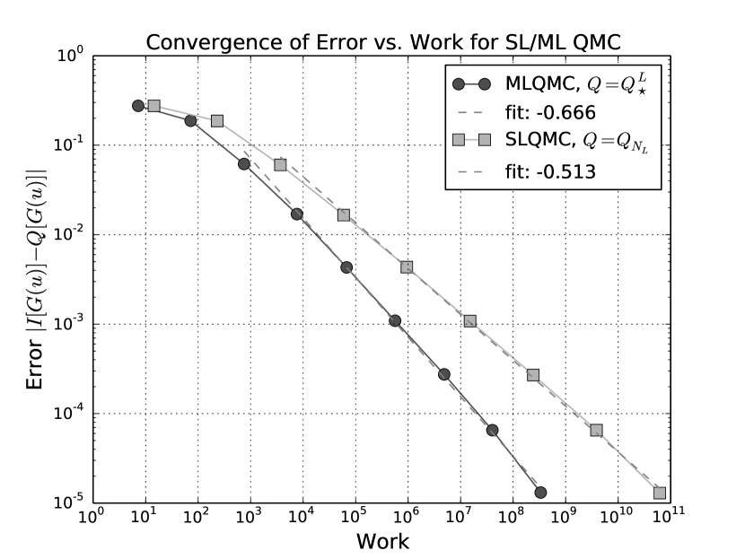
Fig. 1: Convergence of the error vs. the work. The theoretical rates are $-2/3$ for MLQMC and $-1/2$ for SLQMC. The slopes were computed by a linear fit using the last five measurements.

5 Conclusions

We designed and analyzed a multi-level QMC Petrov-Galerkin discretization for the approximate evaluation of functionals of solutions of countably affine parametric operator equations. The presently proposed algorithms extend on the one hand the single level higher order QMC algorithms proposed in [8], and on the other hand generalize the multi-level approach of [23] from first order finite elements and first order randomly-shifted lattice rules to higher order in both cases. At the same time, the class of admissible operator equations covered by our analysis is considerably larger, allowing in particular also indefinite, elliptic systems in non-smooth domains and space-time Galerkin discretizations of linear parabolic evolution problems. Numerical tests confirmed the theoretical results, and indicate that the presently obtained combined error bounds are attained in the practical range of discretization parameters, and that they can be used for practical algorithm design.

References

• [1] A. Barth, Ch. Schwab and N. Zollinger, Multi-level Monte Carlo finite element method for elliptic PDEs with stochastic coefficients. Numer. Math., 119 (2011), pp. 123–161.
• [2] J. Charrier, R. Scheichl and A. L. Teckentrup, Finite element error analysis of elliptic PDEs with random coefficients and its application to multilevel Monte Carlo methods. SIAM J. Numer. Anal., 51 (2013), pp. 322–352.
• [3] A. K. Cliffe, M. B. Giles, R. Scheichl and A. L. Teckentrup, Multilevel Monte Carlo methods and applications to elliptic PDEs with random coefficients. Comput. Vis. Sci., 14 (2011), pp. 3–15.
• [4] A. Cohen, R. DeVore and Ch. Schwab, Convergence rates of best $N$-term Galerkin approximation for a class of elliptic sPDEs, Found. Comput. Math., 10 (2010), pp. 615–646.
• [5] N. Collier, A.-L. Haji-Ali, F. Nobile, E. von Schwerin, R. Tempone, A Continuation Multilevel Monte Carlo algorithm, BIT, 55 (2015), pp. 399–432.
• [6] J. Dick, Walsh spaces containing smooth functions and Quasi-Monte Carlo rules of arbitrary high order, SIAM J. Numer. Anal., 46 (2008), pp. 1519–1553.
• [7] J. Dick, The decay of the Walsh coefficients of smooth functions, Bull. Aust. Math. Soc., 80 (2009), pp. 430–453.
• [8] J. Dick, F. Y. Kuo, Q. T. Le Gia, D. Nuyens and Ch. Schwab, Higher order QMC Galerkin discretization for parametric operator equations, SIAM J. Numer. Anal., 52 (2014), pp. 2676–2702.
• [9] J. Dick, F. Y. Kuo, and I. H. Sloan, High dimensional integration – the quasi-Monte Carlo way, Acta Numer. 22 (2013), pp. 133–288.
• [10] J. Dick and F. Pillichshammer, Digital Nets and Sequences. Discrepancy Theory and Quasi-Monte Carlo Integration, Cambridge University Press, Cambridge, 2010.
• [11] R.N. Gantner and Ch. Schwab, Computational Higher-Order QMC integration, Research Report 2014-24, Seminar for Applied Mathematics, ETH Zürich.
• [12] M. B. Giles, Multilevel Monte Carlo path simulation, Oper. Res., 56 (2008), pp. 607–617.
• [13] T. Goda, Good interlaced polynomial lattice rules for numerical integration in weighted Walsh spaces, J. Comput. Appl. Math., 285 (2015), pp. 279–294.
• [14] T. Goda and J. Dick, Construction of interlaced scrambled polynomial lattice rules of arbitrary high order, accepted for publication in Found. Comput. Math., DOI 10.1007/s10208-014-9226-8.
• [15] M. Hansen and Ch. Schwab, Analytic regularity and best $N$-term approximation of high dimensional parametric initial value problems, Vietnam Journal of Mathematics, 41 (2013), pp. 181–215.
• [16] H. Harbrecht, M. Peters and M. Siebenmorgen, On multilevel quadrature for elliptic stochastic partial differential equations, pp.161–179 in Sparse Grids and Applications, Lecture Notes in Computational Science and Engineering, Volume 88, 2013.
• [17] S. Heinrich, Monte Carlo complexity of global solution of integral equations, J. Complexity, 14 (1998), pp. 151–175.
• [18] V. H. Hoang and Ch. Schwab, Regularity and Generalized Polynomial Chaos Approximation of Parametric and Random Second-Order Hyperbolic Partial Differential Equations, Analysis and Applications (Singapore), 10 (2012), pp. 295–326.
• [19] V.H. Hoang and Ch. Schwab, Analytic regularity and polynomial approximation of stochastic, parametric elliptic multiscale PDEs, Analysis and Applications (Singapore), 11 (2013), 1350001, pp. 50.
• [20] A. Kunoth and Ch. Schwab, Analytic Regularity and GPC Approximation for Stochastic Control Problems Constrained by Linear Parametric Elliptic and Parabolic PDEs, SIAM J. Control and Optimization, 51 (2013), pp. 2442 – 2471.
• [21] F. Y. Kuo, Ch. Schwab and I. H. Sloan, Quasi-Monte Carlo finite element methods for a class of elliptic partial differential equations with random coefficient, SIAM J. Numer. Anal., 50 (2012), pp. 3351–3374.
• [22] F. Y. Kuo, Ch. Schwab and I. H. Sloan, Quasi-Monte Carlo methods for very high dimensional integration: the standard weighted-space setting and beyond, ANZIAM Journal, 53 (2011), pp. 1–37.
• [23] F. Y. Kuo, Ch. Schwab and I. H. Sloan, Multi-Level Quasi-Monte Carlo finite element methods for a class of elliptic partial differential equations with random coefficient, Found. Comput. Math., 15 (2015), pp. 411–449.
• [24] Y. Miyazaki, Spectral Asymptotics for Dirichlet Elliptic Operators with non-smooth Coefficients, Osaka Math. Journal, 46 (2009), pp. 441–460.
• [25] V. Nistor and C. Schwab, High order Galerkin approximations for parametric second order elliptic partial differential equations, Math. Mod. Meth. Appl. Sci., 23 (2013), pp. 1729–1760.
• [26] Cl. Schillings and Ch. Schwab, Sparse, Adaptive Smolyak Algorithms for Bayesian Inverse Problems, Inverse Problems, (2013), 065011.
• [27] Cl. Schillings and Ch. Schwab, Sparsity in Bayesian Inversion of Parametric Operator Equations, Inverse Problems, 30 (2014), 065007.
• [28] Ch. Schwab, QMC Galerkin discretizations of parametric operator equations, In: J. Dick, F. Y. Kuo, G. W. Peters and I. H. Sloan (eds.), Monte Carlo and Quasi-Monte Carlo Methods 2012, Springer Verlag, Heidelberg, 2013, pp. 613–629.
• [29] Ch. Schwab and C.J. Gittelson, Sparse tensor discretizations of high-dimensional parametric and stochastic PDEs, Acta Numerica, 20 (2011), pp. 291–467.
• [30] Ch. Schwab and R. A. Todor, Karhunen-Loève approximation of random fields by generalized fast multipole methods, J. Comput. Phy., 217 (2006), pp. 100–122.
• [31] M. A. Shubin, Pseudodifferential Operators and Spectral Theory, Springer Ser. Sov. Math., Springer Verlag, Berlin, 1987.
• [32] I. H. Sloan and H. Woźniakowski, When are Quasi-Monte Carlo algorithms efficient for high-dimensional integrals?, J. Complexity, 14 (1998), pp. 1–33.
• [33] A. L. Teckentrup, R. Scheichl, M. B. Giles, E. Ullmann, Further analysis of multilevel Monte Carlo methods for elliptic PDEs with random coefficients. Numer. Math., 125 (2013), pp. 569–600.
• [34] T. Yoshiki, Bounds on Walsh coefficients by dyadic difference and a new Koksma- Hlawka type inequality for Quasi-Monte Carlo integration. ArXiv:1504.03175 (2015).