Integral identities for an interfacial crack in an anisotropic bimaterial with an imperfect interface

Abstract

We study a crack lying along an imperfect interface in an anisotropic bimaterial. A method is devised where known weight functions for the perfect interface problem are used to obtain singular integral equations relating the tractions and displacements for both the in-plane and out-of-plane fields. The integral equations for the out-of-plane problem are solved numerically for orthotropic bimaterials with differing orientations of anisotropy and for different extents of interfacial imperfection. These results are then compared with finite element computations.

1 Introduction

Singular integral equations have played a significant role in the study of crack propagation in elastic media since their introduction by Muskhelishvili (1963) and have garnered much scientific attention (Sneddon, 1972). They have been used in the analysis of crack problems in complex domains containing an arbitrary number of wedges and layers separated by imperfect interfaces (Mishuris, 1997a, b); the resulting singular integral equations with fixed point singularities have been analysed by Duduchava (1979), based on the theory of linear singular operators (Gohberg and Krein, 1960). More recently, singular integral equations have been applied to problems involving interfacial cracks in both isotropic (Piccolroaz and Mishuris, 2013; Mishuris et al., 2014) and anisotropic bimaterials (Yu and Suo, 2000; Morini et al., 2013a). This paper extends the singular integral equation approach to an anisotropic bimaterial containing an imperfect interface.

Interfacial problems concerning a semi-infinite crack along a perfect interface in an anisotropic bimaterial have been considered in Suo (1990) through the use of the formalisms proposed by Stroh (1962) and Lekhnitskii (1963). Expressions were found for the stress intensity factors at the crack tip under the restriction of symmetric loading on the crack faces. Using weight function techniques introduced by Bueckner (1985) and developed further by Willis and Movchan (1995), an approach was developed to find stress intensity factors for an interfacial crack along a perfect interface under asymmetric loading for both the static and dynamic cases, see Morini et al. (2013b) and Pryce et al. (2013) respectively. More widely, weight functions are well developed in the literature for a wide range of fractured body geometries and allow for the evaluation of important constants that may act as fracture criteria. For instance, weight functions have been obtained for a corner crack in a plate of finite thickness (Zheng et al., 1996), a 3D semi-infinite crack in an infinite body (Kassir and Sih, 1973) and a crack lying perpendicular to the interface in a thin surface layer (Fett et al., 1996).

Imperfect interfaces provide a more physically realistic interpretation of a bimaterial than a perfect one, accounting for the fact that the interface between two materials is rarely sharp. Atkinson (1977) took this into account by suggesting the interface be replaced with a thin strip of finite thickness, which provided the bonding material occupying the strip is sufficiently soft may be replaced by so-called imperfect interface transmission conditions. These allow for an interfacial displacement jump in direct proportion to the traction, which is itself continuous across the interface (Antipov et al., 2001; Lenci, 2001; Mishuris, 2001). Such transmission conditions alter physical fields near the crack tip significantly; for instance the usual perfect interface square root stress singularity is no longer present and is instead replaced by a logarithmic singularity (Mishuris and Kuhn, 2001), although tractions remain bounded along the interface. More general imperfect interface transmission conditions were derived by Benveniste and Miloh (2001) which considered a thin curved isotropic layer of constant thickness, while Benveniste (2006) presented a general interface model for a 3D arbitrarily curved thin anisotropic interphase between two anisotropic solids.

Weight function techniques have been recently adapted to imperfect interface settings to quantify crack tip asymptotics in thin domains (Vellender et al., 2011), analyse problems of waves in thin waveguides (Vellender and Mishuris, 2012) and conduct perturbation analysis for large imperfectly bound bimaterials containing small defects (Vellender et al., 2013); the absence of the square root singularity means that the weight functions are not used to find stress intensity factors, but instead yield asymptotic constants which describe the crack tip opening displacement. This quantity was proposed for use in fracture criteria by Wells (1961) and Cottrell (1962) and later justified rigorously by Rice and Sorenson (1978), Shih et al. (1979) and Kanninen et al. (1979). Despite their great utility, the derivation of such weight functions is often not straightforward and so the approach deployed in the remainder of this paper efficiently utilises existing relationships between known weight functions without the need to derive further expressions.

The problem considered here is the anisotropic equivalent of that seen in Mishuris et al. (2014), which considered solely isotropic bimaterials. Besides this, perhaps the key novel feature in the present manuscript from a methodology viewpoint, is that known weight functions derived for the perfect interface problem are used in the derivation of singular integral equations for the soft imperfect interface case. This differs from previous approaches; for instance Mishuris et al. (2014) used specially-derived weight functions that took into account the local crack-tip behaviour brought about by the presence of imperfect interface transmission conditions, whereas the approach employed here uses existing perfect interface weight functions, which have fundamentally different behaviour near the crack tip to the physical solution in the imperfect interface problem.

The paper is structured as follows: Section 2 introduces the problem geometry and model for the imperfect interface. In Section 3, previously found results used in the derivation of the singular integral equations are discussed. These include the weight functions derived using the method of Willis and Movchan (1995) and the Betti formula which can be used to relate the weight functions to the physical fields along both the crack and imperfect interface. Section 4 concentrates on solving the out-of-plane (mode III) problem. Singular integral equations are derived and used to obtain the displacement jump across both the crack and interface for a number of orthotropic bimaterials with varying levels of interface imperfection. Finite element methods for the same physical problems are also used to obtain the same results and then a comparison is made between the results obtained from the two opposing methods. The in-plane problem is considered in Section 5, where singular integral equations are obtained for the mode I and mode II tractions and displacements and some computations are performed.

2 Problem formulation

We consider an infinite anisotropic bimaterial with an imperfect interface and a semi-infinite interfacial crack respectively lying along the positive and negative $x_{1}$ semi-axes. The materials above and below the $x_{1}$-axis will be denoted materials I and II respectively.

Figure 1: Geometry

The imperfect interface transmission conditions for $x_{1}>0$ are given by

$$\mathbf{t}(x_{1},0^{+})=\mathbf{t}(x_{1},0^{-}),$$ (1)

$$\mathbf{u}(x_{1},0^{+})-\mathbf{u}(x_{1},0^{-})=\mathbf{K}\mathbf{t}(x_{1},0^{+}),$$ (2)

where $\mathbf{t}=(t_{1},t_{2},t_{3})^{T}=(\sigma_{21},\sigma_{22},\sigma_{23})^{T}$ is the traction vector and $\mathbf{u}=(u_{1},u_{2},u_{3})^{T}$ is the displacement vector. The matrix $\mathbf{K}$ quantifies the extent of imperfection of the interface, with $\mathbf{K}=\mathbf{0}$ corresponding to the perfect interface. For an anisotropic bonding material, $\mathbf{K}$ has the following structure:

$$\mathbf{K}=\begin{pmatrix}K_{11}&K_{12}&0\\ K_{12}&K_{22}&0\\ 0&0&\kappa\end{pmatrix}.$$ (3)

The loading on the crack faces is considered known and given by

$$\mathbf{t}(x_{1},0^{+})=\mathbf{p}^{+}(x_{1}),\quad\mathbf{t}(x_{1},0^{-})=\mathbf{p}^{-}(x_{1}),\quad\text{for }x_{1}<0.$$ (4)

The geometry considered is illustrated in Figure 1. The only restriction imposed on $\mathbf{p}^{\pm}$ is that they must be self-balanced; note in particular that this allows for discontinuous and/or asymmetric loadings. The symmetric and skew-symmetric parts of the loading are given by $\langle\mathbf{p}\rangle$ and $\llbracket\mathbf{p}\rrbracket$ respectively, where the notation $\langle f\rangle$ and $\llbracket f\rrbracket$ respectively denote the average and jump of the argument function:

$$\langle f\rangle(x_{1})=\frac{1}{2}(f(x_{1},0^{+})+f(x_{1},0^{-})),\quad\llbracket f\rrbracket(x_{1})=f(x_{1},0^{+})-f(x_{1},0^{-}).$$

3 Application of existing weight functions

3.1 Weight functions

Bueckner (1985) defined weight functions as non-trivial singular solutions of the homogeneous traction-free problem. Willis and Movchan (1995) introduced weight functions in a mirrored domain and related physical quantities with the auxiliary weight functions via use of Betti’s identity; this procedure has been recently used to derive singular integral equations for isotropic bimaterials joined by an imperfect interface (Mishuris et al., 2014). The approach employed there required the use of weight functions that had been designed for an imperfect interface setting for isotropic bimaterials. In the spirit of the efficiency outlined in the introduction, we will in this section introduce a method where integral identities for the physical problem with an imperfect interface are found using existing weight functions formulated in a perfect interface setting. Such weight functions can be found in the paper of Morini et al. (2013b). Note that such weight functions play a role only as solutions to auxiliary problems and have no immediate physical interpretation; we refer the reader to Willis and Movchan (1995) for further details.

The weight function used is the solution of the problem with the crack occupying the positive $x_{1}$ axis with square-root singular displacement at the crack tip, as given in Morini et al. (2013b). The transmission conditions for the weight functions for $x_{1}<0$ are given as

$$\mathbf{\Sigma}(x_{1},0^{+})=\mathbf{\Sigma}(x_{1},0^{-}),$$ (5)

$$\mathbf{U}(x_{1},0^{+})=\mathbf{U}(x_{1},0^{-}),$$ (6)

where $\mathbf{U}$ is the singular displacement field and $\mathbf{\Sigma}$ is the corresponding traction field. Note in particular that condition (6) corresponds to a perfect interface weight function problem in contrast to the imperfect interface problem being physically considered.

It was shown in Morini et al. (2013b) that the following equations hold for the Fourier transforms of the symmetric and skew-symmetric parts of the weight function:

$$\llbracket\bar{\mathbf{U}}\rrbracket^{+}(\xi)=\frac{1}{|\xi|}(i\mathrm{sign}(\xi)\mathrm{Im}(\mathbf{H})-\mathrm{Re}(\mathbf{H}))\langle\bar{\mathbf{\Sigma}}\rangle^{-}(\xi);$$ (7)

$$\langle\bar{\mathbf{U}}\rangle(\xi)=\frac{1}{2|\xi|}(i\mathrm{sign}(\xi)\mathrm{Im}(\mathbf{W})-\mathrm{Re}(\mathbf{W}))\langle\bar{\mathbf{\Sigma}}\rangle^{-}(\xi),$$ (8)

where $\mathbf{H}=\mathbf{B}_{I}+\mathbf{B}^{\star}_{II}$ and $\mathbf{W}=\mathbf{B}_{I}-\mathbf{B}^{\star}_{II}$. Here, $\mathbf{B}_{I}$ and $\mathbf{B}_{II}$ are the surface admittance tensors of materials I and II respectively, superscript ^⋆ denotes complex conjugation and bars denote Fourier transforms with respect to $x_{1}$ defined as

$$\bar{f}(\xi)=\mathcal{F}[f](\xi)=\int\limits_{-\infty}^{\infty}f(x_{1})e^{i\xi x_{1}}\mathrm{d}x_{1}.$$ (9)

The matrices $\mathbf{H}$ and $\mathbf{W}$ have the form

$$\mathbf{H}=\begin{pmatrix}H_{11}&-i\beta\sqrt{H_{11}H_{22}}&0\\ i\beta\sqrt{H_{11}H_{22}}&H_{22}&0\\ 0&0&H_{33}\end{pmatrix},\quad\mathbf{W}=\begin{pmatrix}\delta_{1}H_{11}&i\gamma\sqrt{H_{11}H_{22}}&0\\ -i\gamma\sqrt{H_{11}H_{22}}&\delta_{2}H_{22}&0\\ 0&0&\delta_{3}H_{33}\end{pmatrix}.$$ (10)

The entries of these matrices can be expressed in terms of the components of the material compliance tensors, $\mathbf{S}$. Explicit expressions for $\mathbf{H}$ and $\mathbf{W}$ for orthotropic bimaterials are given in the appendix.

3.2 Betti formula

In this section, the Betti formula is extended to the case of general asymmetrical loading applied at the crack surfaces. The Betti formula is used in order to relate the physical solution to the weight function, which is a special singular solution to the homogeneous problem with traction-free crack faces (Willis and Movchan, 1995; Piccolroaz et al., 2007).

Applying the Betti formula to a semi-circular domain in the half-plane $x_{2}>0$, whose straight boundary is the line $x_{2}=0^{+}$, and whose radius $R\to\infty$, the following equation is obtained

$$\int\limits_{(x_{2}=0^{+})}\Big{\{}\boldsymbol{\mathcal{R}}\mathbf{U}(x_{1}^{\prime}-x_{1},0^{+})\cdot\mathbf{t}(x_{1},0^{+})-\boldsymbol{\mathcal{R}}\mathbf{\Sigma}(x_{1}^{\prime}-x_{1},0^{+})\cdot\mathbf{u}(x_{1},0^{+})\Big{\}}\mathrm{d}x_{1}=0.$$ (11)

where $\boldsymbol{\mathcal{R}}$ is a rotation matrix given by

$$\begin{pmatrix}-1&0&0\\ 0&1&0\\ 0&0&-1\end{pmatrix}.$$

Another equation can be derived by applying the Betti formula to a semi-circular domain in the half-plane $x_{2}<0$ and taking the limit, $R\to\infty$, which after some manipulation in the spirit of Piccolroaz et al. (2009) for example, yields

$$\boldsymbol{\mathcal{R}}\llbracket\mathbf{U}\rrbracket*\langle\mathbf{t}\rangle^{(+)}-\boldsymbol{\mathcal{R}}\langle\mathbf{\Sigma}\rangle^{(-)}*\llbracket\mathbf{u}\rrbracket=-\boldsymbol{\mathcal{R}}\llbracket\mathbf{U}\rrbracket*\langle\mathbf{p}\rangle-\boldsymbol{\mathcal{R}}\langle\mathbf{U}\rangle*\llbracket\mathbf{p}\rrbracket,$$ (12)

where the convolutions are taken with respect to $x_{1}$, that is

$$(f*g)(x_{1})=\int_{-\infty}^{\infty}f(x_{1}-t)g(t)\mathrm{d}t,$$

and superscripts ^(±) denote the restriction of the preceding function to the respective semi-$x_{1}$-axis. Applying Fourier transforms then gives

$$\bar{\llbracket\mathbf{U}\rrbracket}^{T}\boldsymbol{\mathcal{R}}\bar{\langle\mathbf{t}\rangle}^{+}-(\bar{\langle\mathbf{\Sigma}\rangle}^{-})^{T}\boldsymbol{\mathcal{R}}\bar{\llbracket\mathbf{u}\rrbracket}=-\bar{\llbracket\mathbf{U}\rrbracket}^{T}\boldsymbol{\mathcal{R}}\bar{\langle\mathbf{p}\rangle}-\bar{\langle\mathbf{U}\rangle}^{T}\boldsymbol{\mathcal{R}}\bar{\llbracket\mathbf{p}\rrbracket}.$$ (13)

Note that the exact nature of the weight functions $\mathbf{U}$ and $\mathbf{\Sigma}$ used in this analysis have not been specified at this stage and so identity (13) is valid for a large class of weight functions. In particular, this allows for the use of perfect interface weight functions for the imperfect interface physical setting. In the case of perfect interface physical solution and weight functions, the corresponding analysis has been done in Piccolroaz and Mishuris (2013); Morini et al. (2013b), for isotropic and anisotropic materials respectively, while for imperfect interfaces joining isotropic bodies, details can be found in Mishuris et al. (2014).

4 Integral identities for mode III

4.1 Derivation of integral identities

We now seek boundary integral equations relating the mode III interfacial traction and displacement jump over the crack in the anisotropic bimaterial. This will utilise the Betti identity in order to relate the physical solution with the perfect interface weight functions.

Considering only the mode III components of (13) the following equation holds:

$$\bar{\llbracket U\rrbracket}(\xi)\overline{\langle t\rangle^{(+)}}(\xi)-\overline{\langle\Sigma\rangle^{(-)}}(\xi)\bar{\llbracket u\rrbracket}(\xi)=-\bar{\llbracket U\rrbracket}(\xi)\bar{\langle p\rangle}(\xi)-\bar{\langle U\rangle}(\xi)\bar{\llbracket p\rrbracket}(\xi),$$ (14)

where the subscripts have been removed for notational brevity. Splitting $\llbracket U\rrbracket$ into the sum of $\llbracket U\rrbracket^{(\pm)}$ and also separating $\llbracket u\rrbracket$ into the sum of $\llbracket u\rrbracket^{(\pm)}$ gives

$$\overline{\llbracket U\rrbracket^{(+)}}(\xi)\overline{\langle t\rangle^{(+)}}(\xi)+\overline{\llbracket U\rrbracket^{(-)}}(\xi)\overline{\langle t\rangle^{(+)}}(\xi)-\overline{\langle\Sigma\rangle^{(-)}}(\xi)\overline{\llbracket u\rrbracket^{(+)}}(\xi)-\overline{\langle\Sigma\rangle^{(-)}}(\xi)\overline{\llbracket u\rrbracket^{(+)}}(\xi)=$$

$$-\bar{\llbracket U\rrbracket}(\xi)\bar{\langle p\rangle}(\xi)-\bar{\langle U\rangle}(\xi)\bar{\llbracket p\rrbracket}(\xi).$$ (15)

Note that if imperfect interface weight functions are used, then the second and third terms of the left hand side of (15) immediately due to the transmission conditions (Vellender et al., 2013). However, using perfect interface weight functions, this is not true.

Using the transmission conditions, $\overline{\llbracket U\rrbracket^{(-)}}=0$ and $\overline{\llbracket u\rrbracket^{(+)}}=\kappa\bar{\langle t\rangle}$ yields

$$\overline{\langle t\rangle^{(+)}}-\left(\frac{\overline{\langle\Sigma\rangle^{(-)}}}{\overline{\llbracket U\rrbracket^{(+)}}-\kappa\overline{\langle\Sigma\rangle^{(-)}}}\right)\overline{\llbracket u\rrbracket^{(-)}}=-\left(\frac{\bar{\llbracket U\rrbracket}}{\overline{\llbracket U\rrbracket^{(+)}}-\kappa\overline{\langle\Sigma\rangle^{(-)}}}\right)\bar{\langle p\rangle}-\left(\frac{\bar{\langle U\rangle}}{\overline{\llbracket U\rrbracket^{(+)}}-\kappa\overline{\langle\Sigma\rangle^{(-)}}}\right)\bar{\llbracket p\rrbracket}.$$ (16)

From equations (7) and (8) the following relationships hold for the mode III components of the weight functions:

$$\bar{\llbracket U\rrbracket}=\overline{\llbracket U\rrbracket^{(+)}}(\xi)=-\frac{H_{33}}{|\xi|}\overline{\langle\Sigma\rangle^{(-)}}(\xi);\quad\langle\bar{U}\rangle=-\frac{\delta_{3}H_{33}}{2|\xi|}\overline{\langle\Sigma\rangle^{(-)}}(\xi)=\frac{\delta_{3}}{2}\llbracket\bar{U}\rrbracket(\xi);$$ (17)

when combined with equation (16) the following relationship is obtained:

$$\overline{\langle t\rangle^{(+)}}-A(\xi)\overline{\llbracket u\rrbracket^{(-)}}=-(1+\kappa A(\xi))\bar{\langle p\rangle}-\frac{\delta_{3}}{2}(1+\kappa A(\xi))\bar{\llbracket p\rrbracket},$$ (18)

where

$$A(\xi)=-\frac{|\xi|}{\kappa|\xi|+\kappa\mathcal{H}_{33}},\qquad\mathcal{H}_{33}=\frac{H_{33}}{\kappa}.$$

Applying the inverse Fourier transform to equation (18) for the two cases, $x_{1}<0$ and $x_{1}>0$, the following relationships are obtained:

$$\mathcal{F}^{-1}_{x_{1}<0}\left[A(\xi)\overline{\llbracket u\rrbracket^{(-)}}\right]=\mathcal{F}^{-1}_{x_{1}<0}\left[(1+\kappa A(\xi))\bar{\langle p\rangle}\right]+\frac{\delta_{3}}{2}\mathcal{F}^{-1}_{x_{1}<0}\left[(1+\kappa A(\xi))\bar{\llbracket p\rrbracket}\right];$$ (19)

$$\langle t\rangle^{(+)}(x_{1})=\mathcal{F}^{-1}_{x_{1}>0}\left[A(\xi)\overline{\llbracket u\rrbracket^{(-)}}\right]-\mathcal{F}^{-1}_{x_{1}>0}\left[(1+\kappa A(\xi))\bar{\langle p\rangle}\right]-\frac{\delta_{3}}{2}\mathcal{F}^{-1}_{x_{1}>0}\left[(1+\kappa A(\xi))\bar{\llbracket p\rrbracket}\right].$$ (20)

To calculate these inversions the following relationships are used:

$$\mathcal{F}^{-1}\left[A(\xi)\bar{f}(\xi)\right]=\frac{1}{\pi\kappa}\left(S_{\mathcal{H}_{33}}\ast f^{\prime}\right)(x_{1});$$ (21)

$$\mathcal{F}^{-1}\left[(1+\kappa A(\xi))\bar{f}(\xi)\right]=-\frac{\mathcal{H}_{33}}{\pi}\left(T_{\mathcal{H}_{33}}\ast f\right)(x_{1}),$$ (22)

where

$$S_{\mathcal{H}_{33}}(x_{1})=\mathrm{sign}(x_{1})\mathrm{si}(\mathcal{H}_{33}|x_{1}|)\cos(\mathcal{H}_{33}|x_{1}|)-\mathrm{sign}(x_{1})\mathrm{ci}(\mathcal{H}_{33}|x_{1}|)\sin(\mathcal{H}_{33}|x_{1}|),$$ (23)

$$T_{\mathcal{H}_{33}}(x_{1})=\mathrm{si}(\mathcal{H}_{33}|x_{1}|)\sin(\mathcal{H}_{33}|x_{1}|)-\mathrm{ci}(\mathcal{H}_{33}|x_{1}|)\cos(\mathcal{H}_{33}|x_{1}|),$$ (24)

and si and ci are the sine and cosine integral functions respectively, given by

$$\mathrm{si}(x_{1})=-\int_{x_{1}}^{\infty}\frac{\sin t}{t}\mathrm{d}t,\quad\mathrm{ci}(x_{1})=-\int_{x_{1}}^{\infty}\frac{\cos t}{t}\mathrm{d}t.$$ (25)

These functions have the same properties as their counterparts from the isotropic case considered by Mishuris et al. (2014), but with different constants. In particular, the function $S_{\mathcal{H}_{33}}(x_{1})$ behaves as

$$S_{\mathcal{H}_{33}}(x_{1})=-\frac{\pi}{2}\mathrm{sign}(x_{1})+O(|x_{1}|),\>x_{1}\to 0,\qquad S_{\mathcal{H}_{33}}(x_{1})=-\frac{\mathrm{sign}(x_{1})}{\mathcal{H}_{33}|x_{1}|}+O\left(\frac{1}{|x_{1}|^{3}}\right),\>x_{1}\to\pm\infty,$$ (26)

while $T_{\mathcal{H}_{33}}(x_{1})$ has behaviour of the form

$$T_{\mathcal{H}_{33}}(x_{1})=\ln(\mathcal{H}_{33}|x_{1}|)+O(1),\>x_{1}\to 0,\qquad T_{\mathcal{H}_{33}}(x_{1})=-\frac{1}{\mathcal{H}_{33}^{2}|x_{1}|^{2}}+O\left(\frac{1}{|x_{1}|^{3}}\right),\>x_{1}\to\pm\infty.$$ (27)

We introduce convolution operators $\mathcal{S}_{\mathcal{H}_{33}}$ and $\mathcal{T}_{\mathcal{H}_{33}}$, as well as projection operators $\mathcal{P}_{\pm}$:

$$\mathcal{S}_{\mathcal{H}_{33}}\varphi(x_{1})=(S_{\mathcal{H}_{33}}\ast\varphi)(x_{1}),\qquad\mathcal{T}_{\mathcal{H}_{33}}\varphi(x_{1})=(T_{\mathcal{H}_{33}}\ast\varphi)(x_{1}),$$ (28)

$$\mathcal{P}_{\pm}\varphi(x_{1})=\begin{cases}\varphi(x_{1})\quad\pm x_{1}\geq 0,\\ 0\quad\mathrm{otherwise},\end{cases}$$ (29)

in order to rewrite the identities (19) and (20) as

$$\frac{1}{\pi\kappa}\mathcal{S}_{\mathcal{H}_{33}}^{(s)}\frac{\partial\llbracket u\rrbracket^{(-)}}{\partial x_{1}}-\frac{1}{\pi\kappa}\llbracket u\rrbracket^{(-)}(0^{-})S_{\mathcal{H}_{33}}(x_{1})=-\frac{\mathcal{H}_{33}}{\pi}\mathcal{T}_{\mathcal{H}_{33}}^{(s)}\langle p\rangle(x_{1})-\frac{\delta_{3}\mathcal{H}_{33}}{2\pi}\mathcal{T}_{\mathcal{H}_{33}}^{(s)}\llbracket p\rrbracket(x_{1}),\quad x_{1}<0,$$ (30)

$$\langle t\rangle^{(+)}(x_{1})=\frac{1}{\pi\kappa}\mathcal{S}_{\mathcal{H}_{33}}^{(c)}\frac{\partial\llbracket u\rrbracket^{(-)}}{\partial x_{1}}-\frac{1}{\pi\kappa}\llbracket u\rrbracket^{(-)}(0^{-})S_{\mathcal{H}_{33}}(x_{1}) +\frac{\mathcal{H}_{33}}{\pi}\mathcal{T}_{\mathcal{H}_{33}}^{(c)}\langle p\rangle(x_{1})$$

$$+\frac{\delta_{3}\mathcal{H}_{33}}{2\pi}\mathcal{T}_{\mathcal{H}_{33}}^{(c)}\llbracket p\rrbracket(x_{1}),\quad x_{1}>0,$$ (31)

where

$$\mathcal{S}_{\mathcal{H}_{33}}^{(s)}=\mathcal{P}_{-}\mathcal{S}_{\mathcal{H}_{33}}\mathcal{P}_{-},\qquad\mathcal{T}_{\mathcal{H}_{33}}^{(s)}=\mathcal{P}_{-}\mathcal{T}_{\mathcal{H}_{33}}\mathcal{P}_{-},$$ (32)

are singular operators and

$$\mathcal{S}_{\mathcal{H}_{33}}^{(c)}=\mathcal{P}_{+}\mathcal{S}_{\mathcal{H}_{33}}\mathcal{P}_{-},\qquad\mathcal{T}_{\mathcal{H}_{33}}^{(c)}=\mathcal{P}_{+}\mathcal{T}_{\mathcal{H}_{33}}\mathcal{P}_{-},$$ (33)

are compact. The second term on the left hand side of (30) and right hand side of (4.1) appear as a result of the discontinuity of the derivative of $\llbracket u\rrbracket^{(-)}$ at $x_{1}=0$.

4.2 Alternative integral identities

The integral identities (30) and (4.1) can be formulated in alternative ways, which depending upon the specific problem parameters and loadings, can aid the ease with which computations may be performed. Combining equations (21), (22) and (28) yields the auxiliary relationship

$$-\frac{\mathcal{H}_{33}}{\pi}\mathcal{T}_{\mathcal{H}_{33}}\varphi=\mathcal{I}\varphi+\frac{1}{\pi}\mathcal{S}_{\mathcal{H}_{33}}\varphi^{\prime}.$$ (34)

Using this relationship, equations (30) and (4.1) can be rewritten as follows:

$$-\frac{\mathcal{H}_{33}}{\pi\kappa}\mathcal{T}_{\mathcal{H}_{33}}^{(s)}\llbracket u\rrbracket^{(-)}-\frac{1}{\kappa}\llbracket u\rrbracket^{(-)}= \frac{1}{\pi}\mathcal{S}_{\mathcal{H}_{33}}^{(s)}\frac{\partial\langle p\rangle}{\partial x_{1}}-\frac{1}{\pi}\langle p\rangle(0^{-})S_{\mathcal{H}_{33}}+\langle p\rangle$$

$$+\frac{\delta_{3}}{2\pi}\mathcal{S}_{\mathcal{H}_{33}}^{(s)}\frac{\partial\llbracket p\rrbracket}{\partial x_{1}}-\frac{\delta_{3}}{2\pi}\llbracket p\rrbracket(0^{-})S_{\mathcal{H}_{33}}+\frac{\delta_{3}}{2}\llbracket p\rrbracket,\quad x_{1}<0;$$ (35)

$$\langle t\rangle^{(+)}=-\frac{\mathcal{H}_{33}}{\pi\kappa}\mathcal{T}_{\mathcal{H}_{33}}^{(c)}\llbracket u\rrbracket^{(-)}-\frac{1}{\pi}\mathcal{S}_{\mathcal{H}_{33}}^{(c)}\frac{\partial\langle p\rangle}{\partial x_{1}}+ \frac{1}{\pi}\langle p\rangle(0^{-})S_{\mathcal{H}_{33}}+\langle p\rangle$$

$$-\frac{\delta_{3}}{2\pi}\mathcal{S}_{\mathcal{H}_{33}}^{(c)}\frac{\partial\llbracket p\rrbracket}{\partial x_{1}}+\frac{\delta_{3}}{2\pi}\llbracket p\rrbracket(0^{-})S_{\mathcal{H}_{33}},\quad x_{1}>0.$$ (36)

It is also possible to write these equations using only the operator $\mathcal{T}_{\mathcal{H}_{33}}$:

$$-\frac{\mathcal{H}_{33}}{\pi\kappa}\mathcal{T}_{\mathcal{H}_{33}}^{(s)}\llbracket u\rrbracket^{(-)}-\frac{1}{\kappa}\llbracket u\rrbracket^{(-)}=-\frac{\mathcal{H}_{33}}{\pi}\mathcal{T}_{\mathcal{H}_{33}}^{(s)}\langle p\rangle-\frac{\delta_{3}\mathcal{H}_{33}}{2\pi}\mathcal{T}_{\mathcal{H}_{33}}^{(s)}\llbracket p\rrbracket,\quad x_{1}<0;$$ (37)

$$\langle t\rangle^{(+)}=-\frac{\mathcal{H}_{33}}{\pi\kappa}\mathcal{T}_{\mathcal{H}_{33}}^{(c)}\llbracket u\rrbracket^{(-)}+\frac{\mathcal{H}_{33}}{\pi}\mathcal{T}_{\mathcal{H}_{33}}^{(c)}\langle p\rangle+\frac{\delta_{3}\mathcal{H}_{33}}{2\pi}\mathcal{T}_{\mathcal{H}_{33}}^{(c)}\llbracket p\rrbracket,\quad x_{1}>0,$$ (38)

or solely the operator $\mathcal{S}_{\mathcal{H}_{33}}$:

$$\frac{1}{\pi\kappa} \mathcal{S}_{\mathcal{H}_{33}}^{(s)}\frac{\partial\llbracket u\rrbracket^{(-)}}{\partial x_{1}}-\frac{1}{\pi\kappa}\llbracket u\rrbracket^{(-)}(0^{-})S_{\mathcal{H}_{33}}=$$

$$\frac{1}{\pi}\mathcal{S}_{\mathcal{H}_{33}}^{(s)}\frac{\partial\langle p\rangle}{\partial x_{1}}-\frac{1}{\pi}\langle p\rangle(0^{-})S_{\mathcal{H}_{33}}+\langle p\rangle+\frac{\delta_{3}}{2\pi}\mathcal{S}_{\mathcal{H}_{33}}^{(s)}\frac{\partial\llbracket p\rrbracket}{\partial x_{1}}-\frac{\delta_{3}}{2\pi}\llbracket p\rrbracket(0^{-})S_{\mathcal{H}_{33}}+\frac{\delta_{3}}{2}\llbracket p\rrbracket,\quad x_{1}<0;$$ (39)

$$\langle t\rangle^{(+)}=\frac{1}{\pi\kappa} \mathcal{S}_{\mathcal{H}_{33}}^{(c)}\frac{\partial\llbracket u\rrbracket^{(-)}}{\partial x_{1}}-\frac{1}{\pi\kappa}\llbracket u\rrbracket^{(-)}(0^{-})S_{\mathcal{H}_{33}}$$

$$- \frac{1}{\pi}\mathcal{S}_{\mathcal{H}_{33}}^{(c)}\frac{\partial\langle p\rangle}{\partial x_{1}}+\frac{1}{\pi}\langle p\rangle(0^{-})S_{\mathcal{H}_{33}}+\langle p\rangle-\frac{\delta_{3}}{2\pi}\mathcal{S}_{\mathcal{H}_{33}}^{(c)}\frac{\partial\llbracket p\rrbracket}{\partial x_{1}}+\frac{\delta_{3}}{2\pi}\llbracket p\rrbracket(0^{-})S_{\mathcal{H}_{33}},\quad x_{1}>0.$$ (40)

Each of the four formulations have advantages for numerical computations depending on the mechanical parameters of the problem and which quantities are known or unknown. The merits of alternative formulations for the analogous isotropic case have been discussed in detail in Mishuris et al. (2014) and we refer the reader to that paper for further discussion.

4.3 Numerical results

4.3.1 Results from singular integral equations

In this section, the integral identities found previously will be used to calculate the jump in displacement over the crack and imperfect interface between two orthotropic materials. Results for finite element simulations using COMSOL will also be presented and compared to the results using the integral identity approach derived in the previous subsection.

We will present results for the displacement jump $\llbracket u\rrbracket$. Note for the Mode III case that for $x_{1}>0$, the interfacial tractions and displacement jump $\llbracket u\rrbracket$ are straightforwardly related via the imperfect interface transmission conditions (2). In particular for the Mode III displacement jump, the relationship is as follows:

$$\llbracket u\rrbracket(x_{1})=\kappa\langle t\rangle(x_{1}),\qquad x_{1}>0.$$ (41)

Here, we only consider tractions along the crack/interface line; discussions of full radial asymptotics (for stress and displacement) and their relationship to the displacement jump can be found in Lenci (2001); Mishuris (2001); Antipov et al. (2001); Vellender et al. (2013), among others.

For orthotropic materials, the material parameters $H_{33}$ and $\delta_{3}$ are given in terms of the components of the material compliance tensor, $\mathbf{S}$, in the appendix. It is possible to express $S_{44}$ and $S_{55}$ in terms of the shear moduli, $\mu_{ij}$ of the material:

$$S_{44}=\frac{1}{\mu_{23}},\qquad S_{55}=\frac{1}{\mu_{13}}.$$ (42)

In our computations, the same orthotropic material will be used as material I and II. However, the axes corresponding to each axis of symmetry of the material in the lower half-plane is altered. The parameters used for the computations presented are shown in Table 1. The values of $\mu_{12}$ are given in Table 1 to illustrate that the materials considered are the same but differently oriented. Henceforth, the material above the crack (I) will be material A from Table 1.

Orientation	$\mu_{23}$	$\mu_{13}$	$\mu_{12}$
A	1	2/3	1/2
B	1	1/2	2/3
C	1/2	2/3	1

Table 1: Material properties

We first consider a symmetric distribution of loadings given by

$$\llbracket p\rrbracket(x_{1})=0,\qquad\langle p\rangle(x_{1})=-\frac{F}{l}e^{\frac{x_{1}}{l}}.$$ (43)

Figure 2 plots the normalised displacement jump along the $x_{1}$-axis induced by the above loading for the three possible orientations for material II for two different degrees of interface imperfection which have been computed by numerically solving the integral equations (37) and (38) using an iterative scheme in Mathematica. The normalised displacement jump is denoted $\llbracket u^{\ast}\rrbracket$ and defined by

$$\llbracket u^{*}\rrbracket=\frac{1}{F\left[\sqrt{S_{44}S_{55}}\right]_{I}}\llbracket u\rrbracket.$$ (44)

A normalised traction, $t^{*}$, is also used in the calculations and is related to the normalised displacement jump by the relationship $\llbracket u^{*}\rrbracket=\kappa^{*}t^{*}$, where

$$t^{*}=\frac{l}{F}t,\qquad\kappa^{*}=\frac{1}{l\left[\sqrt{S_{44}S_{55}}\right]_{I}}\kappa.$$ (45)

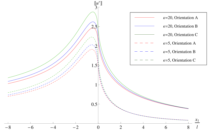
Figure 2: Graph of normalised displacement jump over the crack and interface induced by loading (43).

Figure 2 shows that a higher value of $\kappa$ gives a higher jump in displacement across the crack and interface for all orientations of the material II; this result is expected as a larger $\kappa$ refers to a less stiff interface. It is also seen that for the same value of $\kappa$, the orientation of the anisotropy has a diminishing effect along the interface ($x_{1}>0$) as the distance from the crack tip is increased.

The difference in orientation of material II has a clear effect on the jumps in displacement shown in Figure 2, with the same behaviour observed for both values of $\kappa$ studied here. The highest jump in both cases is seen for orientation C in the lower half-plane. This is due to the lower shear moduli contributing to the mode-III fields in this case. Orientation A leads to the smallest displacement jump; this is due to the higher shear moduli in the out-of-plane direction.

In order to demonstrate that the method is applicable for asymmetric as well as symmetric loadings, we present in Figure 3 a similar plot, but instead using asymmetric loadings of the form

$$p^{+}(x_{1})=-\frac{F}{l}e^{x_{1}/l},\qquad p^{-}(x_{1})=\frac{F}{l^{2}}x_{1}e^{x_{1}/l}.$$ (46)

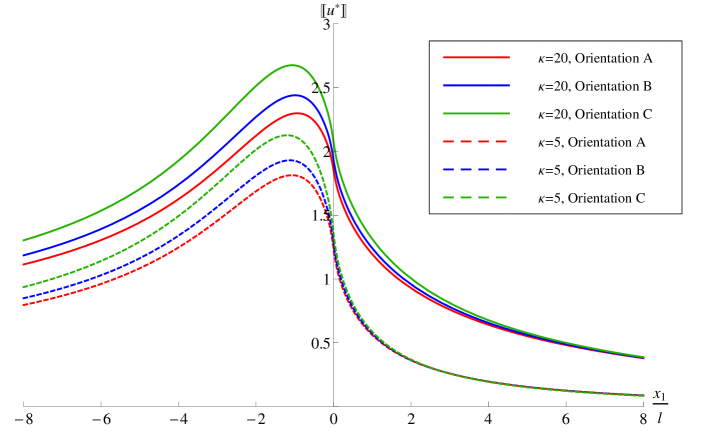
Figure 3: Displacement jump for asymmetric loading.

4.3.2 Finite element results

We now compare results from finite element simulations performed in COMSOL for a crack along an imperfect interface with computations from the integral equations. When using COMSOL it is not possible to implement the transmission conditions (1) and (2) across the interface. Instead, a very thin layer of a softer material is used for the interface and the properties of that material are varied to obtain the desired value for $\kappa$ (see for instance Antipov et al. (2001)). Also, it is not possible to realise an infinite geometry in COMSOL and therefore a very large, finite geometry is used as an approximation. These issues with the finite element model demonstrate the advantage of the boundary integral formulation, since the issues of the very fine meshing required in the interface layer and the large geometries of the main material bodies are respectively replaced by imperfect interface transmission conditions and the lower dimensional nature of the boundary problem. We present results comparing the two approaches in a case where the soft interface layer is not too thin in order to demonstrate the comparability of the two approaches.

An example colour map of the Mode-III displacement from COMSOL is shown in Figure 4, using material orientation A for both main material bodies and an interface layer corresponding to $\kappa=20$.

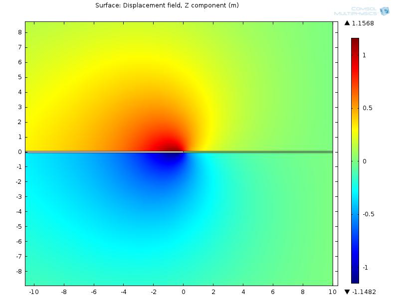
Figure 4: Finite element computations of displacement jump, using a thin densely-meshed soft layer in place of the imperfect interface.

Using COMSOL, values for the displacement jump over the crack and interface have been extracted for a number of points near the crack tip for two of the examples shown in Figure 2. The results of these comparisons are shown in Figure 5 and Table 2.

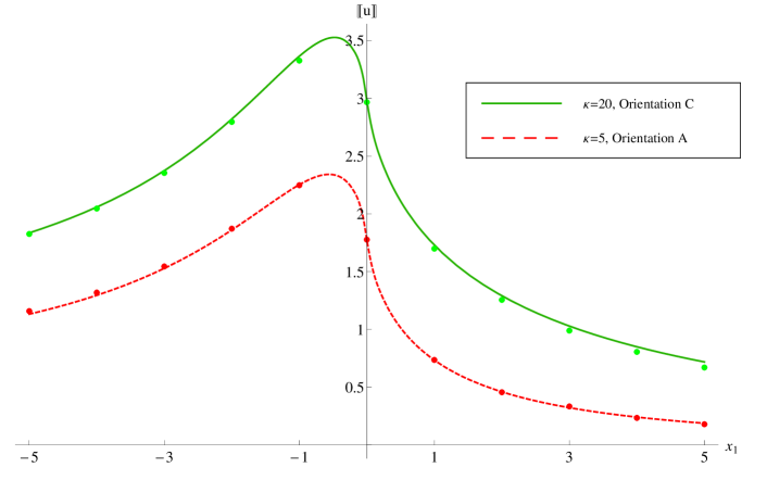
Figure 5: Graph of the comparison between displacement jumps from Mathematica and COMSOL. The lines show the results of computations from the integral equations while finite element computations are represented by dots.

Material	-5	-4	-3	-2	-1	0	1	2	3	4	5
A, $\kappa=5$	2.30	1.81	1.07	0.61	0.20	0.06	0.18	0.70	3.41	2.77	4.66
C, $\kappa=20$	0.53	0.62	0.84	0.87	1.13	0.55	1.80	2.75	3.81	5.19	6.70

Table 2: Percentage difference between Mathematica and COMSOL.

Figure 5 shows good agreement between the results from the singular integral equations and those obtained from finite element methods. The difference in results is smallest at the crack tip but more error can be seen at a further distance along both the crack and interface, which is emphasised by the larger percentage errors shown in Table 2. This is likely caused by the finite geometry that was used in COMSOL which leads to an influence caused by the outer boundaries.

5 Integral identities for mode I and II

5.1 Derivation of integral identities

Heretofore, we have derived integral identities for the mode III regime only. This section seeks to find boundary integral equations relating the mode I and II interfacial traction and displacement jump over the crack in an imperfectly bound anisotropic bimaterial. For the mode I and II components the following equation holds

$$\bar{\llbracket\mathbf{U}\rrbracket}^{T}\boldsymbol{\mathcal{R}}\overline{\langle\mathbf{t}\rangle^{(+)}}-\overline{\langle\mathbf{\Sigma}\rangle^{(-)}}^{T}\boldsymbol{\mathcal{R}}\bar{\llbracket\mathbf{u}\rrbracket}=-\bar{\llbracket\mathbf{U}\rrbracket}^{T}\boldsymbol{\mathcal{R}}\bar{\langle\mathbf{p}\rangle}-\bar{\langle\mathbf{U}\rangle}^{T}\boldsymbol{\mathcal{R}}\bar{\llbracket\mathbf{p}\rrbracket}.$$ (47)

The matrices and vectors shown here contain only the mode I and II components from (13). The $2\times 2$ matrices $\bar{\mathbf{U}}$ and $\bar{\mathbf{\Sigma}}$ consist of two linearly independent weight functions (Piccolroaz et al., 2009).

Splitting $\bar{\llbracket\mathbf{U}\rrbracket}$ into the sum of $\overline{\llbracket\mathbf{U}\rrbracket^{(\pm)}}$ and $\bar{\llbracket\mathbf{u}\rrbracket}$ into $\overline{\llbracket\mathbf{u}\rrbracket^{(\pm)}}$, where (as previously) superscripts ^(±) denote the restriction of the preceding function to the respective semi-$x_{1}$-axis, gives

$$\overline{\llbracket\mathbf{U}\rrbracket^{(+)}}^{T}\boldsymbol{\mathcal{R}}\overline{\langle\mathbf{t}\rangle^{(+)}}+\overline{\llbracket\mathbf{U}\rrbracket^{(-)}}^{T}\boldsymbol{\mathcal{R}}\overline{\langle\mathbf{t}\rangle^{(+)}}-\overline{\langle\mathbf{\Sigma}\rangle^{(-)}}^{T}\boldsymbol{\mathcal{R}}\overline{\llbracket\mathbf{u}\rrbracket^{(+)}} -\overline{\langle\mathbf{\Sigma}\rangle^{(-)}}^{T}\boldsymbol{\mathcal{R}}\overline{\llbracket\mathbf{u}\rrbracket^{(-)}}$$

$$=-\bar{\llbracket\mathbf{U}\rrbracket}^{T}\boldsymbol{\mathcal{R}}\bar{\langle\mathbf{p}\rangle}-\bar{\langle\mathbf{U}\rangle}^{T}\boldsymbol{\mathcal{R}}\bar{\llbracket\mathbf{p}\rrbracket}.$$ (48)

Applying the boundary conditions, $\overline{\llbracket\mathbf{U}\rrbracket^{(-)}}=0$ and $\overline{\llbracket\mathbf{u}\rrbracket^{(+)}}=\mathbf{K}\overline{\langle\mathbf{t}\rangle^{(+)}}$, along with equations (7) and (8) gives the following expression:

$$\overline{\langle\mathbf{t}\rangle^{(+)}}-\mathbf{B}(\xi)\frac{\xi}{i}\overline{\llbracket\mathbf{u}\rrbracket^{(-)}}=-\mathbf{C}(\xi)\bar{\langle\mathbf{p}\rangle}-\mathbf{A}(\xi)\bar{\llbracket\mathbf{p}\rrbracket},$$ (49)

where

$$\mathbf{A}(\xi)=\frac{1}{2}\boldsymbol{\mathcal{R}}^{-1}(|\xi|\mathbf{K}^{*}+\mathbf{R_{H}}-i\mathrm{sign}(\xi)\mathbf{I_{H}})^{-T}(\mathbf{R_{W}}-i\mathrm{sign}(\xi)\mathbf{I_{W}})^{T}\boldsymbol{\mathcal{R}},$$

$$\mathbf{B}(\xi)=-i\boldsymbol{\mathcal{R}}^{-1}(\xi\mathbf{K}^{*}+\mathrm{sign}(\xi)\mathbf{R_{H}}-i\mathbf{I_{H}})^{-T}\boldsymbol{\mathcal{R}},$$

$$\mathbf{C}(\xi)=\boldsymbol{\mathcal{R}}^{-1}(|\xi|\mathbf{K}^{*}+\mathbf{R_{H}}-i\mathrm{sign}(\xi)\mathbf{I_{H}})^{-T}(\mathbf{R_{H}}-i\mathrm{sign}(\xi)\mathbf{I_{H}})^{T}\boldsymbol{\mathcal{R}}.$$

Here, $\mathbf{R_{H}}=\mathrm{Re}(\mathbf{H})$, $\mathbf{R_{W}}=\mathrm{Re}(\mathbf{W})$, $\mathbf{I_{H}}=\mathrm{Im}(\mathbf{H})$, $\mathbf{I_{W}}=\mathrm{Im}(\mathbf{W})$ and $\mathbf{K}^{*}=\boldsymbol{\mathcal{R}}\mathbf{K}\boldsymbol{\mathcal{R}}$. Full expressions for matrices $\mathbf{A}(\xi),\mathbf{B}(\xi)$ and $\mathbf{C}(\xi)$ can be found in the appendix.

Applying the inverse Fourier transform to equation (49) for the two cases, $x_{1}<0$ and $x_{1}>0$, the following relationships are obtained:

$$\mathcal{F}^{-1}_{x_{1}<0}\left[\mathbf{B}(\xi)\frac{\xi}{i}\overline{\llbracket\mathbf{u}\rrbracket^{(-)}}\right]=\mathcal{F}^{-1}_{x_{1}<0}\left[\mathbf{C}(\xi)\bar{\langle\mathbf{p}\rangle}\right]+\mathcal{F}^{-1}_{x_{1}<0}\left[\mathbf{A}(\xi)\bar{\llbracket\mathbf{p}\rrbracket}\right];$$ (50)

$$\langle\mathbf{t}\rangle(x_{1})=\mathcal{F}^{-1}_{x_{1}>0}\left[\mathbf{B}(\xi)\frac{\xi}{i}\overline{\llbracket\mathbf{u}\rrbracket^{(-)}}\right]-\mathcal{F}^{-1}_{x_{1}>0}\left[\mathbf{C}(\xi)\bar{\langle\mathbf{p}\rangle}\right]-\mathcal{F}^{-1}_{x_{1}>0}\left[\mathbf{A}(\xi)\bar{\llbracket\mathbf{p}\rrbracket}\right].$$ (51)

The inverse Fourier transforms of the matrices $\mathbf{A}(\xi)$, $\mathbf{B}(\xi)$ and $\mathbf{C}(\xi)$ are derived in the appendix of this paper. The singular integral equations obtained for the in-plane fields are thus

$$\boldsymbol{\mathcal{B}}^{(s)}\frac{\partial\llbracket\mathbf{u}\rrbracket^{(-)}}{\partial x_{1}}+\frac{1}{\pi d_{2}(\xi_{2}-\xi_{1})}\sum_{j=1}^{2}\mathbf{B}_{R}^{(j)}T_{\xi_{j}}(x_{1}) \llbracket\mathbf{u}\rrbracket^{(-)}(0^{-})+\frac{1}{\pi d_{2}(\xi_{2}-\xi_{1})}\sum_{j=1}^{2}\mathbf{B}_{I}^{(j)}S_{\xi_{j}}(x_{1})\llbracket\mathbf{u}\rrbracket^{(-)}(0^{-})$$

$$=\boldsymbol{\mathcal{C}}^{(s)}\langle\mathbf{p}\rangle(x_{1})+\boldsymbol{\mathcal{A}}^{(s)}\llbracket\mathbf{p}\rrbracket(x_{1}),\quad\text{for }x_{1}<0,$$ (52)

$$\langle\mathbf{t}\rangle(x_{1})= \boldsymbol{\mathcal{B}}^{(c)}\frac{\partial\llbracket\mathbf{u}\rrbracket^{(-)}}{\partial x_{1}}+\frac{1}{\pi d_{2}(\xi_{2}-\xi_{1})}\sum_{j=1}^{2}\mathbf{B}_{R}^{(j)}T_{\xi_{j}}(x_{1})\llbracket\mathbf{u}\rrbracket^{(-)}(0^{-})$$

$$+\frac{1}{\pi d_{2}(\xi_{2}-\xi_{1})}\sum_{j=1}^{2}\mathbf{B}_{I}^{(j)}S_{\xi_{j}}(x_{1})\llbracket\mathbf{u}\rrbracket^{(-)}(0^{-})-\boldsymbol{\mathcal{C}}^{(c)}\langle\mathbf{p}\rangle(x_{1})-\boldsymbol{\mathcal{A}}^{(c)}\llbracket\mathbf{p}\rrbracket(x_{1}),\quad\text{for }x_{1}>0.$$ (53)

The operators used in equations (52) and (53) are given by

$$\boldsymbol{\mathcal{A}}^{(s,c)}=-\frac{1}{2\pi d_{2}(\xi_{2}-\xi_{1})}\left\{\sum_{j=1}^{2}\mathbf{A}_{R}^{(j)}\mathcal{T}^{(s,c)}_{\xi_{j}}(x_{1})+\sum_{j=1}^{2}\mathbf{A}_{I}^{(j)}\mathcal{S}^{(s,c)}_{\xi_{j}}(x_{1})\right\},$$ (54)

$$\boldsymbol{\mathcal{B}}^{(s,c)}=-\frac{1}{\pi d_{2}(\xi_{2}-\xi_{1})}\left\{\sum_{j=1}^{2}\mathbf{B}_{R}^{(j)}\mathcal{T}^{(s,c)}_{\xi_{j}}(x_{1})+\sum_{j=1}^{2}\mathbf{B}_{I}^{(j)}\mathcal{S}^{(s,c)}_{\xi_{j}}(x_{1})\right\},$$ (55)

$$\boldsymbol{\mathcal{C}}^{(s,c)}=-\frac{1}{\pi d_{2}(\xi_{2}-\xi_{1})}\left\{\sum_{j=1}^{2}\mathbf{C}_{R}^{(j)}\mathcal{T}^{(s,c)}_{\xi_{j}}(x_{1})+\sum_{j=1}^{2}\mathbf{C}_{I}^{(j)}\mathcal{S}^{(s,c)}_{\xi_{j}}(x_{1})\right\}.$$ (56)

5.2 Numerical examples

In this section we present an illustrative example of applying the derived integral equations (52) and (53) to find the in-plane tractions and displacement jump when an asymmetrical, mode I loading is applied to the crack faces. For the purpose of these calculations, incompressible orthotropic materials will be used. It was shown by Itskov and Aksel (2002) that for such materials only four parameters are required to express the components of $\mathbf{S}$, which are related to the matrices $\mathbf{H}$ and $\mathbf{W}$ (as seen in Appendix A). The components are

$$S_{11}=\frac{1}{E_{1}},\quad S_{22}=\frac{1}{E_{2}},\quad S_{66}=\frac{1}{\mu_{12}},$$

$$S_{12}=\frac{1}{2}\left(\frac{1}{E_{3}}-\frac{1}{E_{1}}-\frac{1}{E_{2}}\right),$$ (57)

where $E_{i}$ are the Young’s moduli of the material in question. The materials considered here will have the properties shown in Table 3.

Material	$E_{1}$	$E_{2}$	$E_{3}$	$\mu_{12}$
I	20	10	10	5
II	20	10	15	5

Table 3: Material parameters.

We present computations resulting from an applied asymmetric crack face loading of the form

$$\mathbf{p}^{+}(x_{1})=\begin{pmatrix}0\\ -\frac{F}{l}e^{x_{1}/l}\end{pmatrix},\quad\mathbf{p}^{-}(x_{1})=\begin{pmatrix}0\\ \frac{F}{l^{2}}x_{1}e^{x_{1}/l}\end{pmatrix},$$ (58)

with $F=1$ and $l=1$; the interfacial imperfection parameters are $K_{11}=10$, $K_{12}=2$, $K_{22}=3$. The interfacial tractions are shown in Figure 6, along with the displacement jump in the $x_{1}$ and $x_{2}$ directions. Note that since the crack face loadings were applied in the $x_{2}$-direction, the displacement jump across the crack and interface, as well as the interfacial traction, is dominant in that direction. Note in particular that the presence of the imperfect interface causes components of stress to remain bounded at the crack tip along the interface/crack line, in contrast to the analogous perfect interface problem.

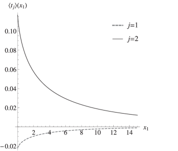
Figure 6: In-plane displacement jump across the crack and interface line (left), and interfacial stresses for $x_{1}>0$ (right).

6 Conclusions

Singular integral equations have been derived which relate the loading on crack faces to the consequent crack opening displacement and interfacial tractions for a semi-infinite crack situated along a soft anisotropic imperfect interface for an anisotropic bimaterial. The derivation made efficient use of perfect interface weight functions applied to an imperfect interface physical problem; this did not require derivation of new weight functions. As in the previously studied analogous isotropic problem, the imperfect interface’s presence causes a logarithmic singularity in the kernel of the integral operator. Alternative formulations have been presented for the mode III case and used to perform computations for orthotropic materials, which display a good degree of accuracy when compared against finite element simulations.

References

Appendix A Bimaterial matrices $\mathbf{H}$ and $\mathbf{W}$ for orthotropic bimaterials

The matrices $\mathbf{H}$ and $\mathbf{W}$ have the form

$$\mathbf{H}=\begin{pmatrix}H_{11}&-i\beta\sqrt{H_{11}H_{22}}&0\\ i\beta\sqrt{H_{11}H_{22}}&H_{22}&0\\ 0&0&H_{33}\end{pmatrix},\quad\mathbf{W}=\begin{pmatrix}\delta_{1}H_{11}&i\gamma\sqrt{H_{11}H_{22}}&0\\ -i\gamma\sqrt{H_{11}H_{22}}&\delta_{2}H_{22}&0\\ 0&0&\delta_{3}H_{33}\end{pmatrix}.$$ (59)

For orthotropic materials it is possible to obtain explicit expressions for the these matrices in terms of the components of the material compliance tensors.

The out-of-plane components are given by

$$H_{33}=\left[\sqrt{S_{44}S_{55}}\right]_{I}+\left[\sqrt{S_{44}S_{55}}\right]_{II},\quad\delta_{3}=\frac{\left[\sqrt{S_{44}S_{55}}\right]_{I}-\left[\sqrt{S_{44}S_{55}}\right]_{II}}{H_{33}}.$$ (60)

The in-plane components of $\mathbf{H}$ can be found in Morini et al. (2013b) and are given as

$$H_{11}=\left[2n\lambda^{1/4}\sqrt{S_{11}S_{22}}\right]_{I}+\left[2n\lambda^{1/4}\sqrt{S_{11}S_{22}}\right]_{II},$$ (61)

$$H_{22}=\left[2n\lambda^{-1/4}\sqrt{S_{11}S_{22}}\right]_{I}+\left[2n\lambda^{-1/4}\sqrt{S_{11}S_{22}}\right]_{II},$$ (62)

$$\beta=\frac{\left[S_{12}+\sqrt{S_{11}S_{22}}\right]_{II}-\left[S_{12}+\sqrt{S_{11}S_{22}}\right]_{I}}{\sqrt{H_{11}H_{22}}},$$ (63)

where

$$\lambda=\frac{S_{11}}{S_{22}},\quad n=\sqrt{(1+\rho)/2},\quad\rho=\frac{2S_{12}+S_{66}}{2\sqrt{S_{11}S_{22}}}.$$

The in-plane components of $\mathbf{W}$ were also given in Morini et al. (2013b):

$$\delta_{1}=\frac{\left[2n\lambda^{1/4}\sqrt{S_{11}S_{22}}\right]_{I}-\left[2n\lambda^{1/4}\sqrt{S_{11}S_{22}}\right]_{II}}{H_{11}},$$ (64)

$$\delta_{2}=\frac{\left[2n\lambda^{-1/4}\sqrt{S_{11}S_{22}}\right]_{I}-\left[2n\lambda^{-1/4}\sqrt{S_{11}S_{22}}\right]_{II}}{H_{22}},$$ (65)

$$\gamma=\frac{\left[S_{12}+\sqrt{S_{11}S_{22}}\right]_{I}+\left[S_{12}+\sqrt{S_{11}S_{22}}\right]_{II}}{\sqrt{H_{11}H_{22}}}.$$ (66)

Appendix B The matrices $\mathbf{A}(\xi)$, $\mathbf{B}(\xi)$ and $\mathbf{C}(\xi)$

Matrices $\mathbf{A}(\xi)$, $\mathbf{B}(\xi)$ and $\mathbf{C}(\xi)$ have the following form

$$\mathbf{A}(\xi)=\frac{1}{2D}\begin{pmatrix}A_{11}&A_{12}\\ A_{21}&A_{22}\end{pmatrix},\quad\mathbf{B}(\xi)=\frac{1}{D}\begin{pmatrix}B_{11}&B_{12}\\ B_{21}&B_{22}\end{pmatrix},\quad\mathbf{C}(\xi)=\frac{1}{D}\begin{pmatrix}C_{11}&C_{12}\\ C_{21}&C_{22}\end{pmatrix}$$ (67)

where the denominator $D$ is defined as

$$D=d_{0}+d_{1}|\xi|+d_{2}|\xi|^{2},$$ (68)

$$d_{0}=H_{11}H_{22}(1-\beta^{2}),\quad d_{1}=K_{11}H_{22}+K_{22}H_{11},\quad d_{2}=K_{11}K_{22}-K_{12}^{2},$$

and the elements $A_{ij}$, $B_{ij}$, $C_{ij}$ are given by

$$A_{11}=H_{11}H_{22}(\delta_{1}+\beta\gamma)+|\xi|(\delta_{1}H_{11}K_{22}-i\gamma K_{12}\sqrt{H_{11}H_{22}}\text{ sign}(\xi)),$$

$$A_{12}=-i\text{ sign}(\xi)H_{22}\sqrt{H_{11}H_{22}}(\gamma+\beta\delta_{2})-|\xi|(i\gamma K_{22}\sqrt{H_{11}H_{22}}\text{ sign}(\xi)+\delta_{2}H_{22}K_{12}),$$

$$A_{21}=i\text{ sign}(\xi)H_{11}\sqrt{H_{11}H_{22}}(\delta_{1}\beta+\gamma)-|\xi|(\delta_{1}H_{11}K_{12}-i\gamma K_{11}\sqrt{H_{11}H_{22}}\text{ sign}(\xi)),$$

$$A_{22}=H_{11}H_{22}(\beta\gamma+\delta_{2})+|\xi|(\delta_{2}H_{22}K_{11}+i\gamma K_{12}\sqrt{H_{11}H_{22}}\text{ sign}(\xi)),$$

$$B_{11}=-i(\xi K_{22}+H_{22}\text{ sign}(\xi)),$$

$$B_{12}=i\xi K_{12}-\beta\sqrt{H_{11}H_{22}},$$

$$B_{21}=i\xi K_{12}+\beta\sqrt{H_{11}H_{22}},$$

$$B_{22}=-i(\xi K_{11}+H_{11}\text{ sign}(\xi)),$$

$$C_{11}=H_{11}H_{22}(1-\beta^{2})+|\xi|(H_{11}K_{22}+i\beta K_{12}\sqrt{H_{11}H_{22}}\text{ sign}(\xi)),$$

$$C_{12}=-|\xi|(H_{22}K_{12}-i\beta\text{ sign}(\xi)K_{22}\sqrt{H_{11}H_{22}}),$$

$$C_{21}=-|\xi|(H_{11}K_{12}+i\beta\text{ sign}(\xi)K_{11}\sqrt{H_{11}H_{22}}),$$

$$C_{22}=H_{11}H_{22}(1-\beta^{2})+|\xi|(H_{22}K_{11}-i\beta K_{12}\sqrt{H_{11}H_{22}}\text{ sign}(\xi)).$$

Appendix C Inverse Fourier transforms of matrices $\mathbf{A}(\xi)$, $\mathbf{B}(\xi)$ and $\mathbf{C}(\xi)$

C.1 General procedure

The method outlined in Mishuris et al. (2014) is used in order to perform the Fourier inversion of the matrices $\mathbf{A}(\xi)$, $\mathbf{B}(\xi)$ and $\mathbf{C}(\xi)$. The denominator $D$ defined in (68) is factorised in the following manner

$$D=d_{2}(|\xi|+\xi_{1})(|\xi|+\xi_{2}),$$ (69)

where

$$\xi_{1,2}=\frac{d_{1}\mp\sqrt{d_{1}^{2}-4d_{2}d_{0}}}{2d_{2}}>0,$$ (70)

The typical term to invert is of the form

$$F(\xi)=\frac{F_{R}+F_{R}^{\dagger}|\xi|}{D}+i\frac{F_{I}\text{ sign}(\xi)+F_{I}^{\dagger}\xi}{D},$$ (71)

The function $F$ has the following property

$$F(-\xi)=\overline{F(\xi)},$$ (72)

therefore, the Fourier inversion can be obtained as

$$\mathcal{F}^{-1}[F(\xi)]=\frac{1}{\pi}\mathrm{Re}\int_{0}^{\infty}F(\xi)e^{-ix_{1}\xi}\mathrm{d}\xi=\frac{1}{\pi}\int_{0}^{\infty}\mathrm{Re}[F(\xi)]\cos(x_{1}\xi)\mathrm{d}\xi+\frac{1}{\pi}\int_{0}^{\infty}\mathrm{Im}[F(\xi)]\sin(x_{1}\xi)\mathrm{d}\xi,$$ (73)

where for $\xi>0$

$$\mathrm{Re}[F(\xi)]=\frac{F_{R}+F_{R}^{\dagger}\xi}{D}=\sum_{j=1}^{2}\frac{F_{R}^{(j)}}{d_{2}(\xi_{2}-\xi_{1})(\xi+\xi_{j})},$$ (74)

$$\mathrm{Im}[F(\xi)]=\frac{F_{I}+F_{I}^{\dagger}\xi}{D}=\sum_{j=1}^{2}\frac{F_{I}^{(j)}}{d_{2}(\xi_{2}-\xi_{1})(\xi+\xi_{j})},$$ (75)

and

$$F_{R,I}^{(1)}=F_{R,I}-F_{R,I}^{\dagger}\xi_{1},\quad F_{R,I}^{(2)}=-F_{R,I}+F_{R,I}^{\dagger}\xi_{2}.$$ (76)

The following formulae can now be used

$$\int_{0}^{\infty}\mathrm{Re}[F(\xi)]\cos(x_{1}\xi)\mathrm{d}\xi=\sum_{j=1}^{2}\frac{F_{R}^{(j)}}{d_{2}(\xi_{2}-\xi_{1})}\int_{0}^{\infty}\frac{\cos(x_{1}\xi)}{\xi+\xi_{j}}\mathrm{d}\xi=-\frac{1}{d_{2}(\xi_{2}-\xi_{1})}\sum_{j=1}^{2}F_{R}^{(j)}T_{\xi_{j}}(x_{1}),$$ (77)

$$\int_{0}^{\infty}\mathrm{Im}[F(\xi)]\sin(x_{1}\xi)\mathrm{d}\xi=\sum_{j=1}^{2}\frac{F_{I}^{(j)}}{d_{2}(\xi_{2}-\xi_{1})}\int_{0}^{\infty}\frac{\sin(x_{1}\xi)}{\xi+\xi_{j}}\mathrm{d}\xi=-\frac{1}{d_{2}(\xi_{2}-\xi_{1})}\sum_{j=1}^{2}F_{I}^{(j)}S_{\xi_{j}}(x),$$ (78)

where functions $S_{\xi_{j}}(x)$ and $T_{\xi_{j}}(x)$ are defined as in (23) and (24), respectively.

Finally the Fourier inversion of the general term $F(\xi)$ as given as

$$\mathcal{F}^{-1}[F(\xi)]=-\frac{1}{\pi d_{2}(\xi_{2}-\xi_{1})}\left\{\sum_{j=1}^{2}F_{R}^{(j)}T_{\xi_{j}}(x_{1})+\sum_{j=1}^{2}F_{I}^{(j)}S_{\xi_{j}}(x_{1})\right\}.$$ (79)

C.2 Fourier inversion of $\mathbf{A}(\xi)$.

For $\xi>0$, $\mathbf{A}(\xi)$ can be written as

$$\mathbf{A}(\xi)=\frac{1}{2D}(\mathbf{A}_{R}+\mathbf{A}_{R}^{\dagger}\xi)+\frac{i}{2D}(\mathbf{A}_{I}+\mathbf{A}_{I}^{\dagger}\xi)=\frac{1}{2d_{2}(\xi_{2}-\xi_{1})}\left\{\sum_{j=1}^{2}\frac{1}{\xi+\xi_{j}}\mathbf{A}_{R}^{(j)}+i\sum_{j=1}^{2}\frac{1}{\xi+\xi_{j}}\mathbf{A}_{I}^{(j)}\right\},$$ (80)

where

$$\mathbf{A}_{R}=H_{11}H_{22}\begin{pmatrix}\delta_{1}+\beta\gamma&0\\ 0&\delta_{2}+\beta\gamma\end{pmatrix},\quad\mathbf{A}_{R}^{\dagger}=\begin{pmatrix}\delta_{1}H_{11}K_{22}&-\delta_{2}H_{22}K_{12}\\ -\delta_{1}H_{11}K_{12}&\delta_{2}H_{22}K_{11}\end{pmatrix},$$ (81)

$$\mathbf{A}_{I}=\sqrt{H_{11}H_{22}}\begin{pmatrix}0&-H_{22}(\delta_{2}\beta+\gamma)\\ H_{11}(\delta_{1}\beta+\gamma)&0\end{pmatrix},\quad\mathbf{A}_{I}^{\dagger}=\gamma\sqrt{H_{11}H_{22}}\begin{pmatrix}-K_{12}&-K_{22}\\ K_{11}&K_{12}\end{pmatrix},$$ (82)

$$\mathbf{A}_{R}^{(1)}=\mathbf{A}_{R}-\mathbf{A}_{R}^{\dagger}\xi_{1}=\begin{pmatrix}H_{11}(H_{22}(\delta_{1}+\beta\gamma)-\delta_{1}K_{22}\xi_{1})&\delta_{2}H_{22}K_{12}\xi_{1}\\ \delta_{1}H_{11}K_{12}\xi_{1}&H_{22}(H_{11}(\delta_{2}+\beta\gamma)-\delta_{2}K_{11}\xi_{1})\end{pmatrix},$$ (83)

$$\mathbf{A}_{R}^{(2)}=-\mathbf{A}_{R}+\mathbf{A}_{R}^{\dagger}\xi_{2}=\begin{pmatrix}-H_{11}(H_{22}(\delta_{1}+\beta\gamma)-\delta_{1}K_{22}\xi_{2})&-\delta_{2}H_{22}K_{12}\xi_{2}\\ -\delta_{1}H_{11}K_{12}\xi_{2}&-H_{22}(H_{11}(\delta_{2}+\beta\gamma)-\delta_{2}K_{11}\xi_{2})\end{pmatrix},$$ (84)

$$\mathbf{A}_{I}^{(1)}=\mathbf{A}_{I}-\mathbf{A}_{I}^{\dagger}\xi_{1}=\sqrt{H_{11}H_{22}}\begin{pmatrix}\gamma K_{12}\xi_{1}&-H_{22}(\beta\delta_{2}+\gamma)+\gamma K_{22}\xi_{1}\\ H_{11}(\beta\delta_{1}+\gamma)-\gamma K_{11}\xi_{1}&-\gamma K_{12}\xi_{1}\end{pmatrix},$$ (85)

$$\mathbf{A}_{I}^{(2)}=-\mathbf{A}_{I}+\mathbf{A}_{I}^{\dagger}\xi_{2}=\sqrt{H_{11}H_{22}}\begin{pmatrix}-\gamma K_{12}\xi_{2}&H_{22}(\beta\delta_{2}+\gamma)-\gamma K_{22}\xi_{2}\\ -H_{11}(\beta\delta_{1}+\gamma)+\gamma K_{11}\xi_{2}&\gamma K_{12}\xi_{2}\end{pmatrix}.$$ (86)

The Fourier inverse of the matrix $\mathbf{A}(\xi)$ is given by

$$\mathcal{F}^{-1}[\mathbf{A}(\xi)]=-\frac{1}{2\pi d_{2}(\xi_{2}-\xi_{1})}\left\{\sum_{j=1}^{2}\mathbf{A}_{R}^{(j)}T_{\xi_{j}}(x_{1})+\sum_{j=1}^{2}\mathbf{A}_{I}^{(j)}S_{\xi_{j}}(x_{1})\right\}.$$ (87)

C.3 Fourier inversion of the matrix $\mathbf{B}(\xi)$.

For $\xi>0$ $\mathbf{B}(\xi)$ can be written as

$$\mathbf{B}(\xi)=\frac{1}{D}(\mathbf{B}_{R}+\mathbf{B}_{R}^{\dagger}\xi)+\frac{i}{D}(\mathbf{B}_{I}+\mathbf{B}_{I}^{\dagger}\xi)=\frac{1}{d_{2}(\xi_{2}-\xi_{1})}\left\{\sum_{j=1}^{2}\frac{1}{\xi+\xi_{j}}\mathbf{B}_{R}^{(j)}+i\sum_{j=1}^{2}\frac{1}{\xi+\xi_{j}}\mathbf{B}_{I}^{(j)}\right\},$$ (88)

where

$$\mathbf{B}_{R}=\beta\sqrt{H_{11}H_{22}}\begin{pmatrix}0&-1\\ 1&0\end{pmatrix},\quad\mathbf{B}_{R}^{\dagger}=\mathbf{0},$$ (89)

$$\mathbf{B}_{I}=\begin{pmatrix}-H_{22}&0\\ 0&-H_{11}\end{pmatrix},\quad\mathbf{B}_{I}^{\dagger}=\begin{pmatrix}-K_{22}&K_{12}\\ K_{12}&-K_{11}\end{pmatrix},$$ (90)

$$\mathbf{B}_{R}^{(1)}=\mathbf{B}_{R}-\mathbf{B}_{R}^{\dagger}\xi_{1}=\beta\sqrt{H_{11}H_{22}}\begin{pmatrix}0&-1\\ 1&0\end{pmatrix},$$ (91)

$$\mathbf{B}_{R}^{(2)}=-\mathbf{B}_{R}+\mathbf{B}_{R}^{\dagger}\xi_{2}=\beta\sqrt{H_{11}H_{22}}\begin{pmatrix}0&1\\ -1&0\end{pmatrix},$$ (92)

$$\mathbf{B}_{I}^{(1)}=\mathbf{B}_{I}-\mathbf{B}_{I}^{\dagger}\xi_{1}=\begin{pmatrix}-H_{22}+K_{22}\xi_{1}&-K_{12}\xi_{1}\\ -K_{12}\xi_{1}&-H_{11}+K_{11}\xi_{1}\end{pmatrix},$$ (93)

$$\mathbf{B}_{I}^{(2)}=-\mathbf{B}_{I}+\mathbf{B}_{I}^{\dagger}\xi_{2}=\begin{pmatrix}H_{22}-K_{22}\xi_{2}&K_{12}\xi_{2}\\ K_{12}\xi_{2}&H_{11}-K_{11}\xi_{2}\end{pmatrix}.$$ (94)

The Fourier inverse of the matrix $\mathbf{B}(\xi)$ is then

$$\mathcal{F}^{-1}[\mathbf{B}(\xi)]=-\frac{1}{\pi d_{2}(\xi_{2}-\xi_{1})}\left\{\sum_{j=1}^{2}\mathbf{B}_{R}^{(j)}T_{\xi_{j}}(x_{1})+\sum_{j=1}^{2}\mathbf{B}_{I}^{(j)}S_{\xi_{j}}(x_{1})\right\}.$$ (95)

C.4 Fourier inversion of the matrix $\mathbf{C}(\xi)$.

For $\xi>0$ $\mathbf{C}(\xi)$ can be written as

$$\mathbf{C}(\xi)=\frac{1}{D}(\mathbf{C}_{R}+\mathbf{C}_{R}^{\dagger}\xi)+\frac{i}{D}(\mathbf{C}_{I}+\mathbf{C}_{I}^{\dagger}\xi)=\frac{1}{d_{2}(\xi_{2}-\xi_{1})}\left\{\sum_{j=1}^{2}\frac{1}{\xi+\xi_{j}}\mathbf{C}_{R}^{(j)}+i\sum_{j=1}^{2}\frac{1}{\xi+\xi_{j}}\mathbf{C}_{I}^{(j)}\right\},$$ (96)

where

$$\mathbf{C}_{R}=\begin{pmatrix}H_{11}H_{22}(1-\beta^{2})&0\\ 0&H_{11}H_{22}(1-\beta^{2})\end{pmatrix},\quad\mathbf{C}_{R}^{\dagger}=\begin{pmatrix}H_{11}K_{22}&-H_{22}K_{12}\\ -H_{11}K_{12}&H_{22}K_{11}\end{pmatrix},$$ (97)

$$\mathbf{C}_{I}=\mathbf{0},\quad\mathbf{C}_{I}^{\dagger}=\beta\sqrt{H_{11}H_{22}}\begin{pmatrix}K_{12}&K_{22}\\ -K_{11}&-K_{12}\end{pmatrix},$$ (98)

$$\mathbf{C}_{R}^{(1)}=\mathbf{C}_{R}-\mathbf{C}_{R}^{\dagger}\xi_{1}=\begin{pmatrix}H_{11}(H_{22}(1-\beta^{2})-K_{22}\xi_{1})&H_{22}K_{12}\xi_{1}\\ H_{11}K_{12}\xi_{1}&H_{22}(H_{11}(1-\beta^{2})-K_{11}\xi_{1})\end{pmatrix},$$ (99)

$$\mathbf{C}_{R}^{(2)}=-\mathbf{C}_{R}+\mathbf{C}_{R}^{\dagger}\xi_{2}=\begin{pmatrix}-H_{11}(H_{22}(1-\beta^{2})-K_{22}\xi_{2})&-H_{22}K_{12}\xi_{2}\\ -H_{11}K_{12}\xi_{2}&-H_{22}(H_{11}(1-\beta^{2})-K_{11}\xi_{2})\end{pmatrix},$$ (100)

$$\mathbf{C}_{I}^{(1)}=\mathbf{C}_{I}-\mathbf{C}_{I}^{\dagger}\xi_{1}=\beta\sqrt{H_{11}H_{22}}\xi_{1}\begin{pmatrix}-K_{12}&-K_{22}\\ K_{11}&K_{12}\end{pmatrix},$$ (101)

$$\mathbf{C}_{I}^{(2)}=-\mathbf{C}_{I}+\mathbf{C}_{I}^{\dagger}\xi_{2}=-\beta\sqrt{H_{11}H_{22}}\xi_{2}\begin{pmatrix}-K_{12}&-K_{22}\\ K_{11}&K_{12}\end{pmatrix}.$$ (102)

The Fourier inverse of the matrix $\mathbf{C}(\xi)$ is then

$$\mathcal{F}^{-1}[\mathbf{C}(\xi)]=-\frac{1}{\pi d_{2}(\xi_{2}-\xi_{1})}\left\{\sum_{j=1}^{2}\mathbf{C}_{R}^{(j)}T_{\xi_{j}}(x_{1})+\sum_{j=1}^{2}\mathbf{C}_{I}^{(j)}S_{\xi_{j}}(x_{1})\right\}.$$ (103)

References

• Antipov et al. (2001) Antipov, Y. A., Avila-Pozos, O., Kolaczkowski, S. T., Movchan, A. B., 2001. Mathematical model of delamination cracks on imperfect interfaces. Int. J. Solids Struct. 38(36-37), 6665–6697.
• Atkinson (1977) Atkinson, C., 1977. On stress singularities and interfaces in linear elastic fracture mechanics. Int. J. Fracture 13, 807–820.
• Benveniste (2006) Benveniste, Y., 2006. A general interface model for a three-dimensional curved thin anisotropic interphase between two anisotropic media. J. Mech. Phys. Solids 54(4), 708–734.
• Benveniste and Miloh (2001) Benveniste, Y., Miloh, T., 2001. Imperfect soft and stiff interfaces in two-dimensional elasticity. Mech. Materials 33, 309–323.
• Bueckner (1985) Bueckner, H. F., 1985. Weight functions and fundamental fields for the penny-shaped and the half plane crack in three-space. Int. J. Solids Struct. 23, 57–93.
• Cottrell (1962) Cottrell, A. H., 1962. Theoretical aspects of radiation damage and brittle fracture in steel pressure vessels. Iron Steel Institute Special Report 69, 281–296.
• Duduchava (1979) Duduchava, R., 1979. Integral equations with fixed singularities. Teubner, Leipzig.
• Fett et al. (1996) Fett, T., Diegele, E., Munz, D., Rizzi, G., 1996. Weight functions for edge cracks in thin surface layers. Int. J. Fract. 81 (3), 205–215.
• Gohberg and Krein (1960) Gohberg, I. C., Krein, M. G., 1960. Systems of integral equations on a half line with kernels depending on the difference of arguments (english translation). Amer. Math. Soc. Transl. 14, 217–287.
• Itskov and Aksel (2002) Itskov, M., Aksel, N., 2002. Elastic constants and their admissible values for incompressible and slightly compressible anisotropic materials. Acta Mechanica. 157, 81–96.
• Kanninen et al. (1979) Kanninen, M. F., Rybicki, E. F., Stonesifer, R. B., Broek, D., Rosenfiels, A. R., Marschall, C. W., Hahn, G. T., 1979. Elastic-plastic fracture mechanics for two dimensional stable crack growth and instability problems. Elastic-Plastic Fracture ASTM STP 668, 121–150.
• Kassir and Sih (1973) Kassir, M. K., Sih, G. C., 1973. Application of papkovich-neuber potentials to a crack problem. Int. J. Solids Struct. 9, 643–654.
• Lekhnitskii (1963) Lekhnitskii, S. G., 1963. Theory of Elasticity of an Anisotropic Body. MIR, Moscow.
• Lenci (2001) Lenci, S., 2001. Analysis of a crack at a weak interface. Int. J. Fract. 108, 275–290.
• Mishuris (2001) Mishuris, G., 2001. Interface crack and nonideal interface concept (mode iii). Int. J. Fract. 107(3), 279–296.
• Mishuris and Kuhn (2001) Mishuris, G., Kuhn, G., 2001. Asymptotic behaviour of the elastic solution near the tip of a crack situated at a nonideal interface. Zeitschrift fur Angewandte Mathematik und Mechanik 81(12), 811–826.
• Mishuris et al. (2014) Mishuris, G., Piccolroaz, A., Vellender, A., 2014. Boundary integral formulation for cracks at imperfect interfaces. Q. J. Mech. Appl. Math. DOI:10.1093/qjmam/hbu010 (Available online).
• Mishuris (1997a) Mishuris, G. S., 1997a. 2-d boundary value problems of thermoelasticity in a multi-wedge – multi-layered region. part 1. sweep method. Arch. Mech. 49(6), 1103–1134.
• Mishuris (1997b) Mishuris, G. S., 1997b. 2-d boundary value problems of thermoelasticity in a multi-wedge – multi-layered region. part 2. systems of integral equations. Arch. Mech. 49(6), 1135–1165.
• Morini et al. (2013a) Morini, L., Piccolroaz, A., Mishuris, G., Radi, E., 2013a. Integral identities for a semi-infinite interfacial crack in anisotropic elastic bimaterials. Int. J. Solids Struct. 50, 1437–1448.
• Morini et al. (2013b) Morini, L., Radi, E., Movchan, A. B., Movchan, N. V., 2013b. Stroh formalism in analysis of skew-symmetric and symmetric weight functions for interfacial cracks. Math. Mech. Solids 18, 135–152.
• Muskhelishvili (1963) Muskhelishvili, N. I., 1963. Some Basic Problems of the Mathematical Theory of Elasticity. Groningen: P.Noordhoff, Netherlands.
• Piccolroaz and Mishuris (2013) Piccolroaz, A., Mishuris, G., 2013. Integral identities for a semi-infinite interfacial crack in 2d and 3d elasticity. J. Elasticity 110, 117–140.
• Piccolroaz et al. (2007) Piccolroaz, A., Mishuris, G., Movchan, A. B., 2007. Evaluation of the lazarus-leblond constants in the asymptotic model for the interfacial wavy crack. J. Mech. Phys. Solids 55, 1575–1600.
• Piccolroaz et al. (2009) Piccolroaz, A., Mishuris, G., Movchan, A. B., 2009. Symmetric and skew-symmetric weight functions in 2d perturbation models for semi-infinite interfacial cracks. J. Mech. Phys. Solids 57, 1657–1682.
• Pryce et al. (2013) Pryce, L., Morini, L., Mishuris, G., 2013. Weight function approach to study a crack propagating along a bimaterial interface under arbitrary loading in anisotropic solids. JoMMS 8, 479–500.
• Rice and Sorenson (1978) Rice, J. R., Sorenson, E. P., 1978. Continuing crack tip deformation and fracture for plane strain crack growth in elastic-plastic solids. J. Mech. Phys. Solids 26, 163–186.
• Shih et al. (1979) Shih, C. F., de Lorenzi, H. G., Andrews, W. R., 1979. Studies on crack initiation and stable crack growth. Elastic-Plastic Fracture ASTM STP 668, 65–120.
• Sneddon (1972) Sneddon, I. N., 1972. The use of integral transforms. McGraw-Hill, New York.
• Stroh (1962) Stroh, A. N., 1962. Steady state problems in anisotropic elasticity. Math. Phys 41, 77–103.
• Suo (1990) Suo, Z., 1990. Singularities, interfaces and cracks in dissimilar anisotropic media. Proc. R. Soc. Lond 427, 331–358.
• Vellender and Mishuris (2012) Vellender, A., Mishuris, G. S., 2012. Eigenfrequency correction of bloch-floquet waves in a thin periodic bi-material strip with cracks lying on perfect and imperfect interfaces. Wave Motion 49(2), 258–270.
• Vellender et al. (2011) Vellender, A., Mishuris, G. S., Movchan, A. B., 2011. Weight function in a bimaterial strip containing an interfacial crack and an imperfect interface. application to a bloch-floquet analysis in a thin inhomogeneous structure with cracks. Multiscale Model. Simul. 9(4), 1327–1349.
• Vellender et al. (2013) Vellender, A., Mishuris, G. S., Piccolroaz, A., 2013. Perturbation analysis for an imperfect interface crack problem using weight function techniques. Int. J. Solids Struct. 50(24), 4098–4107.
• Wells (1961) Wells, A. A., 1961. Unstable crack propagation in metals: Cleavage and fracture. Proceedings of the crack propagation symposium, Cranfield, 210–230.
• Willis and Movchan (1995) Willis, J. R., Movchan, A. B., 1995. Dynamic weight function for a moving crack. i. mode i loading. J. Mech. Phys. Solids, 319–341.
• Yu and Suo (2000) Yu, H. H., Suo, Z., 2000. Intersonic crack growth on an interface. Proc. R. Soc. Lond. 456, 223-246.
• Zheng et al. (1996) Zheng, X. J., Glinka, G., Dubey, R. N., 1996. Stress intensity factors and weight functions for a corner crack in a finite thickness plate. Eng. Frac. Mech. 54(1), 49–61.