Quantum Field Theory of Fluids

Abstract

The quantum theory of fields is largely based on studying perturbations around non-interacting, or free, field theories, which correspond to a collection of quantum-mechanical harmonic oscillators. The quantum theory of an ordinary fluid is ‘freer’, in the sense that the non-interacting theory also contains an infinite collection of quantum-mechanical free particles, corresponding to vortex modes. By computing a variety of correlation functions at tree- and loop-level, we give evidence that a quantum perfect fluid can be consistently formulated as a low-energy, effective field theory. We speculate that the quantum behaviour is radically different to both classical fluids and quantum fields.

I Introduction

Fluids are ubiquitous in everyday life and were, arguably, the prototypical example of a classical field theory in physics. As such, it is natural to want to quantize them, as we have successfully done with many other classical fields. Since fluid behaviour is known to arise in systems with very different microscopic constituents, we expect that, at best, such a theory will take the form of a non-renormalizable, effective field theory (EFT), valid only at large enough distance and time scales, and the goal is to show that such a description exists.

In trying to do so, one immediately encounters an obstruction in the form of fluid vortices, which, classically, can have arbitrarily low energy, irrespective of their spatial extent . As we shall see below, this means that these excitations behave nothing like the infinite collection of harmonic oscillators that are the usual starting point for quantum field theory (QFT); instead they behave like a collection of quantum-mechanical free particles.

Landau, who was one of the first to attack the problem, tried to bypass the obstruction by arguing Landau (1941a, b) that the vortex modes should be gapped in the quantum theory. In doing so, he stumbled not upon a quantum theory of fluids, but rather upon the theory of superfluids.

More recently, Endlich et al. Endlich et al. (2011) conjectured that it is impossible to quantize fluids. If true, this explains at a stroke why, in all known real-world examples, fluid behaviour does not persist to arbitrarily low temperatures (e.g. $\mathrm{H_{2}O}$ freezes and $\mathrm{He}$ becomes superfluid): quantum effects must predominate eventually and so any classical fluid must change its phase before this happens. The conjecture was supported by computations of $S$-matrix elements for a putative quantum fluid, many of which turned out to diverge, apparently making the ‘theory’ useless .

Here, we make a different conjecture, which is that quantum fluids are consistent, but that the peculiarities of quantum mechanics make their phenomena completely different to those of classical fluids. If true, there might already exist real-world examples of quantum fluids, without us even realizing it. We support our conjecture by computing various correlation functions (‘correlators’) at tree- and loop-level and showing that they are well behaved.

Our formulation of the problem, which we describe in §II, largely follows that of Endlich et al. (2011), except that we work in 2+1-d spacetime, where we find a number of technical simplifications. (There is no obstruction to carrying out the same calculations for 3+1-d fluids, however, and we conjecture that these are also consistent.) The key point of departure with Endlich et al. (2011) is that we assert that, in a general physical theory, only quantities that are invariant under the symmetries of the theory are observable . This is a tautology, once we define the symmetries of a theory as those transformations that leave a system unchanged, and hence are unobservable. There are, of course, plenty of examples in physics where we can consistently compute non-invariants and use these as proxies for observables, but there are also plenty of examples where we cannot: gauge theories and 2-d sigma models are well-known examples. The $S$-matrix elements in these examples suffer from infra-red (IR) divergences that cancel when one computes correlators of invariants, viz. observables. Although we are unable to give a general proof, we will give multiple examples in §III where the same happens for fluids.

Good IR behaviour alone does not suffice to establish consistency of the theory, however. Just like in ordinary QFT, there are also ultraviolet (UV) divergences, coming from loop diagrams, and these must also be cancellable. Since the theory is non-renormalizable, this requires, in general, an infinite tower of counterterms coming from an expansion of the lagrangian in operators of increasing powers of energy and momentum. This expansion will only ‘converge’ in some region of low energies and momenta, outside of which predictivity is necessarily lost. To establish consistency, we must show that such a region exists. Again, a general proof is beyond us, but we do show, by a direct loop computation in a simple example in §IV, that the necessary UV cancellations occur, and that there exists a region of energies and momenta where the expansion appears to be valid. We speculate briefly on the implications in §V.

II Fluid parameterization

We begin by discussing how to parameterize a fluid and its dynamics. In the eulerian frame, a fluid is a time-dependent map $\phi^{i}(x^{j},t)$ from some space manifold $M$ (which we take to be $\mathbb{R}^{2}$) into itself. We suppose that cavitation or interpenetration of the fluid costs finite energy and may be ignored in our EFT description, such that $\phi$ is 1-to-1 and onto. Moreover, we assert that, by altering $\phi$ at short distances, we can make it and its inverse smooth , such that $\phi$ is a diffeomorphism, and the configuration space of the fluid is the diffeomorphism group $\mathrm{Diff}(M)$. We thus seek a parameterization of this group. $\mathrm{Diff}(M)$ is infinite-dimensional and so is not a Lie group in the usual sense; the exponential map does not necessarily exist for non-compact $M$, and even for compact $M$ it may not be locally-onto (indeed, $\mathrm{Diff}(\mathbb{R})$ and $\mathrm{Diff}(S^{1})$ are respective counterexamples Khesin and Wendt (2009)). So, using the naïve exponential map given in Endlich et al. (2011) (which can be written as $\phi(x)=x+\pi+\frac{1}{2!}\pi\cdot\partial\pi+\frac{1}{3!}\pi\cdot\partial(\pi\cdot\partial\pi)+\dots$) is not necessarily adequate, even for small fluctuations. We therefore use the simple parameterization $\phi=x+\pi$ (where $x$ is the identity map on $M$) and hope that all of the aforementioned demons are of measure zero in the path integral.

As for the dynamics, to have any chance of a quantum description requires non-dissipative behaviour, so we assume the fluid to be perfect [Forarecentattempttoincorporateviscouseffectswithinalagrangianformalism; see]Endlich:2012vt. The corresponding action has been known for a long time Herglotz (1911). It is most easily derived by requiring Endlich et al. (2011) that the theory be invariant under Poincaré transformations of $x$ [Foraformulationonacurvedspace; see]Ballesteros:2012kv and area-preserving diffeomorphisms of $\phi$. In 2+1-d, the lagrangian is $\mathcal{L}=-w_{0}f(\sqrt{B}),$ where $B=\mathrm{det}\ \partial_{\mu}\phi^{i}\partial^{\mu}\phi^{j}$, $f$ is any function s. t. $f^{\prime}(1)=1$, and $w_{0}$ sets the overall dimension. Our metric is mostly-plus and $\hbar$ and the speed of light are set to unity. One may easily check that conservation of the energy-momentum tensor, $T_{\mu\nu}=(\rho+p)u_{\mu}u_{\nu}+p\eta_{\mu\nu}$, (which for a fluid is equivalent to the Euler-Lagrange equations Soper (2008)) holds with $\rho=w_{0}f$, $p=w_{0}(\sqrt{B}f^{\prime}-f)$, and $u^{\mu}=\frac{1}{2\sqrt{B}}\epsilon^{\mu\alpha\beta}\epsilon_{ij}\partial_{\alpha}\phi^{i}\partial_{\beta}\phi^{j}$. In terms of $\phi^{i}=x^{i}+\pi^{i}$, we have

$$\mathcal{L}=\frac{1}{2}(\dot{\pi}^{2}-c^{2}[\partial\pi]^{2})-\frac{(3c^{2}+f_{3})}{6}[\partial\pi]^{3}+\frac{c^{2}}{2}[\partial\pi][\partial\pi^{2}]+\frac{(c^{2}+1)}{2}[\partial\pi]\dot{\pi}^{2}-\dot{\pi}\cdot\partial\pi\cdot\dot{\pi}-\frac{(f_{4}+3c^{2}+6f_{3})}{24}[\partial\pi]^{4}\\ +\frac{(c^{2}+f_{3})}{4}[\partial\pi]^{2}[\partial\pi^{2}]-\frac{c^{2}}{8}[\partial\pi^{2}]^{2}+\frac{(1-c^{2})}{8}\dot{\pi}^{4}-c^{2}[\partial\pi]\dot{\pi}\cdot\partial\pi\cdot\dot{\pi}-\frac{(1-3c^{2}-f_{3})}{4}[\partial\pi]^{2}\dot{\pi}^{2}+\frac{(1-c^{2})}{4}[\partial\pi^{2}]\dot{\pi}^{2}+\frac{1}{2}\dot{\pi}\cdot\partial\pi\cdot\partial\pi^{T}\cdot\dot{\pi}+\dots,$$ (1)

where $f_{n}\equiv d^{n}f/d\sqrt{B}^{n}|_{B=1}$, $c\equiv\sqrt{f_{2}}$ is the speed of sound, and $[\partial\pi]$ is the trace of the matrix $\partial^{i}\pi^{j}$, &c. The obstruction to quantization is now evident: fields $\pi$ with $[\partial\pi]=0$, corresponding to transverse fluctuations (or infinitesimal vortices), have no gradient energy, and correspond to quantum-mechanical free particles, rather than harmonic oscillators. Thus, the energy eigenvalues are continuous and there can be no particle intepretation via Fock space. Even worse, the ground state is completely delocalized in $\pi$, meaning that quantum fluctuations sample field configurations where the interactions are arbitrarily large. It thus appears that perturbation theory is hopeless! From the path-integral point of view, these difficulties translate into the statement that the spacetime propagator for transverse modes is ill-defined, since it contains the Fourier transform $\int d\omega e^{i\omega t}/\omega^{2}$, which diverges in the IR.

III Infra-red behaviour

Just as for gauge theories and 2-d sigma models Coleman (1973); Jevicki (1977); Elitzur (1983); McKane and Stone (1980); David (1980, 1981), the IR divergences cancel when we restrict to correlators of invariants under $\mathrm{SDiff}(M)$, such as $\rho,p$, and $u^{i}$. We can check the cancellation order-by-order in $1/w_{0}$ (which is equivalent to the usual $\hbar$ expansion of QFT) or indeed in any other parameter.

For the 2-point correlators at $O(w_{0}^{-1})$, the observables can be expressed in terms of $[\partial\pi]$ and $\dot{\pi}$, whose correlators are

$$\langle[\partial\pi][\partial\pi]\rangle =\frac{ik^{2}}{\omega^{2}-c^{2}k^{2}},$$

$$\langle\dot{\pi}^{i}[\partial\pi]\rangle =\frac{i\omega k^{i}}{\omega^{2}-c^{2}k^{2}},$$

$$\langle\dot{\pi}^{i}\dot{\pi}^{j}\rangle =i\delta^{ij}+\frac{ic^{2}k^{i}k^{j}}{\omega^{2}-c^{2}k^{2}}.$$ (2)

The only poles are at $\omega=ck$ and the disappearance of poles at $\omega=0$ implies that the spacetime Fourier transforms are well-defined.

To check for cancellations of IR divergences at higher order in $w_{0}^{-1}$, it is convenient to consider the invariants

$$\sqrt{B}u^{0}-1 =[\partial\pi]+\frac{1}{2}([\partial\pi]^{2}-[\partial\pi^{2}]),$$

$$\sqrt{B}u^{i} =\dot{\pi}^{i}+[\partial\pi]\dot{\pi}^{i}-\dot{\pi}^{j}\partial_{j}\pi^{i},$$ (3)

since (in $2+1$-d) they contain terms of at most quadratic order in $\pi$. Consider, for example, the 3-point correlator $\langle\sqrt{B}u^{i}(x_{1},t_{1})\sqrt{B}u^{j}(x_{2},t_{2})(\sqrt{B}u^{0}(0,0)-1)\rangle$ at $O(w_{0}^{-2})$, connected with respect to the three observables. The four contributing diagrams and their divergent pieces are: $\langle\sqrt{B}u^{i}\sqrt{B}u^{j}(\sqrt{B}u^{0}-1)\rangle=$ ij0_feynmp (15,15) 3 2,1 plain3,v1 plain2,v1,1 1 $+$ ij02_feynmp (15,15) 3 2,1 plain3,1 plain1,2 1 $+$ ij03_feynmp (15,15) 3 2,1 plain3,2 plain2,1 1 $+$ ij04_feynmp (15,15) 3 2,1 plain3,2 plain3,1 1

$$=\frac{1}{\omega^{2}_{3}-c^{2}k^{2}_{3}}\Bigg{(}\frac{c^{2}k_{3}^{2}-2\omega_{1}^{2}}{2\omega_{1}\omega_{2}}(k_{1}T_{2})^{j}(k_{2}T_{1})^{i}+\omega_{1}\frac{(k_{3}k_{2})}{\omega_{2}}(T_{1}T_{2})^{ij}+\frac{(k_{1}T_{2})^{j}}{\omega^{2}_{1}-c^{2}k^{2}_{1}}\frac{k^{i}_{1}}{k^{2}_{1}}\frac{\omega_{1}}{\omega_{2}}\left((c^{2}k^{2}_{3}-\omega_{1}^{2})(k_{2}k_{1})-(c^{2}k_{1}^{2}-\omega_{1}^{2})(k_{2}k_{3})\right)$$

$$+[\{1,i\}\leftrightarrow\{2,j\}]\Bigg{)}+\frac{\omega_{3}}{\omega_{2}}\frac{1}{\omega^{2}_{3}-c^{2}k^{2}_{3}}(k_{2}k_{3})(T_{2})^{ij}+\frac{\omega_{3}}{\omega_{1}}\frac{1}{\omega^{2}_{3}-c^{2}k^{2}_{3}}(k_{1}k_{3})(T_{1})^{ij}+\left(\frac{1}{\omega_{1}\omega_{2}}(k_{1}T_{2})^{j}(k_{2}T_{1})^{i}+\frac{\omega_{1}}{\omega_{2}}\frac{k_{1}^{i}}{k_{1}^{2}}\frac{(k_{2}k_{1})(k_{1}T_{2})^{j}}{\omega_{1}^{2}-c^{2}k_{1}^{2}}\right),$$

where $(k_{a},\omega_{a}),a\in\{1,2\}$ are the Fourier conjugates of $(x_{a},t_{a})$, $\omega_{3}=\omega_{1}+\omega_{2}$, &c. We define the transverse projector by $T_{a}^{ij}\equiv\delta^{ij}-\frac{k_{a}^{i}k_{a}^{j}}{k_{a}^{2}}$. Groups of $k$s or $T$s in brackets have their indices contracted. It is clear that, by expansion about small $\omega_{2}$, $\frac{1}{\omega^{2}_{3}-c^{2}k^{2}_{3}}=\frac{1}{\omega^{2}_{1}-c^{2}k^{2}_{3}}+\mathrm{O}(\omega_{2})$ and the above poles at $\omega_{2}=0$ cancel. By symmetry, the same is true for $\omega_{1}$.

One may similarly show that divergences cancel in all 3-point correlators of the observables in (III). We have also checked several 4-point tree-level correlators.

IV Ultra-Violet behaviour

We now turn to loop diagrams. Consider, for example, the 2-point function of $\sqrt{B}u^{0}-1$ at $\mathrm{O}(w_{0}^{-2})$. The diagrams, shown in Fig. 1, feature both IR and UV divergences, which we regularize by computing the integrals in $D=1+2\epsilon$ time- and $d=2+2\epsilon$ space-dimensions. We wish to show that the UV divergences can be absorbed in higher order counterterms and that the expansion in energy and momenta is valid in some non-vanishing region.

It is here that the advantage of working in $2+1$-d becomes clear: If the theory is to be consistent, the sum of the individually divergent diagrams in Fig. 1 must be finite as $\epsilon\rightarrow 0$, because there can be no counterterms! This follows from simple dimensional analysis: the Feynman rules that follow from (1) imply that the 1-loop diagrams must contain 3 more powers of energy or momentum than the tree-level diagrams. Now, since the correlator can only be a function of $K^{2}$ (where $icK\equiv\omega$) and $k^{2}$ (by time-reversal and rotation invariance, respectively), the 1-loop contribution necessarily contains radicals of $K^{2}$ and $k^{2}$. But higher order counterterms can only yield tree-level contributions that are rational functions of $K^{2}$ and $k^{2}$ and so cannot absorb divergences in the 1-loop contribution.

$\int\frac{\mathrm{d}^{d}p\mathrm{d}^{D}P}{(4\pi)^{\frac{d+D}{2}}}\frac{1}{P^{2}+p^{2}}\frac{1}{(P+K)^{2}+(p+k)^{2}}\frac{1}{p^{2}}\frac{1}{(p+k)^{2}}$	=	$\frac{1}{8\pi\epsilon k}+\frac{\alpha}{2\pi k}$
$\int\frac{\mathrm{d}^{d}p\mathrm{d}^{D}P}{(4\pi)^{\frac{d+D}{2}}}\frac{1}{(P+K)^{2}+(p+k)^{2}}\frac{1}{p^{2}}$	=	$\frac{1}{8\sqrt{K^{2}+k^{2}}}$
$\int\frac{\mathrm{d}^{d}p\mathrm{d}^{D}P}{(4\pi)^{\frac{d+D}{2}}}\frac{1}{P^{2}}\frac{1}{(P+K)^{2}}\frac{1}{p^{2}}\frac{1}{(p+k)^{2}}$	=	$-\frac{1}{K^{3}k^{2}}$
$\int\frac{\mathrm{d}^{d}p\mathrm{d}^{D}P}{(4\pi)^{\frac{d+D}{2}}}\frac{1}{P^{2}+p^{2}}\frac{1}{(P+K)^{2}}$	=	$-\frac{3\epsilon}{4K}$
$\int\frac{\mathrm{d}^{d}p\mathrm{d}^{D}P}{(4\pi)^{\frac{d+D}{2}}}\frac{1}{P^{2}+p^{2}}\frac{1}{(p+k)^{2}}$	=	$\frac{1}{8\pi\epsilon k}+\frac{\alpha}{2\pi k}$
$\int\frac{\mathrm{d}^{d}p\mathrm{d}^{D}P}{(4\pi)^{\frac{d+D}{2}}}\frac{1}{P^{2}+p^{2}}\frac{1}{(P+K)^{2}+(p+k)^{2}}\frac{1}{p^{2}}$	=	$\frac{K^{2}-k^{2}}{8\pi\epsilon k\left(K^{2}+k^{2}\right)^{2}}+\frac{k}{2\pi\left(K^{2}+k^{2}\right)^{2}}+\frac{\alpha\left(K^{2}-k^{2}\right)}{2\pi k\left(K^{2}+k^{2}\right)^{2}}-\frac{2K\tan^{-1}\left(\frac{K}{k}\right)}{\pi\left(K^{2}+k^{2}\right)^{2}}$
$\int\frac{\mathrm{d}^{d}p\mathrm{d}^{D}P}{(4\pi)^{\frac{d+D}{2}}}\frac{1}{P^{2}+p^{2}}\frac{1}{(P+K)^{2}+(p+k)^{2}}\frac{1}{p^{2}}\frac{1}{(p+k)^{2}}$	=	$\frac{K^{2}-k^{2}}{4\pi\epsilon k^{3}\left(K^{2}+k^{2}\right)^{2}}+\frac{2\tan^{-1}\left(\frac{k}{K}\right)}{\pi K^{3}k^{2}}+\frac{\alpha\left(K^{2}-k^{2}\right)}{\pi k^{3}\left(K^{2}+k^{2}\right)^{2}}+\frac{4\left(2K^{2}+k^{2}\right)\tan^{-1}\left(\frac{K}{k}\right)}{\pi K^{3}\left(K^{2}+k^{2}\right)^{2}}-\frac{1}{K^{3}k^{2}}-\frac{K^{5}+2K^{3}k^{2}+2Kk^{4}}{\pi K^{3}k^{3}\left(K^{2}+k^{2}\right)^{2}}$
$\int\frac{\mathrm{d}^{d}p\mathrm{d}^{D}P}{(4\pi)^{\frac{d+D}{2}}}\frac{1}{P^{2}+p^{2}}\frac{1}{(P+K)^{2}}\frac{1}{p^{2}}\frac{1}{(p+k)^{2}}$	=	$\frac{K^{2}-k^{2}}{8\pi\epsilon k^{3}\left(K^{2}+k^{2}\right)^{2}}+\frac{\tan^{-1}\left(\frac{k}{K}\right)}{\pi K^{3}k^{2}}+\frac{\alpha\left(K^{2}-k^{2}\right)}{2\pi k^{3}\left(K^{2}+k^{2}\right)^{2}}+\frac{2\left(2K^{2}+k^{2}\right)\tan^{-1}\left(\frac{K}{k}\right)}{\pi K^{3}\left(K^{2}+k^{2}\right)^{2}}-\frac{1}{2K^{3}k^{2}}-\frac{K^{5}+2K^{3}k^{2}+2Kk^{4}}{2\pi K^{3}k^{3}\left(K^{2}+k^{2}\right)^{2}}$
$\int\frac{\mathrm{d}^{d}p\mathrm{d}^{D}P}{(4\pi)^{\frac{d+D}{2}}}\frac{1}{P^{2}+p^{2}}\frac{1}{(P+K)^{2}}\frac{1}{(p+k)^{2}}$	=	$\frac{K^{2}-k^{2}}{8\pi\epsilon k\left(K^{2}+k^{2}\right)^{2}}+\frac{k}{2\pi\left(K^{2}+k^{2}\right)^{2}}+\frac{\alpha\left(K^{2}-k^{2}\right)}{2\pi k\left(K^{2}+k^{2}\right)^{2}}-\frac{2K\tan^{-1}\left(\frac{K}{k}\right)}{\pi\left(K^{2}+k^{2}\right)^{2}}$

Table 1: Master integrals for the 1-loop, 2-point correlator with external momentum $k$ and euclidean energy $K$, dimensionally regularized with $d=2+2\epsilon$, $D=1+2\epsilon$, to $\mathrm{O}(\epsilon^{0})$; $\alpha(k^{2})=\frac{1}{2}\log\left(\frac{2e^{\gamma_{E}}k^{2}}{\pi}\right)$. The 4th integral appears with a $\frac{1}{\epsilon}$ coefficient in the correlator, and is expanded to $\mathrm{O}(\epsilon^{1})$.

loop_feynmp (25,25) l1 r1 plainl1,v1 plainv2,r1 phantomv1,v2 plain,left=1v1,v2 plain,right=1v1,v2 loop2_feynmp (25,25) l21 r21 t1 b1 phantom,tension=0.1t1,vdummy1 phantom,tension=0.1b1,vdummy2 plain,tension=0.5l10,vdummy2 plain,left=0.2vdummy1,v1,vdummy2 plain,tension=0.5vdummy1,l12 plain,tension=0.8v1,r11

loop3_feynmp (25,25) l21 r21 t1 b1 phantom,tension=0.1t1,vdummy1 phantom,tension=0.1b1,vdummy2 plain,tension=0.5r10,vdummy2 plain,right=0.2vdummy1,v1,vdummy2 plain,tension=0.5vdummy1,r12 plain,tension=0.8v1,l11 loop4_feynmp (25,25) l21 r21 plainr10,l10 plainr12,l12

Figure 1: The $\mathrm{O}(w_{0}^{-2})$ diagrams for the correlator $\langle(\sqrt{B}u^{0}-1)(\sqrt{B}u^{0}-1)\rangle$.

To do the computation, we use integration-by-parts identities obtained using $\mathtt{AIR}$ Anastasiou and Lazopoulos (2004) to reduce the various loop integrals to a set of 9 master integrals, listed in Table 1. All but the last 2 of these can be evaluated directly, in terms of Gamma or Hypergeometric functions. For the remaining 2, we proceed by deriving a first-order ODE for each integral’s dependence on $K^{2}$ and solving order-by-order in $\epsilon$. All the integrals were checked numerically in dimensions where they are finite. Substituting in the loop amplitude using $\mathtt{FORM}$ Vermaseren , we obtain

$$\frac{9Kk^{6}(1+c^{4})}{64(K^{2}+k^{2})^{2}}-\frac{k^{4}}{1024c^{4}(K^{2}+k^{2})^{\frac{5}{2}}}\\ \times\Big{[}c^{4}(1-c^{2})^{2}(19k^{4}-4K^{2}k^{2}+K^{4})\\ -2f_{3}c^{2}(1+c^{2})k^{2}(5k^{2}+14K^{2})+f_{3}^{2}(3k^{4}+8K^{2}k^{2}+8K^{4})\Big{]},$$

which is indeed finite, as consistency demands. Moreover, there are no poles at $K=0$ and the Fourier transform is well defined.

Finally, we estimate the region of validity of the EFT expansion in energy-momentum, by comparing the absolute values of the tree-level and 1-loop results. Our estimate depends, of course, on the values of the $O(1)$ coefficients $c^{2}$ and $f_{3}$, and we present results for typical values (in units of the overall scale $w_{0}$) in Fig. 2. It should be borne in mind that this really constitutes only a rough upper bound on the region of validity; in particular, we expect that comparison of other diagrams will indicate that the EFT is not valid at arbitrarily large energy, for small enough momentum (and vice versa), as the Figure suggests.

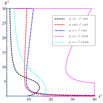
Figure 2: Contours of equal 1-loop and tree-level absolute contributions to the momentum-space 2-point correlator $\langle(\sqrt{B}u^{0}-1)(\sqrt{B}u^{0}-1)\rangle$, for various $\mathrm{O}(1)$ values of $c$ and $f_{3}$.

V Discussion

Our results are a strong hint that there exists a consistent quantum theory of fluids. If so, it is of great interest to explore the physical predictions of the theory, and to see whether they are realized in real-world systems. We can already draw some inferences from the results derived here. The first of these is that Lorentz invariance is non-linearly realized in the quantum vacuum, just as it is in a classical fluid. This follows immediately from the occurrence of poles at $\omega=ck$ in the 2-point correlators (III). Furthermore, the linearly realized symmetries appear to be the same in the quantum theory as in the classical theory, viz. the diagonal euclidean subgroup of Poincaré$\times\mathrm{SDiff}$. The second is that vortex modes apparently do not propagate, in the sense that they do not appear as poles in correlators of observables. In hindsight this is no surprise, since propagating vortices would imply IR divergences. We stress, though, that the absence of vortex modes does not mean that our fluid EFT is nothing but a complicated reformulation of a superfluid. Indeed, it is already known that a superfluid and an ordinary fluid are inequivalent at $\hbar=0$ (although they are equivalent if there is no vorticity) Dubovsky et al. (2006), and it follows by continuity that fluids and superfluids must be inequivalent in general at $\hbar\neq 0$. It is tempting to conjecture, however, that both the conservation of vorticity and the equivalence between the zero-vorticity fluid and the superfluid are preserved at the quantum level; if so, we must look to quantum fluids with non-vanishing vorticity in order to see a departure from superfluid behaviour. One possible arena would be the study of the quanta corresponding to Kelvin waves Thomson (1880), viz. low-energy perturbations of vortex lines [Forarecentlagrangianderivationofthese; see]Endlich:2013dma, for which ‘Thomsons’ is the obvious moniker. More generally, it would be of interest to explore the quantum version of any of the myriad phenomena of classical fluids: surface waves, turbulence, shocks, &c.

Where can we hope to observe such phenomena? Classical fluid behaviour is typically observed in underlying systems that are in local thermodynamic equilibrium at finite temperature. To see quantum behaviour in such a system, we would need to somehow ensure that thermal fluctuations are negligible in the long-distance fluid modes, which are what we quantize here. Alternatively, perhaps the correspondence of the theory with a fluid at the classical level is a red herring. We have given evidence that there exists an EFT, based on simple field content and symmetries, with behaviour that is qualitatively novel. That is interesting enough in itself, and leads us to hope that Nature may choose to make use of it somewhere.

References

- Note (1) Those who read while in the bath will be able to verify this easily, by slowing stirring the water in circles of varying size.
- Landau (1941a) L. D. Landau, Phys. Rev. 60, 356 (1941a).
- Landau (1941b) L. D. Landau, J. Phys. USSR 5, 71 (1941b).
- Endlich et al. (2011) S. Endlich, A. Nicolis, R. Rattazzi, and J. Wang, JHEP 1104, 102 (2011), arXiv:1011.6396 [hep-th] .
- Note (2) In fact, Endlich et al. focussed on the consequent breakdown of unitarity; it seems to us that the divergence of tree-level -matrix elements is a more fundamental problem per se.
- Note (3) Considering invariants was suggested in Endlich et al. (2011), but was not followed up.
- Note (4) If is a torus, for example, this can be arranged by ensuring that the Fourier modes above the EFT cut-off fall off faster than any polynomial.
- Khesin and Wendt (2009) B. Khesin and R. Wendt, The Geometry of Infinite-Dimensional Groups, A Series of Modern Surveys in Mathematics, Vol. 51 (Springer-Verlag, 2009).
- Endlich et al. (2013) S. Endlich, A. Nicolis, R. A. Porto, and J. Wang, Phys. Rev. D88, 105001 (2013), arXiv:1211.6461 [hep-th] .
- Herglotz (1911) G. Herglotz, Ann. Phy. 36, 493 (1911).
- Ballesteros and Bellazzini (2013) G. Ballesteros and B. Bellazzini, JCAP 1304, 001 (2013), arXiv:1210.1561 [hep-th] .
- Soper (2008) D. Soper, Classical Field Theory (Dover, 2008).
- Coleman (1973) S. R. Coleman, Commun. Math. Phys. 31, 259 (1973).
- Jevicki (1977) A. Jevicki, Phys. Lett. B71, 327 (1977).
- Elitzur (1983) S. Elitzur, Nucl. Phys. B212, 501 (1983).
- McKane and Stone (1980) A. McKane and M. Stone, Nucl. Phys. B163, 169 (1980).
- David (1980) F. David, Phys. Lett. B96, 371 (1980).
- David (1981) F. David, Commun. Math. Phys. 81, 149 (1981).
- Note (5) These quantities are not all Poincaré invariant, so they are still really only proxies for observables.
- Anastasiou and Lazopoulos (2004) C. Anastasiou and A. Lazopoulos, JHEP 0407, 046 (2004), arXiv:hep-ph/0404258 [hep-ph] .
- (21) J. A. M. Vermaseren, math-ph/0010025 .
- Dubovsky et al. (2006) S. Dubovsky, T. Gregoire, A. Nicolis, and R. Rattazzi, JHEP 0603, 025 (2006), arXiv:hep-th/0512260 [hep-th] .
- Thomson (1880) W. Thomson, Phil. Mag. 10, 155 (1880).
- Endlich and Nicolis (2013) S. Endlich and A. Nicolis, (2013), arXiv:1303.3289 [hep-th] .
- Martín-García et al. (2007) J. M. Martín-García, R. Portugal, and L. R. U. Manssur, Comp. Phys. Commun. 177, 640 (2007), arXiv:0704.1756 .