Confidence Corridors for Multivariate Generalized Quantile Regression

Abstract

We focus on the construction of confidence corridors for multivariate nonparametric generalized quantile regression functions. This construction is based on asymptotic results for the maximal deviation between a suitable nonparametric estimator and the true function of interest which follow after a series of approximation steps including a Bahadur representation, a new strong approximation theorem and exponential tail inequalities for Gaussian random fields.

As a byproduct we also obtain confidence corridors for the regression function in the classical mean regression. In order to deal with the problem of slowly decreasing error in coverage probability of the asymptotic confidence corridors, which results in meager coverage for small sample sizes, a simple bootstrap procedure is designed based on the leading term of the Bahadur representation. The finite sample properties of both procedures are investigated by means of a simulation study and it is demonstrated that the bootstrap procedure considerably outperforms the asymptotic bands in terms of coverage accuracy. Finally, the bootstrap confidence corridors are used to study the efficacy of the National Supported Work Demonstration, which is a randomized employment enhancement program launched in the 1970s. This article has supplementary materials online.

Keywords: Bootstrap; Expectile regression; Goodness-of-fit tests; Quantile treatment effect; Smoothing and nonparametric regression.
JEL: C2, C12, C14

1.  Introduction

Mean regression analysis is a widely used tool in statistical inference for curves. It focuses on the center of the conditional distribution, given $d$-dimensional covariates with $d\geq 1$. In a variety of applications though the interest is more in tail events, or even tail event curves such as the conditional quantile function. Applications with a specific demand in tail event curve analysis include finance, climate analysis, labor economics and systemic risk management.

Tail event curves have one thing in common: they describe the likeliness of extreme events conditional on the covariate $X$. A traditional way of defining such a tail event curve is by translating ”likeliness” with ”probability” leading to conditional quantile curves. Extreme events may alternatively be defined through conditional moment behaviour leading to more general tail descriptions as studied by Newey and Powell (1987) and Jones (1994). We employ this more general definition of generalized quantile regression (GQR), which includes, for instance, expectile curves and study statistical inference of GQR curves through confidence corridors.

In applications parametric forms are frequently used because of practical numerical reasons. Efficient algorithms are available for estimating the corresponding curves. However, the ”monocular view” of parametric inference has turned out to be too restrictive. This observation prompts the necessity of checking the functional form of GQR curves. Such a check may be based on testing different kinds of variation between a hypothesized (parametric) model and a smooth alternative GQR. Such an approach though involves either an explicit estimate of the bias or a pre-smoothing of the ”null model”. In this paper we pursue the Kolmogorov-Smirnov type of approach, that is, employing the maximal deviation between the null and the smooth GQR curve as a test statistic. Such a model check has the advantage that it may be displayed graphically as a confidence corridor (CC; also called ”simultaneous confidence band” or ”uniform confidence band/region”) but has been considered so far only for univariate covariates. The basic technique for constructing CC of this type is extreme value theory for the sup-norm of an appropriately centered nonparametric estimate of the quantile curve.

Confidence corridors with one-dimensional predictor were developed under various settings. Classical one-dimensional results are confidence bands constructed for histogram estimators by Smirnov (1950) or more general one-dimensional kernel density estimators by Bickel and Rosenblatt (1973). The results were extended to a univariate nonparametric mean regression setting by Johnston (1982), followed by Härdle (1989) who derived CCs for one-dimensional kernel $M$-estimators. Claeskens and Van Keilegom (2003) proposed uniform confidence bands and a bootstrap procedure for regression curves and their derivatives.

In recent years, the growth of the literature body shows no sign of decelerating. In the same spirit of Härdle (1989), Härdle and Song (2010) and Guo and Härdle (2012) constructed uniform confidence bands for local constant quantile and expectile curves. Fan and Liu (2013) proposed an integrated approach for building simultaneous confidence band that covers semiparametric models. Giné and Nickl (2010) investigated adaptive density estimation based on linear wavelet and kernel density estimators and Lounici and Nickl (2011) extended the framework of Bissantz et al. (2007) to adaptive deconvolution density estimation. Bootstrap procedures are proposed as a remedy for the poor coverage performance of asymptotic confidence corridors. For example, the bootstrap for the density estimator is proposed in Hall (1991) and Mojirsheibani (2012), and for local constant quantile estimators in Song et al. (2012).

However, only recently progress has been achieved in the construction of confidence bands for regression estimates with a multivariate predictor. Hall and Horowitz (2013) derived an expansion for the bootstrap bias and established a somewhat different way to construct confidence bands without the use of extreme value theory. Their bands are uniform with respect to a fixed but unspecified portion (smaller than one) of points in a possibly multidimensional set in contrast to the classical approach where uniformity is achieved on the complete set considered. Proksch et al. (2014) proposed multivariate confidence bands for convolution type inverse regression models with fixed design.

To the best of our knowledge, the classical Smirnov-Bickel-Rosenblatt type confidence corridors are not available for multivariate GQR or mean regression with random design.

In this work we go beyond the earlier studies in three aspects. First, we extend the applicability of the CC to $d$-dimensional covariates with $d>1$. Second, we present a more general approach covering not only quantile or mean curves but also GQR curves that are defined via a minimum contrast principle. Third, we propose a bootstrap procedure and we show numerically its improvement in the coverage accuracy as compared to the asymptotic approach.

Our asymptotic results, which describe the maximal absolute deviation of generalized quantile estimators, can not only be used to derive a goodness-of-fit test in quantile and expectile regression, but they are also applicable in testing the quantile treatment effect and stochastic dominance. We apply the new method to test the quantile treatment effect of the National Supported Work Demonstration program, which is a randomized employment enhancement program launched in the 1970s. The data associated with the participants of the program have been widely applied for treatment effect research since the pioneering study of LaLonde (1986). More recently, Delgado and Escanciano (2013) found that the program is beneficial for individuals of over 21 years of age. In our study, we find that the treatment tends to do better at raising the upper bounds of the earnings growth than raising the lower bounds. In other words, the program tends to increase the potential for high earnings growth but does not reduce the risk of negative earnings growth. The finding is particularly evident for those individuals who are older and spent more years at school. We should note that the tests based on the unconditional distribution cannot unveil the heterogeneity in the earnings growth quantiles in treatment effects.

The remaining part of this paper is organized as follows. In Section 2 we present our model, describe the estimators and state our asymptotic results. Section 3 is devoted to the bootstrap and we discuss its theoretical and practical aspects. The finite sample properties of both methods are investigated by means of a simulation study in Section 4, where we also compare the numerical performance of our method with the method proposed in Hall and Horowitz (2013) via simulations. The application of our new method is illustrated by a real data example in Section 5. The assumptions for our asymptotic theory are listed and discussed after the references. All detailed proofs are available in the supplement material.

2.  Asymptotic confidence corridors

In Section 2.1 we present the prerequisites such as the precise definition of the model and a suitable estimate. The result on constructing confidence corridors (CCs) based on the distribution of the maximal absolute deviation are given in Section 2.2. In Section 2.3 we describe how to estimate the scaling factors, which appear in the limit theorems, using residual based estimators. Section 3.1 introduce a new bootstrap method for constructing CCs, while Section 3.2 is devoted to specific issues related to bootstrap CCs for quantile regression. Assumptions are listed and discussed after the references.

2.1.  Prerequisites

Let $({\mbox{\boldmath$X$}}_{1},Y_{1}),...,({\mbox{\boldmath$X$}}_{n},Y_{n})$ be a sequence of independent identically distributed random vectors in $\mathbb{R}^{d+1}$ and consider the nonparametric regression model

$$Y_{i}=\theta_{0}({\mbox{\boldmath$X$}}_{i})+\varepsilon_{i},\quad i=1,...,n,$$ (1)

where $\theta_{0}$ is an aspect of $Y$ conditional on $X$, such as the $\tau$-quantile, the $\tau$-expectile or the mean regression curve, and the model errors $\varepsilon_{1},\ldots,\varepsilon_{n}$ are i.i.d. with $\tau$-quantile, $\tau$-expectile or mean equal to 0, respectively, depending on which $\theta_{0}$ is in the model. The function $\theta({\mbox{\boldmath$x$}})$ can be estimated by:

$$\hat{\theta}({\mbox{\boldmath$x$}})=\operatorname*{arg\,min}_{\theta\in\mathbb{R}}\frac{1}{n}\sum_{i=1}^{n}K_{h}({\mbox{\boldmath$x$}}-{\mbox{\boldmath$X$}}_{i})\rho(Y_{i}-\theta),$$ (2)

where $K_{h}({\mbox{\boldmath$u$}})=h^{-d}K\left({\mbox{\boldmath$u$}}/h\right)$ for some kernel function $K:\mathbb{R}^{d}\rightarrow\mathbb{R}$, and a loss-function $\rho_{\tau}:\mathbb{R}\rightarrow\mathbb{R}$. In this paper we are concerned with the construction of uniform confidence corridors for quantile as well as expectile regression curves when the predictor is multivariate, that is, we focus on the loss functions

$$\rho_{\tau}(u)=\big{|}\bm{1}(u<0)-\tau\big{|}|u|^{k},$$

for $k=1$ and 2 associated with quantile and expectile regression. We derive the asymptotic distribution of the properly scaled maximal deviation $\sup_{{\mbox{\scriptsize\boldmath$x$}}\in\mathcal{D}}|\hat{\theta}_{n}({\mbox{\boldmath$x$}})-\theta({\mbox{\boldmath$x$}})|$ for both cases, where $\mathcal{D}\subset\mathbb{R}^{d}$ is a compact subset. We use strong approximations of the empirical process, concentration inequalities for general Gaussian random fields and results from extreme value theory. To be precise, we show that

$$\mathrm{P}\left[(2\delta\log n)^{1/2}\Big{\{}\sup_{{\mbox{\scriptsize\boldmath$x$}}\in\mathcal{D}}\big{|}r_{n}({\mbox{\boldmath$x$}})\big{[}\hat{\theta}_{n}({\mbox{\boldmath$x$}})-\theta_{0}({\mbox{\boldmath$x$}})\big{]}\big{|}/\|K\|_{2}-d_{n}\Big{\}}<a\right]\rightarrow\exp\big{\{}-2\exp(-a)\big{\}},$$ (3)

as $n\rightarrow\infty$, where $r_{n}({\mbox{\boldmath$x$}})$ is a scaling factor which depends on $x$, $n$ and the loss function under consideration.

2.2.  Asymptotic results

In this section we present our main theoretical results on the distribution of the uniform maximal deviation of the quantile and expectile estimator. The proofs of the theorems at their full lengths are deferred to the appendix. Here we only give a brief sketch of proof of Theorem 2.1 which is the limit theorem for the case of quantile regression.

THEOREM 2.1.

Let $\hat{\theta}_{n}({\mbox{\boldmath$x$}})$ and $\theta_{0}({\mbox{\boldmath$x$}})$ be the local constant quantile estimator and the true quantile function, respectively and suppose that assumptions (A1)-(A6) in Section A hold. Let further $\mbox{vol}(\mathcal{D})=1$ and

$$d_{n}=(2d\kappa\log n)^{1/2}+\big{\{}2d\kappa(\log n)\big{\}}^{-1/2}\left[\frac{1}{2}(d-1)\log\log n^{\kappa}+\log\big{\{}(2\pi)^{-1/2}H_{2}(2d)^{(d-1)/2}\big{\}}\right],$$

where $H_{2}=\big{(}2\pi\|K\|_{2}^{2}\big{)}^{-d/2}\det(\Sigma)^{1/2},\mbox{ }\Sigma=\bigl{(}\Sigma_{ij}\bigr{)}_{1\leq i,j\leq d}=\Bigl{(}\int\frac{\partial K({\mbox{\scriptsize\boldmath$u$}})}{\partial u_{i}}\frac{\partial K({\mbox{\scriptsize\boldmath$u$}})}{\partial u_{j}}d{\mbox{\scriptsize\boldmath$u$}}\Bigr{)}_{1\leq i,j\leq d},$

$$r_{n}({\mbox{\boldmath$x$}})=\sqrt{\frac{nh^{d}f_{\mbox{\scriptsize\boldmath$X$}}({\mbox{\boldmath$x$}})}{\tau(1-\tau)}}f_{Y|{\mbox{\scriptsize\boldmath$X$}}}\big{\{}\theta_{0}({\mbox{\boldmath$x$}})|{\mbox{\boldmath$x$}}\big{\}},$$

Then the limit theorem (3) holds.

Sketch of proof. A major technical difficulty is imposed by the fact that the loss-function $\rho_{\tau}$ is not smooth which means that standard arguments such as those based on Taylor’s theorem do not apply. As a consequence the use of a different, extended methodology becomes necessary. In this context Kong et al. (2010) derived a uniform Bahadur representation for an $M$-regression function in a multivariate setting (see appendix). It holds uniformly for $x\in\mathcal{D}$, where $\mathcal{D}$ is a compact subset of $\mathbb{R}^{d}$:

$$\hat{\theta}_{n}({\mbox{\boldmath$x$}})-\theta_{0}({\mbox{\boldmath$x$}})=\frac{1}{nS_{n,0,0}({\mbox{\boldmath$x$}})}\sum_{i=1}^{n}K_{h}({\mbox{\boldmath$x$}}-{\mbox{\boldmath$X$}}_{i})\psi_{\tau}\big{\{}Y_{i}-\theta_{0}({\mbox{\boldmath$x$}})\big{\}}+\mathcal{O}\left\{\Big{(}\frac{\log n}{nh^{d}}\Big{)}^{\frac{3}{4}}\right\},\quad a.s.$$ (4)

Here $S_{n,0,0}({\mbox{\boldmath$x$}})=\int K({\mbox{\boldmath$u$}})g({\mbox{\boldmath$x$}}+h{\mbox{\boldmath$u$}})f_{\mbox{\scriptsize\boldmath$X$}}({\mbox{\boldmath$x$}}+h{\mbox{\boldmath$u$}})d{\mbox{\boldmath$u$}}$, $\psi_{\tau}(u)=\bm{1}(u<0)-\tau$ is the piecewise derivative of the loss-function $\rho_{\tau}$ and

$$g({\mbox{\boldmath$x$}}) =\left.\frac{\partial}{\partial t}\mbox{\sf E}[\psi_{\tau}(Y-t)|{\mbox{\boldmath$X$}}={\mbox{\boldmath$x$}}]\right|_{t=\theta_{0}({\mbox{\scriptsize\boldmath$x$}})}.$$

Notice that the error term of the Bahadur expansion does not depend on the design $X$ and it converges to 0 with rate $\big{(}\log n/nh^{d}\big{)}^{\frac{3}{4}}$ which is much faster than the convergence rate $(nh^{d})^{-\frac{1}{2}}$ of the stochastic term.

Rearranging (4), we obtain

$$S_{n,0,0}({\mbox{\boldmath$x$}})\{\hat{\theta}_{n}({\mbox{\boldmath$x$}})-\theta_{0}({\mbox{\boldmath$x$}})\}=\frac{1}{n}\sum_{i=1}^{n}K_{h}({\mbox{\boldmath$x$}}-{\mbox{\boldmath$X$}}_{i})\psi_{\tau}\big{\{}Y_{i}-\theta_{0}({\mbox{\boldmath$x$}})\big{\}}+\mathcal{O}\left\{\Big{(}\frac{\log n}{nh^{d}}\Big{)}^{\frac{3}{4}}\right\}.$$ (5)

Now we express the leading term on the right hand side of (5) by means of the centered empirical process

$$Z_{n}(y,{\mbox{\boldmath$u$}})=n^{1/2}\{F_{n}(y,{\mbox{\boldmath$u$}})-F(y,{\mbox{\boldmath$u$}})\},$$ (6)

where $F_{n}(y,{\mbox{\boldmath$x$}})=n^{-1}\sum_{i=1}^{n}\bm{1}(Y_{i}\leq y,X_{i1}\leq x_{1},...,X_{id}\leq x_{d})$. This yields, by Fubini’s theorem,

$$S_{n,0,0}({\mbox{\boldmath$x$}})\{\hat{\theta}_{n}({\mbox{\boldmath$x$}})-\theta_{0}({\mbox{\boldmath$x$}})\}-b({\mbox{\boldmath$x$}})=n^{-1/2}\int\int K_{h}({\mbox{\boldmath$x$}}-{\mbox{\boldmath$u$}})\psi_{\tau}\big{\{}y-\theta_{0}({\mbox{\boldmath$x$}})\big{\}}dZ_{n}(y,{\mbox{\boldmath$u$}})+\mathcal{O}\left\{\Big{(}\frac{\log n}{nh^{d}}\Big{)}^{\frac{3}{4}}\right\},$$ (7)

where

$$b({\mbox{\boldmath$x$}})=-\mbox{\sf E}_{\mbox{\scriptsize\boldmath$x$}}\left[\frac{1}{n}\sum_{i=1}^{n}K_{h}({\mbox{\boldmath$x$}}-{\mbox{\boldmath$X$}}_{i})\psi\big{\{}Y_{i}-\theta_{0}({\mbox{\boldmath$x$}})\big{\}}\right]$$

denotes the bias which is of order $\mathcal{O}(h^{s})$ by Assumption (A3) in the Appendix. The variance of the first term of the right hand side of (7) can be estimated via a change of variables and Assumption (A5), which gives

$$(nh^{d})^{-2}n\mbox{\sf E}\big{[}K^{2}\big{\{}({\mbox{\boldmath$x$}}-{\mbox{\boldmath$X$}}_{i})/h\big{\}}\psi^{2}\big{\{}Y_{i}-\theta_{0}({\mbox{\boldmath$x$}})\big{\}}\big{]}$$

$$=(nh^{d})^{-2}nh^{d}\int\int K^{2}({\mbox{\boldmath$v$}})\psi^{2}\big{\{}y-\theta_{0}({\mbox{\boldmath$x$}})\big{\}}f_{Y|{\mbox{\scriptsize\boldmath$X$}}}(y|{\mbox{\boldmath$x$}}-h{\mbox{\boldmath$v$}})f_{\mbox{\scriptsize\boldmath$X$}}({\mbox{\boldmath$x$}}-h{\mbox{\boldmath$v$}})dyd{\mbox{\boldmath$v$}}$$

$$=(nh^{d})^{-1}\int\int K^{2}({\mbox{\boldmath$v$}})\psi^{2}\big{\{}y-\theta_{0}({\mbox{\boldmath$x$}})\big{\}}f_{Y|{\mbox{\scriptsize\boldmath$X$}}}(y|{\mbox{\boldmath$x$}})f_{\mbox{\scriptsize\boldmath$X$}}({\mbox{\boldmath$x$}})dyd{\mbox{\boldmath$v$}}+\mathcal{O}\big{(}(nh^{d-1})^{-1}\big{)}$$

$$=(nh^{d})^{-1}f_{\mbox{\scriptsize\boldmath$X$}}({\mbox{\boldmath$x$}})\sigma^{2}({\mbox{\boldmath$x$}})\|K\|_{2}^{2}+\mathcal{O}\big{\{}(nh^{d})^{-1}h\big{\}},$$

where $\sigma^{2}({\mbox{\boldmath$x$}})=\mbox{\sf E}[\psi^{2}\big{\{}Y-\theta_{0}({\mbox{\boldmath$x$}})\big{\}}|{\mbox{\boldmath$X$}}={\mbox{\boldmath$x$}}]$. The standardized version of (5) can therefore be approximated by

$$\frac{\sqrt{nh^{d}}}{\sqrt{f_{\mbox{\scriptsize\boldmath$X$}}({\mbox{\boldmath$x$}})}\sigma({\mbox{\boldmath$x$}})\|K\|_{2}}S_{n,0,0}({\mbox{\boldmath$x$}})\{\hat{\theta}_{n}({\mbox{\boldmath$x$}})-\theta_{0}({\mbox{\boldmath$x$}})\}$$

$$=\frac{1}{\sqrt{h^{d}f_{\mbox{\scriptsize\boldmath$X$}}({\mbox{\boldmath$x$}})}\sigma({\mbox{\boldmath$x$}})\|K\|_{2}}\int\int K\left(\frac{{\mbox{\boldmath$x$}}-{\mbox{\boldmath$u$}}}{h}\right)\psi\big{\{}Y_{i}-\theta_{0}({\mbox{\boldmath$x$}})\big{\}}dZ_{n}(y,{\mbox{\boldmath$u$}})+\mathcal{O}\big{(}\sqrt{nh^{d}}h^{s}\big{)}+\mathcal{O}\left\{\Big{(}\frac{\log n}{nh^{d}}\Big{)}^{\frac{3}{4}}\right\}.$$ (8)

The dominating term is defined by

$$Y_{n}({\mbox{\boldmath$x$}})\stackrel{{\scriptstyle\mathrm{def}}}{{=}}\frac{1}{\sqrt{h^{d}f_{\mbox{\scriptsize\boldmath$X$}}({\mbox{\boldmath$x$}})}\sigma({\mbox{\boldmath$x$}})}\int\int K\left(\frac{{\mbox{\boldmath$x$}}-{\mbox{\boldmath$u$}}}{h}\right)\psi\big{\{}y-\theta_{0}({\mbox{\boldmath$x$}})\big{\}}dZ_{n}(y,{\mbox{\boldmath$u$}}).$$ (9)

Involving strong Gaussian approximation and Bernstein-type concentration inequalities, this process can be approximated by a stationary Gaussian field:

$$Y_{5,n}({\mbox{\boldmath$x$}})=\frac{1}{\sqrt{h^{d}}}\int K\left(\frac{{\mbox{\boldmath$x$}}-{\mbox{\boldmath$u$}}}{h}\right)dW\big{(}{\mbox{\boldmath$u$}}\big{)},$$ (10)

where $W$ denotes a Brownian sheet. The supremum of this process is asymptotically Gumbel distributed, which follows, e.g., by Theorem 2 of Rosenblatt (1976). Since the kernel is symmetric and of order $s$, we can estimate the term

$$S_{n,0,0}=f_{Y|{\mbox{\scriptsize\boldmath$X$}}}(\theta_{0}({\mbox{\boldmath$x$}})|{\mbox{\boldmath$x$}})f_{\mbox{\scriptsize\boldmath$X$}}({\mbox{\boldmath$x$}})+\mathcal{O}(h^{s})$$

if (A5) holds. On the other hand, $\sigma^{2}({\mbox{\boldmath$x$}})=\tau(1-\tau)$ in quantile regression. Therefore, the statements of the theorem hold.

$\Box$

Corollary 2.2 (CC for multivariate quantile regression).

Under the assumptions of Theorem 2.1, an approximate $(1-\alpha)\times 100\%$ confidence corridor is given by

$$\hat{\theta}_{n}({\mbox{\boldmath$t$}})\pm(nh^{d})^{-1/2}\big{\{}\tau(1-\tau)\|K\|_{2}/\hat{f}_{\mbox{\scriptsize\boldmath$X$}}({\mbox{\boldmath$t$}})\big{\}}^{1/2}\hat{f}_{\varepsilon|{\mbox{\scriptsize\boldmath$X$}}}\big{\{}0|{\mbox{\boldmath$t$}}\big{\}}^{-1}\Big{\{}d_{n}+c(\alpha)(2\kappa d\log n)^{-1/2}\Big{\}},$$

where $\alpha\in(0,1)$ and $c(\alpha)=\log 2-\log\big{|}\log(1-\alpha)\big{|}$ and $\hat{f}_{\mbox{\scriptsize\boldmath$X$}}({\mbox{\boldmath$t$}})$, $\hat{f}_{\varepsilon|{\mbox{\scriptsize\boldmath$X$}}}\big{\{}0|{\mbox{\boldmath$t$}}\big{\}}$ are consistent estimates for $f_{\mbox{\scriptsize\boldmath$X$}}({\mbox{\boldmath$t$}})$, $f_{\varepsilon|{\mbox{\scriptsize\boldmath$X$}}}\big{\{}0|{\mbox{\boldmath$t$}}\big{\}}$ with convergence rate in sup-norm faster than ${\scriptstyle{\mathcal{O}}}_{p}\big{(}(\log n)^{-1/2}\big{)}$.

Remark 2.3.

Note that under the conditions of Corollary 2.2 we find

$$\sup_{{\mbox{\scriptsize\boldmath$x$}}\in\mathcal{D}}\bigl{|}r_{n}({\mbox{\boldmath$x$}})\bigl{(}\hat{\theta}_{n}({\mbox{\boldmath$x$}})-\theta_{0}({\mbox{\boldmath$x$}}))\bigr{)}\bigr{|}=\mathcal{O}_{P}\bigl{(}\sqrt{\log(n)}\bigr{)},$$

where

$$r_{n}({\mbox{\boldmath$x$}})=\sqrt{\frac{nh^{d}f_{\mbox{\scriptsize\boldmath$X$}}({\mbox{\boldmath$x$}})}{\tau(1-\tau)}}f_{Y|{\mbox{\scriptsize\boldmath$X$}}}\big{\{}\theta_{0}({\mbox{\boldmath$x$}})|{\mbox{\boldmath$x$}}\big{\}}.$$

For kernel estimators $\hat{f}_{\varepsilon|{\mbox{\scriptsize\boldmath$X$}}}(0,\cdot)$ and $\hat{f}_{{\mbox{\scriptsize\boldmath$X$}}}(\cdot)$ converging in sup-norm with rate ${\scriptstyle{\mathcal{O}}}_{P}\bigl{(}\log(n)^{-1/2}\Bigr{)}$ to $f_{\varepsilon|{\mbox{\boldmath$X$}}}(0,\cdot)$ and $f_{{\mbox{\boldmath$X$}}}(\cdot)$, respectively, the quantity $\hat{r}_{n}({\mbox{\boldmath$x$}})$, defined by

$$\hat{r}_{n}({\mbox{\boldmath$x$}})=\sqrt{\frac{nh^{d}\hat{f}_{\mbox{\scriptsize\boldmath$X$}}({\mbox{\boldmath$x$}})}{\tau(1-\tau)}}\hat{f}_{\varepsilon|{\mbox{\scriptsize\boldmath$X$}}}(0,{\mbox{\boldmath$x$}}),$$

inherits this rate. Furthermore, since we consider an additive error model, the conditional density $f_{Y|{\mbox{\scriptsize\boldmath$X$}}}\big{\{}\theta_{0}({\mbox{\boldmath$x$}})|{\mbox{\boldmath$x$}}\big{\}}$ can be replaced by $f_{\varepsilon|{\mbox{\scriptsize\boldmath$X$}}}(0,{\mbox{\boldmath$x$}})$ (see Section 2.3 below for more details and the definition of suitable estimators). This yields

$$\sup_{{\mbox{\scriptsize\boldmath$x$}}\in\mathcal{D}}\bigl{|}\hat{r}_{n}({\mbox{\boldmath$x$}})\bigl{(}\hat{\theta}_{n}({\mbox{\boldmath$x$}})-\theta_{0}({\mbox{\boldmath$x$}}))\bigr{)}\bigr{|}={\scriptstyle{\mathcal{O}}}_{P}(1)+\sup_{{\mbox{\scriptsize\boldmath$x$}}\in\mathcal{D}}\bigl{|}r_{n}({\mbox{\boldmath$x$}})\bigl{(}\hat{\theta}_{n}({\mbox{\boldmath$x$}})-\theta_{0}({\mbox{\boldmath$x$}}))\bigr{)}\bigr{|}.$$

Hence, by Slutsky’s Lemma, the quantities $\sup_{{\mbox{\scriptsize\boldmath$x$}}\in\mathcal{D}}\bigl{|}\hat{r}_{n}({\mbox{\boldmath$x$}})\bigl{(}\hat{\theta}_{n}({\mbox{\boldmath$x$}})-\theta_{0}({\mbox{\boldmath$x$}}))\bigr{)}\bigr{|}$ and $\sup_{{\mbox{\scriptsize\boldmath$x$}}\in\mathcal{D}}\bigl{|}r_{n}({\mbox{\boldmath$x$}})\bigl{(}\hat{\theta}_{n}({\mbox{\boldmath$x$}})-\theta_{0}({\mbox{\boldmath$x$}}))\bigr{)}\bigr{|}$ have the same asymptotic distribution.

The expectile confidence corridor can be constructed in an analogous manner as the quantile confidence corridor. The two cases differ in the form and hence the properties of the loss function. Therefore we find for expectile regression:

$$S_{n,0,0}({\mbox{\boldmath$x$}})=-2\big{[}F_{Y|{\mbox{\scriptsize\boldmath$X$}}}\big{(}\theta_{0}({\mbox{\boldmath$x$}}\big{)}|{\mbox{\boldmath$x$}})(2\tau-1)-\tau\big{]}f_{\mbox{\scriptsize\boldmath$X$}}({\mbox{\boldmath$x$}})+\mathcal{O}(h^{s}).$$

Through similar approximation steps as the quantile regression, we derive the following theorem.

THEOREM 2.4.

Let $\hat{\theta}_{n}({\mbox{\boldmath$x$}})$ be the the local constant expectile estimator and $\theta_{0}({\mbox{\boldmath$x$}})$ the true expectile function. If Assumptions (A1), (A3)-(A6) and (EA2) of Section A hold with a constant $b_{1}$ satisfying

$$n^{-1/6}h^{-d/2-3d/(b_{1}-2)}=\mathcal{O}(n^{-\nu}),\quad\nu>0.$$

Then the limit theorem (3) holds with a scaling factor

$$r_{n}({\mbox{\boldmath$x$}})=\sqrt{nh^{d}f_{\mbox{\scriptsize\boldmath$X$}}({\mbox{\boldmath$x$}})}\sigma^{-1}({\mbox{\boldmath$x$}})\left\{2\big{[}\tau-F_{Y|{\mbox{\scriptsize\boldmath$X$}}}(\theta_{0}({\mbox{\boldmath$x$}})|{\mbox{\boldmath$x$}})(2\tau-1)\big{]}\right\}$$

and with the same constants $H_{2}$ and $d_{n}$ as defined in Theorem 2.1, where $\sigma^{2}({\mbox{\boldmath$x$}})=\mbox{\sf E}[\psi_{\tau}^{2}(Y-\theta_{0}({\mbox{\boldmath$x$}}))|{\mbox{\boldmath$X$}}={\mbox{\boldmath$x$}}]$ and $\psi_{\tau}(u)=2(\bm{1}(u\leq 0)-\tau)|u|$ is the derivative of the expectile loss-function $\rho_{\tau}(u)=\big{|}\tau-\bm{1}(u<0)\big{|}|u|^{2}$.

The proof of this result is deferred to the appendix. In the next corollary, the explicit form of the CCs for expectiles is given.

Corollary 2.5 (CC for multivariate expectile regression).

Under the same assumptions of Theorem 2.4, an approximate $(1-\alpha)\times 100\%$ confidence corridor is given by

$$\hat{\theta}_{n}({\mbox{\boldmath$t$}})\pm(nh^{d})^{-1/2}\big{\{}\hat{\sigma}^{2}({\mbox{\boldmath$t$}})\|K\|_{2}/\hat{f}_{\mbox{\scriptsize\boldmath$X$}}({\mbox{\boldmath$t$}})\big{\}}^{1/2} \Big{\{}-2\big{[}\hat{F}_{\varepsilon|{\mbox{\scriptsize\boldmath$X$}}}\big{\{}0|{\mbox{\boldmath$t$}}\big{\}}(2\tau-1)-\tau\big{]}\Big{\}}^{-1}\Big{\{}d_{n}+c(\alpha)(2\kappa d\log n)^{-1/2}\Big{\}},$$

where $\alpha\in(0,1)$ $c(\alpha)=\log 2-\log\big{|}\log(1-\alpha)\big{|}$ and $\hat{f}_{\mbox{\scriptsize\boldmath$X$}}({\mbox{\boldmath$t$}})$, $\hat{\sigma}^{2}({\mbox{\boldmath$t$}})$ and $\hat{F}_{\varepsilon|{\mbox{\scriptsize\boldmath$X$}}}(0|{\mbox{\boldmath$x$}})$ are consistent estimates for $f_{\mbox{\scriptsize\boldmath$X$}}({\mbox{\boldmath$t$}})$, $\sigma^{2}({\mbox{\boldmath$t$}})$ and $F_{\varepsilon|{\mbox{\scriptsize\boldmath$X$}}}(0|{\mbox{\boldmath$x$}})$ with convergence rate in sup-norm faster than ${\scriptstyle{\mathcal{O}}}_{p}\big{(}(\log n)^{-1/2}\big{)}$.

A further immediate consequence of Theorem 2.4 is a similar limit theorem in the context of local least squares estimation of the regression curve in classical mean regression.

Corollary 2.6 (CC for multivariate mean regression).

Consider the loss function $\rho(u)=u^{2}$ corresponding to $\psi(u)=2u.$ Under the assumptions of Theorem 2.4, with the same constants $H_{2}$ and $d_{n}$, (3) holds for the local constant estimator $\hat{\theta}$ and the regression function $\theta(x)=E[Y\,|\,{\mbox{\boldmath$X$}}={\mbox{\boldmath$x$}}]$ with scaling factor $r({\mbox{\boldmath$x$}})=\sqrt{nh^{d}f_{\mbox{\scriptsize\boldmath$X$}}({\mbox{\boldmath$x$}})}\sigma^{-1}({\mbox{\boldmath$x$}})$ and $\sigma^{2}({\mbox{\boldmath$x$}})=$Var$[Y\,|\,{\mbox{\boldmath$X$}}={\mbox{\boldmath$x$}}].$

Remark 2.7.

We would like to stress that our purely non-parametric approach offers flexibility and reasonable results in moderate dimensions $d=2,\,d=3$, but it is not suitable for inference in high dimensional models due to the curse of dimensionality. The case of high dimensional regressors may be handled via a semi-parametric specification of the regression curve, such as, for instance, a partial linear model. Such a model was considered in Song et al. (2012) with a one-dimensional non-parametric component. We think that our approach allows to adapt these ideas and, as an extension, to consider a non-parametric component which is multivariate. Hence, our approach then also offers higher flexibility in semi-parametric modeling. This semi-parametric approach is not pursued further in this paper but it clearly deserves future research.

2.3.  Estimating the scaling factors

The performance of the confidence bands is greatly influenced by the scaling factors $\hat{f}_{{\varepsilon}|{\mbox{\scriptsize\boldmath$X$}}}(v|{\mbox{\boldmath$x$}})$, $F_{{\varepsilon}|{\mbox{\scriptsize\boldmath$X$}}}(v|{\mbox{\boldmath$x$}})$ and $\hat{\sigma}({\mbox{\boldmath$x$}})^{2}$. The purpose of this subsection is thus to propose a way to estimate these factors and investigate their asymptotic properties.

As pointed out by our referee, estimating $f_{{\varepsilon}|{\mbox{\scriptsize\boldmath$X$}}}(0)$ is not a trivial task. The application of a rank test described in Chapter 3.5 of Koenker (2005) is an alternative to avoid estimating $f_{{\varepsilon}|{\mbox{\scriptsize\boldmath$X$}}}(0)$ in parametric quantile regression. However, it is a challenging task to apply this technique to kernel smoothing quantile regression. For pointwise nonparametric inference, it may be possible to construct a test by adding weights (given by $h^{-1}K(({\mbox{\boldmath$x$}}-{\mbox{\boldmath$X$}}_{i})/h)$, where $h$ is the bandwidth and $K$ is the kernel function) in the linear programing problem and therefore its dual can also be computed. However, a global shape test like the one investigated in this paper cannot be derived from the rank test. Hence, it seems inevitable to estimate the nuisance parameters and plug them into the test statistics.

Since we consider the additive error model (1), the conditional distribution function $F_{Y|{\mbox{\scriptsize\boldmath$X$}}}(\theta_{0}({\mbox{\boldmath$x$}})|{\mbox{\boldmath$x$}})$ and the conditional density $f_{Y|{\mbox{\scriptsize\boldmath$X$}}}(\theta_{0}({\mbox{\boldmath$x$}})|{\mbox{\boldmath$x$}})$ can be replaced by $F_{\varepsilon|{\mbox{\scriptsize\boldmath$X$}}}(0|{\mbox{\boldmath$x$}})$ and $f_{{\varepsilon}|{\mbox{\scriptsize\boldmath$X$}}}(0|{\mbox{\boldmath$x$}})$, respectively, where $F_{\varepsilon|{\mbox{\scriptsize\boldmath$X$}}}$ and $f_{\varepsilon|{\mbox{\scriptsize\boldmath$X$}}}$ are the conditional distribution and density functions of $\varepsilon$. Similarly, we have

$$\sigma^{2}({\mbox{\boldmath$x$}})=\mbox{\sf E}\big{[}\psi_{\tau}\big{(}Y-\theta_{0}({\mbox{\boldmath$x$}})\big{)}^{2}\big{|}{\mbox{\boldmath$X$}}={\mbox{\boldmath$x$}}\big{]}=\mbox{\sf E}\big{[}\psi_{\tau}(\varepsilon)^{2}\big{|}{\mbox{\boldmath$X$}}={\mbox{\boldmath$x$}}\big{]}$$

where ${\varepsilon}$ may depend on $X$ due to heterogeneity. It should be noted that the kernel estimators for $f_{{\varepsilon}|{\mbox{\scriptsize\boldmath$X$}}}(0|{\mbox{\boldmath$x$}})$ and $f_{Y|{\mbox{\scriptsize\boldmath$X$}}}(\theta_{0}({\mbox{\boldmath$x$}})|{\mbox{\boldmath$x$}})$ are asymptotically equivalent, but show different finite sample behavior. We explore this issue further in the following section.

Introducing the residuals $\hat{\varepsilon}_{i}=Y_{i}-\hat{\theta}_{n}({\mbox{\boldmath$X$}}_{i})$ we propose to estimate $F_{\varepsilon|{\mbox{\scriptsize\boldmath$X$}}}$, $f_{\varepsilon|{\mbox{\scriptsize\boldmath$X$}}}$ and $\sigma^{2}({\mbox{\boldmath$x$}})$ by

$$\hat{F}_{\varepsilon|{\mbox{\scriptsize\boldmath$X$}}}(v|{\mbox{\boldmath$x$}}) =n^{-1}\sum_{i=1}^{n}G\left(\frac{v-\hat{\varepsilon}_{i}}{h_{0}}\right)L_{\bar{h}}({\mbox{\boldmath$x$}}-{\mbox{\boldmath$X$}}_{i})/\hat{f}_{\mbox{\scriptsize\boldmath$X$}}({\mbox{\boldmath$x$}}),$$ (11)

$$\hat{f}_{\varepsilon|{\mbox{\scriptsize\boldmath$X$}}}(v|{\mbox{\boldmath$x$}}) =n^{-1}\sum_{i=1}^{n}g_{h_{0}}\left(v-\hat{\varepsilon}_{i}\right)L_{\bar{h}}({\mbox{\boldmath$x$}}-{\mbox{\boldmath$X$}}_{i})/\hat{f}_{\mbox{\scriptsize\boldmath$X$}}({\mbox{\boldmath$x$}}),$$ (12)

$$\hat{\sigma}^{2}({\mbox{\boldmath$x$}}) =n^{-1}\sum_{i=1}^{n}\psi^{2}(\hat{\varepsilon}_{i})L_{\bar{h}}({\mbox{\boldmath$x$}}-{\mbox{\boldmath$X$}}_{i})/\hat{f}_{\mbox{\scriptsize\boldmath$X$}}({\mbox{\boldmath$x$}}),$$ (13)

where $\hat{f}_{\mbox{\scriptsize\boldmath$X$}}({\mbox{\boldmath$x$}})=n^{-1}\sum_{i=1}^{n}L_{\bar{h}}({\mbox{\boldmath$x$}}-{\mbox{\boldmath$X$}}_{i})$, $G$ is a given continuously differentiable cumulative distribution function and $g$ is its derivative. The construction of estimators in (11) and (12) follows from the estimator for general conditional distribution and density functions discussed in Chapter 5 and 6 of Li and Racine (2007). The same bandwidth $\bar{h}$ is applied to the three estimators, but the choice of $\bar{h}$ will make the convergence rate of (13) sub-optimal. More details on the choice of $\bar{h}$ are given in section 3.2 below. Nevertheless, the rate of convergence of (13) is of polynomial order in $n$. The theory developed in this subsection can be generalized to the case of different bandwidth for different direction without much difficulty.

The estimators (11) and (12) belong to the family of residual-based estimators. The consistency of residual-based density estimators for errors in a regression model are explored in the literature in various settings. It is possible to obtain an expression for the residual based kernel density estimator as the sum of the estimator with the true residuals, the partial sum of the true residuals and a term for the bias of the nonparametrically estimated function, as shown in Muhsal and Neumeyer (2010), among others. The residual based conditional kernel density case is less considered in the literature. Kiwitt and Neumeyer (2012) consider the residual based kernel estimator for conditional distribution function conditioning on a one-dimensional variable.

Below we give consistency results for the estimators defined in (11), (12) and (13). The proof can be found in the appendix.

Lemma 2.8.

Under conditions (A1), (A3)-(A5), (B1)-(B3) in Section A, we have

1. $\sup_{v\in I}\sup_{{\mbox{\scriptsize\boldmath$x$}}\in\mathcal{D}}\big{|}\hat{F}_{\varepsilon|{\mbox{\scriptsize\boldmath$X$}}}(v|{\mbox{\boldmath$x$}})-F_{\varepsilon|{\mbox{\scriptsize\boldmath$X$}}}(v|{\mbox{\boldmath$x$}})\big{|}=\mathcal{O}_{p}\big{(}t_{n}\big{)}$,

2. $\sup_{v\in I}\sup_{{\mbox{\scriptsize\boldmath$x$}}\in\mathcal{D}}\big{|}\hat{f}_{\varepsilon|{\mbox{\scriptsize\boldmath$X$}}}(v|{\mbox{\boldmath$x$}})-f_{\varepsilon|{\mbox{\scriptsize\boldmath$X$}}}(v|{\mbox{\boldmath$x$}})\big{|}=\mathcal{O}_{p}\big{(}t_{n}\big{)}$,

3. $\sup_{{\mbox{\scriptsize\boldmath$x$}}\in\mathcal{D}}\big{|}\hat{\sigma}^{2}({\mbox{\boldmath$x$}})-\sigma^{2}({\mbox{\boldmath$x$}})\big{|}=\mathcal{O}_{p}\big{(}u_{n}\big{)}$,

where $t_{n}=\mathcal{O}\big{\{}h_{0}^{s^{\prime}}+h^{s}+\bar{h}^{s^{\prime}}+(n\bar{h}^{d})^{-1/2}\log n+(nh^{d})^{-1/2}\log n\big{\}}=\mathcal{O}(n^{-\lambda})$, and $u_{n}=\mathcal{O}\big{\{}h^{s}+\bar{h}^{s^{\prime}}+(n\bar{h}^{d})^{-1/2}\log n+(nh^{d})^{-1/2}\log n\big{\}}=\mathcal{O}(n^{-\lambda_{1}})$ for some constants $\lambda,\lambda_{1}>0$.

The factor of $\log n$ shown in the convergence rate is the price which we pay for the supnorm deviation. Since these estimators uniformly converge in a polynomial rate in $n$, the asymptotic distributions in Theorem 2.1 and 2.4 do not change if we plug these estimators into the formulae.

3.  Bootstrap confidence corridors

3.1.  Asymptotic theory

In the case of the suitably normed maximum of independent standard normal variables, it is shown in Hall (1979) that the speed of convergence in limit theorems of the form (3) is of order $1/\log n$, that is, the coverage error of the asymptotic CC decays only logarithmically. This leads to unsatisfactory finite sample performance of the asymptotic methods, especially for small sample sizes and dimensions $d>1$. However, Hall (1991) suggests that the use of a bootstrap method, based on a proper way of resampling, can increase the speed of shrinking of coverage error to a polynomial rate of $n$. In this section we therefore propose a specific bootstrap technique and construct a confidence corridor for the objects to be analysed.

Given the residuals $\hat{\varepsilon}_{i}=Y_{i}-\hat{\theta}_{n}({\mbox{\boldmath$X$}}_{i})$, the bootstrap observations $({\mbox{\boldmath$X$}}_{i}^{*},{\varepsilon}_{i}^{*})$ are sampled from

$$\hat{f}_{{\varepsilon},{\mbox{\scriptsize\boldmath$X$}}}(v,{\mbox{\boldmath$x$}})=\frac{1}{n}\sum_{i=1}^{n}g_{h_{0}}\left(\hat{\varepsilon}_{i}-v\right)L_{\bar{h}}({\mbox{\boldmath$x$}}-{\mbox{\boldmath$X$}}_{i}),$$ (14)

where $g$ and $L$ are a kernel functions with bandwidths $h_{0}$, $\bar{h}$ satisfying assumptions (B1)-(B3). In particular, in our simulation study, we choose $L$ to be a product Gaussian kernel. In the following discussion $\mathrm{P}^{*}$ and $\mbox{\sf E}^{*}$ stand for the probability and expectation conditional on the data $({\mbox{\boldmath$X$}}_{i},Y_{i})$, $i=1,...,n$.

We introduce the notation

$$A_{n}^{*}({\mbox{\boldmath$x$}})=\frac{1}{n}\sum_{i=1}^{n}K_{h}({\mbox{\boldmath$x$}}-{\mbox{\boldmath$X$}}_{i}^{*})\psi_{\tau}({\varepsilon}_{i}^{*}),$$

and define the so-called ”one-step estimator” $\theta^{*}({\mbox{\boldmath$x$}})$ from the bootstrap sample by

$$\hat{\theta}^{*}({\mbox{\boldmath$x$}})-\hat{\theta}_{n}({\mbox{\boldmath$x$}})=\hat{S}_{n,0,0}^{-1}({\mbox{\boldmath$x$}})\left\{A_{n}^{*}({\mbox{\boldmath$x$}})-\mbox{\sf E}^{*}[A_{n}^{*}({\mbox{\boldmath$x$}})]\right\},$$ (15)

where

$$\hat{S}_{n,0,0}({\mbox{\boldmath$x$}})=\left\{\begin{array}[]{ll}\hat{f}_{{\varepsilon}|{\mbox{\scriptsize\boldmath$X$}}}\big{(}0|{\mbox{\boldmath$x$}}\big{)}\hat{f}_{\mbox{\scriptsize\boldmath$X$}}({\mbox{\boldmath$x$}}),&\hbox{quantile case;}\\ 2\big{\{}\tau-\hat{F}_{{\varepsilon}|{\mbox{\scriptsize\boldmath$X$}}}\big{(}0|{\mbox{\boldmath$x$}}\big{)}(2\tau-1)\big{\}}\hat{f}_{{\mbox{\scriptsize\boldmath$X$}}}({\mbox{\boldmath$x$}}),&\hbox{expectile case.}\end{array}\right.$$ (18)

note that $\mbox{\sf E}^{*}[\hat{\theta}^{*}({\mbox{\boldmath$x$}})-\hat{\theta}_{n}({\mbox{\boldmath$x$}})]=0$, so $\hat{\theta}^{*}({\mbox{\boldmath$x$}})$ is unbiased for $\hat{\theta}_{n}({\mbox{\boldmath$x$}})$ under $\mbox{\sf E}^{*}$. As a remark, we note that undersmoothing is applied in our procedure for two reasons: first, the theory we developed so far is based on undersmoothing; secondly, it is suggested in Hall (1992) that undersmoothing is more effective than oversmoothing given that the goal is to achieve coverage accuracy.

Note that the bootstrap estimate (15) is motivated by the smoothed bootstrap procedure proposed in Claeskens and Van Keilegom (2003). In contrast to these authors we make use of the leading term of the Bahadur representation. Mammen et al. (2013) also use the leading term of a Bahadur representation proposed in Guerre and Sabbah (2012) to construct bootstrap samples. Song et al. (2012) propose a bootstrap for quantile regression based on oversmoothing, which has the drawback that it requires iterative estimation, and oversmoothing is in general less effective in terms of coverage accuracy.

For the following discussion define

$$Y_{n}^{*}({\mbox{\boldmath$x$}})=\frac{1}{\sqrt{h^{d}\hat{f}_{{\mbox{\scriptsize\boldmath$X$}}}({\mbox{\boldmath$x$}})}\sigma_{*}({\mbox{\boldmath$x$}})}\int\int K\left(\frac{{\mbox{\boldmath$x$}}-{\mbox{\boldmath$u$}}}{h}\right)\psi_{\tau}\big{(}v\big{)}dZ_{n}^{*}(v,{\mbox{\boldmath$u$}})$$ (19)

as the bootstrap analogue of the process (9), where

$$Z_{n}^{*}(y,{\mbox{\boldmath$u$}})=n^{1/2}\left\{F_{n}^{*}(v,{\mbox{\boldmath$u$}})-\hat{F}(v,{\mbox{\boldmath$u$}})\right\},\quad\sigma_{*}({\mbox{\boldmath$x$}})=\sqrt{\mbox{\sf E}^{*}\big{[}\psi_{\tau}({\varepsilon}_{i}^{*})^{2}|{\mbox{\boldmath$x$}}\big{]}}$$ (20)

and

$$F_{n}^{*}(v,{\mbox{\boldmath$u$}})=\frac{1}{n}\sum_{i=1}^{n}\bm{1}\left\{{\varepsilon}_{i}^{*}\leq v,X_{1}^{*}\leq u_{1},...,X_{d}^{*}\leq u_{d}\right\}.$$

The process $Y_{n}^{*}$ serves as an approximation of a standardized version of $\hat{\theta}_{n}^{*}-\hat{\theta}_{n}$, and similar to the previous sections the process $Y_{n}^{*}$ is approximated by a stationary Gaussian field $Y_{n,5}^{*}$ under $\mathrm{P}^{*}$ with probability one, that is,

$$Y_{5,n}^{*}({\mbox{\boldmath$x$}})=\frac{1}{\sqrt{h^{d}}}\int K\left(\frac{{\mbox{\boldmath$x$}}-{\mbox{\boldmath$u$}}}{h}\right)dW^{*}({\mbox{\boldmath$u$}}).$$

Finally, $\sup_{{\mbox{\scriptsize\boldmath$x$}}\in\mathcal{D}}\big{|}Y_{5,n}^{*}({\mbox{\boldmath$x$}})\big{|}$ is asymptotically Gumbel distributed conditional on samples.

THEOREM 3.1.

Suppose that assumptions (A1)-(A6), (C1) in Section A hold, and $\mbox{vol}(\mathcal{D})=1$, let

$$r_{n}^{*}({\mbox{\boldmath$x$}})=\sqrt{\frac{nh^{d}}{\hat{f}_{\mbox{\scriptsize\boldmath$X$}}({\mbox{\boldmath$x$}})\sigma_{*}^{2}({\mbox{\boldmath$x$}})}}\hat{S}_{n,0,0}({\mbox{\boldmath$x$}}),$$

where $\hat{S}_{n,0,0}({\mbox{\boldmath$x$}})$ is defined in (18) and $\sigma_{*}^{2}({\mbox{\boldmath$x$}})$ is defined in (20). Then

$$\mathrm{P}^{*}\left\{(2d\kappa\log n)^{1/2}\left(\sup_{{\mbox{\scriptsize\boldmath$x$}}\in\mathcal{D}}\big{[}r_{n}^{*}({\mbox{\boldmath$x$}})|\hat{\theta}^{*}({\mbox{\boldmath$x$}})-\hat{\theta}_{n}({\mbox{\boldmath$x$}})|\big{]}/\|K\|_{2}-d_{n}\right)<a\right\}\rightarrow\exp\big{\{}-2\exp(-a)\big{\}},\quad\mbox{a.s.}$$ (21)

as $n\rightarrow\infty$ for the local constant quantile regression estimate. If (A1)-(A6) and (EC1) hold with a constant $b\geq 4$ satisfying

$$n^{-\frac{1}{6}+\frac{4}{b^{2}}-\frac{1}{b}}h^{-\frac{d}{2}-\frac{6d}{b}}=\mathcal{O}(n^{-\nu}),\quad\nu>0,$$

then (21) also holds for expectile regression with corresponding $\sigma_{*}^{2}({\mbox{\boldmath$x$}})$.

The proof can be found in the appendix. The following lemma suggests that we can replace $\sigma_{\ast}({\mbox{\boldmath$x$}})$ in the limiting theorem by $\hat{\sigma}({\mbox{\boldmath$x$}})$.

Lemma 3.2.

If assumptions (B1)-(B3), and (EC1) in Section A are satisfied with $b>2(2s^{\prime}+d+1)/(2s^{\prime}+3)$, then

$$\|\sigma_{*}^{2}({\mbox{\boldmath$x$}})-\hat{\sigma}^{2}({\mbox{\boldmath$x$}})\|={\scriptstyle{\mathcal{O}}}_{p}^{*}\big{(}(\log n)^{-1/2}\big{)},\quad a.s.$$

The following corollary is a consequence of Theorem 3.1.

Corollary 3.3.

Under the same conditions as stated in Theorem 3.1, the (asymptotic) bootstrap confidence set of level $1-\alpha$ is given by

$$\left\{\theta:\sup_{{\mbox{\scriptsize\boldmath$x$}}\in\mathcal{D}}\left|\frac{\hat{S}_{n,0,0}({\mbox{\boldmath$x$}})}{\sqrt{\hat{f}_{\mbox{\scriptsize\boldmath$X$}}({\mbox{\boldmath$x$}})\hat{\sigma}^{2}({\mbox{\boldmath$x$}})}}\big{[}\hat{\theta}_{n}({\mbox{\boldmath$x$}})-\theta({\mbox{\boldmath$x$}})\big{]}\right|\leq\xi_{\alpha}^{*}\right\},$$ (22)

where $\xi_{\alpha}^{*}$ satisfies

$$\lim_{n\rightarrow\infty}\mathrm{P}^{*}\left(\sup_{{\mbox{\scriptsize\boldmath$x$}}\in\mathcal{D}}\left|\frac{\hat{S}_{n,0,0}({\mbox{\boldmath$x$}})}{\sqrt{\hat{f}_{\mbox{\scriptsize\boldmath$X$}}({\mbox{\boldmath$x$}})\hat{\sigma}^{2}({\mbox{\boldmath$x$}})}}\big{[}\hat{\theta}^{*}({\mbox{\boldmath$x$}})-\hat{\theta}_{n}({\mbox{\boldmath$x$}})\big{]}\right|\leq\xi_{\alpha}^{*}\right)=1-\alpha,\quad a.s.$$ (23)

where $\hat{S}_{n,0,0}$ is defined in (18).

Note that it does not create much difference to standardize the $\hat{\theta}_{n}({\mbox{\boldmath$x$}})-\theta_{0}({\mbox{\boldmath$x$}})$ in (21) with $\hat{f}_{\mbox{\scriptsize\boldmath$X$}}$ and $\hat{\sigma}^{2}({\mbox{\boldmath$x$}})$ constructed from original samples or $\hat{f}_{\mbox{\scriptsize\boldmath$X$}}$ and $\hat{\sigma}^{2}({\mbox{\boldmath$x$}})$ from the bootstrap samples. The simulation results of Claeskens and Van Keilegom (2003) show that the two ways of standardization give similar coverage probabilities for confidence corridors of kernel ML estimators.

3.2.  Implementation

In this section, we discuss issues related to the implementation of the bootstrap for quantile regression.

Note that the width of the CC is determined by the variance and the location is affected by the bias of the quantile function estimator, and both depend on the bandwidth used for estimation. Hence, the choice of bandwidth needs to balance the bias (location) and the variance (size). It is chosen such that the bias is only just negligible after normalization, that is, slightly smaller than the $L^{2}$-optimal bandwidth. Therefore, it is enough to take an undersmoothed $h=\mathcal{O}(n^{-1/(2s+d)-\delta})$, given that $s>d$ and $\delta>0$, where $s$ is the order of Hölder continuity of the function $\theta_{0}$ and $\delta$ is the degree of undersmoothing. We may use the methods proposed by Yu and Jones (1998) for nonparametric quantile regression to choose the bandwidth before undersmoothing, namely

$$h_{\tau,j}=h_{1,j}\{\tau(1-\tau)/\phi(\Phi^{-1}(\tau))^{2}\}^{1/5},\quad j=1,2,$$ (24)

where $h_{1,j}$ are chosen by common methods like the rule-of-thumb or cross-validation for mean regression or density estimation and $\Phi$ is the CDF of the standard Gaussian distribution. In our simulation study, we select $h_{1,j}$ in (24) by the rule-of-thumb, implemented with the np package in R. In our application analysis, $h_{1,j}$ in (24) are chosen by the cross-validated bandwidth for the conditional distribution smoother of $Y$ given $X$, implemented with the np package in R. This package is based on the paper of Li et al. (2013).

For expectile regression, we use the rule-of-thumb bandwidth for the conditional distribution smoother of $Y$ given $X$, chosen with the np package in R.

The choice of $h_{0}$ and $\bar{h}$ for estimating the scaling factors in Section 2.3 should minimize the convergence rate of these residual based estimators. Hence, observing that the terms related to $h_{0}$ and $\bar{h}$ are similar to those in usual $(d+1)$-dimensional density estimators, it is reasonable to choose $h_{0}\sim\bar{h}\sim n^{-1/(5+d)}$, given that $L$, $g$ are second order kernels. We choose the rule-of-thumb bandwidths for conditional densities with the R package np in our simulation and application studies.

The one-step estimator for quantile regression defined in (15) depends sensitively on the estimator of $\hat{S}_{n,0,0}({\mbox{\boldmath$x$}})$. Unlike in the expectile case, the function $\psi(\cdot)$ in the quantile case is bounded, and, as a result, the bootstrapped density based on (22) is very easily influenced by the factor $\hat{S}_{n,0,0}({\mbox{\boldmath$x$}})$; in particular, $\hat{f}_{{\varepsilon}|{\mbox{\scriptsize\boldmath$X$}}}(0|{\mbox{\boldmath$x$}})$. As pointed out by Feng et al. (2011), the residual of quantile regression tends to be less dispersed than the model error; thus $\hat{f}_{{\varepsilon}|{\mbox{\scriptsize\boldmath$X$}}}(0|{\mbox{\boldmath$x$}})$ tends to over-estimate the true $f_{{\varepsilon}|{\mbox{\scriptsize\boldmath$X$}}}(0|{\mbox{\boldmath$x$}})$ for each $x$.

The way of getting around this problem is based on the following observation: An additive error model implies the equality $f_{Y|{\mbox{\scriptsize\boldmath$X$}}}\big{\{}v+\theta_{0}({\mbox{\boldmath$x$}})|{\mbox{\boldmath$x$}}\big{\}}=f_{{\varepsilon}|{\mbox{\scriptsize\boldmath$X$}}}\big{(}v|{\mbox{\boldmath$x$}}\big{)}$, but this property does not hold for the kernel estimators

$$\hat{f}_{\varepsilon|{\mbox{\scriptsize\boldmath$X$}}}(0|{\mbox{\boldmath$x$}}) =n^{-1}\sum_{i=1}^{n}g_{h_{0}}\left(\hat{\varepsilon}_{i}\right)L_{\bar{h}}({\mbox{\boldmath$x$}}-{\mbox{\boldmath$X$}}_{i})/\hat{f}_{\mbox{\scriptsize\boldmath$X$}}({\mbox{\boldmath$x$}}),$$ (25)

$$\hat{f}_{Y|{\mbox{\scriptsize\boldmath$X$}}}(\hat{\theta}_{n}({\mbox{\boldmath$x$}})|{\mbox{\boldmath$x$}}) =n^{-1}\sum_{i=1}^{n}g_{h_{1}}\left(Y_{i}-\hat{\theta}_{n}({\mbox{\boldmath$x$}})\right)L_{\tilde{h}}({\mbox{\boldmath$x$}}-{\mbox{\boldmath$X$}}_{i})/\hat{f}_{\mbox{\scriptsize\boldmath$X$}}({\mbox{\boldmath$x$}}),$$ (26)

of the conditional density functions. In general $\hat{f}_{\varepsilon|{\mbox{\scriptsize\boldmath$X$}}}(0|{\mbox{\boldmath$x$}})\neq\hat{f}_{Y|{\mbox{\scriptsize\boldmath$X$}}}(\hat{\theta}_{n}({\mbox{\boldmath$x$}})|{\mbox{\boldmath$x$}})$ in $x$ although both estimates are asymptotically equivalent. In applications the two estimators can differ substantially due to the bandwidth selection because for data-driven bandwidths we usually have $h_{0}\neq h_{1}$. For example, if a common method for bandwidth selection such as a rule-of-thumb is used, $h_{1}$ will tend to be larger than $h_{0}$ since the sample variance of $Y_{i}$ tends to be larger than that of $\hat{\varepsilon}_{i}$. Given that the same kernels are applied, it happens often that $\hat{f}_{Y|{\mbox{\scriptsize\boldmath$X$}}}(\hat{\theta}_{n}({\mbox{\boldmath$x$}})|{\mbox{\boldmath$x$}})>f_{Y|{\mbox{\scriptsize\boldmath$X$}}}(\theta_{0}({\mbox{\boldmath$x$}})|{\mbox{\boldmath$x$}})$, even if $\hat{\theta}_{n}({\mbox{\boldmath$x$}})$ is usually very close to $\theta_{0}({\mbox{\boldmath$x$}})$. To correct such abnormality, we are motivated to set $h_{1}=h_{0}$ which is the rule-of-thumb bandwidth of $\hat{f}_{{\varepsilon}|{\mbox{\scriptsize\boldmath$x$}}}(v|{\mbox{\boldmath$x$}})$ in (26). As the result, it leads to a more rough estimate for $\hat{f}_{Y|{\mbox{\scriptsize\boldmath$X$}}}(\hat{\theta}_{n}({\mbox{\boldmath$x$}})|{\mbox{\boldmath$x$}})$.

In order to exploit the roughness of $\hat{f}_{Y|{\mbox{\scriptsize\boldmath$X$}}}(\hat{\theta}_{n}({\mbox{\boldmath$x$}})|{\mbox{\boldmath$x$}})$ while making the CC as narrow as possible, we develop a trick depending on

$$\frac{\hat{f}_{Y|{\mbox{\scriptsize\boldmath$X$}}}\big{\{}\hat{\theta}_{n}({\mbox{\boldmath$x$}})|{\mbox{\boldmath$x$}}\big{\}}}{\hat{f}_{{\varepsilon}|{\mbox{\scriptsize\boldmath$X$}}}(0|{\mbox{\boldmath$x$}})}=\frac{h_{0}}{h_{1}}\frac{\sum_{i=1}^{n}g_{h_{1}}\left(\big{\{}Y_{i}-\hat{\theta}_{n}({\mbox{\boldmath$x$}})\big{\}}/h_{1}\right)L_{\tilde{h}}({\mbox{\boldmath$x$}}-{\mbox{\boldmath$X$}}_{i})}{\sum_{i=1}^{n}g_{h_{0}}\left(\hat{\varepsilon}_{i}/h_{0}\right)L_{\bar{h}}({\mbox{\boldmath$x$}}-{\mbox{\boldmath$X$}}_{i})}.$$ (27)

As $n\to\infty$, (27) converges to 1. If we impose $h_{0}=h_{1}$, as the multiple $h_{0}/h_{1}$ vanishes, (27) captures the deviation of the two estimators without the difference of the bandwidth in the way. In particular, the bandwidth $h_{0}=h_{1}$ is selected as the rule-of-thumb bandwidth for $\hat{f}_{{\varepsilon}|{\mbox{\scriptsize\boldmath$X$}}}(y|{\mbox{\boldmath$x$}})$. This makes $\hat{f}_{{\varepsilon}|{\mbox{\scriptsize\boldmath$X$}}}(y|{\mbox{\boldmath$x$}})$ larger and thus leads to a narrower CC, as will be more clear below.

We propose the alternative bootstrap confidence corridor for quantile estimator:

$$\left\{\theta:\sup_{{\mbox{\scriptsize\boldmath$x$}}\in\mathcal{D}}\big{|}\sqrt{\hat{f}_{\mbox{\scriptsize\boldmath$X$}}({\mbox{\boldmath$x$}})}\hat{f}_{Y|{\mbox{\scriptsize\boldmath$X$}}}\big{\{}\hat{\theta}_{n}({\mbox{\boldmath$x$}})|{\mbox{\boldmath$x$}}\big{\}}\big{[}\hat{\theta}_{n}({\mbox{\boldmath$x$}})-\theta({\mbox{\boldmath$x$}})\big{]}\big{|}\leq\xi_{\alpha}^{\dagger}\right\},$$

where $\xi_{\alpha}^{\dagger}$ satisfies

$$\mathrm{P}^{*}\left(\sup_{{\mbox{\scriptsize\boldmath$x$}}\in\mathcal{D}}\left|\hat{f}_{\mbox{\scriptsize\boldmath$X$}}({\mbox{\boldmath$x$}})^{-1/2}\frac{\hat{f}_{Y|{\mbox{\scriptsize\boldmath$X$}}}\big{\{}\hat{\theta}_{n}({\mbox{\boldmath$x$}})|{\mbox{\boldmath$x$}}\big{\}}}{\hat{f}_{{\varepsilon}|{\mbox{\scriptsize\boldmath$X$}}}(0|{\mbox{\boldmath$x$}})}\big{[}A_{n}^{*}({\mbox{\boldmath$x$}})-\mbox{\sf E}^{*}A_{n}^{*}({\mbox{\boldmath$x$}})\big{]}\right|\leq\xi_{\alpha}^{\dagger}\right)=1-\alpha.$$ (28)

Note that the probability on the left-hand side of (28) can again be approximated by a Gumbel distribution function asymptotically, which follows by Theorem 3.1.

4.  A simulation study

In this section we investigate the methods described in the previous sections by means of a simulation study. We construct confidence corridors for quantiles and expectiles for different levels $\tau$ and use the quartic (product) kernel. The performance of our methods is compared to the performance of the method proposed by Hall and Horowitz (2013) at the end of this section. For the confidence based on asymptotic distribution theory, we use the rule of thumb bandwidth chosen from the R package np, and then rescale it as described in Yu and Jones (1998), finally multiply it by $n^{-0.05}$ for undersmoothing. The sample sizes are given by $n=100,300$ and 500, so the undersmoothing multiples are $0.794$, $0.752$ and $0.733$ respectively. We take $20\times 20$ equally distant grids in $[0.1,0.9]^{2}$ and estimate quantile or expectile functions pointwisely on this set of grids. In the quantile regression bootstrap CC, the bandwidth $h_{1}$ used for estimating $\hat{f}_{Y|{\mbox{\scriptsize\boldmath$X$}}}(y|{\mbox{\boldmath$x$}})$ is chosen to be the rule-of-thumb bandwidth of $\hat{f}_{{\varepsilon}|{\mbox{\scriptsize\boldmath$X$}}}(0|{\mbox{\boldmath$x$}})$ and multiplied by a multiple 1.5. This would give slightly wider CCs.

		Homogeneous			Heterogeneous
Method	$n$	$\tau=0.5$	$\tau=0.2$	$\tau=0.8$	$\tau=0.5$	$\tau=0.2$	$\tau=0.8$
$\sigma_{0}=0.2$
	100	.000(0.366)	.109(0.720)	.104(0.718)	.000(0.403)	.120(0.739)	.122(0.744)
	300	.000(0.304)	.130(0.518)	.133(0.519)	.002(0.349)	.136(0.535)	.153(0.537)
	500	.000(0.262)	.117(0.437)	.142(0.437)	.008(0.296)	.156(0.450)	.138(0.450)
$\sigma_{0}=0.5$
	100	.070(0.890)	.269(1.155)	.281(1.155)	.078(0.932)	.300(1.193)	.302(1.192)
Asympt.	300	.276(0.735)	.369(0.837)	.361(0.835)	.325(0.782)	.380(0.876)	.394(0.877)
	500	.364(0.636)	.392(0.711)	.412(0.712)	.381(0.669)	.418(0.743)	.417(0.742)
$\sigma_{0}=0.7$
	100	.160(1.260)	.381(1.522)	.373(1.519)	.155(1.295)	.364(1.561)	.373(1.566)
	300	.438(1.026)	.450(1.109)	.448(1.110)	.481(1.073)	.457(1.155)	.472(1.152)
	500	.533(0.888)	.470(0.950)	.480(0.949)	.564(0.924)	.490(0.984)	.502(0.986)
$\sigma_{0}=0.2$
	100	.325(0.676)	.784(0.954)	.783(0.954)	.409(0.717)	.779(0.983)	.778(0.985)
	300	.442(0.457)	.896(0.609)	.894(0.610)	.580(0.504)	.929(0.650)	.922(0.649)
	500	.743(0.411)	.922(0.502)	.921(0.502)	.839(0.451)	.950(0.535)	.952(0.536)
$\sigma_{0}=0.5$
	100	.929(1.341)	.804(1.591)	.818(1.589)	.938(1.387)	.799(1.645)	.773(1.640)
Bootst.	300	.950(0.920)	.918(1.093)	.923(1.091)	.958(0.973)	.919(1.155)	.923(1.153)
	500	.988(0.861)	.968(0.943)	.962(0.942)	.990(0.902)	.962(0.986)	.969(0.987)
$\sigma_{0}=0.7$
	100	.976(1.811)	.817(2.112)	.808(2.116)	.981(1.866)	.826(2.178)	.809(2.176)
	300	.986(1.253)	.919(1.478)	.934(1.474)	.983(1.308)	.930(1.537)	.920(1.535)
	500	.996(1.181)	.973(1.280)	.968(1.278)	.997(1.225)	.969(1.325)	.962(1.325)

Table 1: Nonparametric quantile model coverage probabilities. The nominal coverage is $95\%$. The number in the parentheses is the volume of the confidence corridor. The asymptotic method corresponds to the asymptotic quantile regression CC and bootstrap method corresponds to quantile regression bootstrap CC.

		Homogeneous			Heterogeneous
Method	$n$	$\tau=0.5$	$\tau=0.2$	$\tau=0.8$	$\tau=0.5$	$\tau=0.2$	$\tau=0.8$
$\sigma_{0}=0.2$
	100	.000(0.428)	.000(0.333)	.000(0.333)	.000(0.463)	.000(0.362)	.000(0.361)
	300	.049(0.341)	.000(0.273)	.000(0.273)	.079(0.389)	.001(0.316)	.002(0.316)
	500	.168(0.297)	.000(0.243)	.000(0.243)	.238(0.336)	.003(0.278)	.002(0.278)
$\sigma_{0}=0.5$
	100	.007(0.953)	.000(0.776)	.000(0.781)	.007(0.997)	.000(0.818)	.000(0.818)
Asympt.	300	.341(0.814)	.019(0.708)	.017(0.709)	.355(0.862)	.017(0.755)	.018(0.754)
	500	.647(0.721)	.067(0.645)	.065(0.647)	.654(0.759)	.061(0.684)	.068(0.684)
$\sigma_{0}=0.7$
	100	.012(1.324)	.000(1.107)	.000(1.107)	.010(1.367)	.000(1.145)	.000(1.145)
	300	.445(1.134)	.021(1.013)	.013(1.016)	.445(1.182)	.017(1.062)	.016(1.060)
	500	.730(1.006)	.062(0.928)	.078(0.929)	.728(1.045)	.068(0.966)	.066(0.968)
$\sigma_{0}=0.2$
	100	.686(2.191)	.781(2.608)	.787(2.546)	.706(2.513)	.810(2.986)	.801(2.943)
	300	.762(0.584)	.860(0.716)	.876(0.722)	.788(0.654)	.877(0.807)	.887(0.805)
	500	.771(0.430)	.870(0.533)	.875(0.531)	.825(0.516)	.907(0.609)	.904(0.615)
$\sigma_{0}=0.5$
	100	.886(5.666)	.906(6.425)	.915(6.722)	.899(5.882)	.927(6.667)	.913(6.571)
Bootst.	300	.956(1.508)	.958(1.847)	.967(1.913)	.965(1.512)	.962(1.866)	.969(1.877)
	500	.968(1.063)	.972(1.322)	.972(1.332)	.972(1.115)	.971(1.397)	.974(1.391)
$\sigma_{0}=0.7$
	100	.913(7.629)	.922(8.846)	.935(8.643)	.929(8.039)	.935(9.057)	.932(9.152)
	300	.969(2.095)	.969(2.589)	.971(2.612)	.974(2.061)	.972(2.566)	.979(2.604)
	500	.978(1.525)	.976(1.881)	.967(1.937)	.981(1.654)	.978(1.979)	.974(2.089)

Table 2: Nonparametric expectile model coverage probability. The nominal coverage is $95\%$. The number in the parentheses is the volume of the confidence corridor. The asymptotic method corresponds to the asymptotic expectile regression CC and bootstrap method corresponds to expectile regression bootstrap CC.

The data are generated from the normal regression model

$$Y_{i}=f(X_{1,i},X_{2,i})+\sigma(X_{1,i},X_{2,i})\varepsilon_{i},\quad i=1,\ldots,n$$ (29)

where the independent variables $(X_{1},X_{2})$ follow a joint uniform distribution taking values on $[0,1]^{2}$, $\mathop{\mbox{Cov}}(X_{1},X_{2})=0.2876$, $f(X_{1},X_{2})=\sin(2\pi X_{1})+X_{2}$, and $\varepsilon_{i}$ are independent standard Gaussian random variables. For both quantile and expectile, we look at three quantiles of the distribution, namely $\tau=0.2,0.5,0.8$. The set of grid point is $G\times G$ where $G$ is the set of 20 equidistant grids on univariate interval $[0.1,0.9]$. Thus, the grid size is $|G\times G|=400$.

In the homogeneous model, we take $\sigma(X_{1},X_{2})=\sigma_{0}$, for $\sigma_{0}=0.2,0.5,0.7$. In the heterogeneous model, we take $\sigma(X_{1},X_{2})=\sigma_{0}+0.8X_{1}(1-X_{1})X_{2}(1-X_{2})$. 2000 simulation runs are carried out to estimate the coverage probability.

The upper part of Table 1 shows the coverage probability of the asymptotic CC for nonparametric quantile regression functions. It can be immediately seen that the asymptotic CC performs very poorly, especially when $n$ is small. A comparison of the results with those of one-dimensional asymptotic simultaneous confidence bands derived in Claeskens and Van Keilegom (2003) or Fan and Liu (2013), shows that the accuracy in the two-dimensional case is much worse. Much to our surprise, the asymptotic CC performs better in the case of $\tau=0.2,0.8$ than in the case of $\tau=0.5$. On the other hand, it is perhaps not so amazing to see that asymptotic CCs behave similarly under both homogeneous and heterogeneous models. As a final remark about the asymptotic CC we mention that it is highly sensitive with respect to $\sigma_{0}$. Increasing values of $\sigma_{0}$ yields larger CC, and this may lead to greater coverage probability.

The lower part of Table 1 shows that the bootstrap CCs for nonparametric quantile regression functions yield a remarkable improvement in comparison to the asymptotic CC. For the bootstrap CC, the coverage probabilities are in general close to the nominal coverage of 95%. The bootstrap CCs are usually wider, and getting narrower when $n$ increases. Such phenomenon can also be found in the simulation study of Claeskens and Van Keilegom (2003). Bootstrap CCs are less sensitive than asymptotic CCs with respect to the choice $\sigma_{0}$, which is also considered as an advantage. Finally, we note that the performance of bootstrap CCs does not depend on which variance specification is used too.

The upper part of Table 2 shows the coverage probabiltiy of the CC for nonparametric expectile regression functions. The results are similar to the case of quantile regression. The asymptotic CCs do not give accurate coverage probabilities. For example in some cases like $\tau=0.2$ and $\sigma_{0}=0.2$, not a single simulation in the 2000 iterations yields a case where surface is completely covered by the asymptotic CC.

The lower part of Table 2 shows that bootstrap CCs for expectile regression give more accurate approximates to the nominal coverage than the asymptotic CCs. One can see in the parenthesis that the volumes of the bootstrap CCs are significantly larger than those of the asymptotic CCs, especially for small $n$.

	Homogeneous			Heterogeneous
$n$	$\xi=0.005$	$\xi=0.05$	$\xi=0.1$	$\xi=0.005$	$\xi=0.05$	$\xi=0.1$
$\sigma_{0}=0.2$
100	.693(3.027)	.529(1.740)	.319(1.040)	.680(3.452)	.546(2.051)	.332(1.224)
300	.891(0.580)	.748(0.365)	.642(0.323)	.907(0.667)	.798(0.414)	.698(0.364)
500	.886(0.335)	.770(0.265)	.678(0.244)	.896(0.379)	.789(0.298)	.699(0.274)
$\sigma_{0}=0.5$
100	.720(7.264)	.611(4.489)	.394(2.686)	.729(7.594)	.616(4.676)	.414(2.829)
300	.945(1.423)	.849(0.859)	.755(0.746)	.940(1.511)	.854(0.912)	.760(0.791)
500	.944(0.795)	.846(0.600)	.750(0.548)	.937(0.833)	.839(0.632)	.751(0.577)
$\sigma_{0}=0.7$
100	.730(10.183)	.634(6.411)	.430(3.853)	.752(10.657)	.658(6.577)	.441(3.923)
300	.936(1.995)	.854(1.197)	.751(1.037)	.951(2.091)	.875(1.256)	.772(1.086)
500	.933(1.098)	.854(0.831)	.774(0.758)	.938(1.145)	.853(0.865)	.770(0.789)

Table 3: Proportion in 2000 iteration that the coverage of $\geq 95\%$ grid points for nonparametric mean model, using the bootstrap method of Hall and Horowitz (2013). The nominal coverage is $95\%$. The number in the parentheses is the volume of the confidence corridor.

Table 3 presents the proportion in the 2000 iterations which covers 95% of the 400 grid points, using the bootstrap method proposed in Hall and Horowitz (2013)(abbreviated as HH) for nonparametric mean regression at $d=2$. HH derived an expansion for the bootstrap bias and established a somewhat different way to construct confidence bands without the use of extreme value theory. It is worth noting that their bands are uniform with respect to a fixed but unspecified portion of $(1-\xi)\cdot 100\%$ (smaller than $100\%$) of grid points, while in our approach the uniformity is achieved on the whole set of grids.

The simulation model is (29) with the same homogeneous and heterogeneous variance specifications as before. We choose three levels of $\xi=0.005,0.05$ and $0.1$. It is suggested in HH that $\xi=0.1$ is usually sufficient in univariate nonparametric mean regression $d=1$. Note that $\xi=0.005$ corresponds to the second smallest pointwise quantile $\hat{\beta}({\mbox{\boldmath$x$}},0.05)$ in the notation of HH, given that our grid size is 400. This is close to the uniform CC in our sense. The simulation model associated with the Table 3 is the same with that of the case $\tau=0.5$ in the bootstrap part of Table 1 and Table 2, because in case of the normal distribution the median equals the mean and $\tau=0.5$ expectile is exactly the mean. However, one should be aware that our coverage probabilities are more stringent because we check the coverage at every point in the set of grids, rather than only 95% of the points (we refer it as complete coverage). Hence, the complete coverage probability of HH will be lower than the proportion of 95% coverage shown in Table 3. The proportion of 95% coverage should therefore be viewed as an upper bound for the complete coverage.

We summarize our findings as follows. Firstly the proportion of 95% coverage in general present similar patterns as shown in Table 1 and 2. The coverage improves when $n$ and $\sigma_{0}$ get larger, and the volume of the band decreases as $n$ increases and increases when $\sigma_{0}$ increases. The homogeneous and heterogeneous model yield similar performance. Comparing with the univariate result in HH, it is found that the proportion of coverage tends to perform worse than that in HH under the same sample size. This is due to the curse of dimensionality, the estimation of a bivariate function is less accurate than that of an univariate function. As the result, a more conservative $\xi$ has to be applied. If we compare Table 3 to the bootstrap part of 1 with $\tau=0.5$, it can be seen that our complete coverage probabilities are comparable to the proportion of 95% coverage at the case $\xi=0.005$, though in the case of $\sigma_{0}=0.2$ our CC does not perform very well. However, the volumes of our CC are much less than that of HH in the cases of small $n$ and moderate and large $\sigma_{0}$. This suggests that our CC is more efficient. Finally, the proportion of 95% coverage at $\xi=0.005$ in Table 3 is similar to the complete coverage probability in bootstrap part of 2 with $\tau=0.5$, but when sample size is small, the volume of our CC is smaller.

5.  Application: a treatment effect study

The classical application of the proposed method consists in testing the hypothetical functional form of the regression function. Nevertheless, the proposed method can also be applied to test for a quantile treatment effect (see Koenker, 2005) or to test for conditional stochastic dominance (CSD) as investigated in Delgado and Escanciano (2013). In this section we shall apply the new method to test these hypotheses for data collected from a real government intervention.

The estimation of the quantile treatment effect (QTE) recovers the heterogeneous impact of intervention on various points of the response distribution. To define QTE, given vector-valued exogenous variables ${\mbox{\boldmath$X$}}\in\bm{\mathcal{X}}$ where $\bm{\mathcal{X}}\subset\mathbb{R}^{d}$, suppose $Y_{0}$ and $Y_{1}$ are response variables associated with the control group and treatment group, and let $F_{0|{\mbox{\scriptsize\boldmath$X$}}}$ and $F_{1|{\mbox{\scriptsize\boldmath$X$}}}$ be the conditional distribution for $Y_{0}$ and $Y_{1}$, the QTE at level $\tau$ is defined by

$$\Delta_{\tau}({\mbox{\boldmath$x$}})\stackrel{{\scriptstyle\mathrm{def}}}{{=}}Q_{1|{\mbox{\scriptsize\boldmath$X$}}}(\tau|{\mbox{\boldmath$x$}})-Q_{0|{\mbox{\scriptsize\boldmath$X$}}}(\tau|{\mbox{\boldmath$x$}}),\quad{\mbox{\boldmath$x$}}\in\bm{\mathcal{X}},$$ (30)

where $Q_{0|{\mbox{\scriptsize\boldmath$X$}}}(y|{\mbox{\boldmath$x$}})$ and $Q_{1|{\mbox{\scriptsize\boldmath$X$}}}(y|{\mbox{\boldmath$x$}})$ are the conditional quantile of $Y_{0}$ given $X$ and $Y_{1}$ given ${\mbox{\boldmath$X$}},$ respectively. This definition corresponds to the idea of horizontal distance between the treatment and control distribution functions appearing in Doksum (1974) and Lehmann (1975).

A related concept in measuring the efficiency of a treatment is the so called ”conditional stochastic dominance”. $Y_{1}$ conditionally stochastically dominates $Y_{0}$ if

$$F_{1|{\mbox{\scriptsize\boldmath$X$}}}(y|{\mbox{\boldmath$x$}})\leq F_{0|{\mbox{\scriptsize\boldmath$X$}}}(y|{\mbox{\boldmath$x$}})\quad\mbox{a.s. for all }(y,{\mbox{\boldmath$x$}})\in(\mathcal{Y},\bm{\mathcal{X}}),$$ (31)

where $\mathcal{Y}$, $\bm{\mathcal{X}}$ are domains of $Y$ and $X$. For example, if $Y_{0}$ and $Y_{1}$ stand for the income of two groups of people $G_{0}$ and $G_{1}$, (31) means that the distribution of $Y_{1}$ lies on the right of that of $Y_{0}$, which is equivalent to saying that at a given $0<\tau<1$, the $\tau$-quantile of $Y_{1}$ is greater than that of $Y_{0}$. Hence, we could replace the testing problem (31) by

$$Q_{1|{\mbox{\scriptsize\boldmath$X$}}}(\tau|{\mbox{\boldmath$x$}})\geq Q_{0|{\mbox{\scriptsize\boldmath$X$}}}(\tau|{\mbox{\boldmath$x$}})\quad\mbox{ for all }0<\tau<1\mbox{ and }{\mbox{\boldmath$x$}}\in\bm{\mathcal{X}}.$$ (32)

Comparing (32) and (30), one would find that (32) is just a uniform version of the test $\Delta_{\tau}({\mbox{\boldmath$x$}})\geq 0$ over $0<\tau<1$.

The method that we introduced in this paper is suitable for testing a hypothesis like $\Delta_{\tau}({\mbox{\boldmath$x$}})=0$ where $\Delta_{\tau}({\mbox{\boldmath$x$}})$ is defined in (30). One can construct CCs for $Q_{1|{\mbox{\scriptsize\boldmath$X$}}}(\tau|{\mbox{\boldmath$x$}})$ and $Q_{0|{\mbox{\scriptsize\boldmath$X$}}}(\tau|{\mbox{\boldmath$x$}})$ respectively, and then check if there is overlap between the two confidence regions. One can also extend this idea to test (32) by building CCs for several selected levels $\tau$.

We use our method to test the effectiveness of the National Supported Work (NSW) demonstration program, which was a randomized, temporary employment program initiated in 1975 with the goal to provide work experience for individuals who face economic and social problems prior to entering the program. The data have been widely applied to examine techniques which estimate the treatment effect in a nonexperimental setting. In a pioneer study, LaLonde (1986) compares the treatment effect estimated from the experimental NSW data with that implied by nonexperimental techniques. Dehejia and Wahba (1999) analyse a subset of Lalonde’s data and propose a new estimation procedure for nonexperimental treatment effect giving more accurate estimates than Lalonde’s estimates. The paper that is most related to our study is Delgado and Escanciano (2013). These authors propose a test for hypothesis (31) and apply it to Lalonde’s data, in which they choose ”age” as the only conditional covariate and the response variable being the increment of earnings from 1975 to 1978. They cannot reject the null hypothesis of nonnegative treatment effect on the earnings growth.

Figure 1: The illustrations for the two possible types of stochastic dominance. In the left figure, the 0.1 quantile improves (downside risk reduction) more dramatically than the 0.9 quantile (upside potential increase), as the distance between $A$ and $A^{\prime}$ is greater than that between $B$ and $B^{\prime}$. For the right picture the interpretation is just the opposite.

The previous literature, however, has not addressed an important question. We shall depict this question by two pictures. In Figure 1, it is obvious that $Y_{1}$ stochastically dominates $Y_{0}$ in both pictures, but significant differences can be seen between the two scenarios. For the left one, the 0.1 quantile improves more dramatically than the 0.9 quantile, as the distance between $A$ and $A^{\prime}$ is greater than that between $B$ and $B^{\prime}$. In usual words, the gain of the 90% lower bound of the earnings growth is more than that of the 90% upper bound of the earnings growth after the treatment. ”90% lower bound of the earnings growth” means the probability that the earnings growth is above the bound is 90%. This suggests that the treatment induces greater reduction in downside risk but less increase in the upside potential in the earnings growth. For the right picture the interpretation is just the opposite.

To see which type of stochastic dominance the NSW demonstration program belongs to, we apply the same data as Delgado and Escanciano (2013) for testing the hypothesis of positive quantile treatment effect for several quantile levels $\tau$. The data consist of 297 treatment group observations and 423 control group observations. The response variable $Y_{0}$ ($Y_{1}$) denotes the difference in earnings of control (treatment) group between 1978 (year of postintervention) and 1975 (year of preintervention). We first apply common statistical procedures to describe the distribution of these two variables. Figure 2 shows the unconditional densities and distribution function. The cross-validated bandwidth for $\hat{f}_{0}(y)$ is $2.273$ and $2.935$ for $\hat{f}_{1}(y)$. The left figure of Figure 2 shows the unconditional densities of the income difference for treatment group and control group. The density of the treatment group has heavier tails while the density of the control group is more concentrated around zero. The right figure shows that the two unconditional distribution functions are very close on the left of the 50% percentile, and slight deviation appears when the two distributions are getting closer to 1. Table 4 shows that, though the differences are small, but the quantiles of the unconditional cdf of treatment group are mildly greater than that of the control group for each chosen $\tau$. The two-sample Kolmogorov-Smirnov and Cramér-von Mises tests, however, yield results shown in the Table 5 which cannot reject the null hypothesis that the empirical cdfs for the two groups are the same with confidence levels 1% or 5%.

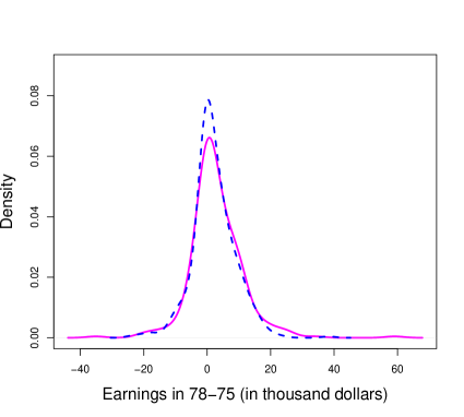
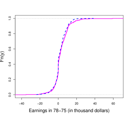
Figure 2: Unconditional empirical density function (left) and distribution function (right) of the difference of earnings from 1975 to 1978. The dashed line is associated with the control group and the solid line is associated with the treatment group.

$\tau$(%)	10	20	30	50	70	80	90
Treatment	-4.38	-1.55	0.00	1.40	5.48	8.50	11.15
Control	-4.91	-1.73	-0.17	0.74	4.44	7.16	10.56

Table 4: The unconditional sample quantiles of treatment and control groups.

Type of test	Statistics	$p$-value
Kolmogorov-Smirnov	0.0686	0.3835
Cramér-von Mises	0.2236	0.7739

Table 5: The two sample empirical cdf tests results for treatment and control groups.

Next we apply our test on quantile regression to evaluate the treatment effect. In order to compare with Delgado and Escanciano (2013), we first focus on the case of a one-dimensional covariate. The first covariate $X_{1i}$ is the age. The second covariate $X_{2i}$ is the number of years of schooling. The sample values of schooling years lie in the range of $[3,16]$ and age lies between $[17,55]$. In order to avoid boundary effect and sparsity of the samples, we look at the ranges [7,13] for schooling years and [19,31] for age. We apply the bootstrap CC method for quantiles $\tau=0.1,0.2,0.3,0.5,0.7,0.8$ and $0.9$. We apply the quartic kernel. The cross-validated bandwidths are chosen in the same way as for conditional densities with the R package np. The resulting bandwidths are (2.2691,2.5016) for the treatment group and (2.7204, 5.9408) for the control group. In particular, for smoothing the data of the treatment group, for $\tau=0.1$ and $0.9$, we enlarge the cross-validated bandwidths by a constant of $1.7$; for $\tau=0.2,0.3,0.7,0.8$, the cross-validated bandwidths are enlarged by constant factor $1.3$. These inflated bandwidths are used to handle violent roughness in extreme quantile levels. The bootstrap CCs are computed with 10,000 repetitions. The level of the test is $\alpha=5\%$.

The results of the two quantile regressions with one-dimensional covariate, and their CCs for various quantile levels are presented in Figure 3 and 4. We observe that for all chosen quantile levels the quantile estimates associated to the treatment group lie above that of the control group when age is over certain levels, and particularly for $\tau=10\%,50\%,80\%$ and $90\%$, the quantile estimates for treatment group exceeds the upper CCs for the quantile estimates of the control group. On the other hand, at $\tau=10\%$, the quantile estimates for the control group drop below the CC for treatment group for age greater than 27. Hence, the results here show a tendency that both the downside risk reduction and the upside potential enhancement of earnings growth are achieved, as the older individuals benefit the most from the treatment. Note that we observe a heterogeneous treatment effect in age and the weak dominance of the conditional quantiles of the treatment group with respect to those of the control group, i.e., (32) holds for the chosen quantile levels, which are in line with the findings of Delgado and Escanciano (2013).

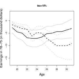
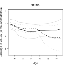
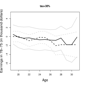
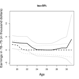
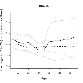
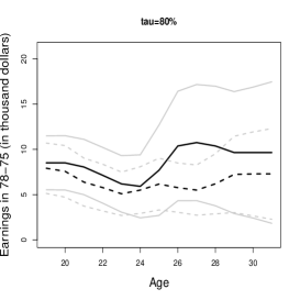
Figure 3: Nonparametric quantile regression estimates and CCs for the changes in earnings between 1975-1978 as a function of age. The solid dark lines correspond to the conditional quantile of the treatment group and the solid light lines sandwich its CC, and the dashed dark lines correspond to the conditional quantiles of the control group and the solid light lines sandwich its CC.

We now turn to Figure 4, where the covariate is the years of schooling. The treatment effect is not significant for conditional quantiles at levels $\tau=10\%,20\%$ and $30\%$. This suggests that the treatment does little to reduce the downside risk of the earnings growth for individuals with various degrees of education. Nonetheless, we constantly observe that the regression curves of the treatment group rise above that of the control group after a certain level of the years of schooling for quantile levels $\tau=50\%,70\%,80\%$ and $90\%$. Notice that for $\tau=50\%$ and $80\%$ the regression curves associated to the treatment group reach the upper boundary of the CC of the control group. This suggests that the treatment effect tends to raise the upside potential of the earnings growth, in particular for those individuals who spent more years in the school. It is worth noting that we also see a heterogeneous treatment effect in schooling years, although the heterogeneity in education is less strong than the heterogeneity in age.

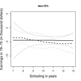
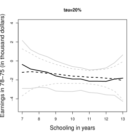
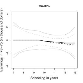
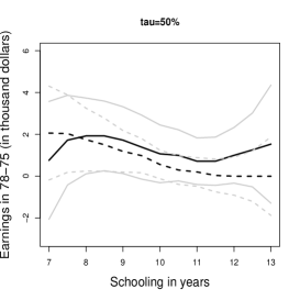
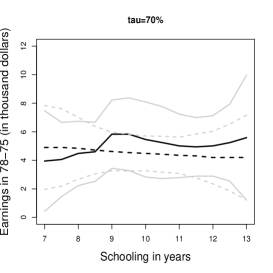
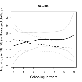
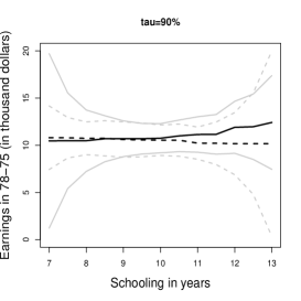
Figure 4: Nonparametric quantile regression estimates and CCs for the changes in earnings between 1975-1978 as a function of years of schooling. The solid dark lines correspond to the conditional quantile of the treatment group and the solid light lines sandwich its CC, and the dashed dark lines correspond to the conditional quantiles of the control group and the solid light lines sandwich its CC.

The previous regression analyses separately conditioning on covariates age and schooling years only give a limited view on the performance of the program, we now proceed to the analysis conditioning on the two covariates jointly $(X_{1i},X_{2i})$. The estimation settings are similar to the case of univariate covariate. Figure 5 shows the quantile regression CCs. From a first glance of the pictures, the $\tau$-quantile CC of the treatment group and that of the control group overlap extensively for all $\tau$. We could not find sufficient evidence to reject the null hypothesis that the conditional distribution of treatment group and control group are equivalent.

(a) $\tau=10\%$

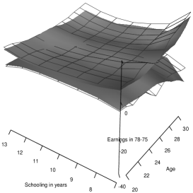
(b) $\tau=20\%$

(c) $\tau=30\%$

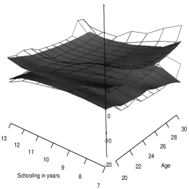
(d) $\tau=50\%$

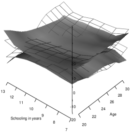
(e) $\tau=70\%$

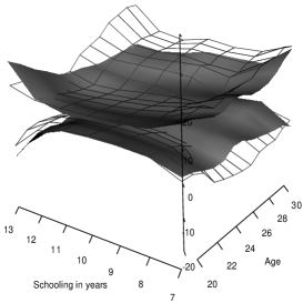
(f) $\tau=80\%$

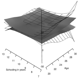
(g) $\tau=90\%$

Figure 5: The CCs for the treatment group and the control group. The net surface corresponds to the control group quantile CC and the solid surface corresponds to the treatment group quantile CC.

The second observation obtained from comparing subfigures in Figure 6, we find that the treatment has larger impact in raising the upper bound of the earnings growth than improving the lower bound. For lower quantile levels $\tau=10\%,20\%$ and 30% the solid surfaces uniformly lie inside the CC of the control group, while for $\tau=50\%,70\%,80\%$ and $90\%$, we see several positive exceedances over the upper boundary of the CC of the control group. Hence, the program tends to do better at raising the upper bound of the earnings growth but does worse at improving the lower bound of the earnings growth. In other words, the program tends to increase the potential for high earnings growth but does little in reducing the risk of negative earnings growth.

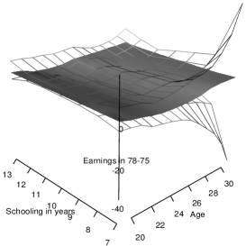
(a) $\tau=10\%$

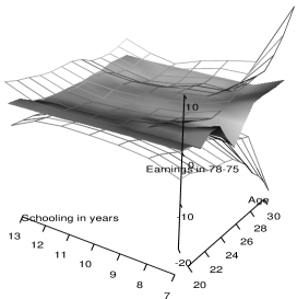
(b) $\tau=20\%$

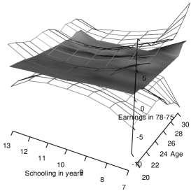
(c) $\tau=30\%$

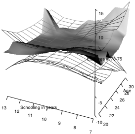
(d) $\tau=50\%$

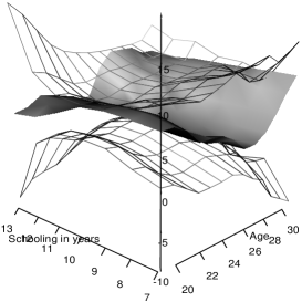
(e) $\tau=70\%$

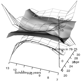
(f) $\tau=80\%$

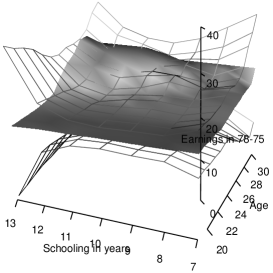
(g) $\tau=90\%$

Figure 6: The conditional quantiles (solid surfaces) for the treatment group and the CCs (net surfaces) for the control group.

Our last conclusion comes from inspecting the shape of the surfaces: conditioning on different levels of years of schooling (age), the treatment effect is heterogeneous in age (years of schooling). The most interesting cases occur when conditioning on high age and high years of schooling. Indeed, when considering the cases of $\tau=80\%$ and $90\%$, when conditioning on the years of schooling at 12 (corresponding to finishing the high school), the earnings increment of the treatment group rises above the upper boundary of the CC of the control group. This suggests that the individuals who are older and have more years of schooling tend to benefit more from the treatment.

Supplementary Materials

Section A contains the detailed proofs of Theorems 2.1, 2.3, 3.1 and Lemmas 2.6 and 3.2, as well as intermediate results. Section B contains some results obtained by other authors, which we use in our study. We incorporate them here for the sake of completeness.

Appendix A Assumptions

1. $K$ is of order $s-1$ (see (A3)) has bounded support $[-A,A]^{d}$ for $A>0$ a positive real scalar, is continuously differentiable up to order $d$ with bounded derivatives, i.e. $\partial^{\mbox{\scriptsize\boldmath$\alpha$}}K\in L^{1}(\mathbb{R}^{d})$ exists and is continuous for all multi-indices ${\mbox{\boldmath$\alpha$}}\in\{0,1\}^{d}$

2. Let $a_{n}$ be an increasing sequence, $a_{n}\rightarrow\infty$ as $n\rightarrow\infty,$ and the marginal density $f_{Y}$ be such that

   $$(\log n)h^{-3d}\int_{|y|>a_{n}}f_{Y}(y)dy=\mathcal{O}(1)$$ (33)

   and

   $$(\log n)h^{-d}\int_{|y|>a_{n}}f_{Y|{\mbox{\scriptsize\boldmath$X$}}}(y|{\mbox{\boldmath$x$}})dy=\mathcal{O}(1),\mbox{ for all }{\mbox{\boldmath$x$}}\in\mathcal{D}$$

   as $n\rightarrow\infty$ hold.

3. The function $\theta_{0}({\mbox{\boldmath$x$}})$ is continuously differentiable and is in Hölder class with order $s>d$.

4. $f_{\mbox{\scriptsize\boldmath$X$}}({\mbox{\boldmath$x$}})$ is bounded, continuously differentiable and its gradient is uniformly bounded. Moreover, $\inf_{{\mbox{\scriptsize\boldmath$x$}}\in\mathcal{D}}f_{\mbox{\scriptsize\boldmath$X$}}({\mbox{\boldmath$x$}})>0$.

5. The joint probability density function $f(y,{\mbox{\boldmath$u$}})$ is bounded, positive and continuously differentiable up to $s$th order (needed for Rosenblatt transform). The conditional density $f_{Y|{\mbox{\scriptsize\boldmath$X$}}}(y|{\mbox{\boldmath$x$}})$ exists and is boudned and continuouly differentiable with respect to $x$. Moreover, $\inf_{{\mbox{\scriptsize\boldmath$x$}}\in\mathcal{D}}f_{Y|{\mbox{\scriptsize\boldmath$X$}}}\big{(}\theta_{0}({\mbox{\boldmath$x$}})|{\mbox{\boldmath$x$}}\big{)}>0$.

6. $h$ satisfies $\sqrt{nh^{d}}h^{s}\sqrt{\log n}\rightarrow 0$ (undersmoothing), and $nh^{3d}(\log n)^{-2}\to\infty$.

• $\sup_{{\mbox{\scriptsize\boldmath$x$}}\in\mathcal{D}}\left|\int v^{b_{1}}f_{{\varepsilon}|{\mbox{\scriptsize\boldmath$X$}}}(v|{\mbox{\boldmath$x$}})dv\right|<\infty$, for some $b_{1}>0$.

1. $L$ is a Lipschitz, bounded, symmetric kernel. $G$ is Lipschitz continuous cdf, and $g$ is the derivative of $G$ and is also a density, which is Lipschitz continuous, bounded, symmetric and five times continuously differentiable kernel.

2. $F_{{\varepsilon}|{\mbox{\scriptsize\boldmath$X$}}}(v|{\mbox{\boldmath$x$}})$ is in $s^{\prime}+1$ order Hölder class with respect to $v$ and continuous in $x$, $s^{\prime}>\max\{2,d\}$. $f_{\mbox{\scriptsize\boldmath$X$}}({\mbox{\boldmath$x$}})$ is in second order Hölder class with respect to $x$ and $v$. $\mbox{\sf E}[\psi^{2}({\varepsilon}_{i})|{\mbox{\boldmath$x$}}]$ is second order continuously differentiable with respect to ${\mbox{\boldmath$x$}}\in\mathcal{D}$.

3. $nh_{0}\bar{h}^{d}\to\infty$, $h_{0},\bar{h}=\mathcal{O}(n^{-\nu})$, where $\nu>0$.

1. There exist an increasing sequence $c_{n}$, $c_{n}\rightarrow\infty$ as $n\rightarrow\infty$ such that

   $$(\log n)^{3}(nh^{6d})^{-1}\int_{|v|>c_{n}/2}f_{\varepsilon}(v)dv=\mathcal{O}(1),$$ (34)

   as $n\rightarrow\infty$.

2. $\sup_{{\mbox{\scriptsize\boldmath$x$}}\in\mathcal{D}}\left|\int v^{b}f_{{\varepsilon}|{\mbox{\scriptsize\boldmath$X$}}}(v|{\mbox{\boldmath$x$}})dv\right|<\infty$, for some $b>0$.

The assumptions (A1)-(A5) are assumptions frequently seen in the papers of confidence corridors, such as Härdle (1989), Härdle and Song (2010) and Guo and Härdle (2012). (EA2) and (EC1) essentially give the uniform bound on the 2nd order tail variation, which is crucial in the sequence of approximations for expectile regression. (B1)-(B3) are similar to the assumptions listed in chapter 6.1 of Li and Racine (2007). (A6) characterizes the two conflicting conditions: the undersmoothing of our estimator and the convergence of the strong approximation. To make the condition hold, sometimes we need large $s$ for high dimension, the smoothness of the true function. (C1) and (EC1) are relevant to the theory of bootstrap, where we need bounds on the tail probability and 2nd order variation.

References

- (1)
- Bickel and Rosenblatt (1973) Bickel, P. J. and Rosenblatt, M. (1973). On some global measures of the deviations of density function estimates, The Annals of Statistics 1(6): 1071–1095.
- Bissantz et al. (2007) Bissantz, N., Dümbgen, L., Holzmann, H. and Munk, A. (2007). Nonparametric confidence bands in deconvolution density estimation, Journal of the Royal Statistical Society: Series B 69(3): 483–506.
- Claeskens and Van Keilegom (2003) Claeskens, G. and Van Keilegom, I. (2003). Bootstrap confidence bands for regression curves and their derivatives, The Annals of Statistics 31(6): 1852–1884.
- Dehejia and Wahba (1999) Dehejia, R. H. and Wahba, S. (1999). Causal effects in nonexperimental studies: Reevaluating the evaluation of training programs, Journal of the American Statistical Association 94(448): 1053–1062.
- Delgado and Escanciano (2013) Delgado, M. A. and Escanciano, J. C. (2013). Conditional stochastic dominance testing, Journal of Business & Economic Statistics 31(1): 16–28.
- Doksum (1974) Doksum, K. (1974). Empirical probability plots and statistical inference for nonlinear models in the two-sample case, The Annals of Statistics 2(2): 267–277.
- Fan and Liu (2013) Fan, Y. and Liu, R. (2013). A direct approach to inference in nonparametric and semiparametric quantile regression models, Preprint.
- Feng et al. (2011) Feng, X., He, X. and Hu, J. (2011). Wild bootstrap for quantile regression, Biometrika 98(4): 995–999.
- Giné and Nickl (2010) Giné, E. and Nickl, R. (2010). Confidence bands in density estimation, The Annals of Statistics 38(2): 1122–1170.
- Guerre and Sabbah (2012) Guerre, E. and Sabbah, C. (2012). Uniform bias study and Bahadur representation for local polynomial estimators of the conditional quantile function, Econometric Theory 28(1): 87–129.
- Guo and Härdle (2012) Guo, M. and Härdle, W. (2012). Simultaneous confidence bands for expectile functions, AStA Advances in Statistical Analysis 96(4): 517–541.
- Hall (1979) Hall, P. (1979). On the rate of convergence of normal extremes, Journal of Applied Probability 16(2): 433–439.
- Hall (1991) Hall, P. (1991). On convergence rates of suprema, Probability Theory and Related Fields 89(4): 447–455.
- Hall (1992) Hall, P. (1992). Effect of bias estimation on coverage accuracy of bootstrap confidence intervals for a probability density, The Annals of Statistics 20(2): 675–694.
- Hall and Horowitz (2013) Hall, P. and Horowitz, J. (2013). A simple bootstrap method for constructing nonparametric confidence bands for functions, The Annals of Statistics 41(4): 1892–1921.
- Härdle (1989) Härdle, W. (1989). Asymptotic maximal deviation of -smoothers, Journal of Multivariate Analysis 29(2): 163–179.
- Härdle and Song (2010) Härdle, W. and Song, S. (2010). Confidence bands in quantile regression, Econometric Theory 26(4): 1180–1200.
- Johnston (1982) Johnston, G. J. (1982). Probabilities of maximal deviations for nonparametric regression function estimates, Journal of Multivariate Analysis 12(3): 402–414.
- Jones (1994) Jones, M. C. (1994). Expectiles and -quantiles are quantiles, Statistics & Probability Letters 20(2): 149–153.
- Kiwitt and Neumeyer (2012) Kiwitt, S. and Neumeyer, N. (2012). Estimating the conditional error distribution in non-parametric regression, Scandinavian Journal of Statistics 39(2): 259–281.
- Koenker (2005) Koenker, R. (2005). Quantile Regression, Econometric Society Monographs, Cambridge University Press, New York.
- Kong et al. (2010) Kong, E., Linton, O. and Xia, Y. (2010). Uniform Bahadur representation for local polynomial estimates of -regression and its application to the additive model, Econometric Theory 26(5): 1529–1564.
- LaLonde (1986) LaLonde, R. J. (1986). Evaluating the econometric evaluations of training programs with experimental data, The American Economic Review 76(4): 604–620.
- Lehmann (1975) Lehmann, E. L. (1975). Nonparametrics: Statistical Models Based on Ranks, Springer, San Francisco, CA.
- Li et al. (2013) Li, Q., Lin, J. and Racine, J. S. (2013). Optimal bandwidth selection for nonparametric conditional distribution and quantile functions, Journal of Business & Economic Statistics 31(1): 57–65.
- Li and Racine (2007) Li, Q. and Racine, J. S. (2007). Nonparametric Econometrics: Theory and Practice, Princeton university press, New Jersey.
- Lounici and Nickl (2011) Lounici, K. and Nickl, R. (2011). Global uniform risk bounds for wavelet deconvolution estimators, The Annals of Statistics 39(1): 201–231.
- Mammen et al. (2013) Mammen, E., Van Keilegom, I. and Yu, K. (2013). Expansion for moments of regression quantiles with applications to nonparametric testing, ArXiv e-prints .
- Mojirsheibani (2012) Mojirsheibani, M. (2012). A weighted bootstrap approximation of the maximal deviation of kernel density estimates over general compact sets, Journal of Multivariate Analysis 112: 230–241.
- Muhsal and Neumeyer (2010) Muhsal, B. and Neumeyer, N. (2010). A note on residual-based empirical likelihood kernel density estimator, Electronic Journal of Statistics 4: 1386–1401.
- Newey and Powell (1987) Newey, W. K. and Powell, J. L. (1987). Asymmetric least squares estimation and testing, Econometrica 55(4): 819–847.
- Proksch et al. (2014) Proksch, K., Bissantz, N. and Dette, H. (2014). Confidence bands for multivariate and time dependent inverse regression models, Bernoulli . To appear.
- Rosenblatt (1976) Rosenblatt, M. (1976). On the maximal deviation of -dimensional density estimates, The Annals of Probability 4(6): 1009–1015.
- Smirnov (1950) Smirnov, N. V. (1950). On the construction of confidence regions for the density of distribution of random variables, Doklady Akad. Nauk SSSR 74: 189–191.
- Song et al. (2012) Song, S., Ritov, Y. and Härdle, W. (2012). Partial linear quantile regression and bootstrap confidence bands, Journal of Multivariate Analysis 107: 244–262.
- Yu and Jones (1998) Yu, K. and Jones, M. C. (1998). Local linear quantile regression, Journal of the American Statistical Association 93(441): 228–237.