WENO schemes applied to the quasi-relativistic Vlasov–Maxwell model for laser-plasma interaction

Abstract

In this paper we focus on WENO-based methods for the simulation of the 1D Quasi-Relativistic Vlasov–Maxwell (QRVM) model used to describe how a laser wave interacts with and heats a plasma by penetrating into it. We propose several non-oscillatory methods based on either Runge–Kutta (explicit) or Time-Splitting (implicit) time discretizations. We then show preliminary numerical experiments.

Résumé Schémas WENO appliqués au modèle Vlasov–Maxwell quasi-relativiste pour l’interaction laser-plasma. Dans cet article, nous nous intéressons aux méthodes de type WENO pour la simulation du modèle Vlasov–Maxwell quasi-relativiste (QRVM) 1D, utilisé pour décrire la façon dont une onde laser interagit avec un plasma et le réchauffe en le pénétrant. Nous proposons plusieurs méthodes non oscillatoires fondées sur des discrétisations en temps soit Runge–Kutta (explicites) soit Time-Splitting (implicites). Ensuite, nous présentons des expériences numériques préliminaires.

, ,

1 Introduction

The object of our study is the dimensionless 1D quasi-relativistic Vlasov–Maxwell (QRVM) system:

$$\left\{\begin{array}[]{l}\displaystyle\frac{\partial f}{\partial t}+v(p)\frac{\partial f}{\partial x}+F{(t,x)}\frac{\partial f}{\partial p}=0\quad\mbox{(collisionless Vlasov)},\qquad F=-\left(E+AB\right)\\[11.38109pt] \displaystyle\frac{\partial E}{\partial x}=\eta^{-2}\left(\varrho_{\mathrm{ext}}-\varrho\right)\qquad\mbox{(Poisson equation)}\\[11.38109pt] \displaystyle\frac{\partial A}{\partial t}=-\mathcal{E},\qquad\frac{\partial\mathcal{E}}{\partial t}=\eta^{-2}A\varrho-\frac{\partial B}{\partial x},\qquad\frac{\partial B}{\partial t}=-\frac{\partial\mathcal{E}}{\partial x},\qquad\qquad\mbox{(Maxwell equations)}\\[11.38109pt] \displaystyle v(p)=\frac{p}{\sqrt{1+p^{2}}},\qquad\varrho=\int f\,\mathrm{d}p\qquad\mbox{(relativistic character)}\end{array}\right.$$ (1)

solved for $(t,x,p)\in[0,+\infty[\times[0,1]\times\mathbb{R}$, endowed with periodic boundary conditions in $x$. Problem (1) needs several initial conditions: one for the distribution function $f$; three for the magnetic potential $A$ and its derivatives, the magnetic field $B$ and the transverse electric field $\mathcal{E}$, which are related by

$$\mathcal{E}=-\frac{\partial A}{\partial t}\qquad\mbox{and}\qquad B=\frac{\partial A}{\partial x}.$$ (2)

The quantity $\varrho_{\text{ext}}$ represents the immobile ion background which keeps the plasma neutral. The interest in this Vlasov–Maxwell system is motivated by its importance in plasma physics: it describes laser-plasma interaction, i.e. the action of a laser wave, called pump, penetrating into a plasma and heating it, while interacting with electrostatic waves and accelerating the electrons. This model, and its variants, have been long known in the plasma physics community [1, 2, and references therein]. Its derivation and a discussion about the global existence and uniqueness of classical solutions can be found in [3].

In order to solve (1) numerically, one has to choose a time discretization method, a Vlasov solver and a Maxwell solver. So far, characteristic solvers have been generally used for the Maxwell part, combined with various semi-Lagrangian methods [1, 2, 4] for Vlasov, as well as wavelets [5]. Time-splitting methods were often used for the quasi-relativistic model, though they are unstable with a fully relativistic model [2].

The goal of this article is to introduce several Weighted Essentially Non-Oscillatory (WENO) schemes for the QRVM model, and to perform preliminary tests and comparisons, in order to decide which schemes are more suitable. In Table 1 we summarize all the combinations we have considered and tested.

time integration	RK	TS
Vlasov equation	FDWENO	DSLWENO
		CSLWENO
Maxwell equations	RK	RK
	LF	LF

Table 1: The overall integration strategy. The schemes in italic are implicit.

RK refers to the Total-Variation-Diminishing Runge–Kutta scheme [6].
TS refers to the Time-Splitting (Strang) scheme [7, 8].
FDWENO stands for the Finite-Difference Weighted Essentially Non Oscillatory interpolator for the approximation of partial derivatives [6].
DSLWENO stands for the non-conservative Direct Semi-Lagrangian scheme [8], coupled to the Point-Value WENO interpolator [9, 10, 8].
CSLWENO stands for the Conservative Semi-Lagrangian scheme, based on the Flux-Balance-Method (FBM) [11], coupled to the FBMWENO described later on.
LF stands for Leap-Frog scheme (aka Yee scheme).

For the sake of clarity, we shall make use of a three-word notation to describe the coupling: {time discretization}-{Vlasov solver}-{Maxwell solver}, e.g., TS-DSLWENO-LF.

The outline of this paper is the following: in Section 2 we describe the initial and boundary conditions and the discretization of the system; in Section 3 we describe the time-integration strategy; in Section 4 we show numerical experiments; and we conclude in Section 5.

2 Initial and boundary conditions, and discretization

2.1 Initialization

Problem (1) needs two initializations: one for the distribution function $f(t,x,p)$, and one for the electro-magnetic variables $A(t,x)$, $B(t,x)$ and $\mathcal{E}(t,x)$.

2.1.1 Initialization of the distribution function

We suppose that a proportion $1-\alpha$ of the electrons are thermalized at a (dimensionless) cold velocity $v_{\mathrm{cold}}$, while the remaining proportion $\alpha$ are hot with (dimensionless) velocity $v_{\mathrm{hot}}$

$$G(p)=(1-\alpha)\,G_{\mathrm{cold}}(p)+\alpha\,G_{\mathrm{hot}}(p),$$

where we have split the Maxwellian $G(p)$ into a cold part $G_{\mathrm{cold}}(p)$, described by a classical Gaussian, and a hot part $G_{\mathrm{hot}}(p)$, described by a Jüttner distribution:

$$\underbrace{G_{\mathrm{cold}}(p)=\frac{\exp\left(-\frac{p^{2}}{2\,v_{\mathrm{cold}}^{2}}\right)}{\sqrt{2\pi}\,v_{\mathrm{cold}}}}_{\mbox{normalized classical Gaussian}}\qquad\mbox{and}\qquad\underbrace{G_{\mathrm{hot}}(p)=\frac{\exp\left(-\frac{\sqrt{1+p^{2}}-1}{v_{\mathrm{hot}}^{2}}\right)}{\mathop{{\int}}_{\!\!\!\mathbb{R}}\exp\left(-\frac{\sqrt{1+p^{2}}-1}{v_{\mathrm{hot}}^{2}}\right)\,\mathrm{d}p}}_{\mbox{normalized J\"{u}ttner distribution}}.$$

We shall introduce a fluctuation for the initial density

$$\varrho(0,x)=1+\frac{\varepsilon\,v_{\mathrm{cold}}\left(0.6\,k_{\mathrm{pla}}\right)}{\sqrt{1+3\,v_{\mathrm{cold}}^{2}\left(0.6\,k_{\mathrm{pla}}\right)^{2}}}\cos\left(2\pi\,k_{\mathrm{pla}}\,x\right),$$

for some spatial frequency $k_{\text{pla}}$. Consequently, a fluctuation is also introduced for the Maxwellian, hence, all in all, the initial distribution function reads

$$f(0,x,p)=\varrho(0,x)\cdot G(p-\varepsilon\,v_{\mathrm{cold}}\cos\left(2\pi\,k_{\mathrm{pla}}\,x\right)).$$

2.1.2 Initialization of the electro-magnetic field

The initial conditions for $A$, $B$ and $\mathcal{E}$ describe the pump wave which is going to interact with the plasma wave due to the density fluctuations.

Depending on the coupling we choose between the Vlasov and the Maxwell solvers, we shall need to set $A$, $B$ and $\mathcal{E}$ at different initial times and positions, which is why we keep the maximum generality by writing them as $(t,x)$-dependent:

$$A\left(t,x\right) =A_{0}\sin\left(2\pi\,k_{\mathrm{pump}}\,x-\omega_{0}\,t\right),\qquad B\left(t,x\right)=2\pi\,A_{0}\,k_{\mathrm{pump}}\cos\left(2\pi\,k_{\mathrm{pump}}\,x-\omega_{0}\,t\right),$$

$$\mathcal{E}\left(t,x\right) =A_{0}\,\omega_{0}\cos\left(2\pi\,k_{\mathrm{pump}}\,x-\omega_{0}\,t\right).$$

One checks that the relation between $A$, $B$ and $\mathcal{E}$ at any chosen initial time is given by (2).

2.1.3 Boundary conditions

Problem (1) is endowed with periodic boundary conditions in the $x$-dimension. To keep the computational domain bounded and enforce mass conservation, we use Neumann boundary conditions in the $p$-dimension. Actually, if the size of the domain is properly chosen, no electrons should reach the $p$-border. The boundary conditions are implemented as:

$$f_{-i,j} =f_{i+N_{x},j} \mbox{for }i=1,\dots,N_{\mathrm{ghp}},\quad j=1,\dots,N_{p}-1$$

$$f_{N_{x}+i,j} =f_{i,j} \mbox{for }i=1,\dots,N_{\mathrm{ghp}},\quad j=1,\dots,N_{p}-1$$

$$f_{i,N_{p}+j} =f_{i,N_{p}-1} \mbox{for }i=0,\dots,N_{x},\quad j=0,\dots,N_{\mathrm{ghp}}$$

$$f_{i,-j} =f_{i,1} \mbox{for }i=0,\dots,N_{x},\quad j=0,\dots,N_{\mathrm{ghp}}.$$

2.2 Discretization

We mesh the computational domain $\displaystyle\Omega=[0,1]\times\left[-p_{\max},p_{\max}\right]$ by uniform grids:

$$\left(x_{i},p_{j}\right)=\left(i\,\Delta x,j\,\Delta p\right),\qquad\!\!\!\!\left(\Delta x,\Delta p\right)=\left(\dfrac{1}{N_{x}},\dfrac{2\,p_{\max}}{N_{p}}\right).$$

In order to take into account the boundary conditions, ghost points outside the physical domain are used.

3 Time integration

In this section, we take care of the time integration for the Vlasov equation

$$\frac{\partial f}{\partial t}+v(p)\frac{\partial f}{\partial x}+F(t,x)\frac{\partial f}{\partial p}=0,\qquad F=-\left(E+A\,B\right)$$ (3)

and for the set of Maxwell equations

$$\frac{\partial A}{\partial t}=-\mathcal{E},\qquad\frac{\partial\mathcal{E}}{\partial t}=\eta^{-2}A\varrho-\frac{\partial B}{\partial x},\qquad\frac{\partial B}{\partial t}=-\frac{\partial\mathcal{E}}{\partial x}.$$ (4)

As for the Poisson equation

$$\frac{\partial E}{\partial x}=\eta^{-2}\left(\varrho_{\mathrm{ext}}-\varrho\right),$$

we use the fast, spectrally-accurate solver, whose details can be found in [12].

We wish to test two different integration strategies, which are summarized in Table 1.

TS is implicit in the sense that it generally uses implicit schemes for advection, thus weakening the constraints on the time step; on the other hand, RK is explicit, thus it requires a CFL condition.

This section is organized as follows: in Section 3.1 we introduce the Runge–Kutta based schemes; in Section 3.2 we introduce the Strang-splitting based schemes; in Section 3.3 we introduce leap-frog and multi-stage schemes to integrate (4); in Section 3.4 we summarize all the resulting schemes.

3.1 RK-FDWENO scheme

The explicit third-order TVD Runge–Kutta strategy consists in integrating, from time $t^{n}$ to $t^{n+1}$, the Vlasov equation

$$\frac{\partial f}{\partial t}=-v(p)\frac{\partial f}{\partial x}-F(t,x)\frac{\partial f}{\partial p}=:\mathcal{H}\left[t,f\right]$$

as

$$f^{n,1} =f^{n}+\Delta t\,\mathcal{H}\left[t^{n},f^{n}\right],\quad f^{n,2}=\frac{3}{4}f^{n}+\frac{1}{4}f^{n,1}+\frac{1}{4}\Delta t\,\mathcal{H}\left[t^{n}+\Delta t,f^{n,1}\right],$$

$$f^{n+1} =\frac{1}{3}f^{n}+\frac{2}{3}f^{n,2}+\frac{2}{3}\Delta t\,\mathcal{H}\left[t^{n}+\frac{\Delta t}{2},f^{n,2}\right].$$ (5)

The partial derivatives are approximated through the fifth-order FDWENO routine for finite differences, whose details can be found, for instance, in [13, 14] and references therein. As this scheme is quite classical, we believe it does not deserve further details here. The scheme is subject to a CFL constraint for stability:

$$\Delta t<\dfrac{1}{\dfrac{\left\|v(p)\right\|_{\infty}}{\Delta x}+\dfrac{\left\|F\right\|_{\infty}}{\Delta p}}.$$

Remark that we have to use the correct upwinding and that, with proper boundary conditions (see Section 2.1.3), the scheme enforces mass conservation.

RK requires the calculation of the Lorentz force at three different times

$$F\left(t^{n}\right)=:F^{n},\quad F\left(t^{n}+\Delta t\right)=:F^{n+1},\quad F\left(t^{n}+\frac{1}{2}\Delta t\right)=:F^{n+1/2}.$$

Computing the electrostatic field $E(t)$ at the desired times is easy, because it is consistent with the distribution function $f(t)$; conversely, obtaining the magnetic variables $A(t)$ and $B(t)$ is slightly more complicated, because they follow their own evolution equations. In case the time integrator for the Maxwell equations does not provide us with $A$ and $B$ at the desired times, we can estimate them by interpolations.

3.2 TS-DSLWENO and TS-CSLWENO schemes

The (Strang) Time-Splitting strategy [7, 15] approximates the integration of the Vlasov equation

$$\frac{\partial f}{\partial t}+v(p)\frac{\partial f}{\partial x}+F{(t,x)}\frac{\partial f}{\partial p}=0$$

as a combination of partial solutions along the $x$-dimension and the $p$-dimension:

$$\frac{\partial f}{\partial t}+v(p)\frac{\partial f}{\partial x}=0\qquad\mbox{and}\qquad\frac{\partial f}{\partial t}+F{(t,x)}\frac{\partial f}{\partial p}=0.$$ (6)

We advect $f^{n}\longmapsto f^{n+1}$ by means of the advection field evaluated at time $t^{n+1/2}$, a strategy called prediction/correction [16, 17], summarized on Figure 1, which gives a scheme of order 2 in time as soon as $F(t^{n+1/2})$ is approximated at order 1.

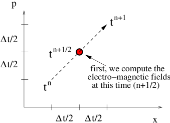
(a) Prediction.

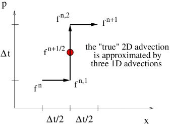
(b) Correction.

Figure 1: Prediction/correction strategy.

In principle, the one-dimensional PDEs (6) can be solved by means of any time integrator; here we propose a direct semi-Lagrangian (DSL) strategy (non-conservative), fully described in [12], and a conservative semi-Lagrangian (CSL) strategy, described in Section 3.2.1; semi-Lagrangian means that the method is characteristics-based.

3.2.1 CSL integration for 1D advection problems

The model equation which we solve is

$$\frac{\partial u}{\partial t}+\frac{\partial}{\partial x}\left[a(t,x)\,u\right]=0,\qquad u(t^{\star},x)=u^{\star}(x),\qquad(t,x)\in[0,+\infty[\times I$$

(being $a:[0,+\infty[\times I\to\mathbb{R}$ and $I\subseteq\mathbb{R}$ an interval) by means of a semi-Lagrangian conservative method; this strategy is taken from [11]. To this end, we evolve approximated cell averages

$$u^{n+1}_{i}\approx{\frac{1}{\Delta x}\int_{x_{i-1/2}}^{x_{i+1/2}}}u\left(t^{n+1},\xi\right)\,\mathrm{d}\xi$$

and use a semi-Lagrangian strategy by following the characteristics backward, along which $J\,u$ is conserved,

$$\int_{x_{i-1/2}}^{x_{i+1/2}}u\left(t^{n+1},\xi\right)\,\mathrm{d}\xi=\int_{x_{i-1/2}}^{x_{i+1/2}}u\left(t^{n},\mathcal{X}\left(t^{n};t^{n+1},\xi\right)\right)\,J\left(t^{n};t^{n+1},\xi\right)\,\mathrm{d}\xi,$$ (7)

with $\mathcal{X}(s;t,x)$ the characteristic and $J(s;t,x)$ its Jacobian:

$$\frac{\mathrm{d}\mathcal{X}(s;t,x)}{\mathrm{d}s}=a\left(s,\mathcal{X}(s;t,x)\right),\qquad\mathcal{X}(t;t,x)=x,\qquad J(s;t,x):=\det\dfrac{\partial\mathcal{X}(s;t,x)}{\partial x}.$$

If we change variables $\displaystyle\eta=\mathcal{X}\left(t^{n};t^{n+1},\xi\right)$ into (7), we get:

$${\frac{1}{\Delta x}\int_{x_{i-1/2}}^{x_{i+1/2}}}u\left(t^{n+1},\xi\right)\,\mathrm{d}\xi=\frac{1}{\Delta x}\int_{x^{\mathrm{back}}_{i-1/2}}^{x^{\mathrm{back}}_{i+1/2}}u\left(t^{n},\eta\right)\,\mathrm{d}\eta=\frac{U^{n}\left(x^{\mathrm{back}}_{i+1/2}\right)-U^{n}\left(x^{\mathrm{back}}_{i-1/2}\right)}{\Delta x},$$ (8)

where we have set $\displaystyle x^{\mathrm{back}}:=\mathcal{X}\left(t^{n};t^{n+1},x\right)$ and $U^{n}$ is a primitive of $u(t^{n},\cdot)$. This gives the following scheme:

$$u_{i}^{n+1}=\frac{\widetilde{U}^{n}\left(x^{\mathrm{back}}_{i+1/2}\right)-\widetilde{U}^{n}\left(x^{\mathrm{back}}_{i-1/2}\right)}{\Delta x},$$ (9)

where $\widetilde{U}^{n}$ is an approximation of $U^{n}$ based on values of $\left(u_{j}^{n}\right)_{j}$. The scheme is conservative if $u$ is compactly supported or under periodic boundary conditions. In our application, the computations are simplified by $a$ being a real constant. Therefore, we have explicit characteristics $\mathcal{X}(s;t,x)=x+a(s-t)$, so

$$u^{n+1}_{i}=\frac{\widetilde{U}^{n}\left(x_{i+1/2}-a\,\Delta t\right)-\widetilde{U}^{n}\left(x_{i-1/2}-a\,\Delta t\right)}{\Delta x}.$$

3.2.2 The WENO reconstruction for CSL (called FBMWENO)

In order to set up the scheme (9) we need an interpolator for the primitive $U$ (dropping the time-dependency notation from now on). In the WENO fashion, we shall perform a convex combination of several Lagrange polynomials interpolating $U$ at different substencils. We can adjust two parameters in order to obtain all the possible combinations: the degree $r_{\mathrm{tot}}$ of the Lagrange polynomial interpolating $U(x)$ in the whole stencil $\mathcal{S}$ (which thus contains $r_{\mathrm{tot}}+1$ points), and the degree $r_{\mathrm{sub}}$ of the Lagrange polynomials in the substencils (each substencil contains $r_{\mathrm{sub}}+1$ points). Let us also introduce the number of substencils $N_{\mathrm{sub}}:=r_{\mathrm{tot}}-r_{\mathrm{sub}}+1$.

Let us denote $P_{\nu}^{r}(x)$ the Lagrange polynomial interpolating the point values of the primitive $U$ at points $\left\{x_{\nu-r},\dots,x_{\nu}\right\}$. If $\displaystyle\mathcal{S}=\left\{x_{\mathrm{left}},\dots,x_{\mathrm{left}+r_{\mathrm{tot}}}=:x_{\mathrm{right}}\right\}$ is the big stencil used to approximate $U(x)$, then

$$U(x)\approx\widetilde{U}(x):=\sum_{\ell=0}^{N_{\mathrm{sub}}-1}\omega_{\ell}(x)\,P^{r_{\mathrm{sub}}}_{\mathrm{right}-\ell}(x).$$

In order to define the weights

$$\omega_{\ell}(x):=\frac{\tilde{\omega}_{\ell}(x)}{\sum_{\ell^{\prime}=0}^{N_{\mathrm{sub}}-1}\tilde{\omega}_{\ell^{\prime}}(x)},\qquad\tilde{\omega}_{\ell}(x):=\frac{C_{\ell}(x)}{\left(10^{-6}+\sigma_{\ell}\right)^{2}},\qquad\ell=0,\dots,N_{\mathrm{sub}}-1$$

we need two ingredients: the polynomials $\left\{C_{\ell}(x)\right\}_{\ell=0}^{N_{\mathrm{sub}}-1}$ defined by the relation

$$P_{\mathrm{right}}^{r_{\mathrm{tot}}}(x)=\sum_{\ell=0}^{N_{\mathrm{sub}}-1}C_{\ell}(x)\,P_{\mathrm{right}-\ell}^{r_{\mathrm{sub}}}(x),$$

and the smoothness indicators $\left\{\sigma_{\ell}\right\}_{\ell=0}^{N_{\mathrm{sub}}-1}$, which we wish to define in such a way that the $u^{n+1}_{i}$ given by (9) is not polluted by spurious oscillations. To this end, we are not interested in the smoothness of $U$, rather in the smoothness of $u$.

Now, the derivative of $P^{r}_{\nu}(x)$ is a lower-order approximation to $u(x)$:

$$\mathcal{P}^{r}_{\nu}(x):=\frac{\mathrm{d}P^{r}_{\nu}}{\mathrm{d}x}(x)\approx u(x),$$

in the sense that if $P^{r}_{\nu}(x)$ approximates $U(x)$ at order $r+1$, $\mathcal{P}^{r}_{\nu}(x)$ approximates $u(x)$ at order $r$. We now fix the interval $I:=\left[x_{i-1/2},x_{i+1/2}\right]$ that contains the evaluation point and define the smoothness measurement as in the Jiang–Shu fashion [18]: for $\ell=0,\dots,N_{\mathrm{sub}}-1$

$$\sigma_{\ell}:=\sum_{k=1}^{r_{\mathrm{sub}}-1}\Delta x^{2k-1}\int_{I}\left[\left(\mathcal{P}_{\mathrm{right}-\ell}^{r_{\mathrm{sub}}}\right)^{(k)}(\xi)\right]^{2}\,\mathrm{d}\xi.$$

The polynomials $C_{\ell}(x)$ and constants $\sigma_{\ell}$ for $\left(r_{\mathrm{tot}},r_{\mathrm{sub}}\right)=(5,3)$ are given in Appendix B.

3.3 Integration of the Maxwell equations

We test two strategies: a leap-frog-type Yee scheme and a Runge–Kutta scheme. The Yee scheme will be coupled to both schemes for the Vlasov equation and the Runge–Kutta scheme will only be coupled to the Runge–Kutta scheme for the Vlasov equation.

In any case, once we have updated the ponderomotive force $\displaystyle\mathcal{F}=A\,B$ up to time $t^{n}$, we impose it has numerically zero average:

$$\bar{\mathcal{F}}^{n}:=\frac{1}{N_{x}}\sum_{i=0}^{N_{x}-1}\mathcal{F}^{n}_{i},\qquad\mbox{then}\qquad\mathcal{F}^{n}_{i}\longmapsto\mathcal{F}^{n}_{i}-\bar{\mathcal{F}}^{n}.$$

The LF scheme that we use for the Maxwell equations is second-order accurate in both space and time, and is known as the Yee scheme. It is of the leap-frog type with half-shifted variables: see Figure 2 for a sketch.

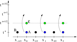
(a) leap $A^{n}_{i}\mapsto A^{n+1}_{i}$

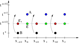
(b) leap $B^{n}_{i+1/2}\mapsto B^{n+1}_{i+1/2}$

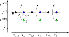
(c) leap $\mathcal{E}^{n+1/2}_{i}\mapsto\mathcal{E}^{n+3/2}_{i}$

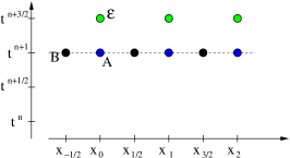
(d) at time $t^{n+1}$

Figure 2: Leap-frog strategy. The scheme is second-order in both time and space, because all the $t$- and $x$-derivatives are approximated by centered differences. Inside the figure $\displaystyle\mathcal{E}_{x}:=\frac{\partial\mathcal{E}}{\partial x}$ and $\displaystyle B_{x}:=\frac{\partial B}{\partial x}$.

Knowing $\varrho^{n+1}$, we advance in time $\left(A^{n},B^{n},\mathcal{E}^{n+1/2}\right)\longmapsto\left(A^{n+1},B^{n+1},\mathcal{E}^{n+3/2}\right)$ by centered finite differences:

• The evolution of the vector potential $A$ (Figure 2(a))

  $$\frac{\partial A}{\partial t}=-\mathcal{E}\qquad\mbox{gives}\qquad A^{n+1}_{i}=A^{n}_{i}-\mathcal{E}^{n+1/2}_{i}\Delta t.$$

• The evolution of the magnetic field $B$ (Figure 2(b)),

  $$\frac{\partial B}{\partial t}=-\frac{\partial\mathcal{E}}{\partial x}\qquad\mbox{gives}\qquad B^{n+1}_{i+1/2}=B^{n}_{i+1/2}-\frac{\Delta t}{\Delta x}\left(\mathcal{E}^{n+1/2}_{i+1}-\mathcal{E}^{n+1/2}_{i}\right).$$

• The evolution of the transverse electric field $\mathcal{E}$ (Figure 2(c)),

  $$\frac{\partial\mathcal{E}}{\partial t}=\eta^{-2}A\,\varrho-\frac{\partial B}{\partial x}\quad\mbox{gives}\quad\mathcal{E}^{n+3/2}_{i}=\mathcal{E}^{n+1/2}_{i}+\eta^{-2}A^{n+1}_{i}\varrho^{n+1}_{i}\Delta t-\frac{\Delta t}{\Delta x}\left(B^{n+1}_{i+1/2}-B^{n+1}_{i-1/2}\right).$$

3.4 Summary of the schemes

In order to construct the schemes resulting from the different choices for the time integrators of the Vlasov and the Maxwell equations (see Table 1), we have to be particularly careful in order to fit each block properly within the coupling.

3.4.1 TS-DSLWENO-LF and TS-CSLWENO-LF schemes

The scheme to advance

$$\left(f^{n},A^{n-1/2},B^{n-1/2},\mathcal{E}^{n}\right)\longmapsto\left(f^{n+1},A^{n+1/2},B^{n+1/2},\mathcal{E}^{n+1}\right)$$

is sketched on Figure 3. Notice that the time indices of $A,\ B,\ \mathcal{E}$ have been shifted by one half w.r.t. Section 3.3, so as to have the force at hand at time $t^{n+1/2}$, as explained in Section 3.2. Thus, $\varrho$ and $E$ must be available at $t^{n+1/2}$. This is done by computing them after the first half-advection in $x$ [15], see Figure 1(b). The difference between the two schemes is how the steps in Figure 3(a) and Figure 3(c) are performed, with a non-conservative method for DSLWENO and with a conservative one for CSLWENO.

(a) Strang 1/3

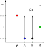
(b) leap-frog

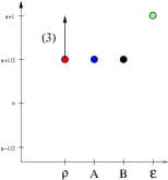
(c) Strang 2/3, 3/3

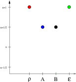
(d) at time $t^{n+1}$

Figure 3: TS-DSLWENO-LF and TS-CSLWENO-LF schemes. The schemes differ in how the Strang stages are performed.

3.4.2 RK-FDWENO-RK scheme

This scheme is obtained by applying the third-order TVD Runge–Kutta ODE solver (5) to a discretization in $x$ and $p$ of the Vlasov–Maxwell equations

$$\frac{\partial}{\partial t}\left(\begin{array}[]{c}f\\ \hdashline A\\ B\\ \mathcal{E}\end{array}\right)=\left(\begin{array}[]{c}-v(p)\frac{\partial f}{\partial x}-(E+A\,B)(t,x)\frac{\partial f}{\partial p}\\ \hdashline-\mathcal{E}\\ -\frac{\partial\mathcal{E}}{\partial x}\\ \eta^{-2}A\,\varrho-\frac{\partial B}{\partial x}\end{array}\right)=:\mathcal{H}\left[t,\left(\begin{array}[]{c}f\\ \hdashline A\\ B\\ \mathcal{E}\end{array}\right)\right],$$

where, as mentioned in Section 3.1, the $x$ and $p$ derivatives in the Vlasov equation are discretized by WENO finite differences, the $x$ derivatives in the Maxwell equations are discretized by linear finite differences; $\varrho$ is discretized by the midpoint quadrature rule, and $E$ is computed by the Poisson solver.

3.4.3 RK-FDWENO-LF scheme

The resulting scheme is depicted in Figure 4. Remark that the Yee scheme forces the time step $\Delta t$ to be kept fixed, despite the adaptive character of the Runge–Kutta scheme.

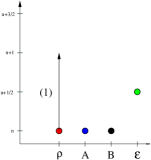
(a) RK 1/3

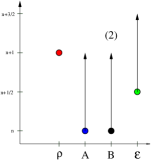
(b) leap-frog

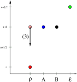
(c) RK 2/3

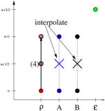
(d) RK 3/3

Figure 4: RK-FDWENO-LF scheme. This scheme is second-order in time (because of the interpolation and the first-order approximation of $\varrho$ used to evolve $\mathcal{E}$) and second-order in space.

4 Results for the quasi-relativistic Vlasov–Maxwell system

No WENO-based scheme has yet been extensively tested on the QRVM problem. Therefore, our first task is to decide which among the overall integration strategies introduced in Table 1 are suitable.

4.1 Empirical stability results

All the schemes proposed in this article seem stable from empirical observation, but RK-FDWENO-LF requires extremely small time steps in order not to blow up. A summary is given in Table 2.

Vlasov $\downarrow$                               Maxwell $\rightarrow$	LF	RK
RK-FDWENO-	☹	☺
TS-DSLWENO-	☹	not couplable
TS-CSLWENO-	☺	not couplable

Table 2: Quality of the results.

The evolution equations for $B$ and $\mathcal{E}$ can be rewritten as

$$\frac{\partial\left(B\pm\mathcal{E}\right)}{\partial t}\pm\frac{\partial\left(B\pm\mathcal{E}\right)}{\partial x}=\pm\eta^{-2}\,A\,\varrho,$$

therefore the condition

$$\Delta t<\Delta x$$ (10)

seems reasonable as constraint for stability of an explicit scheme.

If we take as reference a $400\times 400$ mesh, $\Delta x$ would be equal to $0.0025$. Notwithstanding, experiments suggest the threshold $\Delta t$ should be of order $10^{-5}$ for RK-FDWENO-LF. In the other cases, the RK-FDWENO-RK scheme, the TS-DSLWENO-LF scheme and the TS-CSLWENO-LF scheme, if the CFL parameter or the $\Delta t$ are adapted so as to fulfill (10), the simulations appear stable.

4.2 Quality of the results

On Figure 5 we compare at similar stages the evolution computed by the three most stable schemes. The dynamic of laser-plasma interaction [1, 2, 5] is precisely captured. The plasma wave, initiated by the initial fluctuations of the electron density, exchanges energy with the electrons and with the transverse electromagnetic wave. Vortices appear in phase space, due to the particles getting trapped by the plasma wave’s potential well and bouncing on its separatrices. The vortices show an oscillating behavior: they periodically inflate and deflate. One observes the well-known “filamentation” phenomenon: thin structures appear, then they are stretched thinner and folded, again and again.

We see that in the short term both the RK-based and the TS-based schemes behave well, but TS-CSLWENO-LF diffuses the microscopic details more than RK-FDWENO-RK, as the long-time behavior ($t=300$) shows.

On Figure 6 we plot the conservation properties: the relative variation (w.r.t. time $t=0$) of the mass, of the $L^{2}$-norm and of the total energy

$$W(t)=\overbrace{\underbrace{\frac{1}{2}\int_{0}^{1}A^{2}\varrho\,\mathrm{d}x}_{\mathrm{WTK}(t):=\mathrm{kinetic}}+\underbrace{\frac{\eta^{2}}{2}\int_{0}^{1}\left[\mathcal{E}^{2}+B^{2}\right]\mathrm{d}x}_{\mathrm{WTP}(t):=\mathrm{potential}}}^{\mathrm{WT}(t):=\mathrm{transversal}}+\overbrace{\underbrace{\int_{0}^{1}\int_{\mathbb{R}}\left(\sqrt{1+p^{2}}-1\right)f\,\mathrm{d}p\,\mathrm{d}x}_{\mathrm{WLK}(t):=\mathrm{kinetic}}+\underbrace{\frac{\eta^{2}}{2}\int_{0}^{1}E^{2}\,\mathrm{d}x}_{\mathrm{WLP}(t):=\mathrm{potential}}}^{\mathrm{WL}(t):=\mathrm{longitudinal}},$$ (11)

which is shown in [3] to be conserved by the system. We observe that around time 300 TS-DSLWENO-LF has gained about 13 % w.r.t. the normalized mass, which means that the plasma is strongly non-neutral, hence even the integration of the Poisson equation becomes meaningless because the periodicity is lost. RK-FDWENO-RK conserves better the $L^{2}$-norm, i.e. the microscopic details inside the computational domain, and the total energy.

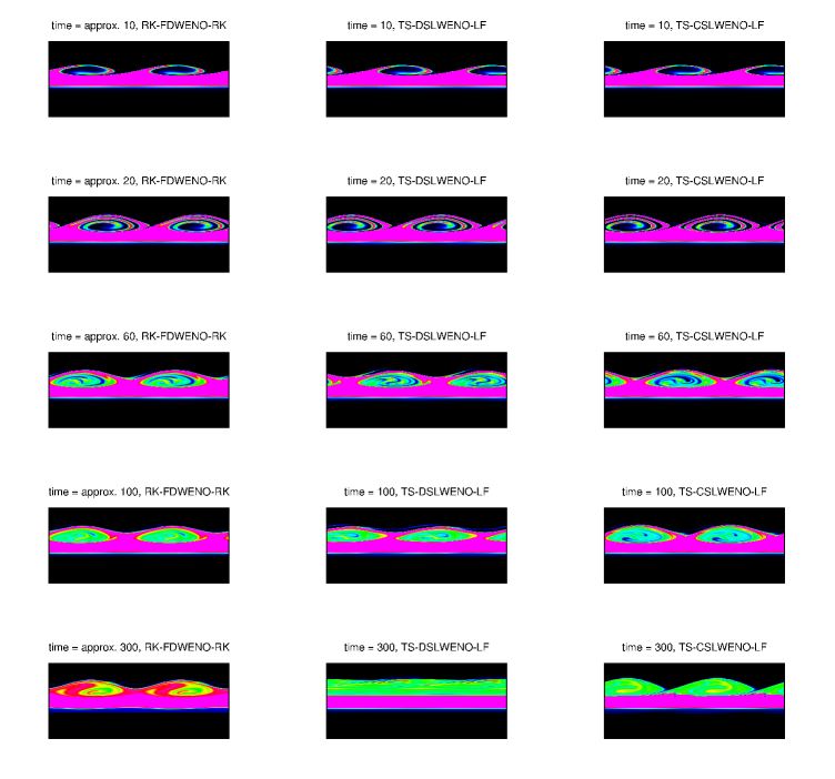
Figure 5: Comparison. Evolution of the system up to time $\approx 300$, for a $400\times 400$ mesh, using three different schemes. Left column: the explicit conservative RK-FDWENO-RK. Central column: the implicit non-conservative TS-DSLWENO-LF. Right column: the implicit conservative TS-CSLWENO-LF.

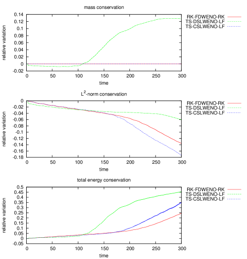
Figure 6: Conservation properties. Top: the relative variation of total mass w.r.t. the initial condition. Center: the relative variation of the $L^{2}$-norm w.r.t. the initial condition. Bottom: the relative variation of the total energy (11) w.r.t. the initial condition.

5 Conclusion

We have performed some preliminary tests of several WENO-based schemes to simulate the 1D quasi-relativistic Vlasov–Maxwell system, which models laser-plasma interaction. WENO schemes, with their high accuracy and robustness to the steep gradients created by filamentation, are ideally suited to capture the dynamic of this interaction. Indeed, our test cases have reproduced the qualitative behavior known from the literature since [1].

To decide which schemes are more suitable for the simulation of the QRVM problem, we tested the various combinations of Table 1. Some of them immediately appear unsatisfactory, either because they require ridiculously small time steps, or because they are strongly non-conservative. The two strategies which show the best behavior are RK-FDWENO-RK and TS-CSLWENO-LF, which are both conservative; the advantage of TS-CSLWENO-LF is its implicit character and weaker constraints on the time step, while its drawback is that in the long time it shows a more diffusive behavior.

From the computational point of view, WENO-based schemes have several other advantages. They are easily parallelizable: see for instance [19] for a parallel version of RK-FDWENO. They can be made adaptive relatively easily: see [12] for an AMR version of TS-DSLWENO, or [20, 21, and references therein] for an AMR version of RK-FDWENO; the built-in computation of smoothness indicators points to the regions which have to be refined (or de-refined). This will be presented in a future publication.

Appendix A Constants

The constants involved in the dimensionless system are:

$$\eta=\frac{3}{10\pi},\qquad k_{\mathrm{pump}}=4,\qquad k_{\mathrm{pla}}=2,\qquad\omega_{0}=\sqrt{\eta^{-2}+k_{\mathrm{pump}}^{2}},\qquad A_{0}=\frac{2.5}{\omega_{0}},$$

$$\alpha=0.05,\qquad v_{\mathrm{cold}}=\sqrt{\frac{15}{511}},\qquad v_{\mathrm{hot}}=\sqrt{\frac{100}{511}},\qquad\varepsilon=\frac{\sqrt{2}}{10},\qquad p_{\max}=8.$$

Appendix B Constants for FBMWENO

If we let $x\in\left]x_{i-1/2},x_{i+1/2}\right[$ and the interpolant is centered in the stencil,

$$\mathrm{left}=i-5/2,\qquad\mathrm{right}=i+5/2,\qquad N_{\mathrm{sub}}=3.$$

The polynomials $\left\{C_{\ell}(x)\right\}_{\ell=0}^{N_{\mathrm{sub}}-1}$ are

$$C_{0}=\frac{\left(x-x_{i-5/2}\right)\left(x-x_{i-3/2}\right)}{20\,\Delta x^{2}},\quad C_{1}=-\frac{\left(x-x_{i-5/2}\right)\left(x-x_{i+5/2}\right)}{10\,\Delta x^{2}},\quad C_{2}=\frac{\left(x-x_{i+5/2}\right)\left(x-x_{i+3/2}\right)}{20\,\Delta x^{2}}.$$

The smoothness indicators are

$$\sigma_{0} =\frac{10}{3}\left(U_{i-1/2}\right)^{2}-17\,U_{i-1/2}\,U_{i+1/2}+14\,U_{i-1/2}\,U_{i+3/2}-\frac{11}{3}U_{i-1/2}\,U_{i+5/2}+22\left(U_{i+1/2}\right)^{2}$$

$$-\frac{111}{3}U_{i+1/2}\,U_{i+3/2}+10\,U_{i+1/2}\,U_{i+5/2}+16\left(U_{i+3/2}\right)^{2}-9\,U_{i+3/2}\,U_{i+5/2}+\frac{4}{3}\left(U_{i+5/2}\right)^{2},$$

$$\sigma_{1} =\frac{4}{3}\left(U_{i-3/2}\right)^{2}-7\,U_{i-3/2}\,U_{i-1/2}+6\,U_{i-3/2}\,U_{i+1/2}-\frac{5}{3}U_{i-3/2}\,U_{i+3/2}+10\left(U_{i-1/2}\right)^{2}$$

$$-19\,U_{i-1/2}\,U_{i+1/2}+6\,U_{i-1/2}\,U_{i+3/2}+10\left(U_{i+1/2}\right)^{2}-7\,U_{i+1/2}\,U_{i+3/2}+\frac{4}{3}\left(U_{i+3/2}\right)^{2},$$

$$\sigma_{2} =\frac{10}{3}\left(U_{i+1/2}\right)^{2}-17\,U_{i+1/2}\,U_{i-1/2}+14\,U_{i+1/2}\,U_{i-3/2}-\frac{11}{3}U_{i+1/2}\,U_{i-5/2}+22\left(U_{i-1/2}\right)^{2}$$

$$-\frac{111}{3}U_{i-1/2}\,U_{i-3/2}+10\,U_{i-1/2}U_{i-5/2}+16\left(U_{i-3/2}\right)^{2}-9\,U_{i-5/2}\,U_{i-3/2}+\frac{4}{3}\left(U_{i-5/2}\right)^{2}.$$

References

- [1] A. Ghizzo, P. Bertrand, M. Shoucri, T. W. Johnston, E. Fijalkow, M. R. Feix, A Vlasov code for the numerical simulation of stimulated Raman scattering, J. Comput. Phys. 90 (2), (1990) 431–457.
- [2] F. Huot, A. Ghizzo, P. Bertrand, E. Sonnendrücker, O. Coulaud, Instability of the time splitting scheme for the one-dimensional and relativistic Vlasov–Maxwell system, Journal of Computational Physics 185 (2) (2003) 512 – 531.
- [3] J. A. Carrillo, S. Labrunie, Global solutions for the one-dimensional Vlasov-Maxwell system for laser-plasma interaction, Math. Models Methods Appl. Sci. 16 (1) (2006) 19–57.
- [4] M. Bostan, N. Crouseilles Convergence of a semi-Lagrangian scheme for the reduced Vlasov–Maxwell system for laser-plasma interaction Numer. Math. 112 (2009), 169–195.
- [5] N. Besse, G. Latu, A. Ghizzo, E. Sonnendrücker, P. Bertrand, A wavelet-MRA-based adaptive semi-Lagrangian method for the relativistic Vlasov–Maxwell system, J. Comput. Phys. 227 (16) (2008), 7889–7916.
- [6] M. Cáceres, J. Carrillo, I. Gamba, A. Majorana, C.-W. Shu, Deterministic kinetic solvers for charged particle transport in semiconductor devices, Cercignani, C., Gabetta, E. (eds.) Transport Phenomena and Kinetic Theory: Applications to Gases, Semiconductors, Photons and Biological Systems, Series: Modelling and Simulation in Science, Engineering and Technology, Birkhäuser.
- [7] G. Strang, On the construction and comparison of difference schemes, SIAM J. Numer. Anal. (5) (1968) 506–517.
- [8] J. A. Carrillo, F. Vecil, Nonoscillatory interpolation methods applied to Vlasov-based models, SIAM J. Sci. Comput. 29 (3) (2007) 1179–1206 (electronic).
- [9] F. Aràndiga, A. Baeza, A. M. Belda, P. Mulet, Analysis of WENO schemes for full and global accuracy, SIAM Journal on Numerical Analysis 49 (2) (2011) 893–915.
- [10] F. Aràndiga, A. M. Belda, P. Mulet, Point-value WENO multiresolution applications to stable image compression, J. Sci. Comput. 43 (2) (2010) 158–182.
- [11] F. Filbet, E. Sonnendrücker, P. Bertrand, Conservative numerical schemes for the Vlasov equation, J. Comput. Phys. 172 (1) (2001) 166–187.
- [12] P. Mulet, F. Vecil, A semi-Lagrangian AMR scheme for 2D transport problems in conservation form, Journal of Computational Physics 237 (2013) 151–176.
- [13] J. Carrillo, I. Gamba, A. Majorana, C.-W. Shu, A WENO-solver for the transients of Boltzmann-Poisson system for semiconductor devices. Performance and comparisons with Monte Carlo methods, J. Comput. Phys. (184) 498–525.
- [14] J. Carrillo, I. Gamba, A. Majorana, C.-W. Shu, 2D semiconductor device simulations by WENO-Boltzmann schemes: efficiency, boundary conditions and comparison to Monte Carlo methods, J. Comput. Phys. (214) (2006) 55–80.
- [15] C. Cheng, G. Knorr, The integration of the Vlasov equation in configuration space, J. Comput. Phys. (22) (1976) 330–351.
- [16] Z. Jackiewicz, A. Marthinsen, B. Owren, Construction of Runge–Kutta methods of Crouch-Grossman type of high order, Advances in Computational Mathematics 13 (4) (2000) 405–415.
- [17] A. Marthinsen, B. Owren, A Note on the Construction of Crouch–Grossman Methods, BIT Numerical Mathematics 41 (1) (2001) 207–214.
- [18] G.-S. Jiang, C.-W. Shu, Efficient implementation of weighted ENO schemes, J. Comput. Phys. 126 (1) (1996) 202–228.
- [19] J. M. Mantas, M. J. Cáceres, Efficient deterministic parallel simulation of 2D semiconductor devices based on WENO-Boltzmann schemes, Computer Methods in Applied Mechanics and Engineering 198 (5-8) (2009) 693–704.
- [20] A. Baeza, A. Martínez-Gavara, and P. Mulet. Adaptation based on interpolation errors for high order mesh refinement methods applied to conservation laws. Applied Numerical Mathematics, 62(4):278 – 296, 2012. Third Chilean Workshop on Numerical Analysis of Partial Differential Equations (WONAPDE 2010).
- [21] A. Baeza, P. Mulet, Adaptive mesh refinement techniques for high-order shock capturing schemes for multi-dimensional hydrodynamic simulations, Int. J. Numer. Meth. Fluids 52 (2006) 455–471.