Entropy compression method applied to graph colorings

Abstract

Based on the algorithmic proof of Lovász local lemma due to Moser and Tardos, the works of Grytczuk et al. on words, and Dujmović et al. on colorings, Esperet and Parreau developed a framework to prove upper bounds for several chromatic numbers (in particular acyclic chromatic index, star chromatic number and Thue chromatic number) using the so-called entropy compression method.

Inspired by this work, we propose a more general framework and a better analysis. This leads to improved upper bounds on chromatic numbers and indices. In particular, every graph with maximum degree $\Delta$ has an acyclic chromatic number at most $\frac{3}{2}\Delta^{\frac{4}{3}}+O(\Delta)$. Also every planar graph with maximum degree $\Delta$ has a facial Thue choice number at most $\Delta+O(\Delta^{\frac{1}{2}})$ and facial Thue choice index at most $10$.

1 Introduction

In the 70’s, Lovász introduced the celebrated Lovász Local Lemma (LLL for short) to prove results on 3-chromatic hypergraphs [11]. It is a powerful probabilistic method to prove the existence of combinatorial objects satisfying a set of constraints. Since then, this lemma has been used in many occasions. In particular, it is a very efficient tool in graph coloring to provide upper bounds on several chromatic numbers [1, 3, 13, 17, 21, 22, 27, 28]. Recently Moser and Tardos [29] designed an algorithmic version of LLL by means of the so-called Entropy Compression Method. This method seems to be applicable whenever LLL is, with the benefits of providing tighter bounds. Using ideas of Moser and Tardos [29], Grytczuk et al. [20] proposed new approaches in the old field of nonrepetitive sequences. Inspired by these works, Dujmovik et al [9] gave a first application of the entropy compression method in the area of graph colorings (on Thue vertex coloring and some of its game variants). As the approach seems to be extendable to several graph coloring problems, Esperet and Parreau [10] developed a general framework and applied it to acyclic edge-coloring, star vertex-coloring, Thue vertex-coloring, each time improving the best known upper bound or giving very short proofs of known bounds. In the continuity of these works, we provide a more general method and give new tools to improve the analysis. As application of that method, we obtain some new upper bounds on some invariants of graphs, such as acyclic choice number, facial Thue chromatic number/index, …

The paper is organized as follows. In Section 2, we present the method and apply it to acyclic vertex coloring. It will be the occasion of providing improved bounds (in terms of the maximum degree). Then, in Sections 3 and 4, we describe the general method and provide its analysis. Finally, Section 5 is dedicated to the applications of that method.

2 Acyclic coloring of graphs

A proper coloring of a graph is an assignment of colors to the vertices of the graph such that two adjacent vertices do not use the same color. A $k$-coloring of a graph $G$ is a proper coloring of $G$ using $k$ colors ; a graph admitting a $k$-coloring is said to be $k$-colorable. An acyclic coloring of a graph $G$ is a proper coloring of $G$ such that $G$ contains no bicolored cycles ; in other words, the graph induced by every two color classes is a forest. Let $\chi_{a}(G)$, called the acyclic chromatic number, be the smallest integer $k$ such that the graph $G$ admits an acyclic $k$-coloring.

Acyclic coloring was introduced by Grünbaum [18]. In particular, he proved that if the maximum degree $\Delta$ of $G$ is at most $3$, then $\chi_{a}(G)\leq 4$. Acyclic coloring of graphs with small maximum degree has been extensively studied [7, 8, 12, 14, 23, 25, 36, 37, 38] and the current knowledge is that graphs with maximum degree $\Delta\leq 4,5$, and $6$, respectively verify $\chi_{a}(G)\leq 5,7$, and $11$ [7, 25, 23]. For higher values of the maximum degree, Kostochka and Stocker [25] showed that $\chi_{a}(G)\leq 1+\left\lfloor\frac{(\Delta+1)^{2}}{4}\right\rfloor$. Finally, for large values of the maximum degree, Alon, McDiarmid, and Reed [2] used LLL to prove that every graph with maximum degree $\Delta$ satisfies $\chi_{a}(G)\leq\left\lceil 50\Delta^{4/3}\right\rceil$. Moreover they proved that there exist graphs with maximum degree $\Delta$ for which $\chi_{a}=\Omega\left(\frac{\Delta^{4/3}}{(\log\Delta)^{4/3}}\right)$. Recently, the upper bound was improved to $\left\lceil 6.59\Delta^{\frac{4}{3}}+3.3\Delta\right\rceil$ by Ndreca et al. [30] and then to $2.835\Delta^{\frac{4}{3}}+\Delta$ by Sereni and Volec [34].

We improve this upper bound (for large $\Delta$) by a constant factor.

Theorem 1

Every graph $G$ with maximum degree $\Delta\geq 24$ is such that

$$\chi_{a}(G)<\min\left\{\frac{3}{2}\Delta^{\frac{4}{3}}+5\Delta-14,\quad\frac{3}{2}\Delta^{\frac{4}{3}}+\Delta+\frac{8\Delta^{\frac{4}{3}}}{\Delta^{\frac{2}{3}}-4}+1\right\}.$$

At the end of Section 2.2.1 (see Remark 9), we give a method to refine these upper bounds, improving on Kostochka and Stocker’s bound as soon as $\Delta\geq 27$.

Alon, McDiarmid, and Reed [2] also considered the acyclic chromatic number of graphs having no copy of $K_{2,\gamma+1}$ (the complete bipartite graph with partite sets of size 2 and $\gamma+1$) in which the two vertices in the first class are non-adjacent. Let ${\cal K}_{\gamma}$ be the familly of such graphs. Such structure contains many cycles of length $4$ and they are an obstruction to get an upper bound on the acyclic chromatic number linear in $\Delta$. Again using LLL, they proved that every graph $G\in{\cal K}_{\gamma}$ with maximum degree $\Delta$ satisfies $\chi_{a}(G)\leq\lceil 32\sqrt{\gamma}\Delta\rceil$.

Using similar techniques as for Theorem 1, we obtain:

Theorem 2

Let $\gamma\geq 1$ be an integer and $G\in{\cal K}_{\gamma}$ with maximum degree $\Delta$. We have $\chi_{a}(G)\leq 1+\Delta\left(1+\sqrt{2\gamma+4}\right)$.

As it is simpler, let us start with the proof of Theorem 2 that will serve as an educational example of the entropy compression method.

2.1 Graphs with restrictions on $K_{2,\gamma+1}$’s

We prove Theorem 2 by contradiction. Suppose there exists a graph $G\in{\cal K}_{\gamma}$ with maximum degree $\Delta$ such that $\chi_{a}(G)>1+\Delta\left(1+\sqrt{2\gamma+4}\right)$. We define an algorithm that “tries” to acyclically color $G$ with $\kappa=1+\Delta\left(1+\sqrt{2\gamma+4}\right)$ colors. Define a total order $\prec$ on the vertices of $G$.

2.1.1 The algorithm

Let $V\in\left\{1,2,\ldots,\kappa\right\}^{t}$ be a vector of length $t$, for some arbitrarily large $t\gg n=|V(G)|$. Algorithm AcyclicColoringGamma_G (see LABEL:[below]algo:acm) takes the vector $V$ as input and returns a partial acyclic coloring $\varphi:V(G)\to\left\{\bullet,1,2,\ldots,\kappa\right\}$ of $G$ ($\bullet$ means that the vertex is uncolored) and a text file $R$ that is called a record in the remaining of the paper. The acyclic coloring $\varphi$ is necessarily partial since we try to color $G$ with a number of colors less than its acyclic chromatic number. For a given vertex $v$ of $G$, we denote by $N(v)$ the set of neighbors of $v$.

Input : $V$ (vector of length $t$).

Output : ($\varphi$, $R$).

1

2for all $v$ in $V(G)$ do

3        $\varphi(v)\leftarrow\bullet$

4 $R\leftarrow newfile()$

5for $i\leftarrow 1$ to $t$ do

6       

7       Let $v$ be the smallest (w.r.t. $\prec$) uncolored vertex of $G$

8       $\varphi(v)\leftarrow V[i]$

9       Write "Color $\backslash$n" in $R$

10       if $\varphi(v)=\varphi(u)$ for $u\in N(v)$ then

               // Proper coloring issue

11               $\varphi(v)\leftarrow\bullet$

12              Write "Uncolor, neighbor $u\ \backslash$n" in $R$

13        else if $v$ belongs to a bicolored cycle of length $2k$ ($k\geq 2$), say $(v=u_{1},\ldots,u_{2k})$ then

               // Bicolored cycle issue

14              

15              for $j\leftarrow 1$ to $2k-2$ do

16                      $\varphi(u_{j})\leftarrow\bullet$

17               Write "Uncolor, $2k$-cycle $(v=u_{1},\ldots,u_{2k})\ \backslash$n" in $R$

18       

return ($\varphi$, $R$)

Algorithm 1 AcyclicColoringGamma_G

Algorithm AcyclicColoringGamma_G runs as follows. Let $\varphi_{i}$ be the partial coloring of $G$ after $i$ steps (at the end of the $i^{\rm th}$ loop). At Step $i$, we first consider $\varphi_{i-1}$ and we color the smallest uncolored vertex $v$ with $V[i]$ (line 6 of the algorithm). We then verify whether one of the following types bad events happens:

1. $G$ contains a monochromatic edge $vu$ for some $u$ (line 8 of the algorithm) ;

2. $G$ contains a bicolored cycle of length $2k$ $(v=u_{1},u_{2},\ldots,u_{2k})$ (line 11 of the algorithm).

If such events happen, then we uncolor some vertices (including $v$) in order that none of the two previous events remains. Clearly, $\varphi_{i}$ is a partial acyclic coloring of $G$. Indeed, since Event 1 is avoided, $\varphi_{i}$ is a proper coloring and since Event 2 is avoided, $\varphi_{i}$ is acyclic.

Proof of Theorem 2. Let us first note that the function defined by Algorithm AcyclicColoringGamma_G is injective. This comes from the fact that from each output of the algorithm, one can determine the corresponding input by Lemma 3. Now we obtain a contradiction by showing that the number of possible outputs is strictly smaller than the number of possible inputs when $t$ is chosen large enough. The number of possible inputs is exactly $\kappa^{t}$ while the number of possible outputs is $\mathop{}\mathopen{}o\mathopen{}\left(\kappa^{t}\right)$, as it is at most $(1+\kappa)^{n}\times\mathop{}\mathopen{}o\mathopen{}\left(\kappa^{t}\right)$. Indeed, there are at most $(1+\kappa)^{n}$ possible partial $\kappa$-colorings of $G$ and there are at most $\mathop{}\mathopen{}o\mathopen{}\left(\kappa^{t}\right)$ possible records by Lemma 4. Therefore, assuming the existence of a counterexample $G$ leads us to a contradiction. That concludes the proof of Theorem 2. $\Box$

2.1.2 Algorithm analysis

Recall that $\varphi_{i}$ denotes the partial acyclic coloring obtained after $i$ steps. Let us denote by $\overline{\varphi}_{i}\subset V(G)$ the set of vertices that are colored in $\varphi_{i}$. Let also $v_{i}$, $R_{i}$ and $V_{i}$ respectively denote the current vertex $v$ of the $i^{\rm th}$ step, the record $R$ after $i$ steps, and the input vector $V$ restricted to its $i$ first elements. Observe that as $\varphi_{i}$ is a partial acyclic $\kappa$-coloring of $G$, and as $G$ is not acyclically $\kappa$-colorable, we have that $\overline{\varphi}_{i}\subsetneq V(G)$, and thus $v_{i+1}$ is well defined. This also implies that $R$ has $t$ "Color" lines. Finally observe that $R_{i}$ corresponds to the lines of $R$ before the $(i+1)^{\rm th}$ "Color" line.

Lemma 3

One can recover $V_{i}$ from $(\varphi_{i},R_{i})$.

Proof. By induction on $i$. Trivially, $V_{0}$ (which is empty) can be recovered from $(\varphi_{0},R_{0})$. Consider now $(\varphi_{i},R_{i})$ and let us try to recover $V_{i}$. It is thus sufficient to recover $R_{i-1}$, $\varphi_{i-1}$, and $V[i]$. As observed before, to recover $R_{i-1}$ from $R_{i}$ it is sufficient to consider the lines before the last (i.e. the $i^{\rm th}$) "Color" line. Then reading $R_{i-1}$, one can easily recover $\overline{\varphi}_{i-1}$ and deduce $v_{i}$. Note that in the $i^{\rm th}$ step we wrote one or two lines in the record: exactly one "Color" line followed by either nothing, or one "Uncolor, neighbor" line, or one "Uncolor, $2k$-cycle" line. Indeed there cannot be an "Uncolor, $2k$-cycle" line following an "Uncolor, neighbor" line, as $v$ would be uncolored by the algorithm before considering bicolored cycles passing through $v$. Let us consider these three cases separately.

• If Step $i$ was a color step alone, then $V[i]=\varphi_{i}(v_{i})$ and $\varphi_{i-1}$ is obtained from $\varphi_{i}$ by uncoloring $v_{i}$.

• If the last line of $R_{i}$ is "Uncolor, neighbor $u$", then $V[i]=\varphi_{i}(u)$ and $\varphi_{i-1}=\varphi_{i}$.

• If the last line of $R_{i}$ is "Uncolor, $2k$-cycle $(u_{1},\ldots,u_{2k})$", then $V[i]=\varphi_{i}(u_{2k-1})$ and $\varphi_{i-1}$ is obtained from $\varphi_{i}$ by coloring the vertices $u_{j}$ for $2\leq j\leq 2k-2$ (which were uncolored in $\varphi_{i}$), in such a way that $\varphi_{i-1}(u_{j})$ equals $\varphi_{i}(u_{2k-1})$ if $j\equiv 1\mod 2$, or equals $\varphi_{i}(u_{2k})$ otherwise. Note that this is possible because in the $i^{\rm th}$ loop, the algorithm uncolored neither $u_{2k-1}$ nor $u_{2k}$.

This concludes the proof of the lemma. $\Box$

Let us now bound the number of possible records.

Lemma 4

Algorithm AcyclicColoringGamma_G produces at most $\mathop{}\mathopen{}o\mathopen{}\left(\kappa^{t}\right)$ distinct records $R$.

Proof. Since Algorithm AcyclicColoringGamma_G fails to color $G$, the record $R$ has exactly $t$ "Color" lines (i.e. the algorithm consumes the whole input vector). It contains also "Uncolor" lines of different types: "neighbor" (type 1), "$4$-cycle" (type 2), "$6$-cycle" (type 3), …"$n$-cycle" (type $\frac{n}{2}$). Let $\operatorname{\mathscr{T}}=\left\{1,2,\ldots,\frac{n}{2}\right\}$ be the set of bad event types. Let denote $s_{j}$ the number of uncolored vertices when a bad event of type $j$ occurs. Observe that:

• For every "Uncolor, neighbor" step, the algorithm uncolors 1 previously colored vertex. Hence set $s_{1}=1$.

• For every "Uncolor, $2k$-cycle" step, where the cycle has length $2k$, the algorithm uncolors $2k-2$ previously colored vertices. Hence set $s_{k}=2k-2$ for $2\leq k\leq{\left\lfloor n/2\right\rfloor}$.

To compute the total number of possible records, let us compute how many different entries, denoted $C_{j}$, an "Uncolor" step of type $j$ can produce in the record. Observe that:

• An "Uncolor, neighbor" line can produce $\Delta$ different entries in the record, according to the neighbor of $v$ (the vertex just colored by the algorithm) that shares the same color. Hence set $C_{1}=\Delta$.

• An "Uncolor, $2k$-cycle" line involving a cycle of length $2k$ can produce as many different entries in the record as the number of $2k$-cycles going through $v$. Thus this number of entries is at most $\frac{1}{2}\gamma\Delta^{2k-2}$ according to Lemma 3.2 of [2]. Hence set $C_{k}=\frac{1}{2}\gamma\Delta^{2k-2}$ for $2\leq k\leq{\left\lfloor n/2\right\rfloor}$.

We complete the proof by means of Theorem 18 of Section 4 (see LABEL:[below]thm:nb_of_rec). Theorem 18 applies on Algorithm Coloring_G which is a generic version of Algorithm AcyclicColoringGamma_G. Consequently, let us consider the following polynomial $Q(x)$:

$$Q(x) = 1+\sum_{i\in\operatorname{\mathscr{T}}}C_{i}x^{s_{i}}$$

$$= 1+\Delta x+\sum_{2\leq i\leq\frac{n}{2}}\frac{1}{2}\gamma\Delta^{2i-2}x^{2i-2}$$

$$< 1+\Delta x+\frac{\gamma\Delta^{2}x^{2}}{2-2\Delta^{2}x^{2}}\qquad\qquad\;\mbox{for}\;x<\frac{1}{\Delta}$$

Setting $X=\frac{1}{\Delta}\sqrt{\frac{2}{\gamma+2}}$, we have:

$$\frac{Q(X)}{X}<\Delta\sqrt{\frac{\gamma+2}{2}}\left(1+\sqrt{\frac{2}{\gamma+2}}+1\right)=\Delta\left(1+\sqrt{2\gamma+4}\right)\leq\kappa$$

Since $\gamma\geq 1$, then $\frac{2}{\gamma+2}<1$ and thus we have $0<X<\frac{1}{\Delta}\leq 1$. Therefore, Algorithm AcyclicColoringGamma_G produces at most $o(\kappa^{t})$ different records by Theorem 18. This completes the proof. $\Box$

2.2 Graphs with maximum degree $\Delta$

To prove Theorem 1, we prove that, given a graph $G$ with maximum degree $\Delta$, we have $\chi_{a}(G)<\frac{3}{2}\Delta^{\frac{4}{3}}+5\Delta-14$ for $\Delta\geq 24$ in Section 2.2.1 and that $\chi_{a}(G)<\frac{3}{2}\Delta^{\frac{4}{3}}+\Delta+\frac{8\Delta^{\frac{4}{3}}}{\Delta^{\frac{2}{3}}-4}+1$ for $\Delta\geq 9$ in Section 2.2.2.

Figure 1: Example of a special couple $(u,v)$.

The proof is made by contradiction. Suppose there exists a graph $G$ with maximum degree $\Delta$ which is a counterexample to Theorem 1. Define a total order $\prec$ on the vertices of $G$. Let $N(u)$ and $N^{2}(u)$ be respectively the set of neighbors and distance-two vertices of $u$. For each pair of non-adjacent vertices $u$ and $v$, let $N(u,v)=N(u)\cap N(v)$, and let $\deg(u,v)=|N(u,v)|$. For each vertex $u$ of $G$, let the order $\prec_{u}$ on $N^{2}(u)$ be such that $v\prec_{u}w$ if $\deg(u,v)<\deg(u,w)$, or if $\deg(u,v)=\deg(u,w)$ but $v\prec w$. A couple of vertices $(u,v)$ with $v\in N^{2}(u)$ is special if there are less than $\alpha\Delta^{\frac{4}{3}}$ ($\alpha$ is a constant to be set later) vertices $w$ such that $v\prec_{u}w$. That is, $(u,v)$ is special if and only if, $v$ is in the $\alpha\Delta^{4/3}$ highest elements of $\prec_{u}$ (see Figure 1). Note that the couple $(u,v)$ may be special while the couple $(v,u)$ may be non-special. Let us denote $S(u)\subseteq N^{2}(u)$ the set of vertices $v$ such that $(u,v)$ is special. By definition, $|S(u)|=\min\left\{\alpha\Delta^{\frac{4}{3}},|N^{2}(u)|\right\}$.

2.2.1 First upper bound

By contradiction hypothesis, $\chi_{a}(G)\geq\frac{3}{2}\Delta^{\frac{4}{3}}+5\Delta-14$. Let $\kappa$ be the unique integer such that $\frac{3}{2}\Delta^{\frac{4}{3}}+5\Delta-15\leq\kappa<\frac{3}{2}\Delta^{\frac{4}{3}}+5\Delta-14$ (i.e. $\kappa=\left\lceil\frac{3}{2}\Delta^{\frac{4}{3}}+5\Delta-15\right\rceil$).

The algorithm

Let $V\in\left\{1,2,\ldots,\kappa\right\}^{t}$ be a vector of length $t$. Algorithm AcyclicColoring_G (see LABEL:[below]algo:ac) takes the vector $V$ as input and returns a partial acyclic coloring $\varphi:V(G)\to\left\{\bullet,1,2,\ldots,\kappa\right\}$ of $G$ (recall that $\bullet$ means that the vertex is uncolored) and a record $R$.

Input : $V$ (vector of length $t$).

Output : ($\varphi$, $R$).

1

2for all $v$ in $V(G)$ do

3        $\varphi(v)\leftarrow\bullet$

4 $R\leftarrow newfile()$

5for $i\leftarrow 1$ to $t$ do

6       

7       Let $v$ be the smallest (w.r.t. $\prec$) uncolored vertex of $G$

8       $\varphi(v)\leftarrow V[i]$

9       Write "Color $\backslash$n" in $R$

10       if $\varphi(v)=\varphi(u)$ for $u\in N(v)$ then

               // Proper coloring issue

11               $\varphi(v)\leftarrow\bullet$

12              Write "Uncolor, neighbor $u$ $\backslash$n" in $R$

13        else if $\varphi(v)=\varphi(u)$ for $u\in S(v)$ then

               // Special couple issue

14               $\varphi(v)\leftarrow\bullet$

15              Write "Uncolor, special $u$ $\backslash$n" in $R$

16        else if $v$ belongs to a bicolored cycle of length $4$ $(v=u_{1},u_{2},u_{3},u_{4})$ then

               // Bicolored cycle issue

17               $\varphi(v)\leftarrow\bullet$

18              $\varphi(u_{2})\leftarrow\bullet$

19              Write "Uncolor, cycle $(u_{1},u_{2},u_{3},u_{4})$ $\backslash$n" in $R$

20        else if $v$ belongs to a bicolored path of length 6 $(u_{1},u_{2}=v,u_{3},u_{4},u_{5},u_{6})$ with $u_{1}\prec u_{3}$ then

               // Bicolored path issue

21               $\varphi(u_{1})\leftarrow\bullet$

22              $\varphi(v)\leftarrow\bullet$

23              $\varphi(u_{3})\leftarrow\bullet$

24              $\varphi(u_{4})\leftarrow\bullet$

25              Write "Uncolor, path $(u_{1},u_{2},u_{3},u_{4},u_{5},u_{6})$ $\backslash$n" in $R$

26       

return ($\varphi$, $R$)

Algorithm 2 AcyclicColoring_G

Algorithm AcyclicColoring_G runs as follows. Let $\varphi_{i}$ be the partial coloring of $G$ after $i$ steps (at the end of the $i^{\rm th}$ loop). At Step $i$, we first consider $\varphi_{i-1}$ and we color the smallest uncolored vertex $v$ with $V[i]$ (line 6 of the algorithm). We then verify whether one of the following types of bad events happens:

1. $G$ contains a monochromatic edge $vu$ for some $u$ (line 8 of the algorithm);

2. $G$ contains a special couple $(v,u)$ with $u$ and $v$ having the same color (line 11 of the algorithm);

3. $G$ contains a bicolored cycle of length 4 $(v=u_{1},u_{2},u_{3},u_{4})$ (line 14 of the algorithm);

4. $G$ contains a bicolored path of length 6 $(u_{1},u_{2}=v,u_{3},u_{4},u_{5},u_{6})$ with $u_{1}\prec u_{3}$ (line 18 of the algorithm).

If such events happen, then we modify the coloring (i.e. we uncolor some vertices as mentioned in Algorithm AcyclicColoring_G) in order that none of the four previous events remains. Note that at some Step $i$, for $u$ and $v$ two vertices of $G$ such that $(u,v)$ is a special couple but $(v,u)$ is not, we may have $\varphi(u)=\varphi(v)$; this means that $u$ has been colored before $v$. Clearly, $\varphi_{i}$ is a partial acyclic coloring of $G$. Indeed, since Event 1 is avoided, $\varphi_{i}$ is a proper coloring ; since Events 3 and 4 are avoided, $\varphi_{i}$ is acyclic.

Proof of Theorem 1. As in the proof of Theorem 2, we prove that the function defined by AcyclicColoring_G is injective (see Lemma 5). A contradiction is then obtained by showing that the number of possible outputs is strictly smaller than the number of possible inputs when $t$ is chosen large enough compared to $n$. The number of possible inputs is exactly $\kappa^{t}$ while the number of possible outputs is $\mathop{}\mathopen{}o\mathopen{}\left(\kappa^{t}\right)$, as the number of possible $(1+\kappa)$-colorings of $G$ is $(1+\kappa)^{n}$ and the number of possible records is $\mathop{}\mathopen{}o\mathopen{}\left(\kappa^{t}\right)$ (see Lemma 6). $\Box$

Algorithm analysis

Recall that $\varphi_{i}$, $v_{i}$, $R_{i}$, and $V_{i}$ respectively denote the partial acyclic coloring obtained after $i$ steps, the current vertex $v$ of the $i^{\rm th}$ step, the record $R$ after $i$ steps, and the input vector $V$ restricted to its $i$ first elements.

We first show that the function defined by AcyclicColoring_G is injective.

Lemma 5

$V_{i}$ can be recovered from $(\varphi_{i},R_{i})$.

Proof. First note that, at each step of Algorithm AcyclicColoring_G, a "Color" line possibly followed by an "Uncolor" line is appended to $R$. We will say that a step which only appends a "Color" line is a color step, and a step which appends a "Color" line followed by an "Uncolor" line is an uncolor step. Therefore, by looking at the last line of $R$, we know whether the last step was a color step or an uncolor step.

We first prove by induction on $i$ that $R_{i}$ uniquely determines the set of colored vertices at Step $i$ (i.e. $\overline{\varphi}_{i}$). Observe that $R_{1}$ necessarily contains only one line which is "Color"; then $v_{1}$ is the unique colored vertex. Assume now that $i\geq 2$. By induction hypothesis, $R_{i-1}$ (obtained from $R_{i}$ by removing the last line if Step $i$ was a color step or by removing the two last lines if Step $i$ was an uncolor step) uniquely determines the set of colored vertices at Step $i-1$. Then at Step $i$, the smallest uncolored vertex of $G$ is colored. If one of Events 1 to 4 happens, then the last line of $R_{i}$ is an "Uncolor" line whose indicates which vertices are uncolored. Therefore, $R_{i}$ uniquely determines the set of colored vertices at Step $i$.

Let us now prove by induction that the pair $(\varphi_{i},R_{i})$ permits to recover $V_{i}$. At Step 1, $(\varphi_{1},R_{1})$ clearly permits to recover $V_{1}$: indeed, $v_{1}$ is the unique colored vertex and thus $V[1]=\varphi_{1}(v_{1})$. Assume now that $i\geq 2$. The record $R_{i-1}$ gives us the set of colored vertices at Step $i-1$, and thus we know what is the smallest uncolored vertex $v$ at the beginning of Step $i$. Consider the following two cases:

• If Step $i$ was a color step, then $\varphi_{i-1}$ is obtained from $\varphi_{i}$ in such a way that $\varphi_{i-1}(u)=\varphi_{i}(u)$ for all $u\neq v$ and $\varphi_{i-1}(v)=\bullet$. By induction hypothesis, $(\varphi_{i-1},R_{i-1})$ permits to recover $V_{i-1}$ and $V[i]=\varphi_{i}(v)$.

• If Step $i$ was an uncolor step, then the last line of $R_{i}$ allows us to determine the set of uncolored vertices at Step $i$ and therefore, we can deduce $\varphi_{i-1}$. Then by induction hypothesis, $(\varphi_{i-1},R_{i-1})$ permits to recover $V_{i-1}$. We obtain $V[i]$ by considering the following cases:

  • If the last line is of the form "Uncolor, neighbor $u$", then $V[i]=\varphi_{i}(u)$.

  • If the last line is of the form "Uncolor, special $u$", then $V[i]=\varphi_{i}(u)$.

  • If the last line is of the form "Uncolor, cycle $(u_{1},u_{2},u_{3},u_{4})$", then $V[i]=\varphi_{i}(u_{3})$.

  • If the last line is of the form "Uncolor, path $(u_{1},u_{2},u_{3},u_{4},u_{5},u_{6})$", then $V[i]=\varphi_{i}(u_{6})$.

This completes the proof. $\Box$

Lemma 6

Algorithm AcyclicColoring_G produces at most $o(\kappa^{t})$ distinct records.

Proof. As Algorithm AcyclicColoring_G fails to color $G$, the record $R$ has exactly $t$ "Color" steps. It contains also "Uncolor" lines of different types: "neighbor" (type $N$), "special" (type $S$), "cycle" (type $C$), and "path" (type $P$). Let $\operatorname{\mathscr{T}}=\left\{N,S,C,P\right\}$ be the set of bad event types. Let denote $s_{j}$ the number of uncolored vertices when a bad event of type $j$ occurs. Note that each "Uncolor" step of type "neighbor" (resp. "special", "cycle", and "path") uncolors 1 (resp. 1, 2, 4) previously colored vertex. Hence set $s_{N}=1$, $s_{S}=1$, $s_{C}=2$ and $s_{P}=4$.

To compute the total number of possible records, let us compute how many different entries, denoted $C_{j}$, an "Uncolor" step of type $j$ can produce in the record. By considering vertex $v$ in AcyclicColoring_G, observe that:

• An "Uncolor" step of type "neighbor" can produce $\Delta$ different entries in the record, according to the neighbor of $v$ that shares the same color; hence let $C_{N}=\Delta$.

• An "Uncolor" step of type "special" can produce $|S(v)|\leq\alpha\Delta^{\frac{4}{3}}$ different entries in the record, according to the vertex $u\in S(v)$ that shares the same color; hence let $C_{S}=\alpha\Delta^{\frac{4}{3}}$.

• An "Uncolor" step of type "cycle" can produce as many different entries in the record as the number of $4$-cycles going through $v$ and avoiding $S(v)$. We do not consider bicolored $4$-cycles going through $v$ and some vertex $u\in S(v)$, since we would have an "Uncolor, special $u$" step instead. Hence this number of entries is bounded by $\frac{\Delta^{\frac{8}{3}}}{8\alpha}$ according to the next claim, and thus let $C_{C}=\frac{\Delta^{\frac{8}{3}}}{8\alpha}$.

  Claim 7

  Given a graph $G$ with maximum degree $\Delta$, for any vertex $v$ of $G$, there are at most $\frac{\Delta^{\frac{8}{3}}}{8\alpha}$ induced $4$-cycles going through $v$ and avoiding $S(v)$.

  Proof. There are at most $\Delta^{2}$ edges between $N(v)$ and $N^{2}(v)$. Let $d$ be an integer such that $\deg(v,u)\geq d$ if and only if $u\in S(v)$. Therefore, there are at least $d|S(v)|$ edges between $N(v)$ and $S(v)$. Thus there are at most $\Delta^{2}-d\alpha\Delta^{\frac{4}{3}}$ edges between $N(v)$ and $\overline{S}(v)=N^{2}(v)\setminus S(v)$, and

  $$\sum_{u\in\overline{S}(v)}\deg(v,u)\leq\Delta^{2}-d\alpha\Delta^{\frac{4}{3}}$$ (1)

  One can see that the set of induced $4$-cycles passing through $v$ and through some vertex $u\in N^{2}(v)$ is in bijection with the pairs of edges $\{ux,uy\}$ with $x\neq y$ and $\{x,y\}\subseteq N(v,u)$. Thus there are ${\deg(v,u)}\choose{2}$ such cycles. Summing over all vertices in $\overline{S}(v)$, we can thus conclude that this is less than the following value $K=\frac{1}{2}\sum_{u\in\overline{S}(v)}\deg(v,u)^{2}$. As this function is quadratic in $\deg(v,u)$, and as here $\deg(v,u)\leq d$, Equation (1) implies that $K\leq K(d)$ for $K(d)=\frac{1}{2}(\Delta^{2}-d\alpha\Delta^{\frac{4}{3}})d$. By simple calculation one can see that the polynomial $K(d)$ is maximal for $d=\frac{\Delta^{\frac{2}{3}}}{2\alpha}$ and we thus have that $K\leq K\left(\frac{\Delta^{\frac{2}{3}}}{2\alpha}\right)=\frac{\Delta^{\frac{8}{3}}}{8\alpha}$. This concludes the proof of the claim. $\Box$

• An "Uncolor" step of type "path" can produce as many different entries in the record as the number of $6$-paths $P=(u_{1},u_{2},u_{3},u_{4},u_{5},u_{6})$ with $u_{2}=v$ and $u_{1}\prec u_{3}$. Hence this number of entries is bounded by $\frac{1}{2}\Delta(\Delta-1)^{4}$ according to the next claim, and thus let $C_{P}=\frac{1}{2}\Delta(\Delta-1)^{4}$.

  Claim 8

  Given a graph $G$ with maximum degree $\Delta$, for any vertex $v$ of $G$, there are at most $\frac{1}{2}\Delta(\Delta-1)^{4}$ paths $(u_{1},u_{2},u_{3},u_{4},u_{5},u_{6})$ of length 6 with $u_{2}=v$ and $u_{1}\prec u_{3}$.

  Proof. Given vertex $v$, there are ${\Delta\choose 2}$ possibilities to choose $u_{1}$ and $u_{3}$, and then $\Delta-1$ candidates for being vertex $u_{i+1}$ once $u_{i}$ is known ($i\geq 3$). This clearly leads to the given upper bound. $\Box$

We complete the proof by means of Theoremm 18 of Section 4 (see LABEL:[below]thm:nb_of_rec). Let us consider the following polynomial $Q(x)$:

$$Q(x) = 1+\sum_{i\in\operatorname{\mathscr{T}}}C_{i}x^{s_{i}}$$

$$= 1+C_{N}x^{s_{N}}+C_{S}x^{s_{S}}+C_{C}x^{s_{C}}+C_{P}x^{s_{P}}$$

$$= 1+\Delta x+\alpha\Delta^{\frac{4}{3}}x+\frac{\Delta^{\frac{8}{3}}}{8\alpha}x^{2}+\frac{1}{2}\Delta(\Delta-1)^{4}x^{4}$$

Setting $X=\frac{2\sqrt{2\alpha}}{\Delta^{\frac{4}{3}}}$, we have:

$$\frac{Q(X)}{X}=\left(\frac{1}{\sqrt{2\alpha}}+\alpha\right)\Delta^{\frac{4}{3}}+\left(8\alpha^{\frac{3}{2}}\sqrt{2}+1\right)\Delta-32\alpha^{\frac{3}{2}}\sqrt{2}+\frac{8\alpha^{\frac{3}{2}}\sqrt{2}}{\Delta}\left(6-\frac{4}{\Delta}+\frac{1}{\Delta^{2}}\right)$$ (2)

In order to minimize $\frac{1}{\sqrt{2\alpha}}+\alpha$, we set $\alpha=\frac{1}{2}$, giving $X=\frac{2}{\Delta^{\frac{4}{3}}}$ and we obtain:

$$\frac{Q(X)}{X}=\frac{3}{2}\Delta^{\frac{4}{3}}+5\Delta-16+\frac{24}{\Delta}-\frac{16}{\Delta^{2}}+\frac{4}{\Delta^{3}}<\frac{3}{2}\Delta^{\frac{4}{3}}+5\Delta-15\leq\kappa\mbox{ as soon as $\Delta\geq 24$}$$

Since $0<X\leq 1$ for $\Delta\geq 24$, Algorithm AcyclicColoring_G produces at most $o(\kappa^{t})$ different records by Theorem 18. This completes the proof. $\Box$

Remark 9

For small values of $\Delta$, note that setting $\alpha=\frac{1}{2}$ is not optimal. Indeed the best choice of $\alpha$ is the value minimizing the right term of Equation (2). For example, for $\Delta=27$, setting $\alpha=0.225$ leads us to $194$ colors instead of $242$, already improving on Kostochka and Stocker’s bound $1+\left\lfloor\frac{(\Delta+1)^{2}}{4}\right\rfloor=197$. Actually one can observe in Table 1 that the optimal value of $\alpha$ (for a given $\Delta$) converges to $\frac{1}{2}$ rather slowly.

$\Delta$	27	28	29	30	100	1000	10000	100000	1000000
$\alpha$	0.225	0.225	0.226	0.226	0.25	0.32	0.384	0.434	0.465

Table 1: Optimal values of $\alpha$ for some given $\Delta$.

2.2.2 A better upper bound for large value of $\Delta$

The choice of the bad event types is important and considering two different sets of bad event types (insuring the acyclic coloring property) may lead to different bounds. In the previous subsection, we have considered four bad event types that insure a coloring to be acyclic. In this subsection, we consider an other set of bad event types which leads to a better upper bound for large value of $\Delta$.

Algorithm AcyclicColoring-V2_G (see LABEL:[above]algo:ac2) is a variant of Algorithm AcyclicColoring_G (see LABEL:[below]algo:ac) based on the following set of three bad events:

1. $G$ contains a monochromatic edge $vu$ for some $u$ (line 8 of the algorithm);

2. $G$ contains a special couple $(v,u)$ with $u$ and $v$ having the same color (line 11 of the algorithm);

3. $G$ contains a bicolored cycle of length $2k$ $(u_{1},u_{2}=v,u_{3},\ldots,u_{2k})$ (line 14 of the algorithm);

Input : $V$ (vector of length $t$).

Output : ($\varphi$, $R$).

1

2for all $v$ in $V(G)$ do

3        $\varphi(v)\leftarrow\bullet$

4 $R\leftarrow newfile()$

5for $i\leftarrow 1$ to $t$ do

6       

7       Let $v$ be the smallest (w.r.t. $\prec$) uncolored vertex of $G$

8       $\varphi(v)\leftarrow V[i]$

9       Write "Color $\backslash$n" in $R$

10       if $\varphi(v)=\varphi(u)$ for $u\in N(v)$ then

               // Proper coloring issue

11               $\varphi(v)\leftarrow\bullet$

12              Write "Uncolor, neighbor $u$ $\backslash$n" in $R$

13        else if $\varphi(v)=\varphi(u)$ for $u\in S(v)$ then

               // Special couple issue

14               $\varphi(v)\leftarrow\bullet$

15              Write "Uncolor, special $u$ $\backslash$n" in $R$

16        else if $v$ belongs to a bicolored cycle of length $2k$ ($k\geq 2$), say $(u_{1},u_{2}=v,u_{3},\ldots,u_{2k})$ with $u_{1}\prec u_{3}$ then

               // Bicolored cycle issue

17              

18              for $j\leftarrow 1$ to $2k-2$ do

19                      $\varphi(u_{j})\leftarrow\bullet$

20               Write "Uncolor, cycle $(u_{1},\ldots,u_{2k})\ \backslash$n" in $R$

21       

return ($\varphi$, $R$)

Algorithm 3 AcyclicColoring-V2_G

This leads to the following upper bound when $\Delta\geq 9$:

$$\chi_{a}(G)<\frac{3}{2}\Delta^{\frac{4}{3}}+\Delta+\frac{8\Delta^{\frac{4}{3}}}{\Delta^{\frac{2}{3}}-4}+1.$$

Let $\kappa$ be the unique integer such that $\frac{3}{2}\Delta^{\frac{4}{3}}+\Delta+\frac{8\Delta^{\frac{4}{3}}}{\Delta^{\frac{2}{3}}-4}\leq\kappa<\frac{3}{2}\Delta^{\frac{4}{3}}+\Delta+\frac{8\Delta^{\frac{4}{3}}}{\Delta^{\frac{2}{3}}-4}+1$ and let $\alpha=\frac{1}{2}$. We now briefly sketch the proof. Let $\operatorname{\mathscr{T}}=\left\{N,S,2,3,4,\ldots,\frac{n}{2}\right\}$ be the set of bad event types. Note that each "Uncolor" step of type "neighbor" (resp. "special" and "$2k$-cycle")) uncolors $1$ (resp. $1$, $2k-2$) previously colored vertex. Hence set $s_{N}=1$, $s_{S}=1$ and $s_{k}=2k-2$.

By considering $v$ in Algorithm AcyclicColoring-V2_G, observe that:

• An "Uncolor" step of type "neighbor" can produce $\Delta$ different entries in the record. Set $C_{N}=\Delta$.

• An "Uncolor" step of type "special" can produce $|S(v)|\leq\frac{1}{2}\Delta^{\frac{4}{3}}$ different entries in the record, according to the vertex $u\in S(v)$ that shares the same color. Set $C_{S}=\frac{1}{2}\Delta^{\frac{4}{3}}$.

• Now consider cycles of length $2k$, $k\geq 2$. For cycles of length 4, there are at most $\frac{1}{4}\Delta^{\frac{8}{3}}$ induced 4-cycles going through $v$ and avoiding $S(v)$ (see Claim 7); we set $C_{2}=\frac{1}{4}\Delta^{\frac{8}{3}}$.

  Let $k\geq 3$. Let us upper bound the number of $2k$-cycles going through $v$ that may be bicolored. To do so, we count the number of $2k$-cycles $(u_{1},u_{2},u_{3},\ldots,u_{2k})$ with $u_{2}=v$, $u_{1}\prec u_{3}$ such that $(u_{1},u_{2k-1})$ or $(u_{2k-1},u_{1})$ is not special (if both $(u_{1},u_{2k-1})$ and $(u_{2k-1},u_{1})$ are special, then $u_{1}$ and $u_{2k-1}$ cannot receive the same color). There are at most $\Delta^{2k-\frac{4}{3}}$ such cycles according to Claim 10. We set $C_{k}=\Delta^{2k-\frac{4}{3}}$.

  Claim 10

  For $k\geq 3$, there are at most $\Delta^{2k-\frac{4}{3}}$ $2k$-cycles $(u_{1},u_{2},u_{3},\ldots,u_{2k})$ going through $v$ with $v=u_{2}$ and $u_{1}\prec u_{3}$ such that $(u_{1},u_{2k-1})$ or $(u_{2k-1},u_{1})$ is not special.

  Proof. As $u_{1}\prec u_{3}$, given $v$, there are ${\Delta\choose 2}$ possible $(u_{1},u_{3})$. Then knowing $u_{i}$, there are at most $\Delta$ possible choices for $u_{i+1}$, $3\leq i\leq 2k-2$. Now let $(r,s)$ be a non-special pair being either $(u_{1},u_{2k-1})$ or $(u_{2k-1},u_{1})$. Hence $s\in N^{2}(r)\backslash S(r)$. Let $d$ be the highest value of $\deg(r,u)$ for $u\in N^{2}(r)\backslash S(r)$. Therefore, there are at least $d|S(r)|$ edges between $N(r)$ and $S(r)$, and so at most $\Delta^{2}-\frac{d}{2}\Delta^{\frac{4}{3}}$ edges between $N(r)$ and $N^{2}(r)\setminus S(r)$. It follows that $d$ is at most $2\Delta^{\frac{2}{3}}$. Hence, there are at most $2\Delta^{\frac{2}{3}}$ possible choices for $u_{2k}$. This leads to the given upper bound. $\Box$

Let us consider the following polynomial $Q(x)$:

$$Q(x) = 1+\sum_{i\in\operatorname{\mathscr{T}}}C_{i}x^{s_{i}}$$

$$= 1+C_{N}x^{s_{N}}+C_{S}x^{s_{S}}+C_{2}x^{s_{2}}+\sum_{k\geq 3}^{\lfloor n/2\rfloor}C_{k}x^{s_{k}}$$

$$= 1+\Delta x+\frac{1}{2}\Delta^{\frac{4}{3}}x+\frac{1}{4}\Delta^{\frac{8}{3}}x^{2}+\sum_{k\geq 3}^{\lfloor n/2\rfloor}\Delta^{2k-\frac{4}{3}}x^{2k-2}$$

$$< 1+\Delta x+\frac{1}{2}\Delta^{\frac{4}{3}}x+\frac{1}{4}\Delta^{\frac{8}{3}}x^{2}+\frac{\Delta^{\frac{14}{3}}x^{4}}{1-\Delta^{2}x^{2}}\qquad\qquad\;\mbox{for}\;x<\frac{1}{\Delta}$$

Setting $X=\frac{2}{\Delta^{\frac{4}{3}}}$, we have $X\leq\frac{1}{\Delta}$ as soon as $\Delta\geq 9$ and thus:

$$\frac{Q(X)}{X}<\frac{3}{2}\Delta^{\frac{4}{3}}+\Delta+\frac{8\Delta^{\frac{4}{3}}}{\Delta^{\frac{2}{3}}-4}\leq\kappa$$

Algorithm AcyclicColoring-V2_G produces at most $o(\kappa^{t})$ different records by Theorem 18. This completes the sketch of the proof.

3 General method

In the previous section, we gave upper bounds on the acyclic chromatic number of some graph classes. To do so, we precisely analyzed the randomized procedure for a specific graph class and a specific graph coloring. The aim of this section is to provide a general method that can be applied to several graph classes and many graph colorings (some applications of our general method are given in Section 5).

In the remaining of this section, $G$ is an arbitrarily chosen graph. The aim of the general method is to prove the existence of a particular coloring of $G$ using $\kappa$ colors, for some $\kappa$. A partial coloring of $G$ is a mapping $\varphi:V(G)\to\left\{\bullet,1,2,\ldots,\kappa\right\}$ ($\bullet$ means that the vertex is uncolored). We assume by contradiction that $G$ does not admit such a coloring. In that case, we will show that Algorithm Coloring_G (see Algorithm 4) defines an injective mapping (Corollary 17) from $\kappa^{t}$ different inputs (for some $t$) to $o(\kappa^{t})$ different outputs (Theorem 18), a contradiction. Given a partial coloring $\varphi$, let $\overline{\varphi}$ denotes the set of vertices colored in $\varphi$.

3.1 Description of Algorithm Coloring_G

Given a vertex $v$ of $G$, let $\mathbb{F}(v)$ denote the set of forbidden partial colorings anchored at $v$. This set is such that the vertex $v$ is colored for any $\varphi\in\mathbb{F}(v)$. For example, Algorithm AcyclicColoringGamma_G (see Algorithm 1) is a special case of Algorithm Coloring_G, where, for any vertex $v$, the set $\mathbb{F}(v)$ consists of the partial colorings where $v$ and one of its neighbor have the same color, or $v$ belongs to a properly bicolored cycle.

A partial coloring $\varphi$ of $G$ is said to be allowed, if and only if,

1. either $\varphi$ is empty (none of the vertices is colored),

2. or there exists a colored vertex $v$ such that $\varphi\notin\mathbb{F}(v)$ and uncoloring $v$ yields to an allowed coloring.

Input : $V=\left\{1,2,\ldots,\kappa\right\}^{t}$ (vector of length $t$).

Output : ($\varphi$, $R$).

1

2for all $v$ in $V(G)$ do

3        $\varphi(v)\leftarrow\bullet$

4

5$R\leftarrow{\rm newfile}()$

6for $i\leftarrow 1$ to $t$ do

7       

8       $v\leftarrow$ $\operatorname{\tt NextUncoloredElement}(\overline{\varphi})$

9       $\varphi(v)\leftarrow V[i]$

10       Write "Color $\backslash$n" in $R$

11       if $\varphi\in\mathbb{F}(v)$ then

12               $j\leftarrow$ $\operatorname{\tt BadEventType}(v,\varphi)$

13              $k\leftarrow$ $\operatorname{\tt BadEventClass}_{j}(v,\varphi)$

14              for $\forall u\in\operatorname{\tt UncolorSetBadEvent}_{j}(v,\overline{\varphi},k)$ do

15                      $\varphi(u)\leftarrow\bullet$

16               Write "Uncolor, Bad Event j, $k\ \backslash$n" in $R$

17       

return ($\varphi$, $R$)

Algorithm 4 Coloring_G

Algorithm Coloring_G constructs a partial coloring $\varphi$ of $G$. A crucial invariant of Algorithm Coloring_G is that the partial coloring $\varphi$ considered at the beginning of each iteration of the main loop is allowed.

At the beginning of each iteration, Algorithm Coloring_G starts with an allowed coloring $\varphi$ and chooses an uncolored vertex $v$ by $\operatorname{\tt NextUncoloredElement}$.

• $\operatorname{\tt NextUncoloredElement}(\overline{\varphi})$: This function takes the set of colored vertices of $G$ in $\varphi$ as input and outputs an uncolored vertex (unless all vertices are colored).

Then Algorithm Coloring_G colors $v$ using the next color from vector $V$. This new coloring $\varphi$ either verifies $\varphi\notin\mathbb{F}(v)$ and consequently $\varphi$ is allowed, or $\varphi\in\mathbb{F}(v)$ and in that case $\varphi$ is an “almost” allowed coloring since uncoloring $v$ yields an allowed coloring. Hence, let us define these forbidden colorings that can be produced by Algorithm Coloring_G.

A partial coloring $\varphi$ of $G$ is said to be a bad event anchored at $v$, if $\varphi\in\mathbb{F}(v)$ and if the partial coloring $\varphi^{\prime}$, obtained from $\varphi$ by uncoloring $v$, is such that

• $\varphi^{\prime}$ is an allowed coloring,

• $v$ is the vertex output by $\operatorname{\tt NextUncoloredElement}(\overline{\varphi}^{\prime})$.

We denote $\mathbb{B}(v)$ the set of bad events anchored at $v$. It is clear that $\mathbb{B}(v)\subseteq\mathbb{F}(v)$. Hence, the colorings $\varphi$ considered at line 8 of the algorithm are either allowed or belong to $\mathbb{B}(v)$. Therefore, the test at line 8 is thus equivalent to testing whether $\varphi\in\mathbb{B}(v)$.

Before going further into the description of Coloring_G, let us introduce the following refinements of the sets $\mathbb{B}(v)$. For some set $\operatorname{\mathscr{T}}$, each set $\mathbb{B}(v)$ is partitioned into $|\operatorname{\mathscr{T}}|$ sets $\mathbb{B}_{j}(v)$ where $j\in\operatorname{\mathscr{T}}$. We call the bad events of $\mathbb{B}_{j}(v)$ the type $j$ bad events. We now refine again each set $\mathbb{B}_{j}(v)$. We partition each $\mathbb{B}_{j}(v)$ into different classes $\mathbb{B}_{j}^{k}(v)$ where $k$ belongs to some set $\operatorname{\mathscr{C}}_{j}(v)$ of cardinality at most $C_{j}$, for some value $C_{j}$ (depending only on type $j$). The partition into classes must be sufficiently refined in order to allow some properties of the function $\operatorname{\tt RecoverBadEvent}$ (see below).

After coloring $v$ in the main loop, if the current coloring $\varphi$ does not belong to $\mathbb{B}(v)$, then Coloring_G proceeds to the next iteration. Observe that in that case $\varphi$ remains allowed as expected.

Suppose now that after coloring $v$, the current coloring $\varphi$ belongs to $\mathbb{B}(v)$. In that case, Coloring_G determines the values $j$ and $k$ such that $\varphi\in\mathbb{B}_{j}^{k}(v)$. That is done using the following two functions:

• $\operatorname{\tt BadEventType}(v,\varphi)$: When $\varphi$ is a bad event of $\mathbb{B}(v)$, this function outputs the element $j\in\operatorname{\mathscr{T}}$ such that $\varphi$ is a bad event belonging to $\mathbb{B}_{j}(v)$.

• $\operatorname{\tt BadEventClass}_{j}(v,\varphi)$ for some $j\in\operatorname{\mathscr{T}}$: When $\varphi$ is a bad event of $\mathbb{B}_{j}(v)$, this function outputs the element $k\in\operatorname{\mathscr{C}}_{j}(v)$ such that $\varphi$ is a bad event belonging to $\mathbb{B}_{j}^{k}(v)$.

Then Coloring_G uncolors the vertices given by $\operatorname{\tt UncolorSetBadEvent}$, and proceeds to the next iteration. A key property of $\operatorname{\tt UncolorSetBadEvent}$ is to ensure that the obtained coloring (i.e. obtained after uncoloring the vertices given by $\operatorname{\tt UncolorSetBadEvent}$) is allowed as expected.

• $\operatorname{\tt UncolorSetBadEvent}_{j}(v,\overline{\varphi},k)$ for some $j\in\operatorname{\mathscr{T}}$: For any bad event $\varphi$ of $\mathbb{B}_{j}^{k}(v)$ (with colored vertices $\overline{\varphi}$), this function outputs a subset $S$ of $\overline{\varphi}$ of size $s_{j}$ (for some value $s_{j}$ depending only on type $j$), such that uncoloring the vertices of $S$ in $\varphi$ yields an allowed coloring.

Often the property of leading to an allowed coloring is easy to fulfill (see Lemma 11). A set $X$ of partial colorings of $G$ is closed upward (resp. closed downward) if starting from any partial coloring of $X$, coloring (resp. uncoloring) any uncolored (resp. colored) vertex leads to another coloring of $X$.

Lemma 11

If every set $\mathbb{F}(u)$ is closed upward, then the set of allowed colorings is closed downward. Hence in that case, for any $\varphi\in\mathbb{B}(v)$, uncoloring a set $S$ of vertices containing $v$, leads to an allowed coloring.

Proof. Let us first prove the first statement. Assume for contradiction that the set of allowed colorings is not closed downward, that is there exist an allowed coloring $\varphi$ and a non-empty set $S\subset\overline{\varphi}$, such that uncoloring the vertices in $S$ leads to a non-allowed coloring $\varphi^{\prime}$. As $\varphi$ is allowed, there exists an ordering $v_{1},\ldots,v_{p}$, with $p=|\overline{\varphi}|$, of the vertices in $\overline{\varphi}$ such that the restriction of $\varphi$ to vertices $v_{1},\ldots,v_{i}$, denoted $\varphi_{i}$, does not belong to $\mathbb{F}(v_{i})$, for any $i\leq p$. Let us denote $\varphi^{\prime}_{i}$ the coloring obtained from $\varphi_{i}$ by uncoloring the vertices of $S$ (if colored). As $\varphi^{\prime}$ is not allowed, there exists a value $1\leq j\leq p$ such that $\varphi^{\prime}_{j}\in\mathbb{F}(v_{j})$. But as $\mathbb{F}(v_{j})$ is closed upwards, this contradicts the fact that $\varphi_{j}\notin\mathbb{F}(v_{j})$.

Consider now the second statement. For any $\varphi\in\mathbb{B}(v)$, uncoloring $v$ leads to an allowed coloring (by definition of $\mathbb{B}(v)$). Then the proof follows from the fact that allowed colorings are closed downward. $\Box$

Finally, to prove the injectivity of Coloring_G, we need that the following function exists.

• $\operatorname{\tt RecoverBadEvent}_{j}(v,X,k,\varphi^{\prime})$ where $X\subseteq V(G)$, $k\in\operatorname{\mathscr{C}}_{j}(v)$, and $\varphi^{\prime}$ is a partial coloring of $G$: The function outputs a bad event $\varphi\in\mathbb{B}_{j}^{k}(v)$, such that (1) $\overline{\varphi}=X$ and (2) uncoloring $\operatorname{\tt UncolorSetBadEvent}_{j}(v,\overline{\varphi},k)$ from $\varphi$ one obtains $\varphi^{\prime}$, if such partial coloring $\varphi$ exists. Moreover, the partition into classes of $\mathbb{B}_{j}(v)$ must be sufficiently refined so that at most one bad event $\varphi$ fulfills these conditions.

Example

Let us illustrate our general method with the proofs of Section 2 on acyclic vertex-coloring.

Observe that Algorithm 1 corresponds to Algorithm 4 for the following settings. For any vertex $v$, the set $\mathbb{F}(v)$ contains every partial coloring of $G$ with a monochromatic edge or with a bicolored cycle involving $v$. Then one type (type $1$) corresponds to monochromatic edges, and several types (type $k$, for $k\geq 2$) correspond to bicolored cycles, one per possible length of the cycles. Then each type is partitionned into classes, each of them corresponding to one monochromatic edge or to one bicolored cycle, respectively. For the uncoloring process, one can notice that the number of uncolored vertices only depends on the type of bad events, $s_{1}=1$ and $s_{k}=2k-2$, and that the set of uncolored vertices only depend on the class (i.e. the monochromatic edge or the bicolored cycle). Furthermore, as the sets $\mathbb{F}(v)$ are closed upward and as the current vertex is always uncolored, at the end of each iteration the partial colorings are always allowed (by Lemma 11). Finally, as described in Subsection 2.1 there exists a function $\operatorname{\tt RecoverBadEvent}_{j}$ for each type of bad event $j$.

Similarly, Algorithm 2 also corresponds to Algorithm 4. Here, $\mathbb{F}(v)$ contains every partial coloring of $G$ with a monochromatic edge $vu$, a monochromatic special pair $(v,u)$, a properly bicolored $4$-cycle $(v,u_{1},u_{2},u_{3})$ or a properly bicolored $6$-path $(u_{1},v,u_{3},u_{4},u_{5},u_{6})$ with $u_{1}\prec u_{3}$.

3.2 Algorithm Coloring_G and its analysis

From the previous subsection, we have that for $j\in\operatorname{\mathscr{T}}$, $C_{j}$ and $s_{j}$ respectively denote the number of type $j$ bad event classes, and the number of vertices to be uncolored when a type $j$ bad event occurs. We set

$$Q(x)=1+\sum_{j\in\operatorname{\mathscr{T}}}C_{j}x^{s_{j}}$$

In this subsection, we prove the following:

Theorem 12

The graph $G$ admits an allowed $\kappa$-coloring for any integer $\kappa$ such that

$$\kappa\geq\min_{0<x\leq 1}\frac{Q(x)}{x}.$$

Before going further to prove Theorem 12, let us state the two following remarks.

Remark 13

One can observe that the bound obtained when all $s_{j}=1$, namely $\kappa\geq 1+\sum_{j\in\operatorname{\mathscr{T}}}C_{j}$, is the same as the one obtained by a simple greedy coloring. Indeed, while coloring the current vertex $v$, the bad events of type $j$ “forbid” at most $C_{j}$ colors for $v$, and so $1+\sum_{j\in\operatorname{\mathscr{T}}}C_{j}$ colors suffice to color the graph greedily.

Remark 14

One can observe that the polynomial $Q(x)$ only depends on the values $\displaystyle X_{k}=\sum_{j\ {\rm s.t.}\ s_{j}=k}C_{j}$. One could thus merge the bad event types having the same value $s_{j}$.

From now on, we assume that $G$ does not admit an allowed $\kappa$-coloring, this will lead to a contradiction. Let $V\in\left\{1,2,\ldots,\kappa\right\}^{t}$ be a vector of length $t$ for some arbitrarily large $t$. The algorithm Coloring_G (see Algorithm 4) takes the vector $V$ as input and returns an allowed partial coloring $\varphi$ of $G$ and a text file $R$ (called the record). Let $\varphi_{i}$, $v_{i}$, $R_{i}$, and $V_{i}$ respectively denote the partial coloring obtained by Algorithm Coloring_G after $i$ steps, the current vertex $v$ of the $i^{\rm th}$ step, the record $R$ after $i$ steps, and the input vector $V$ restricted to its $i$ first elements. Note that the algorithm and especially the properties of $\operatorname{\tt UncolorSetBadEvent}_{j}(v,\overline{\varphi},k)$ ensure that each $\varphi_{i}$ is allowed. As $\varphi_{i}$ is an allowed partial $\kappa$-coloring of $G$ and since $G$ has no allowed $\kappa$-coloring by hypothesis, we have that $\overline{\varphi}_{i}\subsetneq V(G)$ and that vertex $v_{i+1}$ is well defined. This also implies that $R$ has $t$ "Color" lines. Finally note that $R_{i}$ corresponds to the lines of $R$ before the $(i+1)^{\rm th}$ "Color" line.

Lemma 15

One can recover $v_{i}$ and $\overline{\varphi}_{i}$ from $R_{i}$.

Proof. By induction on $i$. Trivially, $\overline{\varphi}_{0}=\emptyset$ and $v_{0}$ does not exist. Consider now $R_{i+1}$ and let us show that we can recover $v_{i+1}$ and $\overline{\varphi}_{i+1}$. To recover $R_{i}$ from $R_{i+1}$ it is sufficient to consider the lines before the last (i.e. the $(i+1)^{\rm th}$) "Color" line. By induction hypothesis, one can recover $\overline{\varphi}_{i}$ from $R_{i}$. Observe that $v_{i+1}=\operatorname{\tt NextUncoloredElement}(\overline{\varphi}_{i})$. Let $X=\overline{\varphi}_{i}+v_{i+1}$. If the last line of $R_{i+1}$ is a "Color" line, then $\overline{\varphi}_{i+1}=X$. Otherwise, the last line of $R_{i+1}$ is an "Uncolor" line of the form "Uncolor, Bad Event $j$, $k$". Then, we have $\overline{\varphi}_{i+1}=X\setminus\operatorname{\tt UncolorSetBadEvent}_{j}(v_{i+1},X,k)$. That completes the proof. $\Box$

Lemma 16

One can recover $V_{i}$ from $(\varphi_{i},R_{i})$.

Proof. By induction on $i$. Trivially, $V_{0}$ (which is empty) can be recovered from $(\varphi_{0},R_{0})$. Consider now $(\varphi_{i+1},R_{i+1})$ and let us try to recover $V_{i+1}$. By induction, it is thus sufficient to recover $R_{i}$, $\varphi_{i}$, and the value $V[i+1]$. As previously seen in the proof of Lemma 15, we can deduce $R_{i}$ from $R_{i+1}$. By Lemma 15, we know $\overline{\varphi}_{i}$ and we have $v_{i+1}=\operatorname{\tt NextUncoloredElement}(\overline{\varphi}_{i})$. Note that in the $(i+1)^{\rm th}$ step of Algorithm Coloring_G, we wrote one or two lines in the record: exactly one "Color" line followed either by nothing, or by one "Uncolor, Bad Event $j$, $k$" line. Let us consider these two cases separately:

• If Step $i+1$ was a color step alone, then $V[i+1]=\varphi_{i+1}(v_{i+1})$ and $\varphi_{i}$ is obtained from $\varphi_{i+1}$ by uncoloring $v_{i+1}$.

• If the last line of $R_{i+1}$ is "Uncolor, Bad Event $j$, $k$", then the function $\operatorname{\tt RecoverBadEvent}_{j}(v_{i+1},\overline{\varphi}_{i},k,\varphi_{i+1})$ outputs the bad event $\varphi^{\prime}_{i}$ that occured during this step of the algorithm. Then we have that $V[i+1]=\varphi^{\prime}_{i}(v_{i+1})$ and that $\varphi_{i}$ corresponds to the partial coloring obtained from $\varphi^{\prime}_{i}$ by uncoloring $v_{i+1}$.

This concludes the proof of the lemma. $\Box$

Corollary 17

The mapping $V\rightarrow(\varphi,R)$ defined by Algorithm Coloring_G is injective.

Proof of Theorem 12. First observe that Algorithm Coloring_G can produce at most $\mathop{}\mathopen{}o\mathopen{}\left(\kappa^{t}\right)$ distinct outputs $(\varphi,R)$; indeed, there are at most $(1+\kappa)^{n}$ partial colorings $\varphi$ of $G$ and at most $\mathop{}\mathopen{}o\mathopen{}\left(\kappa^{t}\right)$ records $R$ (by Theorem 18, see Section 4). This is less than the $\kappa^{t}$ possible inputs (for a sufficiently large $t$), and thus contradicts the injectivity of Algorithm Coloring_G (Corollary 17). This concludes the proof. $\Box$

3.3 Extension to list-coloring

Given a graph $G$ and a list assignment $L(v)$ of colors for every vertex $v$ of $G$, we say that $G$ admits a $L$-coloring if there is a vertex-coloring such that every vertex $v$ receives its color from its own list $L(v)$. A graph is $k$-choosable if it is $L$-colorable for any list assignment $L$ such that $|L(v)|\geq k$ for every $v$. The minimum integer $k$ such that $G$ is $k$-choosable is called the choice number of $G$. The usual coloring is a particular case of $L$-coloring (all the lists are equal) and thus the choice number upper bounds the chromatic number. This notion naturally extends to edge-coloring and chromatic index.

Until now, our methods were developed for usual colorings (i.e. without lists). Every algorithm takes a vector of colors $V$ as input and, at each Step $i$, a vertex $v$ is colored with color $V[i]$ (line 6 of Algorithm Coloring_G). It is easy to slightly modify our procedure to extend all our results to list-coloring. To do so, the input vector $V$ is no longer a vector of colors but a vector of indices. Then, at each Step $i$, the current vertex $v$ is colored with the $V[i]^{\rm{th}}$ color of $L(v)$. We then adapt the proof of Lemma 16 so that $V[i+1]$ is no longer $\varphi_{i+1}(v_{i+1})$ (or $\varphi^{\prime}_{i}(v_{i+1})$) but instead it is the position of $\varphi_{i+1}(v_{i+1})$ (or $\varphi^{\prime}_{i}(v_{i+1})$) in $L(v_{i+1})$.

Therefore, Theorems 1, 2, and 12 extend to list-coloring.

4 Bounding the number of records

The aim of this section is to prove one of our main theorems, namely Theorem 18, that upper bounds the number of possible records produced by Algorithm Coloring_G.

Let us define a class of records $\mathcal{R}$ which includes the records that Algorithm Coloring_G could produce in a real execution. In this section, let $n=|V(G)|$ be the order of the graph $G$, $\operatorname{\mathscr{T}}$ be a set of bad event types, and $s_{j}$ and $C_{j}$ be positive integers for all $j\in\operatorname{\mathscr{T}}$, corresponding to the number of uncolored vertices and the number of classes associated to the bad events of type $j$.

A record $R\in\mathcal{R}$ is a sequence of "Color" and "Uncolor, Bad Event $j$, $k$" lines, where $j\in\operatorname{\mathscr{T}}$ and $k\in\{1,\ldots,C_{j}\}$. The Dyck paths are defined as staircase lattice paths on a square grid, from the lower-left corner to the upper-right corner, which do not go below the diagonal. We say that a Dyck path is partial when it does not end in the upper-right corner. The size of a (partial) Dyck path is its number of up-steps. Observe that a record $R\in\mathcal{R}$ can be seen as a partial Dyck path where

• each up-step corresponds to a "Color" line,

• each descent (maximal sequence of consecutive down-steps) of length $\ell$ is annotated with a couple $(j,k)$ and corresponds to an "Uncolor, Bad Event $j$, $k$" line where $\ell=s_{j}$.

1. Color

2. Color

3. Uncolor, Bad Event $j_{1}$, $k_{1}$

4. Color

5. Uncolor, Bad Event $j_{2}$, $k_{2}$

6. Color

7. Color

8. Color

9. Color

10. Uncolor, Bad Event $j_{3}$, $k_{3}$

11. Color

12. Color

13. Uncolor, Bad Event $j_{4}$, $k_{4}$

14. Color

Figure 2: (a) A record and (b) its corresponding annotated partial Dyck path.

Observe Figure 2 which gives an example of such an annotated partial Dyck path where $s_{j_{1}}=1$, $s_{j_{2}}=2$, $s_{j_{3}}=1$, and $s_{j_{4}}=2$.

From now on, the term record refers to both a record produced by Algorithm Coloring_G and its corresponding annotated partial Dyck path.

At a given step, it is clear that the level of the record corresponds to the number of colored vertices in $G$ (for example, at Step $8$ of Figure 2, the graph $G$ has $3$ colored vertices). Thus the ending level of the record should be between $0$ and $n$. Let us define the subclass $\mathcal{B}\subseteq\mathcal{R}$ of the records ending at level 0. In the following, usual Dyck paths will be called non-partial Dyck path to emphasize the difference between Dyck paths and partial Dyck paths. Hence, $\mathcal{B}$ is the set of non-partial Dyck paths of $\mathcal{R}$.

It is clear that the size of a record of $\mathcal{R}$ is the number of "Color" lines. Let $r_{t}$ (resp. $b_{t}$) be the number of records of size $t$ in $\mathcal{R}$ (resp. $\mathcal{B}$) for any $t\geq 0$. We thus define the generating functions of $\mathcal{R}$ and $\mathcal{B}$ as

$$R(y)=\sum_{t\geq 0}r_{t}y^{t}\quad\mbox{and}\quad B(y)=\sum_{t\geq 0}b_{t}y^{t}.$$

Let $\mathcal{R}_{\ell}\subseteq\mathcal{R}$ be the set of records of $\mathcal{R}$ ending at level $\ell$. Since during the execution of Algorithm Coloring_G, every "Uncolor" line follows a "Color" line, a record $R\in\mathcal{R}_{\ell}$ can be split into $\ell$ up-steps (which correspond to the last up-steps between level $i$ and $i+1$, for each $0\leq i\leq\ell-1$) and $\ell+1$ records $\left\{B_{1},B_{2},\ldots,B_{\ell+1}\right\}\subseteq\mathcal{B}$ (See Figure 3). Hence, the generating function of $\mathcal{R}_{\ell}$ is $R_{\ell}(y)=y^{\ell}B(y)^{\ell+1}$. Therefore,

$$R(y)=\sum_{0\leq\ell\leq n}R_{\ell}(y)=\sum_{0\leq\ell\leq n}y^{\ell}B(y)^{\ell+1}$$ (3)

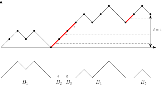
Figure 3: Splitting a partial Dyck path of level $\ell$ into $\ell+1$ non-partial Dyck paths and $\ell$ up-steps.

Let $\mathcal{B}_{j}\subseteq\mathcal{B}$ be the set of records of $\mathcal{B}$ ending with a descent annotated $(j,k)$ for some $k$ (note that $k$ may take $C_{j}$ distinct possible values by definition). Therefore, a record $R\in\mathcal{B}_{j}$ ends with a last up-step and a last descent of length $s_{j}$. The subpath $R^{\prime}$ obtained from $R$ by removing the last up-step and the last descent belongs to $\mathcal{R}_{s_{j}-1}$. Hence, the generating function of $\mathcal{B}_{j}$ is $B_{j}(y)=R_{s_{j}-1}(y)\times yC_{j}=y^{s_{j}}C_{j}B(y)^{s_{j}}$. Therefore, since a record $R\in\mathcal{B}$ is either empty (i.e. of size 0) or ends with a descent annotated $(j,k)$, we have:

$$B(y)=1+\sum_{j\in\operatorname{\mathscr{T}}}B_{j}(y)=1+\sum_{j\in\operatorname{\mathscr{T}}}C_{j}y^{s_{j}}B(y)^{s_{j}}$$ (4)

We are now ready to prove the following theorem.

Theorem 18

Algorithm Coloring_G produces at most $o\left(\left(\frac{Q(x)}{x}\right)^{t}\right)$ distinct records with $t$ "Color" lines where $Q(x)=1+\sum_{j\in\operatorname{\mathscr{T}}}C_{j}x^{s_{j}}$ and for any $x\in]0,1]$.

In practice, our aim is to minimize the value of $\frac{Q(x)}{x}$. Observe that:

Remark 19

In Theorem 18, the minimum value of $\frac{Q(x)}{x}$ is as follows:

• If $s_{j}=1$ for all $j\in\operatorname{\mathscr{T}}$, then the minimum is reached for $x=1$ and $\displaystyle\frac{Q(x)}{x}=1+\sum_{j\in\operatorname{\mathscr{T}}}C_{j}$.

• Otherwise, the minimum is reached for the unique positive root of the polynomial $\displaystyle P(x)=-1+\sum_{j\in\operatorname{\mathscr{T}}}(s_{j}-1)C_{j}x^{s_{j}}$.

Proof of Theorem 18. Let $\displaystyle\lambda=\min_{0<x\leq 1}\frac{Q(x)}{x}$. Let us prove that Algorithm Coloring_G produces at most $o(\lambda^{t})$ distinct records: it suffices to bound $r_{t}$ (the number of records of size $t$ of $\mathcal{R}$) by $o(\lambda^{t})$.

If $s_{j}=1$ for all $j\in\operatorname{\mathscr{T}}$, then $b_{t}=\left(\sum_{j\in\operatorname{\mathscr{T}}}C_{j}\right)^{t}=\left(\lambda-1\right)^{t}$ by Equation (4). It follows that $r_{t}=\sum_{0\leq\ell\leq n}{t\choose\ell}\left(\lambda-1\right)^{t-\ell}$ for sufficiently large $t$ by Equation (3). Finally, $r_{t}<(n+1)t^{n+1}\left(\lambda-1\right)^{t}$ and therefore $r_{t}=o(\lambda^{t})$.

From now on, we consider the case where $s_{j}\geq 2$ for some $j\in\operatorname{\mathscr{T}}$. As observed by Esperet and Parreau [10, Lemma 6], there is a constant $C$ (depending only on the lengths of the descents) such that $r_{t}\leq b_{t+C}$. It suffices hence to show that $b_{t}=o(\lambda^{t})$. For that purpose we make use of the smooth implicit-function schema (SIFS for short) of Meir and Moon [26] (see also Flajolet and Sedgewick’s book [15, Section VII.4.1]). Function $B(y)$ does not satisfy the SIFS and we thus introduce the function $A(y)$ defined by $A(y)=B(y^{\frac{1}{d}})-1$ where $d=\gcd\{s_{j}\ |\ j\in\operatorname{\mathscr{T}}\}$. We prove in the following that $A(y)$ satisfies the SIFS. Note that the size of Dyck paths of $\mathcal{B}$ is multiple of $d$. Therefore, we have:

$$B(y)=\sum_{t\geq 0}b_{t}y^{t}=\sum_{t\;\mbox{\scriptsize multiple of}\;d}b_{t}y^{t}.$$

Thus $B(y^{\frac{1}{d}})=1+\sum_{t\geq 1}b_{dt}y^{t}$. Hence $A(y)=\sum_{t\geq 0}a_{t}y^{t}$ with $a_{0}=0$ and $a_{t}=b_{dt}$ for $t\geq 1$. Thus $A(y)$ is analytic at 0, $a_{0}=0$, and $a_{t}\geq 0$ for all $t\geq 0$. Furthermore, note that for any sufficiently large $t$, the integer $dt$ can be written as a sum which summands belong to $\{s_{j}\ |\ j\in\operatorname{\mathscr{T}}\}$. Hence $a_{t}=b_{dt}>0$ for any sufficiently large $t>0$. It follows that $A(y)$ is aperiodic. By Equation (4), we have $A(y)=G(y,A(y))$ for the bivariate function $G$ defined by

$$G(y,z)=\sum_{j\in\operatorname{\mathscr{T}}}C_{j}y^{s_{j}/d}\left(z+1\right)^{s_{j}}.$$

Observe that

$$G(y,z)=\sum_{j\in\operatorname{\mathscr{T}}}\sum_{0\leq i\leq s_{j}}{s_{j}\choose i}C_{j}y^{s_{j}/d}z^{i},$$

and hence $G(y,z)$ is a bivariate power series satisfying the following conditions:

1. $G(y,z)$ is analytic in the domain $|y|<+\infty$ and $|z|<+\infty$.

2. Setting $G(y,z)=\sum_{m,n\geq 0}g_{m,n}y^{m}z^{n}$, the coefficients of $G$ satisfy $g_{m,n}\geq 0$, ${g_{0,0}=0}$, $g_{0,1}=0$, and $g_{\frac{s_{j}}{d},s_{j}}>0$ for the $j\in\operatorname{\mathscr{T}}$ such that $s_{j}\geq 2$.

3. There exist two positive numbers $r$ and $s$ satisfying the system of equations

   $$G(r,s)=s\leavevmode\nobreak\ \textrm{ and }\leavevmode\nobreak\ G_{z}(r,s)=1.$$

   Indeed, by setting $X=r^{1/d}(s+1)$, these two equations respectively become

   $$\sum_{j\in\operatorname{\mathscr{T}}}C_{j}X^{s_{j}}=s\leavevmode\nobreak\ \textrm{ and }\leavevmode\nobreak\ \sum_{j\in\operatorname{\mathscr{T}}}s_{j}C_{j}X^{s_{j}}=s+1.$$

   By substracting the first one to the second one, we obtain that $X$ is the unique positive root of $P(x)$ (see Remark 19) which exists. The first equation hence clearly defines $s$. In this first equation adding 1 to both sides, and then multiplying them both by $r^{1/d}$, one obtains that $r=\left(X/Q(X)\right)^{d}$.

Hence $A(y)=\sum_{t\geq 0}a_{t}y^{t}$ satisfies a smooth implicit-function schema with characteristic system $(r,s)$, see Definition 33 of A. By Theorem 34, we have that $a_{t}=O\left(t^{-\frac{3}{2}}r^{-t}\right)$. It follows that $a_{t}=o\left(r^{-t}\right)$ and $b_{t}=o\left(r^{-t/d}\right)=o\left(\left(\frac{Q(X)}{X}\right)^{t}\right)$. As $X$ is the unique positive root of $P(x)$, this concludes the proof.  $\Box$

5 Some applications of the method to graph coloring problems

In this section, we apply the framework described in Section 3 to different coloring problems. We improve several known upper bounds by at least an additive constant and sometimes also by a constant factor. More importantly, this framework allows simpler proofs with only few calculations. Indeed, directly using Theorem 12, one avoids the calculations made in Section 4.

5.1 Non-repetitive coloring

In a vertex (resp. edge) colored graph, a $2j$-repetition is a path on $2j$ vertices (resp. edges) such that the sequence of colors of the first half is the same as the sequence of colors of the second half. A coloring with no $2j$-repetition, for any $j\geq 1$, is called non-repetitive. Let $\pi(G)$ be the non-repetitive chromatic number of $G$, that is the minimum number of colors needed for any non-repetitive vertex-coloring of $G$. By extension, let $\pi_{l}(G)$ be the non-repetitive choice number of $G$. These notions were introduced by Alon et al. [1] inspired by the works on words of Thue [35]. See [19] for a survey on these parameters. Dujmović et al. [9] proved that every graph $G$ with maximum degree $\Delta$ satisfies $\pi_{l}(G)\leq\left\lceil\left(1+\frac{1}{\Delta^{\frac{1}{3}}-1}+\frac{1}{\Delta^{\frac{1}{3}}}\right)\Delta^{2}\right\rceil=\Delta^{2}+2\Delta^{\frac{5}{3}}+O(\Delta^{\frac{4}{3}})$ colors. However, their technique could provide tighter bounds from the second term on [24]. Here, we provide a simple and short proof of the following bound.

Theorem 20

Let $G$ be a graph with maximum degree $\Delta\geq 3$. We have:

$$\pi_{l}(G)\leq\left\lceil\Delta^{2}+\frac{3}{2^{\frac{2}{3}}}\Delta^{\frac{5}{3}}+\frac{2^{\frac{2}{3}}\Delta^{\frac{5}{3}}}{\Delta^{\frac{1}{3}}-2^{\frac{1}{3}}}\right\rceil=\Delta^{2}+\frac{3}{2^{\frac{2}{3}}}\Delta^{\frac{5}{3}}+O(\Delta^{\frac{4}{3}})\qquad(\mbox{Note that }\frac{3}{2^{\frac{2}{3}}}\approx 1.89)$$

Proof. To do this, let us use the framework as follows. Let $G$ be any graph with maximum degree $\Delta$, and let $n$ denote its number of vertices. In this application, the sets $\mathbb{F}(v)$ are closed upward. We directly proceed to the description of the bad events $\mathbb{B}(v)$ and the description of the required functions. Then, from the set $\mathbb{B}(v)$, we define the set $\mathbb{F}(v)$ as its upward closure.

• Let $\prec$ be any total order on the vertices of $G$. $\operatorname{\tt NextUncoloredElement}(\overline{\varphi})$ returns the first uncolored vertex according to $\prec$.

• Let $\mathbb{B}(v)$ be the set of bad events $\varphi$ anchored at $v$ such that vertex $v$ belongs to a repetition in $\varphi$. The set $\mathbb{B}(v)$ is partitioned into subsets $\mathbb{B}_{j}(v)$, for $1\leq j\leq n/2$, in such a way that in every $\varphi\in\mathbb{B}_{j}(v)$ the vertex $v$ belongs to a $2j$-repetition. Let $\operatorname{\mathscr{C}}_{j}(v)$ be the set of $2j$-vertex paths going through $v$. Each set $\mathbb{B}_{j}(v)$ is partitioned into subsets ${\mathbb{B}}_{j}^{P}(v)$ according to the path $P\in\operatorname{\mathscr{C}}_{j}(v)$ supporting the repetition. If in a bad event $\varphi\in\mathbb{B}(v)$ the vertex $v$ belongs to several repetitions, then one of the repetitions is chosen arbitrarily to set the value $j$ and the path $P$ such that $\varphi\in\mathbb{B}_{j}^{P}(v)$. Let $C_{j}=j\Delta^{2j-1}$ as this upper bounds $|\operatorname{\mathscr{C}}_{j}(v)|$. Indeed, there are $\Delta^{2j-1}$ possible paths on $2j$ vertices where $v$ has a given position, and $2j$ possible positions for $v$, but in that case every path is counted twice.

Let us prove that any partial allowed coloring $\varphi$ is a non-repetitive coloring. We proceed by induction on the number of colored vertices of $\varphi$. If there is no colored vertex, then $\varphi$ is clearly non-repetitive. Otherwise, there exists a colored vertex $v$ such that $\varphi\not\in\mathbb{F}(v)$ and uncoloring $v$ leads to a partial allowed coloring $\varphi^{\prime}$. By induction, $\varphi^{\prime}$ is non-repetitive. Thus, if $\varphi$ contains a repetition, then $v$ is necessarily involved. In such a case, we would have $\varphi\in\mathbb{F}(v)$, a contradiction.

• The function $\operatorname{\tt UncolorSetBadEvent}_{j}(v,\overline{\varphi},P)$ outputs the half of $P$ containing $v$, and thus $s_{j}=j$. By Lemma 11, this function fulfills all the requirements.

• Given $P$ and the sequence of colors of one half of $P$ (which is colored in $\varphi^{\prime}$), it is easy to recover the sequence of colors of the other half of $P$, and so $\operatorname{\tt RecoverBadEvent}_{j}(v,X,P,\varphi^{\prime})$ is well-defined.

Consider now

$$Q(x)=1+\sum_{1\leq j\leq n/2}C_{j}x^{s_{j}} = 1+\sum_{1\leq j\leq n/2}j\Delta^{2j-1}x^{j}$$

$$< 1+\frac{\Delta x}{(\Delta^{2}x-1)^{2}}\mbox{\hskip 28.45274pt if }\ \ x<\frac{1}{\Delta^{2}}$$

By setting $X=\frac{1}{\Delta^{2}}-\left(\frac{2}{\Delta^{7}}\right)^{\frac{1}{3}}$ ($X>0$ as $\Delta\geq 3$), one obtains that

$$\frac{Q(X)}{X} < \Delta^{2}+\frac{3}{2^{\frac{2}{3}}}\Delta^{\frac{5}{3}}+\frac{2^{\frac{2}{3}}\Delta^{\frac{5}{3}}}{\Delta^{\frac{1}{3}}-2^{\frac{1}{3}}}$$

By Theorem 12, $G$ admits an allowed coloring (hence a non-repetitive coloring) with $\left\lceil Q(X)/X\right\rceil$ colors. This concludes the proof of the theorem. $\Box$

An edge-coloring is called non-repetitive if, for every path with an even number of edges, the sequence of colors of the first half differs from the sequence of colors of the second half. The minimim number of colors needed to have such a coloring on the edges of $G$ is called the Thue index of $G$, and is denoted by $\pi^{\prime}(G)$. By extension, let $\pi^{\prime}_{l}(G)$ be the Thue choice index of $G$. Alon et al. [1] proved that every graph $G$ with maximum degree $\Delta$ satisfies $\pi^{\prime}(G)\leq c\Delta^{2}$ with $c=2e^{16}+1$. We can prove:

Theorem 21

Let $G$ be a graph with maximum degree $\Delta\geq 3$. Then

$$\pi^{\prime}_{l}(G)\leq\Delta^{2}+2^{\frac{4}{3}}\Delta^{\frac{5}{3}}+O(\Delta^{\frac{4}{3}}).$$

The only difference with the vertex case is that $C_{j}=2j\Delta^{2j-1}$.

5.2 Facial Thue vertex-coloring

We consider in this subsection a slight variation of non-repetitive coloring which applies to plane graphs (i.e. embedded planar graphs). Here the restriction on repetitions only applies on facial paths. More formally, consider a plane graph $G$. A facial path of $G$ is a path on consecutive vertices on the boundary walk of some face of $G$. A vertex-coloring of $G$ is said to be facially non-repetitive if none of the facial paths is a repetition. The notion can be extended to list coloring. Let $\pi_{f}(G)$ (resp. $\pi_{fl}(G)$) denote the facial Thue chromatic number (resp. facial Thue choice number) that is the minimum integer $k$ such that $G$ is facially non-repetitively $k$-colorable (resp. $k$-choosable). Barát and Czap [6] proved that for any plane graph $G$, $\pi_{f}(G)\leq 24$. Whether the facial Thue choice number of plane graphs could be bounded from above by a constant is still an open question. Recently Przybyło et al. [32] proved that, if $G$ is a plane graph of maximum degree $\Delta$, then $\pi_{fl}(G)\leq 5\Delta$, and asymptotically, $\pi_{fl}(G)\leq(2+o(1))\Delta$. We improve these upper bounds as follows:

Theorem 22

Let $G$ be a plane graph with maximum degree $\Delta\geq 2$. Then,

$$\pi_{fl}(G)\leq\left\lceil\Delta+4\sqrt{\Delta}+3\right\rceil$$

Proof. Let $G$ be a plane graph with maximum degree $\Delta$. In this application, the sets $\mathbb{F}(v)$ are closed upward. We directly proceed to the description of the bad events $\mathbb{B}(v)$ and the description of the required functions. Then, from the set $\mathbb{B}(v)$, we define the set $\mathbb{F}(v)$ as its upward closure.

• As previously, let $\prec$ be any total order on the vertices of $G$. $\operatorname{\tt NextUncoloredElement}(\overline{\varphi})$ returns the first uncolored vertex according to $\prec$.

• For $1\leq j\leq\left\lfloor n/2\right\rfloor=p$, let $\mathbb{B}_{j}(v)$ be the set of bad events $\varphi$ such that vertex $v$ belongs to a repetition on a facial $2j$-vertex path $P$. Let $\operatorname{\mathscr{C}}_{j}(v)$ be the set of facial $2j$-vertex paths going through $v$. Each set $\mathbb{B}_{j}(v)$ is partitioned into sets $\mathbb{B}^{P}_{j}(v)$, for every $P\in\operatorname{\mathscr{C}}_{j}(v)$, according to the path $P$ supporting the repetition. The number of obtained classes is such that we set $C_{1}=\Delta$ and $C_{j}=2j\Delta$ for $j\geq 2$. Indeed, there are at most $\Delta$ possible faces for containing $P$, and $2j$ positions for $v$ in $P$.

Let us prove that any partial allowed coloring $\varphi$ is a facial non-repetitive coloring. Proceed by induction on the number of colored vertices of $\varphi$. Either $\varphi$ has no colored vertex and it is facially non-repetitive, or there exists a colored vertex $v$ such that $\varphi\not\in\mathbb{F}(v)$ and uncoloring $v$ leads to a partial allowed coloring $\varphi^{\prime}$, that is hence facial non-repetitive. Thus, if $\varphi$ contains a facial repetition, then $v$ is necessarily involved. In such a case, we would have $\varphi\in\mathbb{F}(v)$, a contradiction.

• The function $\operatorname{\tt UncolorSetBadEvent}_{j}(v,\overline{\varphi},P)$ outputs the half of the path $P$ containing $v$, and thus $s_{j}=j$. By Lemma 11, this function fulfills all the requirements.

• Given $P$ and the sequence of colors of the colored half of $P$, it is easy to recover the sequence of colors of the uncolored half of $P$, and so $\operatorname{\tt RecoverBadEvent}_{j}(v,X,P,\varphi^{\prime})$ is well-defined.

Consider now

$$Q(x)=1+\sum_{1\leq j\leq n/2}C_{j}x^{s_{j}} = 1+\Delta x+\sum_{2\leq j\leq p}2j\Delta x^{j}$$

$$< 1+\Delta x+2\Delta x^{2}\frac{2-x}{(x-1)^{2}}\quad\mbox{\hskip 28.45274pt for }x<1$$

By setting $X=\frac{1}{2\sqrt{\Delta}}$, and as $\Delta\geq 2$ one obtains that

$$\frac{Q(X)}{X} < \Delta+4\sqrt{\Delta}+3$$

By Theorem 12, $G$ admits an allowed coloring (hence a facial non-repetitive coloring) with $\left\lceil Q(X)/X\right\rceil$ colors. This concludes the proof of the theorem. $\Box$

Piotr Micek recently announced that this theorem can be improved asymptotically as for any plane graph $G$, $\pi_{fl}(G)\leq O(\log\Delta)$ [24].

5.3 Facial Thue edge-coloring

Consider the facial Thue choice index $\pi^{\prime}_{fl}(G)$ of a plane graph $G$, that is the minimum integer $k$ such that $G$ is facially non-repetitively edge $k$-choosable. Schreyer and Škrabul’áková [33] proved that plane graphs have bounded facial Thue choice index, more precisely $\pi^{\prime}_{fl}(G)\leq 291$. Recently Przybyło [31] improved that bound to 12. To obtain that upper bound with our framework, it is sufficient to consider as bad events the partial colorings having a facial $2j$-repetition (for any $j\geq 1$) with costs $C_{j}=4j$ since an edge belongs to at most $4j$ facial $2j$-edge paths.

Let us explain a way to improve that upper bound. The idea is that at each step the algorithm chooses the edge $e$ to be colored in such a way that $e$ is facially adjacent to an uncolored edge $e^{\prime}$. Therefore, if at some step the algorithm colors such an edge $e$, then this edge belongs to at most $1+2j$ facial $2j$-edge paths going through colored edges (one path in the face incident to $e$ and $e^{\prime}$ and $2j$ paths on the other face incident to $e$). However, such an edge $e$ does not always exist. For example if the algorithm has colored all the graph $G$ but one edge, then this edge may belong to $4j$ colored facial $2j$-edge paths. We manage to use this trick to obtain the improved bound of 10.

We will need the following definition. Given a plane graph $G$, its medial graph $M(G)$ is defined as follows:

• its vertex set is the set of edges of $G$;

• there is an edge $uv$ between the vertices $u$ and $v$ of $M(G)$ if and only if the corresponding edges in $G$ are facially adjacent (i.e. adjacent and both incident to the same face).

Theorem 23

For any plane graph $G$, any edge $e^{*}$ of $G$, and any assignment of lists of size $9$, there exists a partial facial Thue edge-coloring of $G$ where all the edges except $e^{*}$ are colored.

Proof. Let $G$ be a plane graph with maximum degree $\Delta$, and let $e^{*}$ be any edge of $G$. In this application, we want to ensure that at each iteration of the main loop the current edge to color is facially adjacent to (at least) one uncolored edge. This leads us to sets $\mathbb{F}(e)$ that are not closed upward. Hence they need to be described with care. For a given edge $e$, the set $\mathbb{F}(e)$ contains the partial colorings with a facial repetition involving $e$, and the partial colorings where the set of uncolored edges (i.e. vertices of $M(G)$), including $e^{*}$, induces a disconnected graph in $M(G)$. Hence the set of allowed colorings is the set of partial colorings with no facial repetition, and where uncolored edges, including $e^{*}$, induce a connected graph in $M(G)$.

We conveniently define $\operatorname{\tt NextUncoloredElement}$ in order to avoid bad events dealing with the case where uncolored edges induce a disconnected graph in $M(G)$.

• For any set $X\subseteq E(G)$ such that $e^{*}\in X$, and such that $M(G)[X]$ is connected, the edge $e=\operatorname{\tt NextUncoloredElement}(E(G)\setminus X)$ must be such that $M(G)[X-e]$ is connected. Hence, $e$ may be chosen among leaves of a spanning tree of $M(G)[X]$ rooted at $e^{*}$.

Hence with that definition of $\operatorname{\tt NextUncoloredElement}$ we have that for a given edge $e$, the set of bad events $\mathbb{B}(e)$ contains the partial colorings with a facial repetition involving $e$, where $e$ is facially adjacent to an uncolored edge $e^{\prime}$ (its parent in the spanning tree described above, which might be $e^{*}$), and where the set of uncolored edges induces a connected graph in $M(G)$. Let us introduce the bad event types and classes:

• For $1\leq j\leq p=\left\lfloor n/2\right\rfloor$, let $\mathbb{B}_{j}(e)$ be the set of bad events anchored at $e$ such that $e$ has an uncolored facially adjacent edge $e^{\prime}$, and $e$ belongs to a repetition on a (colored) facial $2j$-edge path $P$.

  The partition into classes is not obvious. Let $e_{1},e_{2},e_{3}$ and $e_{4}$ be the (at most four) edges of $G$ facially adjacent to $e$, and let $e^{\prime}\in\{e_{1},e_{2},e_{3},e_{4}\}$ be the uncolored one with smallest index. Let us now partition $\mathbb{B}_{j}(e)$ into sets $\mathbb{B}_{j}^{e^{\prime},P}(e)$ according to the uncolored edge $e^{\prime}$ and the path $P$ supporting the repetition. We have seen earlier that given an edge $e^{\prime}$ there are at most $1+2j$ possible paths $P$. As there are up to four possibilities for $e^{\prime}$ this partition has $4+8j$ parts, but the cases where $e^{\prime}$ has distinct values are independent. Let us hence merge these parts as follow. Let $\mathbb{B}_{j}^{k}(e)$, for $1\leq k\leq 1+2j$, be the union of $\mathbb{B}_{j}^{e_{1},P_{1}}(e)$, $\mathbb{B}_{j}^{e_{2},P_{2}}(e)$, $\mathbb{B}_{j}^{e_{3},P_{3}}(e)$ and $\mathbb{B}_{j}^{e_{4},P_{4}}(e)$, for some choice of paths $P_{1}$, $P_{2}$, $P_{3}$ and $P_{4}$. The obtained partition has $C_{j}=1+2j$ classes.

• Given the set of colored edges $\overline{\varphi}$ of some bad event $\varphi\in\mathbb{B}_{j}(e)$, one can determine the facially adjacent uncolored edge $e^{\prime}$. Hence given (also) the class $k$ such that $\varphi\in\mathbb{B}_{j}^{k}(e)$, one can determine the path $P$ supporting the repetition. The function $\operatorname{\tt UncolorSetBadEvent}_{j}(e,\overline{\varphi},k)$ outputs the half of the path $P$ containing $e$, and thus $s_{j}=j$. Note that as the edges of $P$ are incident to the same face, and as $e$ and $e^{\prime}$ are facially adjacent, uncoloring this set of edges leads to a partial coloring that has no repetition and such that the uncolored edges induce a connected graph in $M(G)$, hence an allowed coloring (as required).

• Using again the fact that $P$ can be retrived from $\overline{\varphi}$ ($=X$ here) and $k$, one can easily design a function $\operatorname{\tt RecoverBadEvent}_{j}(v,X,k,\varphi_{i+1})$.

Consider now

$$Q(x)=1+\sum_{1\leq j\leq n/2}C_{j}x^{s_{j}} = 1+\sum_{1\leq j\leq n/2}(1+2j)x^{j}$$

$$< \frac{1}{1-x}+\frac{2x}{(1-x)^{2}}\mbox{\hskip 28.45274pt if }\ \ x<1$$

By setting $X=\frac{\sqrt{17}-3}{4}$, one obtains that $Q(X)/X<9$. Hence by Theorem 12, $G$ admits a partial allowed 9-coloring (hence a partial facial Thue edge-coloring) where $e^{*}$ is the onlyuncolored edge. This concludes the proof of the theorem. $\Box$

Given Theorem 23, it seems likely that $\pi^{\prime}_{fl}(G)\leq 9$ for any plane graph $G$. Actually one can show that it is the case if $G$ has an edge $e^{*}$ incident to two faces of small sizes. Unfortunately we do not achieve this bound here, but we prove:

Corollary 24

For any plane graph $G$, $\pi^{\prime}_{fl}(G)\leq 10$.

Proof. For a given $G$, pick an arbitrary edge $e^{*}\in E(G)$ and an arbitrary color $c\in L(e^{*})$. For all the other edges of $G$, remove color $c$ from their list. Now all these lists have size at least 9. By Theorem 23, it is possible to color all the edge of $G$ except $e^{*}$, avoiding facial repetitions. Then coloring $e^{*}$ with $c$ cannot create any repetition, as $c$ does not appear elsewhere in $G$. $\Box$

Remark 25

Note that in the proof of Theorem 23 we only use the fact that edges are adjacent to at most two faces, and thus it extends to any graph embedded on any surface. Hence, Theorem 23 and Corollary 24, both extend to arbitrary surface.

5.4 Generalised acyclic coloring

Let $r\geq 3$ be an integer. An $r$-acyclic vertex-coloring is a proper vertex-coloring such that every cycle $C$ uses at least $\min(|C|,r)$ colors. This generalisation of the notion of acyclic coloring (the $r=3$ case) was introduced by Gerke et al. in the context of edge-coloring [16] and then by Greenhill and Pikhurko in the context of vertex-coloring [17]. Let $A_{r}(G)$ be the minimum number of colors in any $r$-acyclic vertex-coloring of $G$. By extension, let $A_{r}^{l}(G)$ be the $r$-acyclic choice number of $G$. Greenhill and Pikhurko [17] proved in particular that, for $r\geq 4$ and $\Delta\geq 3$, every graph $G$ with maximum degree $\Delta$ satisfies $A_{r}(G)\leq c\Delta^{\lfloor r/2\rfloor}$ where $c=2^{(r+2)/3}r(r+2)$. We reduce this constant factor as follows.

Theorem 26

Let $G$ be a graph with maximum degree $\Delta\geq 3$. For any $r\geq 4$, we have that $A_{r}^{l}(G)\leq\Delta^{\left\lfloor r/2\right\rfloor}+O\left(\Delta^{(r+1)/3}\right)$.

In the following, all the defined events are strongly inspired by those defined by Greenhill and Pikhurko [17]. Let $G$ be any graph with maximum degree $\Delta$, and let $n$ denote its number of vertices. Let $\prec$ be any total order on the vertices of $G$. $\operatorname{\tt NextUncoloredElement}(\overline{\varphi})$ returns the first uncolored vertex according to $\prec$. In this application, the sets $\mathbb{F}(v)$ are closed upward. We hence use Lemma 11, to ensure that each function $\operatorname{\tt UncolorSetBadEvent}$ fulfills all the requirements. We proceed now to the description of the bad events (the sets $\mathbb{F}(v)$ being deduced from $\mathbb{B}(v)$), and the description of the required functions. We distinguish two cases according to $r$’s parity.

5.4.1 Case $r$ even

Set $r=2\ell$ with $\ell\geq 2$. We consider the following sets of bad events anchored at vertex $v$:

• Let $\mathbb{B}_{1}(v)$ be the set of bad events $\varphi$ where “there exists a vertex $u$ at distance at most $\ell$ (from $v$) having the same color as $v$”. Let $\operatorname{\mathscr{C}}_{1}(v)$ be the set of vertices $u$ at distance at most $\ell$ from $v$. As $|\operatorname{\mathscr{C}}_{1}(v)|\leq\sum_{i=1}^{\ell}\Delta(\Delta-1)^{i-1}=\frac{\Delta((\Delta-1)^{\ell}-1)}{\Delta-2}\leq\Delta^{\ell}$ we set $C_{1}=\Delta^{\ell}$. Each set $\mathbb{B}_{1}(v)$ is partitioned into classes $\mathbb{B}_{1}^{u}(v)$, for every vertex $u\in\operatorname{\mathscr{C}}_{1}(v)$, according to the vertex $u$ that is colored like $v$. $\operatorname{\tt UncolorSetBadEvent}_{1}(v,\overline{\varphi},u)$ outputs the vertex $v$, and thus $s_{1}=1$. In addition, $\operatorname{\tt RecoverBadEvent}_{1}(v,X,u,\varphi^{\prime})$ outputs the partial coloring $\varphi$ obtained from $\varphi^{\prime}$ by coloring $v$ with color $\varphi^{\prime}(u)$.

Here it is clear that an allowed coloring is a distance $\ell$ proper coloring. Furthermore, as $r=2\ell$, cycles $C$ of length at most $r+1$ will receive $|C|$ distinct colors.

• Let $\mathbb{B}_{2}(v)$ be the set of bad events $\varphi$ where “$v$ belongs to a path $P$ on $r+2$ vertices such that $v$ and two other colored vertices, say $a$, $b$, have colors that already appear on $P\setminus\{v,a,b\}$”. Let us define a partition of $\mathbb{B}_{2}(v)$. Consider the set $\operatorname{\mathscr{C}}_{2}(v)$ formed by all tuples $(P,a,b,v^{\prime},a^{\prime},b^{\prime})$ such that $P$ is a path on $r+2$ vertices containing vertices $v,a,b,v^{\prime},a^{\prime},b^{\prime}$ where $|\{v,a,b\}|=3$, $1\leq|\{v^{\prime},a^{\prime},b^{\prime}\}|\leq 3$ and $\{v,a,b\}\cap\{v^{\prime},a^{\prime},b^{\prime}\}=\emptyset$. Let $\mathbb{B}_{2}^{(P,a,b,v^{\prime},a^{\prime},b^{\prime})}(v)\subset\mathbb{B}_{2}(v)$ be the class of bad events $\varphi$ where “both $v$ and $v^{\prime}$ have the same color, both $a$ and $a^{\prime}$ have the same color, and both $b$ and $b^{\prime}$ have the same color”. Let us count the number of such classes. First observe that $v$ belongs to at most $\frac{r+2}{2}\Delta(\Delta-1)^{r}$ paths on $r+2$ vertices. Now observe that there are at most $r+2$ possible choices for each vertex $a,b,v^{\prime},a^{\prime},b^{\prime}$. Hence let us set $C_{2}=\frac{1}{2}(r+2)^{6}\Delta^{r+1}$. $\operatorname{\tt UncolorSetBadEvent}_{2}(v,\overline{\varphi},(P,a,b,v^{\prime},a^{\prime},b^{\prime}))$ outputs the set $\{v,a,b\}$, and thus $s_{2}=3$. In addition, $\operatorname{\tt RecoverBadEvent}_{2}(v,X,(P,a,b,v^{\prime},a^{\prime},b^{\prime}),\varphi^{\prime})$ outputs the partial coloring $\varphi$ obtained from $\varphi^{\prime}$ by coloring vertices $v$, $a$ and $b$ respectively with colors $\varphi^{\prime}(v^{\prime})$, $\varphi^{\prime}(a^{\prime})$ and $\varphi^{\prime}(b^{\prime})$.

These bad events imply that in an allowed coloring, cycles of length at least $r+2$ contain at least $r$ colors. Hence an allowed coloring is also a generalised $r$-acyclic coloring. Consider now

$$Q(x)=1+\sum_{1\leq j\leq n/2}C_{j}x^{s_{j}} = 1+C_{1}x+C_{2}x^{3}$$

By setting $X=\left(\frac{1}{2C_{2}}\right)^{\frac{1}{3}}$ one obtains that

$$\frac{Q(X)}{X} = C_{1}+\frac{3}{2^{\frac{2}{3}}}C_{2}^{\frac{1}{3}}$$

$$= \Delta^{\ell}+\frac{3}{2}(r+2)^{2}\Delta^{(r+1)/3}$$

By Theorem 12, $G$ admits an allowed coloring (hence a generalised $r$-acyclic coloring) with $\left\lceil Q(X)/X\right\rceil$ colors. This concludes the proof of the theorem for $r$ even.

5.4.2 Case $r$ odd

The odd case is similar to the even case. Let $r=2\ell+1$ with $\ell\geq 2$. Let us use again the two types of bad events defined above. Now, type 1 bad events are sufficient to deal with cycles of length at most $r$. Type $2$ bad events are still sufficient to deal with cycles of length at least $r+2$. It remains to deal with cycles of length $r+1$. Type 1 bad events forbid some kinds of length $r+1$ cycles. As $r+1=2\ell+2$, the cycles of length $r+1$ that are not forbidden by type 1 bad events are those where each color appears only once, or where colors appearing several times, do it on antipodal vertices. We thus add two other bad event types to deal with this kind of cycles of length $r+1$.

A pair of vertices $\{u,u^{\prime}\}$ is said to be special if $u$ and $u^{\prime}$ are at distance exactly $\ell+1$ and if there exist at least $\Delta^{\frac{\ell+1}{3}}$ paths of length $\ell+1$ linking $u$ and $u^{\prime}$. Consider the two following new sets of bad events:

• Let $\mathbb{B}_{3}(v)$ be the set of bad events $\varphi$ where “there exists a special pair $\{v,u\}$ such that $v$ and $u$ have the same color”. Let $\operatorname{\mathscr{C}}_{3}(v)$ be the set of vertices $u$ such that $\{v,u\}$ is a special pair. Each set $\mathbb{B}_{3}(v)$ is partitioned into classes $\mathbb{B}_{3}^{u}(v)$ according to the vertex $u$ colored like $v$. As there are at most $\Delta^{\ell+1}$ paths of length $\ell+1$ starting from $v$, there exist at most $\Delta^{\frac{2}{3}(\ell+1)}=\Delta^{(r+1)/3}=C_{3}$ such classes. Functions $\operatorname{\tt UncolorSetBadEvent}_{3}$ and $\operatorname{\tt RecoverBadEvent}_{3}$ are defined similarly to the first type of bad events, with $s_{3}=1$.

• Let $\mathbb{B}_{4}(v)$ be the set of bad events $\varphi$ where “$v$ belongs to a cycle $C$ of length $r+1=2\ell+2$ such that $v$ and its antipodal vertex $v^{\prime}$ (on $C$) have the same color, are at distance $\ell+1$ from each other but do not form a special pair, and such that $C$ contains another pair of antipodal vertices $\{u,u^{\prime}\}$ having the same color”. Let $\operatorname{\mathscr{C}}_{4}(v)$ be the set of couples $(C,u)$ such that $C$ is a $(r+1)$-cycle containing $v$ and $u$ as non-antipodal vertices. Each set $\mathbb{B}_{4}(v)$ is partitioned into classes ${\mathbb{B}}_{4}^{(C,u)}(v)$, for every $(C,u)\in\operatorname{\mathscr{C}}_{4}(v)$. There exist at most $\ell\Delta^{\frac{4}{3}(\ell+1)}=\ell\Delta^{\frac{2}{3}(r+1)}=C_{4}$ such classes. Indeed, there are $\Delta^{\ell+1}$ choices for vertex $v^{\prime}$ and the path from $v$ to $v^{\prime}$; as $v$ and $v^{\prime}$ do not form a special pair, there are $\Delta^{\frac{1}{3}(\ell+1)}$ choices for the path from $v^{\prime}$ back to $v$; and finally there are $\ell$ possibilities for the pair $\{u,u^{\prime}\}$ of antipodal vertices. The function $\operatorname{\tt UncolorSetBadEvent}_{4}(v,\overline{\varphi},(C,u))$ outputs $\{v,u\}$, so $s_{4}=2$, and $\operatorname{\tt RecoverBadEvent}_{4}$ clearly exists.

One can check that these two new types of bad events handle the remaining cycles of length $r+1$ colored with less than $r$ colors. This ensures us that allowed colorings are generalised $r$-acyclic colorings. Consider now

$$Q(x)=1+\sum_{1\leq j\leq n/2}C_{j}x^{s_{j}} = 1+C_{1}x+C_{2}x^{3}+C_{3}x+C_{4}x^{2}$$

By setting $X=\frac{1}{\Delta^{(r+1)/3}}$ one obtains that

$$\frac{Q(X)}{X} = \Delta^{\ell}+\Delta^{(r+1)/3}+\Delta^{(r+1)/3}\left(1+\ell+\frac{1}{2}(r+2)^{6}\right)$$

$$= \Delta^{\ell}+\Delta^{(r+1)/3}\left(2+\ell+\frac{1}{2}(r+2)^{6}\right)$$

By Theorem 12, $G$ admits an allowed coloring (hence a generalised $r$-acyclic coloring) with $\left\lceil Q(X)/X\right\rceil$ colors. This concludes the proof of the theorem for $r$ odd.

5.5 Colorings with restrictions on pairs of color classes

For many graph colorings, the color classes are asked to induce independent sets while another property is asked to each pair of color classes. Aravind and Subramanian [4] introduced a general definition that captures many known colorings. In their definition, restrictions may apply to any $\ell$ color classes, for any $\ell\geq 2$. Let us restrict ourselves to the case $\ell=2$.

Given a family $\mathcal{F}$ of connected bipartite graphs, a $(2,\mathcal{F})$-subgraph coloring of $G$ is a proper coloring of $V(G)$ such that the subgraph of $G$ induced by any two color classes does not contain any isomorphic copy of $H$ as a subgraph, for each $H\in\mathcal{F}$. Denote by $\chi_{2,\mathcal{F}}(G)$ the minimum number of colors used by any $(2,\mathcal{F})$-subgraph coloring of $G$. Denote by $\chi_{2,\mathcal{F}}(\Delta)$ the maximum value of $\chi_{2,\mathcal{F}}(G)$ for any graph $G$ having maximum degree at most $\Delta$. For example, when $\mathcal{F}$ is the family of even cycles, $(2,\mathcal{F})$-subgraph coloring is the usual acyclic vertex-coloring.

Using random graphs, Aravind and Subramanian [4] showed the following lower bound on $\chi_{2,\mathcal{F}}(\Delta)$.

Theorem 27 (Aravind and Subramanian [4])

Given a connected bipartite graph $H$ with $m$ edges ($m\geq 2$), we have

$$\chi_{2,\{H\}}(\Delta)=\Omega\left(\frac{\Delta^{\frac{m}{m-1}}}{(\log\Delta)^{1/(m-1)}}\right)$$

Hence, the same bound applies to $\chi_{2,\mathcal{F}}(\Delta)$ for any family $\mathcal{F}$ containing a graph $H$ with $m$ edges.

The same authors later showed that this lower bound is almost tight. Let $m\geq 2$ be an integer and let $\mathcal{F}$ be a family of connected bipartite graphs such that all the graphs have at least $m$ edges.

Theorem 28 (Aravind and Subramanian [5])

For some constant $C$ depending only on $\mathcal{F}$, we have

$$\chi_{2,\mathcal{F}}(\Delta)\leq C\Delta^{\frac{m}{m-1}}$$

Partition the graphs in $\mathcal{F}$ according to their number of vertices. Let $\mathcal{F}_{v}^{\leq m}$ (resp. $\mathcal{F}_{v}^{>m}$) denote the subset of $\mathcal{F}$ with graphs on at most $m$ vertices (resp. more that $m$ vertices). Let also $k_{v}^{\leq m}=|\mathcal{F}_{v}^{\leq m}|$. We consider another parition of $\mathcal{F}$ according to the number of edges in each graph. Let $\mathcal{F}_{e}^{m}$ (resp. $\mathcal{F}_{e}^{>m}$) denote the subset of $\mathcal{F}$ with graphs on exactly $m$ edges (resp. more that $m$ edges); and let $k_{e}^{m}=|\mathcal{F}_{e}^{m}|$.

The constant $C$ mentionned in Theorem 27 is either $64(m+1)^{3}k_{v}^{\leq m}$ or $128(m+1)^{3}$ according to whether $k_{v}^{\leq m}>0$ or not. Following the approach of Aravind and Subramanian, we improve $C$ as follows.

Theorem 29

We have

$$\chi_{2,\mathcal{F}}(\Delta) < (k_{v}^{\leq m}+71)(m+1)\Delta^{\frac{m}{m-1}}$$ (5)

$$\chi_{2,\mathcal{F}}(\Delta) < \left(k_{e}^{m}+1+o(1)\right)(m+1)\Delta^{\frac{m}{m-1}}$$ (6)

Proof. Let us use the framework described in Section 3 as follows. Let $\mathcal{F}=\left\{H_{1},H_{2},\ldots\right\}$. Let us also denote by $n_{i}$ and $m_{i}$ the number of vertices and edges in the forbidden graph $H_{i}$ for each $i$ (recall $m_{i}\geq m$). For convenience, we introduce the value $\gamma=\frac{m}{m-1}$. Let $G$ be any graph with maximum degree $\Delta$, and let $n$ denote its number of vertices. As in this application, the sets $\mathbb{F}(v)$ are closed upward we directly proceed to the description of the bad events (as $\mathbb{F}(v)$ is deduced from $\mathbb{B}(v)$), and the description of the required functions.

• Let $\prec$ be any total order on the vertices of $G$. $\operatorname{\tt NextUncoloredElement}(\overline{\varphi})$ returns the first uncolored vertex according to $\prec$.

• Let $\mathbb{B}_{E}(v)$ be the set of bad events $\varphi$ anchored at $v$ such that vertex $v$ belongs to a monochromatic edge $uv$ (in $\varphi$). Let $\operatorname{\mathscr{C}}_{E}(v)=N(v)$. Let us partition $\mathbb{B}_{E}(v)$ into classes $\mathbb{B}_{E}^{u}(v)$ according to which edge $uv$ is monochromatic in $\varphi$, for $u\in\operatorname{\mathscr{C}}_{E}(v)$. Clearly $|\operatorname{\mathscr{C}}_{E}(v)|\leq\Delta$, thus let $C_{E}=\Delta$.

From here it is clear that an allowed coloring is proper.

• The function $\operatorname{\tt UncolorSetBadEvent}_{E}(v,\overline{\varphi},u)$ outputs the singleton $\{v\}$ and thus $s_{E}=1$. By Lemma 11, this function fulfills all the requirements.

• $\operatorname{\tt RecoverBadEvent}_{E}(v,X,u,\varphi^{\prime})$ outputs the partial coloring $\varphi\in\mathbb{B}_{E}^{u}(v)$ obtained from $\varphi^{\prime}$ by coloring $v$ with color $\varphi^{\prime}(u)$.

Following the approach of Aravind and Subramanian [5], we extend the notion of special pairs introduced by Alon et al. [2] to bigger sets. For any $j\geq 2$, a $j$-set $S$ of $G$ (i.e. a set of size $j$) is special if the set $X=\bigcap_{v\in S}N(v)$ has size greater than $\Delta^{j-\gamma(j-1)}$. Let us define the corresponding bad events.

• For $2\leq j<n$, let $\mathbb{B}_{{j\cdot{\rm Set}}}(v)$ be the set of bad events $\varphi$ anchored at $v$ such that vertex $v$ belongs to a monochromatic special $j$-set $S$. Let $\operatorname{\mathscr{C}}_{j\cdot{\rm Set}}(v)$ be the set of special $j$-sets containing $v$. Let us partition $\mathbb{B}_{j\cdot{\rm Set}}(v)$ into classes $\mathbb{B}_{j\cdot{\rm Set}}^{S}(v)$ according to which special $j$-set $S\in\operatorname{\mathscr{C}}_{j\cdot{\rm Set}}(v)$ is monochromatic. By Claim 30, the number of classes is at most $\frac{1}{(j-1)!}\Delta^{\gamma(j-1)}=C_{j\cdot{\rm Set}}$.

  Claim 30

  Any vertex $v$ of $G$ belongs to less than $\frac{1}{(j-1)!}\Delta^{\gamma(j-1)}$ special $j$-sets, for any $j\geq 2$.

  Proof. Observe that $v$ belongs to $\Delta{\Delta-1\choose j-1}$ stars (on $j+1$ vertices) centered in $N(v)$ having $j-1$ leaves in $N^{2}(v)$ (first choose a center and then $j-1$ of its neighbors). Now the $j$ leaves of such a star are contained in at most one special $j$-set of $v$. On the other hand, a special $j$-set containing $v$ covers more than $\Delta^{j-\gamma(j-1)}$ of these stars. Hence $v$ belongs to less than $\Delta{\Delta-1\choose j-1}\times\Delta^{\gamma(j-1)-j}<\frac{1}{(j-1)!}\Delta^{\gamma(j-1)}$ special $j$-sets. $\Box$

From here it is clear that in an allowed coloring there will be no monochromatic special $j$-set.

• For $2\leq j<n$, let the function $\operatorname{\tt UncolorSetBadEvent}_{j\cdot{\rm Set}}(v,\overline{\varphi},S)$ outputs a $(j-1)$-subset of $S$ containing $v$ ; thus $s_{j\cdot{\rm Set}}=j-1$. Again by Lemma 11, this function fulfills all the requirements.

• If $\operatorname{\tt RecoverBadEvent}_{j}(v,X,S,\varphi^{\prime})$ is called, then there is only one vertex of $S$ colored in $\varphi^{\prime}$, say $w$. Hence $\operatorname{\tt RecoverBadEvent}_{j}(v,X,S,\varphi^{\prime})$ outputs the partial coloring obtained from $\varphi^{\prime}$ by coloring all the vertices of $S$ with $\varphi^{\prime}(w)$.

As proposed in [5], one bad event type can deal with all the graphs in $\mathcal{F}_{v}^{>m}\subseteq\mathcal{F}$ the set of forbidden graphs having more than $m$ vertices.

• Let $\mathbb{B}_{\mathcal{F}_{v}^{>m}}(v)$ be the set of bad events $\varphi$ anchored at $v$ such that vertex $v$ belongs to a connected properly bicolored subgraph $I$ on $m+1$ vertices. Note that such subgraph $I$ of $G$ is not necessarily isomorphic to a graph of $\mathcal{F}_{v}^{>m}$. However this type of bad events deal with all the graphs of $\mathcal{F}$ with at least $m+1$ vertices. Let $\operatorname{\mathscr{C}}_{\mathcal{F}_{v}^{>m}}(v)$ be the set of all connected bipartite graphs $I$ on $m+1$ vertices that contain vertex $v$. We partition $\mathbb{B}_{\mathcal{F}_{v}^{>m}}(v)$ into classes $\mathbb{B}_{\mathcal{F}_{v}^{>m}}^{I}(v)$ according to the bicolored subgraph $I$. By the proof of Lemma 2.4 in [4] we have that the number of classes, $|\operatorname{\mathscr{C}}_{\mathcal{F}_{v}^{>m}}(v)|\leq(m+1)4^{m+1}\Delta^{m}=C_{\mathcal{F}_{v}^{>m}}$.

From here it is clear that in an allowed coloring there will be no properly bicolored copy of any $H_{i}\in\mathcal{F}$ with more than $m$ vertices.

• The function $\operatorname{\tt UncolorSetBadEvent}_{\mathcal{F}_{v}^{>m}}(v,\overline{\varphi},I)$ outputs a $(m-1)$-subset of $V(I)$ containing $v$ (recall $I$ is a properly bicolored subgraph on $m+1$ vertices), such that the two remaining vertices $v_{1}$ and $v_{2}$ are adjacent (and thus have distinct colors). Note that $s_{\mathcal{F}_{v}^{>m}}=m-1$. Again by Lemma 11, this function fulfills all the requirements.

• If $\operatorname{\tt RecoverBadEvent}_{\mathcal{F}_{v}^{>m}}(v,X,I,\varphi^{\prime})$ is called, then there are only two adjacent vertices of $I$, $v_{1}$ and $v_{2}$, colored in $\varphi^{\prime}$. Hence $\operatorname{\tt RecoverBadEvent}_{\mathcal{F}_{v}^{>m}}(v,X,I,\varphi^{\prime})$ outputs the partial coloring obtained from $\varphi^{\prime}$ by properly extending the 2-coloring of $v_{1}$ and $v_{2}$ to the whole $I$.

We define a new bad event type for each graph $H_{i}\in\mathcal{F}_{v}^{\leq m}$, that is each graph of $\mathcal{F}$ with at most $m$ vertices. Let $V_{1}$ and $V_{2}$ be the two independent sets partitioning $V(H_{i})$.

• Let $\mathbb{B}_{Hi}(v)$ be the set of bad events $\varphi$ anchored at $v$ such that vertex $v$ belongs to a properly 2-colored subgraph $S$ isomorphic to $H_{i}\in\mathcal{F}_{v}^{\leq m}$, and such that $S$ does not contain a monochromatic special $j$-set. Let $\operatorname{\mathscr{C}}_{Hi}(v)$ be the set of all subgraphs $S$ isomorphic to $H_{i}$, containing $v$, and without special $j$-set contained in one of the two parts of $S$. The set $\mathbb{B}_{Hi}(v)$ is partitioned into classes $\mathbb{B}_{Hi}^{S}(v)$ according to the bicolored copy, $S$. By Claim 31 (see below), the number of classes is at most $n_{i}\Delta^{\gamma(n_{i}-2)-\frac{m_{i}-m}{m-1}}=C_{Hi}$.

Claim 31

For any vertex $v$ of $G$, $v$ belongs to at most $n_{i}\Delta^{\gamma(n_{i}-2)-\frac{m_{i}-m}{m-1}}$ copies of $H_{i}=(V_{1},V_{2},E)$ in $G$ that do not contain any special set in the images of $V_{1}$ nor in the image of $V_{2}$. (That is $n_{i}\Delta^{(\gamma)(n_{i}-2)}$ copies for $m_{i}=m$ and $o(\Delta^{\gamma(n_{i}-2)})$, otherwise.)

Proof. Let us consider only the copies of $H_{i}$ where $v$ corresponds to a given vertex $u$ of $H_{i}$. Now orient $H_{i}$ acyclically so that $u$ is the unique sink, and let us denote by $u=u_{1},\ldots,u_{n_{i}}$ the vertices of $H_{i}$ in such a way that for any $1\leq j\leq n_{i}$ the out-neighborhood of $u_{j}$ corresponds to its neighbors with index lower than $j$. Note that $d^{+}(u_{j})\geq 1$ for all $1<j\leq n_{i}$, and that $m_{i}=\sum_{1<j\leq n_{i}}d^{+}(u_{j})$. Observe that once $u_{1},\ldots,u_{j-1}$ are set, there are at most $\Delta^{d^{+}(u_{j})-\gamma(d^{+}(u_{j})-1)}$ choices for $u_{j}$. This comes from the fact that the out-neighborhood of $u_{j}$ is monochromatic and hence cannot be a special $d^{+}(u_{j})$-set. This leads to the following bound on the number of such copies of $H_{i}$.

$$\prod_{1<j\leq n_{i}}\Delta^{d^{+}(u_{j})-\gamma(d^{+}(u_{j})-1)} \leq \Delta^{m_{i}-\gamma(m_{i}-n_{i}+1)}$$

$$\leq \Delta^{(1-\gamma)m_{i}+\gamma(n_{i}-1)}$$

$$\leq \Delta^{\frac{-m_{i}}{m-1}+\gamma(n_{i}-1)}$$

$$\leq \Delta^{\frac{m-m_{i}}{m-1}-\gamma+\gamma(n_{i}-1)}$$

As there are $n_{i}$ possible choices for mapping $v$ in $H_{i}$, this concludes the claim. $\Box$

Now it is clear that an allowed coloring is a $(2,H_{i})$-subgraph coloring for any $H_{i}\in\mathcal{F}$. An allowed coloring is thus a $(2,\mathcal{F})$-subgraph coloring.

• $\operatorname{\tt UncolorSetBadEvent}_{Hi}(v,\overline{\varphi},S)$ outputs $n_{i}-2$ vertices of $S$ including $v$ and such that the two remaining vertices, say $v_{1}$ and $v_{2}$, are such that $v_{j}\in V_{j}$ for $j=1,2$. Note that $s_{Hi}=n_{i}-2$. Again by Lemma 11, this function fulfills all the requirements.

• $\operatorname{\tt RecoverBadEvent}_{Hi}(v,X,S,\varphi^{\prime})$ outputs the partial coloring obtained from $\varphi^{\prime}$ by properly extending the 2-coloring of the two colored vertices of $S$ to the whole $S$.

Consider now

$$Q(x) = 1+C_{E}\cdot x^{s_{E}}+\sum_{2\leq j<n}C_{j\cdot{\rm Set}}\cdot x^{s_{j\cdot{\rm Set}}}+C_{\mathcal{F}_{v}^{>m}}\cdot x^{s_{\mathcal{F}_{v}^{>m}}}+\sum_{H_{i}\in\mathcal{F}_{v}^{\leq m}}C_{Hi}\cdot x^{s_{Hi}}$$

$$= 1+\Delta x+\sum_{2\leq j<n}\frac{1}{(j-1)!}(\Delta^{\gamma}x)^{j-1}+(m+1)4^{m+1}\Delta^{m}x^{m-1}$$

$$+\sum_{H_{i}\in\mathcal{F}_{v}^{\leq m}}n_{i}\Delta^{\gamma(n_{i}-2)-\frac{m_{i}-m}{m-1}}x^{n_{i}-2}$$

$$< \Delta x+e^{\Delta^{\gamma}x}+16(m+1)(4\Delta^{\gamma}x)^{m-1}+\sum_{H_{i}\in\mathcal{F}_{v}^{\leq m}}n_{i}\left(\Delta^{\gamma}x\right)^{n_{i}-2}\Delta^{-\frac{m_{i}-m}{m-1}}$$

By setting $X=\frac{1}{4\Delta^{\gamma}}$, as $\Delta^{\frac{-1}{m-1}}<1$ and as for $H_{i}\in\mathcal{F}_{v}^{\leq m}$ we have $3\leq n_{i}\leq m$, one obtains that

$$\frac{Q(X)}{X} < 4\Delta^{\gamma}\left(\frac{1}{4}+e^{\frac{1}{4}}+16(m+1)+\frac{1}{4}k_{v}^{\leq m}\cdot m\right)$$

By Theorem 12, $G$ admits an allowed coloring (hence a $(2,\mathcal{F})$-subgraph coloring) with $\left\lceil Q(X)/X\right\rceil<(k_{v}^{\leq m}+71)(m+1)\Delta^{\gamma}$ colors. This concludes the proof of the first statement of the theorem.

For the second statement we proceed similarly but there are two differences.

1. Recall the partition of $\mathcal{F}$ into $\mathcal{F}_{e}^{m}$ and $\mathcal{F}_{e}^{>m}$ according to the number of edges. We replace the set $\mathcal{F}_{e}^{>m}$ by the set $\mathcal{T}_{e}^{m+1}$ of all trees on exactly $m+1$ edges. As every graph in $\mathcal{F}_{e}^{>m}$ contains a $(m+1)$-edge tree, a $(2,\mathcal{F}_{e}^{m}\cup\mathcal{T}_{e}^{m+1})$-subgraph coloring is also a $(2,\mathcal{F})$-subgraph coloring.

2. All the graphs $\mathcal{F}_{e}^{m}\cup\mathcal{T}_{e}^{m+1}$ are treated similarly by assigning each of them a specific bad event. There is no more the bad event type $\mathcal{F}_{v}^{>m}$.

This yields to the following $Q(x)$.

$$Q(x) = 1+C_{E}\cdot x^{s_{E}}+\sum_{2\leq j<n}C_{j\cdot{\rm Set}}\cdot x^{s_{j\cdot{\rm Set}}}+\sum_{H_{i}\in\mathcal{F}_{e}^{m}\cup\mathcal{T}_{e}^{m+1}}C_{Hi}\cdot x^{s_{Hi}}$$

$$= 1+\Delta x+\sum_{2\leq j<n}\frac{1}{(j-1)!}(\Delta^{\gamma}x)^{j-1}+\sum_{H_{i}\in\mathcal{F}_{e}^{m}\cup\mathcal{T}_{e}^{m+1}}n_{i}\left(x\Delta^{\frac{m_{i}}{m_{i}-1}}\right)^{n_{i}-2}$$

$$< \Delta x+e^{\Delta^{\gamma}x}+\sum_{H_{i}\in\mathcal{F}_{e}^{m}\cup\mathcal{T}_{e}^{m+1}}n_{i}\left(x\Delta^{\frac{m_{i}}{m_{i}-1}}\right)^{n_{i}-2}$$

$$< \Delta x+e^{\Delta^{\gamma}x}+\sum_{H_{i}\in\mathcal{F}_{e}^{m}}n_{i}\left(\Delta^{\gamma}x\right)^{n_{i}-2}+\sum_{H_{i}\in\mathcal{T}_{e}^{m+1}}n_{i}\left(\Delta^{\gamma}x\right)^{n_{i}-2}\Delta^{\frac{-1}{m-1}}$$

By setting $X=\frac{1}{\Delta^{\gamma}}$ and as $3\leq n_{i}\leq m_{i}+1$, one obtains that

$$\frac{Q(X)}{X} < \Delta^{\gamma}\left(\Delta^{\frac{-1}{m-1}}+e+k_{e}^{m}(m+1)+|\mathcal{T}_{e}^{m+1}|\cdot(m+2)\Delta^{\frac{-1}{m-1}}\right)$$

$$< \Delta^{\gamma}\left(k_{e}^{m}(m+1)+e+o(1)\right)$$

By Theorem 12, $G$ admits an allowed coloring (hence a facial non-repetitive coloring) with $\left\lceil Q(X)/X\right\rceil<\left(k_{e}^{m}+1+o(1)\right)(m+1)\Delta^{\gamma}$ colors. This concludes the proof of the second statement of the theorem. $\Box$

Remark 32

For given instances of $\mathcal{F}$, tighter bounds can be inferred with the general method. For example for star colorings of graphs, which correspond to $(2,\{P_{4}\})$-subgraph coloring, it is not necessary to have bad events for special sets. It suffice to have one bad event ensuring that the coloring is proper (with $C_{1}=\Delta$ and $s_{1}=1$), and one bad event to avoid bicolored $P_{4}$’s (with $C_{2}=2\Delta(\Delta-1)^{2}$ and $s_{2}=2$). This yields to the bound $2\sqrt{2}\Delta^{\frac{3}{2}}+\Delta-\sqrt{8\Delta}+1$ (by setting $X=1/(\sqrt{2\Delta}(\Delta-1))$), similar to the one in [10].

6 Conclusion

One should note that the framework presented in Section 3 may, in some cases, benefit from some sophistication. The version we presented here seems to be a good compromise between efficiency and clarity for the applications we considered. We have seen in Subsection 5.3 how, at any step $i$, one can get benefit from $\overline{\varphi}_{i-1}$ to decrease the values $C_{j}$. One could also take into account the order in which the vertices of $\overline{\varphi}_{i-1}$ have been colored. For example, if $(u,v)$ is a special pair (as in Subsection 2.2) and $u$ has been colored after $v$ to obtain $\varphi_{i-1}$, then one could be sure that the colors of $u$ and $v$ are distinct. Thus one would not have to consider bad events where $u$ and $v$ are colored the same. One could thus imagine that all the functions presented in Subsection 3.1 could depend on the ordering $\pi$ in which the vertices of $\overline{\varphi}_{i-1}$ were colored.

Finally an interesting way of improving this framework would be handling algorithms where the costs of a given bad event may vary. For example, one can imagine that, for some vertices, a type $j$ bad event costs $C_{j}$, while for some other vertices the cost is $C^{\prime}_{j}$. A simple way to analyze this is to set the cost of each type $j$ bad event to $\max\{C_{j},C^{\prime}_{j}\}$. We wonder whether there exists a better approach.

Appendix A The smooth implicit-function schema

In Section 4, we prove Theorem 18 by using a machinery provided by a theorem of Meir and Moon [26] (see Theorem 34) on the singular behaviour of generating functions defined by a smooth implicit-function schema.

Definition 33 (Smooth implicit-function schema [15, Definition VII.4, p. 467])

Let $A(y)$ be a function analytic at 0, $A(y)=\sum_{t\geq 0}a_{t}y^{t}$, with $a_{0}=0$ and $a_{t}\geq 0$. The function is said to belong to the smooth implicit-function schema if there exists a bivariate function $G(y,z)$ such that $A(y)=G(y,A(y))$, where $G(y,z)$ satisfy the following conditions:

1. $G(y,z)=\sum_{m,n\geq 0}g_{m,n}y^{m}z^{n}$ is analytic in a domain $|y|<R$ and $|z|<S$, for some $R,S>0$.

2. The coefficients of $G$ satisfy

   $$g_{m,n}\geq 0,\leavevmode\nobreak\ g_{0,0}=0,\leavevmode\nobreak\ g_{0,1}\neq 1,$$

   $$g_{m,n}>0\;\mbox{for some $m\geq 0$ and some $n\geq 2$}.$$

3. There exist two numbers $r$ and $s$, such that $0<r<R$ and $0<s<S$, satisfying the system of equations

   $$G(r,s)=s,\leavevmode\nobreak\ G_{z}(r,s)=1,\quad\mbox{with}\;\;r<R,\leavevmode\nobreak\ s<S$$

   which is called the characteristic system.

Theorem 34 (Meir and Moon [26],[15, Theorem VII.3, p. 468])

Let $A(y)$ belong to the smooth implicit-function schema defined by $G(y,z)$ with $(r,s)$ the positive solution of the characteristic system. Then, $A(y)$ converges at $y=r$, where it has a square-root singularity,

$$\lim_{y\to r}A(y)=s-\gamma\sqrt{1-\frac{y}{r}}+O\left(1-\frac{y}{r}\right),\quad\mbox{with}\;\;\gamma=\sqrt{\frac{2rG_{y}1(r,s)}{G_{zz}(r,s)}},$$

the expansion being valid in a $\Delta$-domain. In addition, if $A(y)$ is aperiodic, then $r$ is the unique dominant singularity of $A$ and the coefficient satisfy

$$\lim_{t\to\infty}[y^{t}]A(y)=\frac{\gamma}{2\sqrt{\pi t^{3}}}r^{-t}\left(1+O(t^{-1})\right).$$

References

- [1] N. Alon, J. Grytczuk, M. Hałuszczak, and O. Riordan. Nonrepetitive colorings of graphs. Random Struct. Algor. 21(3-4):336–346, 2002.
- [2] N. Alon, C. McDiarmid, and B. Reed. Acyclic coloring of graphs. Random Struct. Algor., 2(3):277–288, 1991.
- [3] N. Alon, B. Sudakov, and A. Zaks. Acyclic edge colorings of graphs. J. Graph Theor., 37(3):157–167, 2001.
- [4] N.R. Aravind and C.R. Subramanian. Bounds on vertex colorings with restrictions on the union of color classes. J. Graph Theor., 66(3):213–234, 2011.
- [5] N.R. Aravind and C.R. Subramanian. Forbidden subgraph colorings and the oriented chromatic number. Eur. J. Combin., 34(3):620–631, 2013.
- [6] J. Barát and J. Czap. Facial nonrepetitive vertex coloring of plane graphs. J. Graph Theor., 77:115–121, 2013.
- [7] M.I. Burstein. Every 4-valent graph has an acyclic 5-colouring. B. Acad. Sci. Georgian SSR, 93(1):21–24, 1979. In Russian.
- [8] Y. Dieng, H. Hocquard and R. Naserasr. Acyclic coloring of graphs with maximum degree bounded. Proc. of 8FCC, 2010.
- [9] V. Dujmović, G. Joret, J. Kozik, and D.R. Wood. Nonrepetitive colouring via entropy compression. Combinatorica, to appear, 2014.
- [10] L. Esperet and A. Parreau. Acyclic edge-coloring using entropy compression. Eur. J. Combin., 34(6):1019–1027, 2013.
- [11] P. Erdős and L. Lovász. Problems and results on 3-chromatic hypergraphs and some related questions. In A. Hajnal, R. Rado, and V. T. Sós, eds. Infinite and Finite Sets (to Paul Erdős on his 60th birthday) II. North-Holland. pp. 609–627, 1973.
- [12] G. Fertin and A. Raspaud. Acyclic coloring of graphs of maximum degree five: nine colors are enough. Inform. Process. Lett., 105(2):65–72, 2008.
- [13] G. Fertin, A. Raspaud, and B. Reed. Star coloring of graphs. J. Graph Theor., 47(3):163–182, 2004.
- [14] A. Fiedorowicz. Acyclic 6-colouring of graphs with maximum degree 5 and small maximum average degree. Discuss. Math. Graph Theor., 33(1):91–99, 2013.
- [15] P. Flajolet and R. Sedgewick. Analytic Combinatorics. Cambridge Univ. Press, 2008.
- [16] S. Gerke, C. Greenhill, and N. Wormald. The generalized acyclic edge chromatic number of random regular graphs. J. Graph Theor., 53(2):101–125, 2006.
- [17] C. Greenhill and O. Pikhurko. Bounds on the generalized acyclic chromatic numbers of bounded degree graphs. Graphs Combinator., 21(4):407–419, 2005.
- [18] B. Grünbaum. Acyclic colorings of planar graphs. Israel J. Math., 14:390–408, 1973.
- [19] J. Grytczuk. Nonrepetitive colorings of graphs - a survey. Int. J. Math. Math. Sci., 74639, 2007.
- [20] J. Grytczuk, J. Kozik, and P. Micek. New approach to nonrepetitive sequences. Random Struct. Algor., 42(2):214–225, 2013.
- [21] H. Hatami. is a bound on the adjacent vertex distinguishing edge chromatic number. J. Comb. Theory B, 95(2):246–256, 2005.
- [22] F. Havet, J. van den Heuvel, C. McDiarmid, and B. Reed. List colouring squares of planar graphs. Research Report RR-6586, INRIA, July 2008.
- [23] H. Hocquard. Acyclic coloring of graphs with maximum degree six. Inform. Process. Lett., 111(15):748–753, 2011.
- [24] G. Joret. Private communication. 2014.
- [25] A. V. Kostochka and C. Stocker. Graphs with maximum degree 5 are acyclically 7-colorable. Ars Math. Contemp., 4:153–164, 2011.
- [26] A. Meir and J. Moon. On an asymptotic method in enumeration. J. Combin. Theory, Ser. A, 51(1):77–89, 1989.
- [27] M. Molloy and B. Reed. A bound on the strong chromatic index of a graph. J. Comb. Theory B, 69(2):103–109, 1997.
- [28] M. Molloy and B. Reed. A bound on the total chromatic number. Combinatorica, 18(2):241–280, 1998.
- [29] R. A. Moser and G. Tardos. A constructive proof of the general lovasz local lemma. J. ACM, 57(2):1–15, 2010.
- [30] S. Ndreca, A. Procacci, and B. Scoppola. Improved bounds on coloring of graphs. Eur. J. Combin., 33(4):592–609, 2012.
- [31] J. Przybyło. On the Facial Thue Choice Index via Entropy Compression. J. Graph Theor. online, 2013.
-
[32]
J. Przybyło, J. Schreyer, E. Škrabul’áková.
On the facial Thue choice number of plane graphs via entropy
compression method.
http://arxiv.org/abs/1308.5128, 2013 - [33] J. Schreyer, and E. Škrabul’áková. On the facial Thue choice index of plane graphs. Discrete Math., 312(10):1713–1721, 2012.
-
[34]
J.-S. Sereni and J. Volec.
A note on acyclic vertex-colorings.
http://arxiv.org/abs/1312.5600, 2013. - [35] A. Thue. Über unendliche zeichenreihen. Norske Vid. Selsk. Skr. I. Mat. Nat. Kl. Christiania, 7:1–22, 1906.
- [36] K. Yadav, S. Varagani, K. Kothapalli, and V. Ch. Venkaiah. Acyclic vertex coloring of graphs of maximum . Proc. of Indian Mathematical Society, 2009.
- [37] K. Yadav, S. Varagani, K. Kothapalli, and V. Ch. Venkaiah. Acyclic vertex coloring of graphs of maximum degree 6. Electron. Notes Discrete Math., 35:177–182, 2009.
- [38] K. Yadav, S. Varagani, K. Kothapalli, and V. Ch. Venkaiah. Acyclic vertex coloring of graphs of maximum degree 5. Discrete Math., 311(5):342–348, 2011.