Approximate controllability of the Schrödinger Equation with a polarizability term in higher Sobolev norms

Abstract

This analysis is concerned with the controllability of quantum systems in the case where the standard dipolar approximation, involving the permanent dipole moment of the system, is corrected with a polarizability term, involving the field induced dipole moment. Sufficient conditions for approximate controllability are given. For transfers between eigenstates of the free Hamiltonian, the control laws are explicitly given. The results apply also for unbounded or non-regular potentials.

I INTRODUCTION

I-A Control of quantum systems

The state of a quantum system evolving on a Riemannian manifold $\Omega$ is described by its wavefunction $\psi$, an element of the unit sphere of $L^{2}(\Omega,\mathbf{C})$. When the system is submitted to an electric field, the time evolution of the wavefunction is given by the Schrödinger equation

$$\mathrm{i}\frac{\partial\psi}{\partial t}=(-\Delta+V(x))\psi+\mu(u,x)\psi(t),\quad x\in\Omega,$$ (1)

where $\Delta$ is the Laplace–Beltrami operator on $\Omega$, $V:\Omega\to\mathbf{R}$ is a potential describing the evolution of the system in absence of control, $u$ is the scalar function depending on time and modeling the intensity of the electric field and $\mu:\mathbf{R}\times\Omega\to\mathbf{R}$ describes the effect of the external field. In the dipolar approximation we expand $\mu$ to the first order in $u$ and we then represent $\mu(u,x)$ as $uW(x)$, where $W$ is a real valued function.

Although the dipolar approximation usually gives excellent results for low intensity fields, it is sometimes necessary, when dealing with stronger fields, to consider a better approximation of $\mu$ involving the first two terms of its expansion in $u$. Therefore an approximation of $\mu(u,x)$ by $uW_{1}(x)+u^{2}W_{2}(x)$, for two real functions $W_{1}(x)$ and $W_{2}(x)$, gives a more accurate representation of the external field. The need for a modeling involving the quadratic term appears, for instance, in the control of orientation of a rotating HCN molecule, [1] and [2].

The aim of this work is to present controllability properties for the controlled Schrödinger equation, using the dipolar term $uW_{1}$ and the polarizability term $u^{2}W_{2}$.

This question has already been tackled by various authors in [3, 4] (for finite dimensional approximations) and in [5] (for the infinite dimensional version of the problem, when $\Omega$ is a bounded set of $\mathbf{R}^{n}$ and $W_{1},W_{2}$ are smooth functions). All the results in these contributions rely on Lyapunov methods.

The novelty of our contribution is the use of geometric methods inspired by finite dimensional geometric control theory [6], in the spirit of [7] and [8]. This point of view allows us to state the first available positive approximate controllability results for system (1) in the case where the potentials $W_{1}$ and $W_{2}$ are unbounded or noncontinuous. Moreover, when considering the physically relevant problem of transferring the quantum system from an energy level to another, our method is constructive and provides simple fully explicit control laws.

A shorter and simplified version of this analysis has been presented in 51^st Conference on Decision and Control (see [9]). In this work, we present several extensions with respect to the proceeding. The main results have been sensibly improved, providing approximate controllability in higher regularity norms, improved upper bound of the $L^{1}$ norm of the controls and approximate controllability between eigenstates coupled by a non-trivial chain of connectedness. Moreover, two applications to rather general examples are discussed.

I-B Framework and notations

In order to exploit the powerful tools of functional analysis, we set the problem in a more abstract framework. In a separable Hilbert space $H$, endowed with the Hermitian product $\langle\cdot,\cdot\rangle$, we consider the following control system

$$\frac{d}{dt}\psi=(A+u(t)B+u^{2}(t)C)\psi,$$ (2)

where $(A,B,C,k)$ satisfies Assumption 1 for some $k$.

Assumption 1.

$k$ is a positive number and $(A,B,C)$ is a triple of (possibly unbounded) linear operators in $H$ such that

1. $A$ with domain $D(A)$ is skew-adjoint, with pure point spectrum $(-\mathrm{i}\lambda_{j})_{j\in\mathbf{N}}$ with $\lambda_{j+1}>\lambda_{j}>0$ for every $j$ in $\mathbf{N}$ and $\lim_{j\to\infty}\lambda_{j}=\infty$ ;

2. for every $(u_{1},u_{2})$ in $\mathbf{R}^{2}$, $A+u_{1}B+u_{2}C$ is skew-adjoint with domain $D(A)$;

3. for every $(u_{1},u_{2})$ in $\mathbf{R}^{2}$, $|A+u_{1}B+u_{2}C|^{k/2}$ has domain $D(|A|^{k/2})$;

4. $\displaystyle{\!\!\!\!\!\sup_{\psi\in D(|A|^{k})\setminus\{0\}}\!\!\!\left(\frac{|\Re\langle|A|^{k}\psi,B\psi\rangle|}{|\langle|A|^{k}\psi,\psi\rangle|}\!+\!\frac{|\Re\langle|A|^{k}\psi,C\psi\rangle|}{|\langle|A|^{k}\psi,\psi\rangle|}\!\right)\!\!\!<\!+\infty};$

5. there exist $d>0$ and $0\leq r<k$ such that $\|B\psi\|\leq d\||A|^{r/2}\psi\|$ and $\|C\psi\|\leq d\||A|^{r/2}\psi\|$ for every $\psi$ in $D(|A|^{r/2})$.

If $(A,B,C,k)$ satisfies Assumption 1, we define the coupling constant $c_{(A,B,C,k)}$ as the lower bound of the set of every real $c$ such that for every $\psi$ in $D(|A|^{k})$, $|\Re\langle|A|^{k}\psi,B\psi\rangle|\leq c|\langle|A|^{k}\psi,\psi\rangle|$ and $|\Re\langle|A|^{k}\psi,C\psi\rangle|\leq c|\langle|A|^{k}\psi,\psi\rangle|$.

From Assumption 1 there exists a Hilbert basis $(\phi_{k})_{k\in\mathbf{N}}$ of $H$ made of eigenvectors of $A$. For every $j$, $A\phi_{j}=-\mathrm{i}\lambda_{j}\phi_{j}$. Since $A$ is skew-adjoint and diagonalizable in a Hilbert basis $(\phi_{k})_{k\in\mathbf{N}}$, $|A|$ is self-adjoint positive and diagonalizable in the same basis $(\phi_{k})_{k\in\mathbf{N}}$. The eigenvalues of $|A|$ are the moduli of the eigenvalues of $A$. We define the $k$-norm of an element $\psi$ of $D(|A|^{k})$ as $\|\psi\|_{k}:=\||A|^{k}\psi\|$. When $\Omega$ is a compact Riemannian manifold and $A=\mathrm{i}\Delta$, the $k$-norm is equivalent to the Sobolev $H^{2k}(\Omega,\mathbf{C})$ norm on $\Omega$.

In the following, we say that $u:\mathbf{R}\to\mathbf{R}$ is piecewise constant if there exists a non decreasing sequence $(t_{j})_{j\in\mathbf{N}}$ of $\mathbf{R}$ that tends to $+\infty$ such that $u$ is constant on $[t_{j},t_{j+1})$ for every $j$ in $\mathbf{N}$.

If $(A,B,C,k)$ satisfies Assumption 1, for every $u$ in $\mathbf{R}$, $A+uB+u^{2}C$ generates a group of unitary propagators $t\mapsto e^{t(A+uB+u^{2}C)}$. By concatenation, one can define the solution of (2) for every piecewise constant $u$, for every initial condition $\psi_{0}$ given at time $t_{0}$. We denote this solution $t\mapsto\Upsilon^{u,(A,B,C)}_{t,t_{0}}\psi_{0}$ or simply $t\mapsto\Upsilon^{u}_{t,t_{0}}\psi_{0}$ when it does not create ambiguities.

We will see in Section III-A below that the mapping $u\mapsto\Upsilon^{u}_{T,t_{0}}\psi_{0}$ admits a unique continuous extension (for the $\|\cdot\|_{L^{1}}+\|\cdot\|_{L^{2}}$ norm) to $L^{1}(\mathbf{R},\mathbf{R})\cap L^{2}(\mathbf{R},\mathbf{R})$, for every fixed $T\geq 0$.

The operators $B$ and $C$ can be seen as infinite dimensional matrices in the basis $(\phi_{j})_{j\in\mathbf{N}}$. For every $j,l\in\mathbf{N}$, we denote $b_{jl}=\langle\phi_{j},B\phi_{l}\rangle$ and $c_{jl}=\langle\phi_{j},C\phi_{l}\rangle$. For every $N$, the orthogonal projection $\pi_{N}:H\rightarrow H$ on the space spanned by the first $N$ eigenvectors of $A$ is defined by

$$\pi_{N}(x)=\sum_{l=1}^{N}\langle\phi_{l},x\rangle\phi_{l}\quad\quad\mbox{for every }x\mbox{ in }H.$$

Let $\mathcal{L}_{N}$ be the range of $\pi_{N}$. The compressions of $A$, $B$ and $C$ at order $N$ are the finite rank operators $A^{(N)}=\pi_{N}A_{\upharpoonright\mathcal{L}_{N}}$, $B^{(N)}=\pi_{N}B_{\upharpoonright\mathcal{L}_{N}}$ and $C^{(N)}=\pi_{N}C_{\upharpoonright\mathcal{L}_{N}}$ respectively. The Galerkin approximation of (2) of order $N$ is the system

$$\dot{x}=(A^{(N)}+uB^{(N)}+u^{2}C^{(N)})x,\quad x\in\mathcal{L}_{N}$$ (3)

Physically, the gap $\lambda_{j}-\lambda_{k}$ represents the amount of energy necessary to jump from the energy level $k$ (i.e., the eigenstate $\phi_{k}$ of $A$ associated with eigenvalue $-\mathrm{i}\lambda_{k}$) to energy level $j$. Our controllability results rely on the possibility to excite, independently, different energy gaps $\lambda_{j}-\lambda_{k}$. More precisely we have the following set of definitions.

Definition 1.

A pair $(j,l)$ in $\mathbf{N}^{2}$ is a weakly non-degenerate transition of $(A,B,C)$ if $|b_{jl}|+|c_{jl}|\neq 0$ and, for every $m,n$, $|\lambda_{j}-\lambda_{l}|=|\lambda_{n}-\lambda_{m}|$ implies $\{j,l\}=\{m,n\}$ or $|b_{mn}|+|c_{mn}|=0$ or $\{m,n\}\cap\{j,l\}=\emptyset$.

Definition 2.

A pair $(j,l)$ in $\mathbf{N}^{2}$ is a strongly non-degenerate transition of $(A,B,C)$ if $|b_{jl}|+|c_{jl}|\neq 0$ and, for every $m,n$, $|\lambda_{j}-\lambda_{l}|=|\lambda_{n}-\lambda_{m}|$ implies $\{j,l\}=\{m,n\}$.

Definition 3.

A pair $(j,l)$ in $\mathbf{N}^{2}$ is a non-resonant transition of $(A,B,C)$ if $|b_{jl}|+|c_{jl}|\neq 0$ and, for every $m,n$, $|\lambda_{j}-\lambda_{l}|=|\lambda_{n}-\lambda_{m}|$ implies $\{j,l\}=\{m,n\}$ or $|b_{mn}|+|c_{mn}|=0$.

Definition 4.

A subset $S$ of $\mathbf{N}^{2}$ is a chain of connectedness of $(A,B,C)$ if there exists $\alpha$ in $\mathbf{R}$ such that, for every $m,n\in\mathbf{N}$, there exists a finite sequence $s_{1}=(s_{1}^{1},s_{1}^{2}),s_{2}=(s_{2}^{1},s_{2}^{2}),\ldots,s_{r}=(s_{r}^{1},s_{r}^{2})\in S$ such that $s_{1}^{1}=m$, $s_{r}^{2}=n$, $s_{l}^{2}=s_{l+1}^{1}$ for every $l=1,\ldots,r-1$ and $\langle\phi_{s_{l}^{2}},(B+\alpha C)\phi_{s_{l}^{1}}\rangle\neq 0$ for every $l=1,\ldots,r$. A chain of connectedness $S$ of $(A,B,C)$ is weakly non-degenerate (resp. strongly non-degenerate, resp. non-resonant) if every $s$ in $S$ is a weakly non-degenerate (resp. strongly non-degenerate, resp. non-resonant) transition of $(A,B,C)$.

Remark 1.

The notion of non-degenerate transition is central in quantum chemistry for several decades, see for instance [10, C-XIII] or [11], and crucial for our geometric techniques. However, we are still in the early ages of control of infinite dimensional semi-linear conservative systems and the terminology is not completely fixed yet. The notion of “non-resonant” transitions appears in [8]. What we call in this analysis a “weakly non-degenerate transition” has been called non-degenerate in [12]. Yet another (much stronger) notion of non-resonant transition appears in [7]. Let us cite the promising “Lie-Galerkin” condition recently introduced in [13] as a possible unifying framework for non-degeneracy in quantum control.

The main reason for the introduction of the notion of strongly non-degenerate transitions is the following stability result.

Lemma 1.

Let $(A,B,C,k)$ satisfy Assumption 1. If $S$ is a strongly non-degenerate chain of connectedness of $(A,B,C)$, then $S$ is a strongly non-degenerate chain of connectedness of $(A,B+\alpha C,0)$ for almost every $\alpha$ in $\mathbf{R}$. In particular $S$ is a non-resonant chain of connectedness of $(A,B+\alpha C,0)$ for almost every $\alpha$ in $\mathbf{R}$.

Proof.

Let $(p,q)\in S\subset\mathbf{N}^{2}$ and $\alpha$ be a real number. The transition $(p,q)$ is strongly non-degenerate for $(A,B+\alpha C,0)$ if and only if $b_{pq}+\alpha c_{pq}\neq 0$. Hence, for every $\alpha$ in

$$\mathfrak{R}^{S}=\bigcap_{(j,k)\in S}\{\beta\in\mathbf{R}|b_{jk}+\beta c_{jk}\neq 0\},$$

$S$ is strongly non-degenerate chain of connectedness of $(A,B+\alpha C,0)$. The set $\mathfrak{R}^{S}$ is a countable intersection of complementary to a point subsets of $\mathbf{R}$ with full measure, hence $\mathfrak{R}^{S}$ has full measure in $\mathbf{R}$ as the complementary of a countable set. ∎

I-C Main results

Our main results consist of sufficient conditions for various notions of approximate controllability for system (2).

Theorem 2.

Assume that $(A,B,C,k)$ satisfies Assumption 1 with $k\geq 1$ and that $(A,B,C)$ admits a strongly non-degenerate chain of connectedness. Then, for every $\varepsilon>0$, for every $N$ in $\mathbf{N}$, for every unitary operator $\hat{\Upsilon}:H\to H$, for almost every $\delta>0$, there exist $T_{\varepsilon}>0$ and a piecewise constant function $u_{\varepsilon}:[0,T_{\varepsilon}]\rightarrow\{0,\delta\}$ such that

$$\|\Upsilon^{u_{\varepsilon},(A,B,C)}_{T_{\varepsilon},0}\phi_{j}-\hat{\Upsilon}\phi_{j}\|_{r}<\varepsilon,$$

for every $j\leq N$ and for every $r<k/2$.

Theorem 3.

Assume that $(A,B,C,k)$ satisfies Assumption 1 with $k\geq 1$ and let $S$ be a subset of $\mathbf{N}^{2}$. Let $\delta>0$ be such that $S$ is a weakly non degenerate chain of connectedness of $(A,B+\delta C,0)$. Then, for every $\varepsilon>0$ and for every $p,q$ in $\mathbf{N}$, there exist $T_{\varepsilon}>0$ and a piecewise constant function $u_{\varepsilon}:[0,T_{\varepsilon}]\rightarrow\{0,\delta\}$ such that

$$\|\Upsilon^{u_{\varepsilon},(A,B,C)}_{T_{\varepsilon},0}\phi_{p}-\phi_{q}\|_{r}<\varepsilon,$$

for every $r<k/2$.

Theorem 4.

Assume that $(A,B,C,k)$ satisfies Assumption 1 with $k\geq 1$ and that $(p,q)$ is a weakly non-degenerate transition of $(A,B,C)$. Let $\delta>0$ be such that $b_{pq}+\delta c_{pq}\neq 0$. Then, for every $\varepsilon>0$ there exist $T_{\varepsilon}>0$ and a piecewise constant function $u_{\varepsilon}:[0,T_{\varepsilon}]\rightarrow\{0,\delta\}$ such that

$$\|u_{\varepsilon}\|_{L^{1}}\leq\frac{\pi}{|b_{pq}+\delta c_{pq}|}\mbox{ and }\|\Upsilon^{u_{\varepsilon},(A,B,C)}_{T_{\varepsilon},0}\phi_{p}-\phi_{q}\|_{r}<\varepsilon,$$

for every $r<k/2$.

I-D Content of our analysis

The first part of this work, Section II, concerns the proof of some preliminary results in finite dimension. In Section III, we provide some consequences of Assumption 1 in terms of energy estimates, definitions of solutions and finite dimensional approximations for the system (2) (Section III-A). Then, we use an infinite dimensional tracking result (Section III-B) to prove Theorems 2, 3, and 4 first in $H$-norm (Sections III-C and III-D), and then in $r$-norm (Section III-E). The results of Section III are illustrated with two examples. The first one deals with system (1) involving bounded but irregular (possibly everywhere discontinuous) potentials on a compact manifold (Section IV-A) and the second one with a perturbation of the quantum harmonic oscillator involving unbounded potentials (Section IV-B).

II FINITE DIMENSIONAL PRELIMINARY RESULTS

We consider the finite dimensional control problem in $\mathcal{L}_{N}=\mathrm{span}(\phi_{1},\ldots,\phi_{N})$

$$\dot{x}=(A^{(N)}+u(t)B^{(N)})x,\quad x\in\mathcal{L}_{N}.$$ (4)

Since $B^{(N)}$ is bounded, for every locally integrable $u$, we can define the solution (in the sense of Carathéodory) $t\mapsto X^{u}_{(N)}(t,t_{0})x_{0}$ of (4) with initial condition $x_{0}$ in $\mathcal{L}_{N}$, at time $t_{0}$.

II-A Time reparameterization

Our results in the following deal with controls in $L^{1}(\mathbf{R},\mathbf{R})\cap L^{2}(\mathbf{R},\mathbf{R})$. We will prove these results for piecewise constant control laws, and then extend by density the results to general (not necessarily piecewise constant) controls. To this end, we introduce the sets $PC$ of piecewise constant functions $u$ such that there exists two sequences $0=t_{1}<t_{2}<\ldots<t_{p+1}$ and $u_{1},u_{2},\ldots,u_{p}\neq 0$ with

$$u=\sum_{j=1}^{p}u_{j}\mathbf{1}_{[t_{j},t_{j+1})}.$$

Set $\tau_{j}=t_{j+1}-t_{j}$, we identify a function $u$ in $PC$ with the pair $(u_{j},\tau_{j})_{1\leq j\leq p}$.

We define similarly $PC^{+}$ as the set of functions of $PC$ that do not assume negative value:

$$u=\sum_{j=1}^{p}u_{j}\mathbf{1}_{[t_{j},t_{j+1})}\in PC^{+}\Leftrightarrow u_{j}>0\quad\forall j\leq p.$$

We define the mapping $\mathcal{P}:PC^{+}\rightarrow PC^{+}$ by

$$\mathcal{P}\left((u_{j},\tau_{j})_{1\leq j\leq p}\right)=\left(\frac{1}{u_{j}},u_{j}\tau_{j}\right)_{1\leq j\leq p}$$

for every $u=(u_{j},\tau_{j})_{1\leq j\leq p}$ in $PC^{+}$.

For every $u\in PC$, let $P^{u}$ be the cumulative function of $\mathcal{P}|u|$ vanishing at $0$, that is $P^{u}(t)=\int_{0}^{t}\mathcal{P}|u|(s)\mathrm{d}s$. By construction, $\int_{0}^{P^{u}(t)}|u(s)|\mathrm{d}s=t$ for every $t$ in $[0,\|u\|_{L^{1}}]$.

The mapping $\mathcal{P}$ is a reparameterization of the time with the $L^{1}$ norm of the control. Indeed, let $\widehat{X}^{u}_{(N)}(t,s)$ be the propagator of $\dot{x}=\mathcal{P}|u|A^{(N)}x+\mathrm{sign}(u\circ P^{u})B^{(N)}x,$ we have the following result.

Lemma 5.

For every $u$ in $PC$,

$${\widehat{X}^{u}_{(N)}\left(\int_{0}^{T}|u(\tau)|\mathrm{d}\tau,0\right)=X^{u}_{(N)}(T,0)}.$$ (5)

Proof.

For every constant $\alpha\in\mathbf{R}\setminus\{0\}$,

$$\exp(t(A^{(N)}+\alpha B^{(N)}))=$$

$$\exp\left(t|\alpha|\left(\frac{1}{|\alpha|}A^{(N)}+\mathrm{sign}(\alpha)B^{(N)}\right)\right).\qed$$

II-B A tracking result

Lemma 6 below is an easy consequence of the celebrated Poincaré recurrence theorem, see for instance [14]. Due to the central role it plays in our analysis, we present below an elementary proof.

Lemma 6.

Let $N$ be an integer and $(\lambda_{1},\ldots,\lambda_{N})$ a sequence of $N$ real numbers. For every $\varepsilon>0$, there exists an increasing sequence $(v_{n})_{n\in\mathbf{N}}$, such that $\lim_{n\to\infty}v_{n}=+\infty$ and $|e^{\mathrm{i}\lambda_{j}v_{n}}-1|<\varepsilon$, for every $n$ in $\mathbf{N}$, for every $j\leq N$.

Proof.

Consider the distance on the $N$-dimensional torus $\mathbf{T}^{N}$ defined by

$$\begin{array}[]{lccl}d:\!\!\!\!\!\!\!\!\!\!\!\!\!\!\!\!\!\!\!&\mathbf{T}^{N}\times\mathbf{T}^{N}&\!\!\!\to\!\!\!&\mathbf{R}\\ &\big{(}(e^{\mathrm{i}g_{j}})_{1\leq j\leq N},(e^{\mathrm{i}h_{j}})_{1\leq j\leq N}\big{)}&\!\!\!\mapsto\!\!\!&\sup_{1\leq j\leq N}|e^{\mathrm{i}g_{j}}-e^{\mathrm{i}h_{j}}|.\end{array}$$

The torus $\mathbf{T}^{N}$ endowed with the distance $d$ is compact. Hence the sequence $(U_{n})_{n\in\mathbf{N}}:=\big{(}(e^{\mathrm{i}\lambda_{j}n})_{j\leq N}\big{)}_{n\in\mathbf{N}}$ accumulates (at least) in one point that we denote $U_{\infty}:=(e^{\mathrm{i}\theta_{j}})_{1\leq j\leq N}\in\mathbf{T}^{N}$. We construct a sequence $(w_{n})_{n\in\mathbf{N}}$ of integers by induction, let $w_{1}$ be the smallest positive integer $n$ such that $d(U_{n},U_{\infty})<\varepsilon/2$. Assuming $w_{n}$ known, we chose $w_{n+1}$ as the smallest positive integer $n$ larger that $w_{n}+(w_{n}-w_{n-1})$ such that $d(U_{w_{n+1}},U_{\infty})<\varepsilon/2$.

Finally, we define $v_{n}=w_{n+1}-w_{n}$. By construction, for every $n$, $v_{n}\geq n$ and

$$|e^{\mathrm{i}\lambda_{j}v_{n}}-1| \leq |e^{\mathrm{i}\lambda_{j}(w_{n+1}-w_{n})}-1|$$

$$\leq |e^{\mathrm{i}\lambda_{j}w_{n+1}}-e^{\mathrm{i}\lambda_{j}w_{n}}|$$

$$\leq d(U_{n+1},U_{n})$$

$$\leq d(U_{n+1},U_{\infty})+d(U_{n},U_{\infty})\leq\varepsilon$$

for every $1\leq j\leq N$. ∎

Lemma 7.

For every $a,b\in\mathbf{R}$, $a<0<b$, for every $T>0$, for every integrable function $u^{\ast}:\mathbf{R}\to\mathbf{R}$, there exists a sequence $(u_{n})_{n\in\mathbf{N}}$ of piecewise constant functions $u_{n}:[0,T_{n}]\to\{a,0,b\}$ such that $X^{u_{n}}_{(N)}(T_{n},0)$ tends to $X^{u^{\ast}}_{(N)}(T,0)$ as $n$ tends to infinity and $\|u_{n}\|_{L^{1}}=\|u^{\ast}\|_{L^{1}}$. If, moreover, $u^{\ast}$ is non-negative, the sequence $(u_{n})_{n\in\mathbf{N}}$ can be chosen such that $u_{n}$ takes value in $\{0,b\}$ for every $n$.

Remark 2.

The approximation result in Lemma 7 is classical and can be obtained, for instance, with Lie groups techniques, see [15]. The novelty of Lemma 7 is that the approaching sequence $(u_{n})_{n}$ is bounded in $L^{1}(\mathbf{R},\mathbf{R})$. This point is crucial for the derivation of the infinite dimensional results in Section III below.

Proof of Lemma 7.

To simplify the notation for every $u\in PC$, define the time-varying $N\times N$ matrix $t\mapsto M_{u}(t)$ the entry $(j,k)$ of which is given by

$$m_{jk}:t\mapsto\mathrm{sign}(u\circ v)(t)b_{jk}e^{\mathrm{i}(\lambda_{j}-\lambda_{k})v(t)},$$

where $v$ is the cumulative function of $\mathcal{P}|u|$ vanishing at $0$, that is $v(t)=\int_{0}^{t}\mathcal{P}|u|(s)\mathrm{d}s$. Notice that $u\circ v$ is defined everywhere on $\left[0,\|u\|_{L^{1}}\right]$.

By density (for the $L^{1}$ norm) of the set $PC$ in $L^{1}(\mathbf{R})$ functions, one may assume without loss of generality that $u^{\ast}$ is piecewise constant not vanishing in $[0,T]$. Let $v^{\ast}(t)=\int_{0}^{t}\mathcal{P}|u^{\ast}|(s)\mathrm{d}s$. By construction, $\int_{0}^{v^{\ast}(t)}|u^{\ast}(s)|\mathrm{d}s=t$ for every $t$ in $[0,\|u^{\ast}\|_{L^{1}}]$. The solution $y^{\ast}$ of $\dot{y}=M_{u^{*}}y$ with initial condition $y(0)=I_{N}$ satisfies, by (5), the following relation

$$e^{v^{\ast}(t)A^{(N)}}\!\!\!y^{\ast}(t) = \widehat{X}_{(N)}^{u^{\ast}}(t,0)$$ (6)

$$= \!X^{u^{\ast}}_{(N)}(v^{\ast}(t),0)$$

for every $t$ in $\left[0,\|u^{\ast}\|_{L^{1}}\right]$.

Consider, for every $\eta>0$ and $r\in\mathbf{R}$ the set

$$E_{\eta}(r)=\{v\in\mathbf{R}\mid|e^{\mathrm{i}\lambda_{j}r}-e^{\mathrm{i}\lambda_{j}v}|<\eta$$

$$\mbox{ for every }1\leq j\leq N\}.$$

For every $r\in\mathbf{R}$, $E_{\eta}(r)$ is open and nonempty. Note that

$$|e^{\mathrm{i}\lambda_{j}r}-e^{\mathrm{i}\lambda_{j}v}|=2\left|\sin\left(\frac{|\lambda_{j}||r-v|}{2}\right)\right|,$$

thus each connected component of $E_{\eta}(r)$ has measure at least

$$\frac{\eta}{\sup_{1\leq j,k\leq N}|\lambda_{j}|}.$$

Moreover, by Lemma 6, there exists an increasing sequence $(v_{n})_{n\in\mathbf{N}}$ of integers tending to $+\infty$, such that, for $1\leq j,k\leq N$, $|e^{\mathrm{i}\lambda_{j}v_{n}}-1|<\eta$ or, equivalently, $|e^{\mathrm{i}\lambda_{j}(r+v_{n})}-e^{\mathrm{i}\lambda_{j}r}|<\eta$. Hence, for every $n$ in $\mathbf{N}$, $r+v_{n}$ belongs to $E_{\eta}(r)$, which is not bounded from above. The same argument shows that $E_{\eta}(r)$ contains also $r-v_{n}$ and that it is not bounded from below.

For every $l>0$, let $v^{\ast}_{l}=\sum_{j=1}^{p_{l}}v_{l,j}\chi_{[t_{l,j},t_{l,j+1})}$ be a piecewise constant approximant of $v^{\ast}$ such that $\|v^{\ast}_{l}-v^{\ast}\|_{\infty}\leq l$ on $[0,\|u^{\ast}\|_{L^{1}}]$ and such that the sign of $u^{\ast}\circ v^{\ast}_{l}$ is constant on every interval $[t_{l,j},t_{l,j+1})$. For every $\eta>0$, there exists a (possibly discontinuous) piecewise affine function $v_{l}^{\eta}$ defined on every interval $[t_{l,j},t_{l,j+1})$ by

$$\dot{v}_{l}^{\eta}=\left\{\begin{array}[]{ll}1/b&\mbox{ if }u^{\ast}(v_{l,j})>0,\\ 1/a&\mbox{ if }u^{\ast}(v_{l,j})<0,\\ \end{array}\right.$$

and

$$v_{l}^{\eta}(t)\in E_{\eta}(v_{l,j})\quad\mbox{ for }t\in[t_{l,j},t_{l,j+1}).$$

Thus $v_{l}^{\eta}$ is increasing (respectively decreasing) on $(t_{l,j},t_{l,j+1})$ if $u^{\ast}(v_{l,j})>0$ (respectively $u^{\ast}(v_{l,j})<0$), see Figure 1.

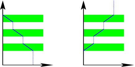
Figure 1: Construction of the function $v_{l}^{\eta}$, when $u^{\ast}(v_{l,j})<0$ (left) and $u^{\ast}(v_{l,j})>0$ (right). The set $E_{\eta}(v_{l,j})$ is coloured. The piecewise affine function $v_{l}^{\eta}$ is discontinuous, with derivative equal to $1/a<0$ (left) or $1/b>0$ (right). Notice that $v_{l}^{\eta}$ is injective in both cases. The derivative $u_{l}^{\eta}$ of the reciprocal function of $v_{l}^{\eta}$ is piecewise affine and takes value in $\{a,0,b\}$.

By construction, the function $v_{l}^{\eta}$ is one-to-one on $(t_{l,j},t_{l,j+1})$. Its inverse on $(t_{l,j},t_{l,j+1})$, say $w_{l}^{\eta}$, is a piecewise affine function. The derivative $u_{l}^{\eta}$ of the continuous piecewise linear function $w_{l}^{\eta}$ is a piecewise constant function taking value in $\{a,0,b\}$.

Moreover, by construction $\|u_{l}^{\eta}\|_{L^{1}}=\|u^{\ast}\|_{L^{1}}$.

For every $n$ in $\mathbf{N}$, let $u_{n}=u_{l}^{\eta}$ with $l=\eta=1/n$, let $v_{n}$ be the (possibly discontinuous) inverse function of $t\mapsto\int_{0}^{t}|u_{n}(s)|\mathrm{d}s$, and $y_{n}$ the associated solution of $\dot{y}=M_{u_{n}}y$ with initial condition $y(0)=I_{N}$.

For every $t$, $\int_{0}^{t}M_{u_{n}}(\tau)\mathrm{d}\tau$ tends to $\int_{0}^{t}M_{u^{\ast}}(\tau)\mathrm{d}\tau$ as $n$ tends to infinity, uniformly on $\left[0,\|u^{\ast}\|_{L^{1}}\right]$. By [6, Lemma 8.2], the associated solution $y_{n}$ tends uniformly on $[0,\|u^{\ast}\|_{L^{1}}]$ to $y^{\ast}$. In particular, $y_{n}(\|u^{\ast}\|_{L^{1}})$ converge toward $y^{\ast}(\|u^{\ast}\|_{L^{1}})$ as $n$ tends to infinity.

From (6), we have that for every $t$ in $[0,\|u^{\ast}\|_{L^{1}}]$,

$$\|X^{u^{\ast}}_{(N)}(v^{\ast}(t),0)-X^{u_{n}}_{(N)}(v_{n}(t),0)\|$$ (7)

$$\leq \|e^{v^{\ast}(t)A^{(N)}}y^{\ast}(t)-e^{v_{n}(t)A^{(N)}}y_{n}(t)\|$$

$$\leq \|y^{\ast}(t)-y_{n}(t)\|+\left\|e^{v^{\ast}(t)A^{(N)}}-e^{v_{n}(t)A^{(N)}}\right\|.$$

Taking $t=\|u^{\ast}\|_{L^{1}}$ in (7) concludes the first part of the proof.

Finally, notice that if $u^{\ast}\geq 0$, then $u^{\ast}(v_{l,j})$ is always nonnegative, hence $v_{\eta}^{\eta}$ is increasing and $u_{n}$ takes only the values $0$ and $b$. ∎

III INFINITE DIMENSIONAL SYSTEMS

III-A Energy estimates for weakly-coupled quantum systems

If $(A,B,C,k)$ satisfies Assumption 1, $(A,B,C)$ is $k$-weakly-coupled. We present here some properties of these systems and refer to [16] for further details.

The notion of weakly-coupled systems is closely related to the growth of the $k/2$-norm $\|\psi\|_{k/2}=\langle|A|^{k}\psi,\psi\rangle$. For $k=1$, this quantity is the expected value of the energy of the system. Next result is a direct application of [16, Proposition 2]

Proposition 8.

Let $(A,B,C,k)$ satisfy Assumption 1. Then, for every $\psi_{0}\in D(|A|^{k/2})$, $K>0$, $T\geq 0$, and $u$ piecewise constant such that $\|u\|_{L^{1}}+\|u\|^{2}_{L^{2}}<K$, one has

$$\left\|\Upsilon^{u}_{T}(\psi_{0})\right\|_{k/2}\leq e^{c(A,B,C,k)K}\|\psi_{0}\|_{k/2}.$$ (8)

Equation (8) allows to define the solutions of (2) for controls $u$ that are not necessarily piecewise constant. Indeed, let $u$ be in $L^{1}(\mathbf{R},\mathbf{R})\cap L^{2}(\mathbf{R},\mathbf{R})$ with support in $[0,T]$ for some $T>0$. There exists a sequence $(u_{n})_{n\in\mathbf{N}}$ of piecewise constant functions with support in $[0,T]$ such that $\|u_{n}\|_{L^{1}}\leq\|u\|_{L^{1}}$ and $\|u_{n}\|_{L^{2}}\leq\|u\|_{L^{2}}$ for every $n$ in $\mathbf{N}$ and the sequence $(u_{n})_{n\in\mathbf{N}}$ tends to $u$ both in $L^{1}$ and in $L^{2}$ norm. Next result then guarantees convergence of the propagators.

Lemma 9.

Let $(u_{n})_{n\in\mathbf{N}}$ be a Cauchy sequence of piecewise constant functions both in $L^{1}$ and $L^{2}$, then for every $t$ in $\mathbf{R}$ and every $\psi$ in $D(A)$, the sequence $(\Upsilon^{u_{n}}_{t,0}\psi)_{n\in\mathbf{N}}$ is a Cauchy sequence.

Proof.

For the sake of simplicity, we define $x_{n}:t\mapsto\Upsilon^{u_{n}}_{t,0}\psi$. Since $\psi$ belongs to the common domain $D(A)$ of the operators $D(A+\alpha B+\alpha^{2}C),$ for $\alpha\in\mathbf{R}$, the continuous mapping $x_{n}$ is a strong solution of (2), see [17]. Hence, $x_{n}$ is differentiable almost everywhere, $x_{n}(t)=x_{n}(0)+\int_{0}^{t}\dot{x}_{n}(s)\mathrm{d}s$ for every $t$ in $\mathbf{R}$ where $\dot{x}_{n}(t)=Ax_{n}(t)+u_{n}Bx_{n}(t)+u_{n}^{2}Cx_{n}(t)$ for almost every $t$ in $\mathbf{R}$.

Let $n,m$ in $\mathbf{N}$. The continuous mapping $x_{n}-x_{m}$ is differentiable almost everywhere and, for almost every $t$ in $\mathbf{R}$,

$$\frac{{d}}{{d}t}(x_{n}-x_{m})\big{|}_{t} \!=\!A(x_{n}-x_{m})(t)+(u_{n}(t)-u_{m}(t))Bx_{n}(t)$$

$$\quad+u_{m}(t)B(x_{n}(t)-x_{m}(t))$$

$$\quad+(u_{n}^{2}(t)-u_{m}^{2}(t))Cx_{n}(t)$$

$$\quad+u_{m}^{2}(t)C(x_{n}(t)-x_{m}(t))$$

By Duhamel formula, for every $t$ in $\mathbf{R}$,

$$\|(x_{n}-x_{m})(t)\|= \big{\|}\int_{0}^{t}\Upsilon^{u_{m}}_{t,s}(u_{n}(s)-u_{m}(s))Bx_{n}(s)$$

$$\quad+(u_{n}^{2}-u_{m}^{2})(s)Cx_{n}(s))\mathrm{d}s\big{\|}$$

$$\leq \|u_{n}-u_{m}\|_{L^{1}}\sup_{s\in\mathbf{R}}\|Bx_{n}(s)\|$$

$$\quad+\|u_{n}^{2}-u_{m}^{2}\|_{L^{1}}\sup_{s\in\mathbf{R}}\|Cx_{n}(s)\|$$ (9)

By Proposition 8, if $\|u\|_{L^{1}}+\|u\|^{2}_{L^{2}}<K$ then

$$\sup_{s\in\mathbf{R}}\||A|^{\frac{k}{2}}x_{n}(s)\|\leq e^{c(A,B,C,k)K}\||A|^{\frac{k}{2}}\psi\|.$$

Notice, and this is crucial for the result, that the RHS does not depend on $n$. By Assumption 1.5, $\sup_{n\in\mathbf{N}}\sup_{s\in\mathbf{R}}\|Bx_{n}(s)\|<+\infty$ and $\sup_{n\in\mathbf{N}}\sup_{s\in\mathbf{R}}\|Cx_{n}(s)\|<+\infty$.

Since $(u_{n})_{n\in\mathbf{N}}$ is a Cauchy sequence for the norms $L^{1}$ and $L^{2}$ then $\lim_{N\to\infty}\sup_{n,m\geq N}\|u_{n}-u_{m}\|_{L^{1}}=0$ and

$$\lim_{N\to\infty}\sup_{n,m\geq N}\|u_{n}^{2}-u_{m}^{2}\|_{L^{1}}$$

$$\leq \lim_{N\to\infty}\sup_{n,m\geq N}\|u_{n}-u_{m}\|_{L^{2}}\|u_{n}+u_{m}\|_{L^{2}}$$

$$\leq 2\lim_{N\to\infty}\sup_{n,m\geq N}\|u\|_{L^{2}}\|u_{n}-u_{m}\|_{L^{2}}=0,$$

hence, by (9) we have $\lim_{N\to\infty}\sup_{n,m\geq N}\|x_{n}(t)-x_{m}(t)\|=0$. ∎

Thanks to Lemma 9 and to the completeness of the Hilbert space $H$, one can define $\Upsilon^{u}_{t,0}\psi$ for $\psi$ in $D(A)$ as the limit of $\Upsilon^{u_{n}}_{t,0}\psi$ as $n$ tends to infinity. Notice that this limit is independent on the chosen approaching sequence $(u_{n})_{n\in\mathbf{N}}$ . For every $t\geq 0$, the mapping $\psi\mapsto\Upsilon^{u}_{t,0}\psi$ admits a unique unitary extension on $H$. We can therefore define the propagator associated with a control $u$ which is both $L^{1}$ and $L^{2}$, as summed up in the following result.

Proposition 10.

Let $(A,B,C,k)$ satisfy Assumption 1. The mapping $u\mapsto\Upsilon_{\cdot,0}^{u,(A,B,C)}$ which associates with every piecewise constant function a continuous curve of unitary transformations of $H$ bounded for the $\|\cdot\|_{k}$ norm admits a unique continuous extension for the $\|\cdot\|_{L^{1}}+\|\cdot\|_{L^{2}}$-norm.

Thanks to Proposition 10, one can extend the result of Proposition 8 to functions in $L^{1}(\mathbf{R})\cap L^{2}(\mathbf{R})$. Another application (instrumental in our study) of Proposition 8 is the following approximation result, based on [16, Theorem 4].

Proposition 11.

Let $k$ in $\mathbf{N}$ and $(A,B,C,k)$ satisfy Assumption 1. Then for every $\varepsilon>0$, $s<k$, $K\geq 0$, $n\in\mathbf{N}$, and $(\psi_{j})_{1\leq j\leq n}$ in $D(|A|^{k/2})^{n}$ there exists $N\in\mathbf{N}$ such that for every piecewise constant function $u$ we have that

$$\|u\|_{L^{1}}+\|u\|^{2}_{L^{2}}<K\Rightarrow\|\Upsilon^{u}_{t}(\psi_{j})-X^{u}_{(N)}(t,0)\pi_{N}\psi_{j}\|_{s/2}<\varepsilon,$$

for every $t\geq 0$ and $j=1,\ldots,n$.

Proof.

The result for $u$ piecewise constant is given by [16, Theorem 4]. Then, by density, (see Proposition 10), the result holds true for general $u$ in $L^{1}(\mathbf{R},\mathbf{R})\cap L^{2}(\mathbf{R},\mathbf{R})$. ∎

Remark 3.

In Propositions 8 and 11, the upper bound of the $|A|^{k/2}$ norm of the solution of (2) or the bound on the error between the infinite dimensional system and its finite dimensional approximation only depend on the $L^{1}$ and $L^{2}$ norms of the control, not on the time.

III-B An infinite dimensional tracking result

Proposition 11 allows to adapt finite dimensional results to infinite dimensional systems. Here we present a sort of “Bang-Bang” Theorem for infinite dimensional systems.

Lemma 12.

Let $(A,B,0,k)$ satisfy Assumption 1 with $k$ in $\mathbf{N}$, $T$ be a positive number, $a,b$ be two real numbers such that $a<0<b$, $u^{\ast}$ be a locally integrable function with support in $[0,T]$, and $N$ be an integer. Then, for every $\varepsilon>0$, there exists a piecewise constant control $u_{\varepsilon}:[0,T_{\varepsilon}]\to\{a,0,b\}$ such that, for every $j\leq N$, $\|{\Upsilon^{u_{\varepsilon}}_{T_{\varepsilon},0}(\phi_{j})-\Upsilon^{u^{\ast}}_{T,0}(\phi_{j})}\|<\varepsilon$, and $\|u_{\varepsilon}\|_{L^{1}}\leq\|u^{\ast}\|_{L^{1}}$. Moreover, if $u^{\ast}$ is positive, then $u_{\varepsilon}$ may be chosen with value in $\{0,b\}$.

Proof.

Let $\varepsilon>0$. By Proposition 11, there exists $N$ in $\mathbf{N}$ such that, for every piecewise constant function $u$ and for every $j\leq N$,

$$\|u\|_{L^{1}}\leq\|u^{\ast}\|_{L^{1}}\Rightarrow\|\Upsilon^{u}_{t}(\phi_{j})-X^{u}_{(N)}(t,0)\pi_{N}\phi_{j}\|<\varepsilon.$$

From Lemma 7, there exists $u_{\varepsilon}:[0,T\varepsilon]\rightarrow\{a,0,b\}$ piecewise constant such that $\|u_{\varepsilon}\|_{L^{1}}\leq\|u^{\ast}\|_{L^{1}}$ and

$$\|X^{u^{\ast}}_{(N)}(T,0)-X^{u_{\varepsilon}}_{(N)}(T,0)\|<\varepsilon.$$

Then, for every $j\leq N$,

$$\|\Upsilon^{u_{\varepsilon}}_{T_{\varepsilon},0}(\phi_{j})-\Upsilon^{u^{\ast}}_{T,0}(\phi_{j})\|$$

$$\leq \|\Upsilon^{u_{\varepsilon}}_{T_{\varepsilon},0}(\phi_{j})-X^{u_{\varepsilon}}_{(N)}(t,0)\pi_{N}\phi_{j}\|$$

$$+\|X^{u_{\varepsilon}}_{(N)}(T_{\varepsilon},0)\pi_{N}\phi_{j}-X^{u^{\ast}}_{(N)}(T,0)\pi_{N}\phi_{j}\|$$

$$+\|\Upsilon^{u^{\ast}}_{T,0}(\phi_{j})-X^{u^{\ast}}_{(N)}(T,0)\pi_{N}\phi_{j}\|$$

$$\leq 3\varepsilon.$$

The same proof shows that, if $u^{\ast}$ is positive, $u_{\varepsilon}$ can be chosen with values in $\{0,b\}$. ∎

III-C Simultaneous approximate controllability

We recall here the following result dealing with approximate controllability for bilinear systems, i.e. when $C=0$. Its proofs is given in [8, Theorem 2.11].

Theorem 13 ([8]).

Let $(A,B,0,0)$ satisfy Assumption 1. If there exists a non-resonant chain of connectedness of $(A,B,0)$ then, for every $N$ in $\mathbf{N}$, for every $\varepsilon>0$, for every $\delta>0$, for every unitary operator $\hat{\Upsilon}:H\to H$, there exists $T>0$ and a piecewise constant function $u:[0,T]\rightarrow[0,\delta]$ such that $\|\Upsilon^{u}_{T,0}\phi_{j}-\hat{\Upsilon}\phi_{j}\|<\varepsilon$, for every $j\leq N$.

We now proceed to the proof of the Theorem 2.

Proof of Theorem 2 (case $r=0$).

Assume that $(A,B,C,k)$ satisfies Assumption 1 for some $k$ in $\mathbf{N}$ and admits a strongly non-degenerate chain of connectedness. Then, there exists $\alpha>0$ such that $(A,B+\alpha C,0)$ satisfies Assumption 1 and admits a strongly non-degenerate chain of connectedness. By analyticity, this property is true for almost every $\alpha$ in $\mathbf{R}$. From Theorem 13, for every $N$ in $\mathbf{N}$, for every unitary operator $\hat{\Upsilon}:H\to H$ for every $\varepsilon>0$, and for every $\delta>0$, there exist $T>0$ and a piecewise constant function $u:[0,T]\rightarrow[0,\delta]$ such that $\|\Upsilon^{u,(A,B+\alpha C,0)}_{T,0}\phi_{j}-\hat{\Upsilon}\phi_{j}\|<\varepsilon$. By Lemma 12, there exists $\tilde{u}:[0,T_{\tilde{u}}]\rightarrow\{0,\alpha\}$ such that $\|\Upsilon^{\tilde{u},(A,B+\alpha C,0)}_{T_{\tilde{u}},0}\phi_{j}-\Upsilon^{u,(A,B+\alpha C,0)}_{T,0}\phi_{j}\|<\varepsilon$. Thus, for $j\leq N$, $\|\Upsilon^{\tilde{u},(A,B+\alpha C,0)}_{T_{\tilde{u}},0}\phi_{j}-\hat{\Upsilon}\phi_{j}\|<2\varepsilon$. To conclude the proof of Theorem 2 for $r=0$, it is enough to notice that $\Upsilon^{\tilde{u},(A,B+\alpha C,0)}_{T_{\tilde{u}},0}=\Upsilon^{\tilde{u},(A,B,C)}_{T_{\tilde{u}},0}$, since for every $t$, $\tilde{u}(t)B+\tilde{u}^{2}(t)C=\tilde{u}(t)(B+\alpha C)$ as $\tilde{u}$ takes only the values $0$ and $\alpha$. ∎

III-D Controllability between eigenstates

In this Section, we use averaging techniques to provide explicit expressions of control laws steering one eigenstate of the system to another in order to prove Theorems 3 and 4.

Averaging methods consist in replacing an oscillating dynamics $\dot{y}=f(t)y$ by its average $\dot{z}=\bar{f}z$ where $\bar{f}=\lim\frac{1}{T}\int_{0}^{T}f(t)\mathrm{d}t$. When the dynamics $f$ is regular and small enough, the solutions $y$ and $z$ have similar behaviors. Averaging theory has grown to a whole theory in itself. We refer to [18] for an introduction. In quantum mechanics, averaging theory has been extensively used (under the name of “Rotating Wave Approximation”) since the 60’s, for finite dimensional systems. It has recently been extended to the case of infinite dimensional systems. In the following proposition, we restate [12, Theorem 1 and Section 2.4] in our framework.

Proposition 14.

Let $(A,B,0,k)$ satisfy Assumption 1. Assume that $(p,q)$ is a weakly non-degenerate transition of $(A,B,0)$. Define $\mathcal{N}=\{n\in\mathbf{N}\,|\,$ there exists $(l_{1},l_{2})\mbox{ with }b_{l_{1},l_{2}}\neq 0\mbox{ and }|l_{1}-l_{2}|=n|\lambda_{p}-\lambda_{q}|\mbox{ and }\{l_{1},l_{2}\}\cap\{p,q\}\neq\emptyset\}.$ If $u$ and $u^{2}$ are locally integrable, $2\pi/|\lambda_{p}-\lambda_{q}|$-periodic and satisfies, for every $n$ in $\mathcal{N}$,

$$\int_{0}^{2\pi/|\lambda_{p}-\lambda_{q}|}\!\!\!\!\!\!\!\!e^{\mathrm{i}n|\lambda_{p}-\lambda_{q}|t}u(t)\mathrm{d}t\neq 0\quad\mbox{ if }n=1$$ (10)

and

$$\int_{0}^{2\pi/|\lambda_{p}-\lambda_{q}|}\!\!\!\!\!\!\!\!e^{\mathrm{i}n|\lambda_{p}-\lambda_{q}|t}u(t)\mathrm{d}t=0\quad\mbox{ if }n>1$$ (11)

then there exists $T^{\ast}>0$ such that $|\langle\phi_{p},\Upsilon^{u^{\ast}/n,(A,B,0)}_{nT^{\ast},0}\phi_{q}\rangle|$ tends to $1$ as $n$ tends to infinity. Moreover,

$$\lim_{n\to\infty}\frac{1}{n}\int_{0}^{nT^{\ast}}|u^{\ast}(t)|\mathrm{d}t\leq\frac{\pi}{2|b_{pq}|}\frac{\int_{0}^{T}|u^{\ast}(t)|\mathrm{d}t}{\left|\int_{0}^{T}u^{\ast}(t)\mathrm{d}t\right|}.$$

Our aim is to extend the result of Proposition 14 to the case where $C\neq 0$.

Proposition 15.

Let $(A,B,C,k)$ satisfy Assumption 1. Assume that $(p,q)$ is a weakly non-degenerate transition of $(A,B,0)$. Define $\mathcal{N}=\{n\in\mathbf{N}\,|\,$ there exists $(l_{1},l_{2})\mbox{ with }b_{l_{1},l_{2}}\neq 0\mbox{ and }|l_{1}-l_{2}|=n|\lambda_{p}-\lambda_{q}|\mbox{ and }\{l_{1},l_{2}\}\cap\{p,q\}\neq\emptyset\}.$ If $u$ and $u^{2}$ are locally integrable, $2\pi/|\lambda_{p}-\lambda_{q}|$-periodic and satisfy, for every $n$ in $\mathcal{N}$,

$$\int_{0}^{2\pi/|\lambda_{p}-\lambda_{q}|}\!\!\!\!\!\!\!\!e^{\mathrm{i}n|\lambda_{p}-\lambda_{q}|t}u(t)\mathrm{d}t\neq 0\quad\mbox{ if }n=1$$

and

$$\int_{0}^{2\pi/|\lambda_{p}-\lambda_{q}|}\!\!\!\!\!\!\!\!e^{\mathrm{i}n|\lambda_{p}-\lambda_{q}|t}u(t)\mathrm{d}t=0\quad\mbox{ if }n>1$$

then there exists $T^{\ast}>0$ such that $|\langle\phi_{p},\Upsilon^{u^{\ast}/n,(A,B,C)}_{nT^{\ast},0}\phi_{q}\rangle|$ tends to $1$ as $n$ tends to infinity.

Proof.

For the sake of readability, we define $T:=\frac{2\pi}{|\lambda_{p}-\lambda_{q}|}$. Let $u$ be a locally integrable and square integrable $T$-periodic function satisfying (10) and (11). By Proposition 14 there exists $T^{*}>0$ such that $|\langle\phi_{p},\Upsilon^{u^{\ast}/n,(A,B,0)}_{nT^{\ast},0}\phi_{q}\rangle|\to 1$ as $n\to+\infty$.

Notice that, for every $n$ in $\mathbf{N}$,

$$\int_{0}^{nT^{\ast}}\left|\frac{u(s)}{n}\right|^{2}\mathrm{d}s \leq \frac{1}{n^{2}}\left(\frac{nT^{\ast}}{T}+1\right)\int_{0}^{T}\!\!\!|u(s)|^{2}\mathrm{d}s$$ (12)

$$= \left(\frac{T^{\ast}}{nT}+\frac{1}{n^{2}}\right)\int_{0}^{T}\!\!\!|u(s)|^{2}\mathrm{d}s.$$

By Proposition 8,

$$\sup_{n\in\mathbf{N}}\sup_{0\leq s,t\leq nT^{\ast}}\|\Upsilon^{u/n,(A,B,C)}_{s,t}\phi_{q}\|_{k/2}<+\infty,$$ (13)

and, by Assumption 1.5,

$$\sup_{n\in\mathbf{N}}\sup_{0\leq s,t\leq nT^{\ast}}\|C\Upsilon^{u/n,(A,B,C)}_{s,t}\phi_{q}\|<+\infty.$$ (14)

Since $\phi_{q}$ belongs to $D(A)$, for every $n$ in $\mathbf{N}$ the mapping $t\mapsto\Upsilon^{u/n,(A,B,C)}_{t,0}\phi_{q}$ is a strong solution of (2). For every $n\in\mathbf{N}$, by Duhamel formula we have,

$$\left\|\Upsilon^{u/n,(A,B,C)}_{nT^{\ast},0}\phi_{q}-\Upsilon^{u/n,(A,B,0)}_{nT^{\ast},0}\phi_{q}\right\|$$

$$= \left\|\frac{1}{n^{2}}\int_{0}^{nT^{\ast}}\!\!\!\!\!\!\!\!\!\!u^{2}(s)\Upsilon^{u/n,(A,B,0)}_{nT^{\ast},s}C\Upsilon^{u/n,(A,B,C)}_{s,0}\phi_{q}\mathrm{d}s\right\|$$

$$\leq \left(\frac{1}{n^{2}}\int_{0}^{nT^{\ast}}\!\!\!\!\!\!\!\!\!\!u^{2}(s)\mathrm{d}s\right)\sup_{n\in\mathbf{N}}\sup_{0\leq s,t\leq nT^{\ast}}\|C\Upsilon^{u/n,(A,B,C)}_{s,t}\phi_{q}\|$$

From (12) and (14), this last quantity tends to zero as $n$ tends to infinity, and Proposition 15 follows from Proposition 14. ∎

We now proceed to the proofs of Theorems 3 and Theorems 4 in the case $r=0$.

Proof of Theorem 4 (case $r=0$).

Let $\varepsilon>0$ and $\delta>0$ such that $b_{pq}+\delta c_{pq}\neq 0$ be given and define $T=2\pi/|\lambda_{p}-\lambda_{q}|$. Using $u^{\ast}:t\mapsto 1+\sin(t2\pi/T)$ with the system $(A,B+\delta C,0)$, Proposition 14 states that there exists $T^{\ast}$ such that $|\langle\phi_{p},\Upsilon^{u^{\ast}/n,(A,B+\delta C,0)}_{nT^{\ast},0}\phi_{q}\rangle|$ tends to $1$ as $n$ tends to infinity.

By Assumption 1, the real number $\lambda_{p}$ is not zero. Hence there exists a sequence $(t_{n})_{n\in\mathbf{N}}$ such that $\|e^{t_{n}A}\Upsilon^{u^{\ast}/n,(A,B+\delta C,0)}_{nT^{\ast},0}\phi_{q}-\phi_{p}\|$ tends to zero as $n$ tends to infinity. Notice that

$$e^{t_{n}A}\Upsilon^{u^{\ast}/n,(A,B+\delta C,0)}_{nT^{\ast},0}\phi_{q}=\Upsilon^{w_{n},(A,B+\delta C,0)}_{nT^{\ast}+t_{n},0}\phi_{q},$$

where $w_{n}(s)=u^{\ast}(s)/n$ for $s\leq nT^{\ast}$ and $w_{n}(s)=0$ for $s\in(nT^{\ast},nT^{\ast}+t_{n})$.

From Lemma 12, for every $n$ in $\mathbf{N}$, there exists $u_{n}:[0,T_{n}]\to\{0,\delta\}$ such that $\|\Upsilon^{u_{n},(A,B+\delta C,0)}_{T_{n},0}\phi_{q}-\Upsilon^{w_{n},(A,B+\delta C,0)}_{nT^{\ast}+t_{n},0}\phi_{q}\|<\varepsilon$. Conclusion follows from the fact that $\Upsilon^{u_{n},(A,B+\delta C,0)}_{T_{n},0}\phi_{q}=\Upsilon^{u_{n},(A,B,C)}_{T_{n},0}\phi_{q}$, for every $n$ in $\mathbf{N}$. ∎

While primary oriented to the non-bilinear system (2), Theorem 4 holds when $C=0$ and represents a slight improvement (by a factor $4/5$) of Proposition 2.8 in [8].

Proof of Theorem 3 (case $r=0$).

Let $S$ be a weakly-non-degenerate chain of connectedness of $(A,B,C)$. Theorem 3 for $r=0$ is a consequence Theorem 4 applied iteratively on every pair $(p,q)$ in $S$. ∎

III-E Approximate controllability in higher norms

The proofs of Theorems 3 and 4 for the general case $r>0$ are a consequence of an easy and well-known result of interpolation. We give a proof for the sake of completeness.

Lemma 16.

Let $s<r$ be two real numbers, $(x_{n})_{n\in\mathbf{N}}$ be a sequence that converges to zero in $H$ in $s$-norm and is bounded in $r$-norm. Then $(x_{n})_{n\in\mathbf{N}}$ tends to zero in $q$-norm for any $q<r$.

Proof.

We first prove the result for $q<(r+s)/2$. For every $n$ in $\mathbf{N}$,

$$\|x_{n}\|_{\frac{s+r}{2}}^{2} = \langle|A|^{\frac{s+r}{2}}x_{n},|A|^{\frac{s+r}{2}}x_{n}\rangle$$

$$= \langle|A|^{s}x_{n},|A|^{r}x_{n}\rangle$$

$$\leq \|x_{n}\|_{s}\sup_{n\in\mathbf{N}}\|x_{n}\|_{r},$$

which tends to zero as $n$ tends to infinity. Replacing $s$ in the computation above by $(s+r)/2$ gives the result for $q<r-(r-s)/4$. After $N$ iterations of this process, the result is proved for any $q$ less than $r-(r-s)/2^{N}$ which tends to $r$ as $N$ tends to infinity. ∎

The general proof of the main results for the general case $r>0$ is then a consequence of this interpolation lemma, of Proposition 8, and of the uniform bound on the $L^{1}$ and $L^{2}$ norm of the controls. Notice that the bound on the square of the $L^{2}$ norm of the control taking value in $\{0,\delta\}$ is exactly $\delta$ times the $L^{1}$ norm, since, for every $\delta$ in $\mathbf{R}$, $u^{2}=\delta u$ if $u\in\{0,\delta\}$. The three proof follows exactly the same strategy.

Proof of Theorem 2.

The sequence of propagators $\Upsilon^{u_{\varepsilon}}_{T_{\varepsilon},0}\phi_{j}$ tends to $\hat{\Upsilon}\phi_{j}$ in the norm of $H$. The sequence of controls $u_{\varepsilon}$ is bounded in the $L^{1}$ norm by [8, Remark 5.9], then we can apply Proposition 8 to have a bound on the $k/2$-norm. The result then follows from Lemma 16. ∎

Proof of Theorem 4.

The proof follows the proof of Theorem 2 above. We prove that there exists a sequence of controls $u_{\varepsilon}:[0,T_{\varepsilon}]\rightarrow\{0,\delta\}$ such that $\|u_{\varepsilon}\|_{L^{1}}\leq\pi/(|b_{pq}+\delta c_{pq})$ and $\|\Upsilon^{u_{\varepsilon}}_{T_{\varepsilon},0}\phi_{p}-\phi_{q}\|$ tends to $0$ as $\varepsilon$ tends to $0$. Moreover the sequence $\Upsilon^{u_{\varepsilon}}_{T_{\varepsilon},0}\phi_{p}$ is bounded for the $k/2$-norm by Proposition 8 and Lemma 16 allows to conclude that $\|\Upsilon^{u_{\varepsilon}}_{T_{\varepsilon},0}\phi_{p}-\phi_{q}\|_{r}$ tends to $0$ as $\varepsilon$ tends to $0$ for every $r<k/2$. ∎

Proof of Theorem 3.

It is sufficient to notice that the bound on $L^{1}$-norm of the sequence of controls $u_{\varepsilon}$ is given by iteratively apply Theorem 4 to every element of the connectedness chain connecting $p$ to $q$. The proof then follows from Proposition 8 and Lemma 16 as in the proof of Theorems 2 and 4. ∎

IV EXAMPLES

IV-A Bounded coupling potentials

Let $\Omega$ be a compact Riemannian manifold or a bounded domain in $\mathbf{R}^{n}$. Let $V,W_{1},W_{2}:\Omega\to\mathbf{R}$ be three measurable bounded functions. We consider the system

$$\mathrm{i}\frac{\partial\psi}{\partial t}(x,t)=(-\Delta+V(x))\psi(x,t)+u(t)W_{1}(x)\psi(x,t)$$ (15)

$$\quad\quad\quad\quad\quad\quad\quad\quad\quad+u^{2}(t)W_{2}(x)\psi(x,t),\quad\quad$$

with $x$ in $\Omega$ and $t$ in $\mathbf{R}$. This system has been studied in [5] when $\Omega$ is a bounded domain of $\mathbf{R}^{n}$, and the potentials $W_{1}$ and $W_{2}$ are $C^{2}$.

In order to apply our results, we define $H=L^{2}(\Omega,\mathbf{C})$, $A:\psi\in D(A)\mapsto\mathrm{i}(\Delta-V)\psi$, $B:\psi\in L^{2}(\Omega,\mathbf{C})\mapsto-\mathrm{i}W_{1}\psi$ and $C:\psi\in L^{2}(\Omega,\mathbf{C})\mapsto-\mathrm{i}W_{2}\psi$. By Kato-Rellich theorem, the domain $D(A)$ of $A$ is equal to $H^{2}_{(0)}=\{\psi\in H^{2}(\Omega,\mathbf{C})|\psi_{|\partial\Omega}=\Delta\psi_{|\partial\Omega}=0\}$, the domain of the Laplacian, if $\Omega$ is a bounded domain of $\mathbf{R}^{n}$ and equal to $H^{2}(\Omega,\mathbf{C})$ if $\Omega$ is compact manifold. The operators $B$ and $C$ are bounded from $H$ to $H$ with norms $\|W_{1}\|_{L^{\infty}}$ and $\|W_{2}\|_{L^{\infty}}$, respectively.

We restrict ourselves to the generic case (see [19]) where $A$ has only simple eigenvalues. Without further regularity assumptions on $W_{1}$ and $W_{2}$, it is not clear if $(A,B,C,k)$ satisfies Assumption 1 for any $k>0$.

By standard regularization procedures for every $\eta>0$, there exist $W_{1,\eta},W_{2,\eta}:\Omega\to\mathbf{R}$ such that (i) $W_{1,\eta}$ $W_{2,\eta}$ are $C^{2}$ on $\Omega$, (ii) if $\Omega$ is a bounded domain of $\mathbf{R}^{n}$, $W_{1,\eta}$ and $W_{2,\eta}$ tend to zero, with their two first derivatives, on the boundary of $\Omega$, and (iii) $\|W_{j}-W_{j,\eta}\|_{L^{1}}\leq\eta$ for $j=1,2$. The linear operators $B_{\eta}:\psi\mapsto W_{1,\eta}\psi$ and $C_{\eta}:\psi\mapsto W_{2,\eta}\psi$ are bounded from $D(A)$ to $D(A)$. By Proposition 8 of [16], $(A,B_{\eta},C_{\eta})$ is $1$-weakly-coupled or, equivalently, $(A,B_{\eta},C_{\eta},1)$ satisfies Assumption 1.

Remark 4.

The definition of $\Upsilon^{u,(A,B_{\eta},C_{\eta})}$ depends on the choice of $B_{\eta}$ and $C_{\eta}$, which is not unique.

The key point of this section is the following observation.

Lemma 17.

For every $\eta>0$, for every $u$ in $L^{1}(\mathbf{R},\mathbf{R})\cap L^{2}(\mathbf{R},\mathbf{R})$, for every $t$ in $\mathbf{R}$, for every $\psi$ in $H$,

$$\|\Upsilon^{u,(A,B,C)}_{t,0}-\Upsilon^{u,(A,B_{\eta},C_{\eta})}_{t,0}\|\leq\eta(\|u\|_{L^{1}}+\|u\|_{L^{2}}^{2}).$$

Thanks to Lemma 17, we can apply the results above to system (15). For instance Theorem 2 applied to system (15) reads.

Proposition 18.

Assume that $(A,B,C)$ admits a strongly non-degenerate chain of connectedness. Then, for every $\varepsilon>0$, for every unitary $\hat{\Upsilon}:H\to H$, for every $l$ in $\mathbf{N}$, for almost every $\alpha>0$ there exists a piecewise constant function $u_{\varepsilon}:[0,T_{\varepsilon}]\to\{0,\alpha\}$ such that $\|\Upsilon^{u_{\varepsilon}}_{T_{\varepsilon},0}\phi_{j}-\hat{\Upsilon}\phi_{j}\|<\varepsilon$, for every $j\leq l$.

Proof.

For every $\alpha>0$ such that $S$ is a strongly non-degenerate chain of connectedness of $(A,B+\alpha C,0)$, by Theorem 13, there exists a piecewise constant function $u:[0,T]\to[0,\alpha]$ such that $\|\Upsilon^{u,(A,B+\alpha C,0)}_{T,0}\phi_{j}-\hat{\Upsilon}\phi_{j}\|<\varepsilon/3$, for every $j\leq l$. Define

$$\eta=\frac{1}{3}\frac{\varepsilon}{\|u\|_{L^{1}}(1+\alpha)}.$$

As before choose $W_{1,\eta},W_{2,\eta}:\Omega\to\mathbf{R}$ such that (i) $W_{1,\eta}$ $W_{2,\eta}$ are $C^{2}$ on $\Omega$, (ii) if $\Omega$ is a bounded domain of $\mathbf{R}^{n}$, $W_{1,\eta}$ and $W_{2,\eta}$ tend to zero, with their two first derivatives, on the boundary of $\Omega$, and (iii) $\|W_{j}-W_{j,\eta}\|_{L^{1}}\leq\eta$ for $j=1,2$. Then the linear operators $B_{\eta}:\psi\mapsto W_{1,\eta}\psi$ and $C_{\eta}:\psi\mapsto W_{2,\eta}\psi$ satisfy $\|B-B_{\eta}\|<\eta$, $\|C-C_{\eta}\|<\eta$ and $(A,B_{\eta},C_{\eta},1)$ satisfies Assumption 1.

By Lemma 12, there exists a piecewise constant function $u_{\varepsilon}:[0,T_{\varepsilon}]\to\{0,\alpha\}$ such that $\|u_{\varepsilon}\|_{L^{1}}\leq\|u\|_{L^{1}}$ and $\|\Upsilon^{u_{\varepsilon},(A,B_{\eta}+\alpha C_{\eta},0)}_{T_{\varepsilon},0}\phi_{j}-\Upsilon^{u,(A,B_{\eta}+\alpha C_{\eta},0)}_{T,0}\phi_{j}\|<\varepsilon/3$, for every $j\leq l$.

Notice that

$$\Upsilon^{u_{\varepsilon},(A,B_{\eta}+\alpha C_{\eta},0)}_{T_{\varepsilon},0}=\Upsilon^{u_{\varepsilon},(A,B_{\eta},C_{\eta})}_{T_{\varepsilon},0},$$

and $\|u_{\varepsilon}\|_{L^{2}}^{2}=\alpha\|u_{\varepsilon}\|_{L^{1}}$ since $u_{\varepsilon}$ takes value in $\{0,\alpha\}$.

Finally, for every $j\leq l$,

$$\|\Upsilon^{u_{\varepsilon},(A,B,C)}_{T_{\varepsilon},0}\phi_{j}-\hat{\Upsilon}\phi_{j}\|$$ (16)

$$\leq \|\Upsilon^{u_{\varepsilon},(A,B,C)}_{T_{\varepsilon},0}\phi_{j}-\Upsilon^{u_{\varepsilon},(A,B_{\eta},C_{\eta})}_{T_{\varepsilon},0}\phi_{j}\|$$

$$\quad+\|\Upsilon^{u_{\varepsilon},(A,B_{\eta},C_{\eta})}_{T_{\varepsilon},0}\phi_{j}-\Upsilon^{u_{\varepsilon},(A,B_{\eta}+\alpha C_{\eta},0)}_{T_{\varepsilon},0}\phi_{j}\|$$

$$\quad+\|\Upsilon^{u_{\varepsilon},(A,B_{\eta}+\alpha C_{\eta},0)}_{T_{\varepsilon},0}\phi_{j}-\Upsilon^{u,(A,B_{\eta}+\alpha C_{\eta},0)}_{T,0}\phi_{j}\|$$

$$\quad+\|\Upsilon^{u,(A,B_{\eta}+\alpha C_{\eta},0)}_{T,0}\phi_{j}-\hat{\Upsilon}\phi_{j}\|$$

$$\leq \frac{\varepsilon}{3}+0+\frac{\varepsilon}{3}+\frac{\varepsilon}{3}=\varepsilon.$$ (17)

Proposition 18 follows by observing that $S$ is a strongly non-degenerate chain of connectedness of $(A,B+\alpha C,0)$ for almost every $\alpha$ in $\mathbf{R}$, see Lemma 1. ∎

IV-B Perturbation of the harmonic oscillator

The quantum harmonic oscillator is among the most important examples of quantum system (see, for instance, [10, Complement $G_{V}$]). Its controlled bilinear version has been extensively studied (see, for instance, [20, 21] and references therein).

We consider here a 1D-model involving, in addition to the standard bilinear term modeling a constant electric field, a Gaussian perturbation. Precisely, for given constant $a>0,b$, and $c$, the dynamics is given, for $x$ in $\mathbf{R}$, by:

$$\mathrm{i}\frac{\partial\psi}{\partial t}=(-\Delta+x^{2})\psi+u(t)x\psi+u^{2}(t)e^{-ax^{2}+bx+c}\psi$$ (18)

With the notations of Section I-B we have $H=L^{2}(\mathbf{R},\mathbf{C})$, $A:\psi\mapsto\mathrm{i}(\Delta-x^{2})\psi$, $B:\psi\mapsto-\mathrm{i}x\psi$ and $C:\psi\mapsto-\mathrm{i}e^{-ax^{2}+bx+c}\psi$

A Hilbert basis of $H$ made of eigenvectors of $A$ is given by the sequence of the Hermite functions $(\phi_{n})_{n\in\mathbf{N}}$, associated with the sequence $(-\mathrm{i}\lambda_{n})_{n\in\mathbf{N}}$ of eigenvalues where $\lambda_{n}=n-1/2$ for every $n$ in $\mathbf{N}$. In the basis $(\phi_{n})_{n\in\mathbf{N}}$, $B$ admits a tri-diagonal structure

$$\langle\phi_{j},B\phi_{k}\rangle=\left\{\begin{array}[]{cl}-\mathrm{i}\sqrt{\frac{k}{2}}&\mbox{if }j=k-1,\\ -\mathrm{i}\sqrt{\frac{k+1}{2}}&\mbox{if }j=k+1,\\ 0&\mbox{otherwise.}\end{array}\right.$$

The operator $C$ couples most of the energy levels of $A$, see [7, Proposition 6.4].

For every $k$ in $\mathbf{N}$, the system $(A,B,0,k)$ satisfies Assumption 1 (see Section IV.E in [16]) and

$$c_{k}(A,B,0) \leq 3^{k}-1.$$

For every $k$ in $\mathbf{N}$, a direct computation shows that $C$ is bounded from $D(|A|^{k})$ to $D(|A|^{k})$. Hence, by Proposition 6 of [16], $(A,0,C,k)$ satisfies Assumption 1 for every $k$. Finally, $(A,B,C,k)$ satisfies Assumption 1 for every $k$.

The quantum harmonic oscillator $(A,B,0)$ is not controllable (in any reasonable sense) as proved in [20]. We aim at proving the following.

Proposition 19.

Assume that $\sqrt{1-a}$ and $b$ are algebraically independent. Then, for every $\varepsilon>0$, for every $j$ in $\mathbf{N}$, there exist $T>0$ and a piecewise constant function $u:[0,T]\to\mathbf{R}$ such that $\|\Upsilon^{u}_{T,0}\phi_{1}-\phi_{j}\|<\varepsilon$.

The main tool in the proof of Proposition 19 is the following analytic perturbation argument (see Chapter VII of [22]).

Proposition 20 ([22]).

For every $\alpha$ in $\mathbf{R}$ and $n$ in $\mathbf{N}$, there exist two analytic mappings $\boldsymbol{\lambda}^{\alpha}_{n}:\mathbf{R}\to\mathbf{R}$ and $\boldsymbol{\phi}^{\alpha}_{n}:\mathbf{R}\to L^{2}(\mathbf{R},\mathbf{C})$ such that (i) for every $t$ in $\mathbf{R}$, $A+t(B+\alpha C)\boldsymbol{\phi}^{\alpha}_{n}(t)=-\mathrm{i}\boldsymbol{\lambda}^{\alpha}_{n}(t)\boldsymbol{\phi}^{\alpha}_{n}(t)$; (ii) $\left.\frac{d}{dt}\boldsymbol{\lambda}^{\alpha}_{n}(t)\right|_{0}=b_{nn}+\alpha c_{nn}$; (iii) for every $t$ in $\mathbf{R}$, $(\boldsymbol{\phi}^{\alpha}_{n}(t))_{n\in\mathbf{N}}$ is a Hilbert basis of $L^{2}(\mathbf{R},\mathbf{C})$; (iv) $(\boldsymbol{\phi}^{\alpha}_{n}(0))_{n\in\mathbf{N}}=({\phi}_{n})_{n\in\mathbf{N}}$.

Proof of Proposition 19.

From Proposition 6.4 of [7], for every $n$ in $\mathbf{N}$, the pair $(n,n+1)$ is a strongly non-degenerate transition of $(A+\mu(B+2\alpha C),B+\alpha C,0)$ for almost every $(\alpha,\mu)$ in $\mathbf{R}^{2}$.

We proceed by induction. For $p=2$, choose $\alpha$ and $\mu$ positive small enough such that, with the notations of Proposition 20, $\|\boldsymbol{\phi}^{\alpha}_{j}(\mu)-\alpha_{j}\|<\varepsilon/4$ for $j=1,2$, $|b_{12}+\alpha c_{12}|=\left|1+\frac{\alpha be^{c-\frac{b^{2}}{4(a-1)}}}{\sqrt{2}(1-a)^{3/2}}\right|\neq 0$ and $\mu^{2}+2\mu+\mu\alpha<\frac{\varepsilon}{4\pi\|C\|}$ By Theorem 4, there exists a piecewise constant function $v:[0,T]\to[0,1]$ such that $\|\Upsilon^{v,(A+\mu(B+\alpha C),B,C)}_{T}\boldsymbol{\phi}^{\alpha}_{1}(\mu)-\boldsymbol{\phi}^{\alpha}_{2}(\mu)\|<\varepsilon/4$. Then, defining $u:t\in[0,T]\mapsto v(t)+\mu$:

$$\|\Upsilon^{u,(A,B,C)}_{T,0}\phi_{1}-\phi_{2}\|$$

$$\leq \|\Upsilon^{u,(A,B,C)}_{T,0}\phi_{1}-\Upsilon^{u,(A,B,C)}_{T,0}\boldsymbol{\phi}^{\alpha}_{1}(\mu)\|$$

$$\quad+\|\Upsilon^{u,(A,B,C)}_{T,0}\boldsymbol{\phi}^{\alpha}_{1}(\mu)-\Upsilon^{v,(A+\mu(B+\alpha C),B,C)}_{T,0}\boldsymbol{\phi}^{\alpha}_{1}(\mu)\|$$

$$\quad+\|\Upsilon^{v,(A+\mu(B+\alpha C),B,C)}_{T,0}\boldsymbol{\phi}^{\alpha}_{1}(\mu)-\boldsymbol{\phi}^{\alpha}_{2}(\mu)\|$$

$$\quad+\|\boldsymbol{\phi}^{\alpha}_{2}(\mu)-\phi_{2}\|$$

$$\leq \frac{\varepsilon}{4}+\frac{\varepsilon}{4}+\frac{\varepsilon}{4}+\frac{\varepsilon}{4}.$$

The general step is similar, replacing $b_{12}=-\mathrm{i}$ with $b_{n,n+1}=-\mathrm{i}\sqrt{(n+1)/2}$, and choosing $\alpha$ small enough such that $b_{n,n+1}+\alpha c_{n,n+1}\neq 0$. ∎

V CONCLUSIONS AND FUTURE WORKS

V-A Conclusions

In this analysis, we present a general approximate controllability result for infinite dimensional quantum systems when a polarizability term is considered in addition to the standard dipolar one. For the important case of transfer between two eigenstates of the free Hamiltonian, simple periodic control laws may be used.

V-B Future Works

Many questions concerning the controllability of infinite dimensional quantum systems are still open. Among many other topics, one can cite the extension of the controllability results to systems involving better approximation of the external field, involving higher powers of the control, or the existence (and the estimation) of a minimal time needed to steer a quantum system from a given source to a given neighborhood of a given target.²

VI ACKNOWLEDGMENTS

It is a pleasure for the third author to thank Karine Beauchard for interesting discussions about the methodology used in [5].

References

- [1] C. Dion, A. Bandrauk, O. Atabek, A. Keller, H. Umeda, and Y. Fujimura, “Two-frequency ir laser orientation of polar molecules. Numerical simulations for hcn.” Chem. Phys. Lett., vol. 302, no. 3-4, pp. 215–223, 1999.
- [2] C. Dion, O. Atabek, and A. Bandrauk, “Laserinduced alignment dynamics of hcn : Roles of the permanent dipole moment and the polarizability.” Phys. Rev., no. 59, 1999.
- [3] J.-M. Coron, A. Grigoriu, C. Lefter, and G. Turinici, “Quantum control design by lyapunov trajectory tracking for dipole and polarizability coupling,” New. J. Phys., vol. 10, no. 11, 2009.
- [4] A. Grigoriu, C. Lefter, and G. Turinici, “Lyapunov control of schrödinger equation:beyond the dipole approximations.” in In Proc of the 28th IASTED International Conference on Modelling, Identification and Control, 2009, pp. 119–123.
- [5] M. Morancey, “Explicit approximate controllability of the Schrödinger equation with a polarizability term,” Math. Control Signals Systems, vol. 25, no. 3, pp. 407–432, 2013. [Online]. Available: http://dx.doi.org/10.1007/s00498-012-0102-2
- [6] A. A. Agrachev and Y. L. Sachkov, Control theory from the geometric viewpoint, ser. Encyclopaedia of Mathematical Sciences. Berlin: Springer-Verlag, 2004, vol. 87, control Theory and Optimization, II.
- [7] T. Chambrion, P. Mason, M. Sigalotti, and U. Boscain, “Controllability of the discrete-spectrum Schrödinger equation driven by an external field,” Ann. Inst. H. Poincaré Anal. Non Linéaire, vol. 26, no. 1, pp. 329–349, 2009.
- [8] U. Boscain, M. Caponigro, T. Chambrion, and M. Sigalotti, “A weak spectral condition for the controllability of the bilinear schr dinger equation with application to the control of a rotating planar molecule,” Communications in Mathematical Physics, vol. 311, pp. 423–455, 2012.
- [9] N. Boussaid, M. Caponigro, and T. Chambrion, “Approximate controllability of the schrödinger equation with a polarizability term,” in Decision and Control (CDC), 2012 IEEE 51st Annual Conference on, 2012, pp. 3024–3029.
- [10] C. Cohen-Tannoudji, B. Diu, and F. Laloë, Quantum mechanics, ser. Quantum Mechanics. Wiley, 1977.
- [11] R. F. Fox and J. C. Eidson, “Systematic corrections to the rotating-wave approximation and quantum chaos,” Phys. Rev. A, vol. 36, pp. 4321–4329, Nov 1987. [Online]. Available: http://link.aps.org/doi/10.1103/PhysRevA.36.4321
- [12] T. Chambrion, “Periodic excitations of bilinear quantum systems,” Automatica, vol. 48, no. 9, pp. 2040 – 2046, 2012.
- [13] U. Boscain, M. Caponigro, and M. Sigalotti, “Multi-input Schrödinger equation: Controllability, tracking, and application to the quantum angular momentum,” J. Differential Equations, vol. 256, no. 11, pp. 3524–3551, 2014. [Online]. Available: http://dx.doi.org/10.1016/j.jde.2014.02.004
- [14] P. Bocchieri and A. Loinger, “Quantum recurrence theorem,” Phys. Rev., vol. 107, pp. 337–338, Jul 1957. [Online]. Available: http://link.aps.org/doi/10.1103/PhysRev.107.337
- [15] Y. L. Sachkov, “Controllability of invariant systems on Lie groups and homogeneous spaces,” J. Math. Sci. (New York), vol. 100, no. 4, pp. 2355–2427, 2000, dynamical systems, 8.
- [16] N. Boussaïd, M. Caponigro, and T. Chambrion, “Weakly coupled systems in quantum control,” IEEE Trans. Automat. Control, vol. 58, no. 9, pp. 2205–2216, 2013. [Online]. Available: http://dx.doi.org/10.1109/TAC.2013.2255948
- [17] M. Tucsnak and G. Weiss, Observation and control for operator semigroups, ser. Birkhäuser Advanced Texts: Basler Lehrbücher. [Birkhäuser Advanced Texts: Basel Textbooks]. Basel: Birkhäuser Verlag, 2009. [Online]. Available: http://dx.doi.org/10.1007/978-3-7643-8994-9
- [18] J. A. Sanders and F. Verhulst, Averaging methods in nonlinear dynamical systems, ser. Applied mathematical sciences. Springer-Verlag, 1985. [Online]. Available: http://books.google.com/books?id=fZpV9vCYhjsC
- [19] P. Mason and M. Sigalotti, “Generic controllability properties for the bilinear Schrödinger equation,” Communications in Partial Differential Equations, vol. 35, pp. 685–706, 2010.
- [20] M. Mirrahimi and P. Rouchon, “Controllability of quantum harmonic oscillators,” IEEE Trans. Automat. Control, vol. 49, no. 5, pp. 745–747, 2004.
- [21] R. Illner, H. Lange, and H. Teismann, “Limitations on the control of Schrödinger equations,” ESAIM Control Optim. Calc. Var., vol. 12, no. 4, pp. 615–635 (electronic), 2006.
- [22] T. Kato, Perturbation theory for linear operators, ser. Classics in Mathematics. Berlin: Springer-Verlag, 1995, reprint of the 1980 edition.