NUMERICAL SIMULATION OF SPECTRAL

AND TIMING PROPERTIES OF

GALACTIC BLACK HOLES

Thesis submitted for the degree of
Doctor of Philosophy (Science)
in
Physics (Theoretical)
by
Sudip Kumar Garain

Department of Physics

University of Calcutta

2013

ABSTRACT

A black hole accretion may have both the Keplerian and the sub-Keplerian components. We consider the most general accretion flow configuration, namely, two-component advective flow (TCAF) in which the Keplerian disk is immersed inside a low angular momentum, accreting sub-Keplerian halo component around a black hole. The Keplerian component supplies low energy (soft) photons while the sub-Keplerian component supplies hot electrons which exchange their energy with the soft photons through Comptonization or inverse-Comptonization processes. In the sub-Keplerian component, a shock is generally formed due to the centrifugal force. The shock could be standing, oscillating and/or propagating. The post-shock region is known as the CENtrifugal pressure dominated BOundary Layer (CENBOL). In this thesis, we study the spectral and timing properties of such an accretion flow around a non-rotating, galactic black hole using a series of numerical simulations.

The spectral and the timing properties of TCAF have been extensively studied since the model was proposed by Chakrabarti & Titarchuk in 1995. However, the studies are mostly analytical. Some time dependent numerical simulation of the sub-Keplerian flow including the dissipative effects (viscous and radiative cooling) have been performed. The findings are the key inputs of understanding several observed features of black hole candidates. In this thesis, using numerical simulation, we rigorously prove some of the conjectures of the TCAF model. In the work presented in this thesis, we have considered for the first time the presence of both the Keplerian and the sub-Keplerian flow in a single simulation. The Keplerian disk resides on the equatorial plane and is the standard disk from which low energy photons having multi-color blackbody spectrum is emitted. The hydrodynamics as well as the thermal properties of the sub-Keplerian halo are simulated using a finite difference code which uses the principle of total variation diminishing (TVD). The Comptonization between the photons and the hot electrons is simulated using a Monte Carlo code. These two codes are then coupled and the resulting localized heating and cooling are included in the coupled code.

In Chapter 1, we give a general introduction about the accretion flow models and relevant radiative processes. We also discuss about the developments of the numerical techniques to study the dynamics as well as the radiative processes inside the accretion flow.

In Chapter 2, we describe the Monte Carlo simulation procedure for computing the Comptonized spectrum from a two component advective flow in presence of outflow. To reduce the time consumption, we parallelize this code. The effects of the thermal and the bulk motion Comptonization on the soft photons emitted from a Keplerian disk by the CENBOL, the pre-shock sub-Keplerian disk and the outflowing jet are discussed here. We study the emerging spectrum when a converging inflow and a diverging outflow (generated from the CENBOL) are simultaneously present.

In Chapter 3, we describe the development of a time dependent radiation hydrodynamic simulation code. Here, we couple the Monte Carlo code with a time dependent hydrodynamic simulation code. The details of the hydrodynamic code and the coupling procedure are presented. Using this code, we study the spectral and timing properties of the TCAF. The accreting halo is assumed to be of zero angular momentum and spherically symmetric. We find that in presence of an axisymmetric disk, an originally spherically symmetric accreting Compton cloud could become axisymmetric. We also find the emitted spectrum to be direction dependent. We also explore the effects of the bulk motion of the halo on the emerging spectrum.

In Chapter 4 and Chapter 5, we study the TCAF when the accreting halo has some angular momentum with respect to the black hole. Because of this, a shock is formed in the halo and outflows are seen to form from the accretion disk. In Chapter 4, we study the effects of the Compton cooling on the outflow in a TCAF using the time dependent radiation hydrodynamic simulation code. By simulating several cases for different inflow parameters, we show that the temperature of the CENBOL region is lowered and the outflow rate is reduced for higher Keplerian disk rate. The spectrum is also found to become softer. We thus find a direct correlation between the outflow rate and the spectral state of accreting black holes. In Chapter 5, we study quasi-periodic oscillations (QPOs) in radiative transonic accretion flows. We run several cases by varying the disk and the halo rates. Low Frequency QPOs are found for several combinations of disk and halo rates. We find that the QPO frequency increases and the spectrum becomes softer as we increase the Keplerian disk rate. An earlier prediction that QPOs occur when the infall time scale roughly matches with the cooling time scale, originally obtained using a power-law cooling, remains valid even for Compton cooling. We present these results.

In Chapter 6, we draw the conclusions and discuss future plans.

ACKNOWLEDGMENTS

It is my great pleasure to express my sincerest gratitude to my supervisor Prof. Sandip K. Chakrabarti who has been a wonderful person with his inspiring guidance, enthusiastic and persistent support throughout the years of my Ph.D. period. I have not seen so far any scientist as energetic and motivated as him so closely. I am indebted to him for introducing me to this fascinating topic of astrophysics and giving me the opportunity to work in his group. With his clear insight in various problems (not necessarily only related to Astrophysics and space science), he has always motivated me to find my goals during this work. Working under his supervision has been a rich and rare experience and certainly will help me in the future path of my life.

I express my gratitude to all the academic and non-academic staff of S. N. Bose National Centre for Basic Sciences (SNBNCBS), Kolkata. I thank all the Professors who taught me during my stay here since I joined the IPhD programme in 2006. I thank Prof. Arup K. Raychaudhuri, Director, SNBNCBS, for giving me an opportunity to work here and use the infrastructure of the S N Bose Centre. I would like to acknowledge the South Asian Physics Foundation for sponsoring me to attend the International Conference on Accretion and Outflow in Black Hole Systems in October, 2010, held in Kathmandu, Nepal. I also acknowledge the the organizers of the Thirteenth Marcel Grossmann Meeting for providing me with the partial financial support to attend the prestigious conference. I am thankful to the organizers of the conference on Spectral and Timing Properties of Accreting Objects at European Space Agency, Madrid, for giving me an opportunity to attend it with full financial support. Attending all these conferences gave me a broad overview of the current events in the field of astrophysics and enriched me with the essence of the subject.

I would like to acknowledge the Indian Centre for Space Physics (ICSP), Kolkata where I had spent many sessions attending and giving seminars, taking courses. I am thankful to ICSP for giving me an opportunity to take part actively on several experiments conducted by ICSP and get first hand experience on real scientific experiments. I thank all the members of ICSP. In particular, I would like to acknowledge the members of the black hole astrophysics department of ICSP, specially Dr. Anuj Nandi (presently at ISRO, Bangalore), Dr. Dipak Debnath, Dr. Partha Sarathi Pal (presently at SNBNCBS), Dr. Chandra Bahadur Singh and Mr. Santanu Mondal, with whom I had many fruitful discussions.

My heartiest thanks go to my all friends and colleagues of SNBNCBS whose active support and fruitful help drove my research up to the present mark. We shared very precious moments together and the joys are beyond to express in a few words. The unconditional support and love of my seniors, batchmates and juniors never let me feel lonely since the first day at SNBNCBS. I do not want to mention anyone’s name in particular, as all the unforgettable moments I shared with them will always remain in my memory and I shall cherish them throughout my life.

I should thank all my colleagues, past and present, in the astrophysics department. I must mention the names of Dr. Himadri Ghosh (presently at ICSP) and Dr. Kinsuk Giri, with whom I have collaborated. I must mention the other two scholars, namely, Sujay Pal (presently at ICSP) and Tamal Basak. The presence of all of them made the working atmosphere so relaxed that disappointments could never grasp me. I must thank former students of our group, namely, Dr. Indranil Chattopadhyay (Indra-da, at ARIES, Nainital) and Dr. Santabrata Das (Santa-da, at IIT/Guwahati) who visited SNBNCBS on various occasions and had fruitful discussions on several topics with us. I specially thank Indra-da with whom I have collaborated on several problems. I also thank some of the younger colleagues of mine, namely, Arnab Deb, Abhishek Roy and Arpita Nandi.

The main encouragements behind this effort came from my family. I am happy to acknowledge the debts to my family members for their unconditional support and encouragement to maintain the interest and enthusiasm for my research.

PUBLICATIONS IN REFEREED JOURNALS

1. Quasi Periodic Oscillations in a Radiative Transonic Flow: Results of a Coupled Monte Carlo-TVD Simulation: Sudip K. Garain, Himadri Ghosh, Sandip K. Chakrabarti, to appear, Mon. Not. of R. Astron. Soc.

2. Effects of Compton Cooling on Outflow in a Two Component Accretion Flow around a Black Hole: Results of a Coupled Monte Carlo-TVD Simulation: Sudip K. Garain, Himadri Ghosh, Sandip K. Chakrabarti, 2012, Astrophysical Journal, 758, 114.

3. VLF Signals in Summer and Winter in the Indian Sub-Continent using Multi-Station Campaigns: Sandip K. Chakrabarti et al., 2012, Indian J Phys., 86, 323.

4. Effects of Compton Cooling on the Hydrodynamic and the Spectral Properties of a Two Component Accretion Flow around a Black Hole: Himadri Ghosh, Sudip K. Garain, Kinsuk Giri, Sandip K. Chakrabarti, 2011, Mon. Not. of R. Astron. Soc., 416, 959.

5. Monte-Carlo Simulations of Thermal Comptonization Process in a Two Component Accretion Flow Around a Black Hole in presence of an Outflow: Himadri Ghosh, Sudip K. Garain, Sandip K. Chakrabarti, Philippe Laurent, 2010, Int. Jour. of Mod. Phys. D, 19, 607.

PUBLICATIONS IN PROCEEDINGS

1. Numerical Simulation of Spectral and Timing Properties of a Two Component Advective Flow around a Black Hole: Sudip K. Garain, Himadri Ghosh, Sandip K. Chakrabarti, submitted, Proc. of Recent Trends in the Study of Compact Objects: Theory and Observation – 2013, eds. S. Das, A. Nandi & I. Chattopadhyay.

2. Effects of Compton Cooling on Outflows in a Two Component Accretion Flow around a Black Hole: Sudip K. Garain, Himadri Ghosh, Sandip K. Chakrabarti, submitted, Proc. of the Twelfth Marcel Grossmann Meeting on General Relativity (2012), eds. Kjell Rosquist, Robert T Jantzen, Remo Ruffini.

3. How Plasma Composition Affects the Relativistic Flows and the Emergent Spectra: Indranil Chattopadhyay, Sudip K. Garain, Himadri Ghosh, submitted, Proc. of International Conference on Astrophysics and Cosmology (2012), Tribhuvan University, Nepal.

4. Effect of Equation of State and Composition on Relativistic Flows: I. Chattopadhyay, S. Mandal, H. Ghosh, S. Garain, R. Kumar, D. Ryu, 2012, Proc. of Gamma Ray Bursts, Evolution of Massive Stars and Star Formation at High Redshift: A Bilateral Indo-Russian Workshop (ASI Conference Series, Vol. 5, 81-89), eds. S. B. Pandey, V. V. Sokolov & Yu A. Schekinov.

5. Monte-Carlo Simulations of Comptonization Process in a Two Component Accretion Flow around a Black Hole in Presence of an Outflow: Himadri Ghosh, Sudip K. Garain, Kinsuk Giri, Sandip K. Chakrabarti, 2012, Proc. of the Twelfth Marcel Grossmann Meeting on General Relativity, eds. Thibault Damour, Robert T. Jantzen and Remo Ruffini, World Scientific: Singapore, p. 985.

Chapter 0 INTRODUCTION

Black holes can not be seen directly as no detectable radiation comes out from these objects. Their presence can only be perceived by observing the motion of other detectable objects around them and/or the radiation that comes out from the region close to them.

Black holes are compact objects. They are broadly classified in two categories depending on their estimated mass range: stellar mass black holes and super-massive black holes. Generally, the stellar mass black holes have mass $\sim~{}10~{}M_{\odot}$ (where $M_{\odot}=1.99\times 10^{33}$g is the mass of the Sun). Many of such type have been found within our galaxy (e.g., Cygnus X-1, GRS 1915+105, GRO J1655-40, GX 339-4 etc.). On the other hand, the super-massive black holes have a mass generally $\geq 10^{6}~{}M_{\odot}$ and are found mostly at the center of galaxies (e.g., Sagittarius A* in our galaxy, M87 etc.). By the phrase ‘galactic black holes’, we mean the stellar mass class of black holes whereas the ‘extragalactic black holes’ are the super-massive black holes. Recently, it has been reported that another class of black holes having mass in the intermediate range ($\sim 10^{2}-10^{4}~{}M_{\odot}$) may have been observed (Colbert & Mushotzky 1999; Dewangan, Titarchuk & Griffiths 2006; Patruno, Zwart, Dewi & Hopman 2006). These are called intermediate mass black holes.

Most of the observed galactic black hole candidates are in binary systems (Remillard & McClintock 2006; McClintock, Narayan & Steiner 2013). The black hole is the accretor and the companion star is the donor. A part of the matter flowing out of the surface of the companion star is accreted by the black hole (Shakura & Sunyaev 1973, hereafter SS73). High luminosity X-rays are emitted from these binary systems. Depending on the mass of the companion, these X-ray binary systems are divided in two major categories (Bradt & McClintock 1983), namely, the high mass X-ray binary (HMXB) and the low mass X-ray binary (LXMB). When the companion has a higher mass compared to the black hole, it is called HMXB and when the case is opposite, it is called LMXB. When the matter is accreted by the black holes, an accretion disk forms around it because of the angular momentum of the accreted matter with respect to the black hole (Lynden-Bell 1969; Shakura 1972; Pringle & Rees 1972; SS73). Viscosity within the disk transports the angular momentum outward and thus making the accretion possible (SS73). In black hole binaries, accretion may take place in two ways (see, Frank, King & Raine 2002, hereafter FKR, for details): a) by Roche lobe overflow and b) from winds of the companion.

In binary systems, the accretion by Roche lobe overflow may be understood by drawing the equipotential surfaces of a binary system with component masses $M_{1}$ and $M_{2}$ having angular velocity $\Omega$ (see, Chakrabarti 1996, hereafter C96, for details). The effective potential of the corresponding Newtonian system is given by,

$$\Phi_{eff}(r)=-\frac{M_{1}}{|r-r_{1}|}-\frac{M_{2}}{|r-r_{2}|}-\frac{1}{2}|\Omega\times r|.$$

Figure 1: Equipotential surfaces of a compact binary system with mass ratio $M_{1}/M_{2}=2$. Distances are in units of $GM_{1}/c^{2}$. $L_{1},L_{2}{\rm~{}and~{}}L_{3}$ are called the Lagrange points where $\Phi_{eff}$ is locally or globally an extremum. Roche lobe overflow occurs when matter from $M_{2}$ fills its lobe (left section of the figure-of-eight formed by the innermost contour) and passes through $L_{1}$ to the star $M_{1}$ on the right (C96).

In Fig. 1, we show the effective potential for mass ratio ${M_{1}\over M_{2}}=2$. The innermost self-interacting contour marks the Roche lobe of two stars. The lobes meet at $L_{1}$, the inner Lagrange point. Matter from the normal star $M_{2}$ overflows its Roche lobe and enters within the the Roche lobe of compact star $M_{1}$ through $L_{1}$, while remaining in the same plane as that of the binary orbit and eventually forming an accretion disk (C96).

In a galactic center, a black hole has no companion and the matter may come from the winds of star clusters or from the interstellar medium (Rees 1984; C96). This matter is expected to be of low angular momentum, quasi-spherical and mostly advecting. Matter tends to be almost freely falling till it ‘hits’ the centrifugal barrier, which brakes the flow and causes the formation of a hot, puffed up region. The radial velocity of the matter of this region becomes very low and it starts spiraling into the black hole, thus forming a ‘thick’ disk (C96).

The radiations that are observed from the region around a black hole are originated from the matter that is accreted onto it (FKR). The broadband spectrum shows the presence of photons from radio frequency through X-ray to high frequency gamma rays (see, Fig. 2).

Figure 2: Spectral energy distribution of GRS 1915+105. This Figure is taken from Ueda et al. (2002). The details about the observation dates and the fitting can be found in this reference.

However, different frequency bands are believed to be originated at different radial distances from the central black hole (see, SS73). These radiations carry the information about the properties of the central object as well as the matter that falls onto it. Therefore, the presence of a black hole can only be confirmed if it has a sufficient supply of matter to make it luminous enough for detection and further analysis.

There are several models in the literature which explain the structure of the accretion disk and the processes in which these radiations are produced. In the following Sections, we discuss some of these theoretical models and the radiative processes relevant for such studies.

Before proceeding further, let us discuss about the units used in this thesis and the potential around the black holes.

Units:

The mass of the black hole ($M_{bh}$) is measured in the unit of Solar mass ($M_{\odot}=1.99\times 10^{33}$ g). The luminosity and the mass accretion rate are measured in the units of Eddington luminosity $L_{Edd}=1.3~{}\times~{}10^{38}M_{bh}\rm{~{}erg~{}s^{-1}}$ and mass Eddington rate $\dot{m}_{Edd}={L_{Edd}\over c^{2}}=1.44~{}\times~{}10^{17}M_{bh}\rm{~{}gm~{}s^{-1}}$, respectively. The gravitational unit system i.e., $2G=1=M_{bh}=c$ has been used. Thus, the unit of velocity is $c$, the unit of distance is $2GM_{bh}/c^{2}$, unit of time is $2GM_{bh}/c^{3}$ and the unit of angular momentum is $2GM_{bh}/c$. But, if the unit of distance is $GM_{bh}/c^{2}$, unit of time will be $GM_{bh}/c^{3}$ and the unit of angular momentum will be $GM_{bh}/c$. However, the unit of specific energy is $c^{2}$ in both the cases. In the following, we shall mention the unit of distance while writing any expression, the other units will be changed accordingly. Generally, the above units will be used unless stated otherwise.

Pseudo-Newtonian Potential:

In the case of astrophysical flows, it is not essential that one solves the problem using full general relativity. Paczyński & Wiita (1980, hereafter PW80) first suggested that for many practical purposes, one can use the pseudo-Newtonian potential,

$$\phi=-\frac{GM_{bh}}{(r-r_{g})},$$

where, $r_{g}=2GM_{bh}/c^{2}$, to capture the physical properties of Schwarzschild black hole. As long as one is not interested in astrophysical processes ‘extremely’ close (within 1-2 $r_{g}$), one can safely use this potential and obtain satisfactory results. Paczyński-Wiita potential accurately models general relativistic effects in the Newtonian theory that determine the motion of matter near a non-rotating black hole. The locations of the marginally stable orbit $r_{ms}$, marginally bound orbit $r_{mb}$, and the form of the Keplerian angular momentum are exactly reproduced from this potential (PW80).

1 Accretion disk models

1 Standard disk model

Shakura & Sunyaev (1973) proposed a thin disk model which assumed that the matter rotates in circular Keplerian orbits around the compact accretor. This is known as the ‘standard disk’. This disk is thin in the sense that the half thickness at a radial distance $r$ is $H(r)<<r$. The calculations were done in a Newtonian geometry, which were redone including general relativistic effects by Novikov & Thorne (1973). According to this model, matter loses its angular momentum because of viscosity and slowly spirals inward. In this process, matter also loses its gravitational energy, a part of which increases the kinetic energy of rotation and the other part is converted into thermal energy and is radiated away from the surface. According to this model, the structure and radiation spectrum of the disk solely depend on the matter accretion rate ($\dot{m}$) and the viscosity parameter.

For the steady state disk, the radiation energy flux radiated from the disk surface at radius $r$ is given by (Shapiro & Teukolsky 1983, hereafter ST83),

$$F(r)=5\times 10^{26}M^{-2}_{bh}\dot{m}_{17}(2r)^{-3}(1-\sqrt{\frac{3}{r}})\mathrm{~{}erg~{}cm^{-2}~{}s^{-1}},$$

where, $M_{bh}$ is the mass of the black hole, $\dot{m}_{17}$ is the mass accretion rate in the units of $10^{17}$ g s^-1 and $r$ is in $2GM_{bh}/c^{2}$ unit.

Since the Shakura-Sunyaev disk is optically thick (optical depth $\tau~{}>1$), each element of the disk-face radiates as a blackbody spectrum with surface temperature $T_{s}(r)$ obtained by equating the dissipation rate to the blackbody flux, and hence, the local effective temperature is given by (ST83),

$$T_{s}(r)=[\frac{F(r)}{\sigma}]^{1/4}=5\times 10^{7}M_{bh}^{-1/2}\dot{m}_{17}^{1/4}(2r)^{-3/4}(1-\sqrt{\frac{3}{r}})^{1/4}\mathrm{~{}K},$$ (1)

where, $\sigma$ is the Stefan-Boltzmann constant. In case of accretion around a stellar mass black hole, the effective temperature peaks around 1keV, whereas for super-massive black holes, the radiation emitted from such a disk is in the ultra-violet region and is widely known as the big-blue bump (e.g., Malkan & Sargent 1982; Malkan 1983; Sun & Malkan 1989; Chakrabarti 2010). For $\dot{m}\sim 10^{17}-10^{18}$ g s^-1, the radiation from the standard thin disk around a 10$M_{\odot}$ black hole generally extends up to 1-10 keV.

A typical spectrum from a black hole candidate shows that, sometimes, the radiation energy extends till MeV. Such a spectrum consists of a low energy component (E $\leq$ 10keV) and a high energy power-law tail (E $\geq$ 10keV). The Shakura-Sunyaev model cannot explain the origin of such high energy power-law component. To explain the high energy power-law tail part, it was proposed that apart from the cold standard disk, there must exist an optically thin ($\tau\leq$1) region where high energy X-ray photons get their energy from inverse-Compton scattering with the high energy thermal electrons (Thorne & Price 1975; Eardley, Lightman & Shapiro 1975; Katz 1976). Theories were developed for an optically thin, geometrically thick accretion disk. Several other theoretical accretion disk models were developed: thick disk (PW80), ion-tori model (Rees, Begelman, Blandford & Phinney 1982), slim disk (Abramowicz, Czerny, Lasota & Szuszkiewicz 1988), transonic hybrid model (Chakrabarti 1989a, 1989b, 1990), advection dominated accretion flow model (Narayan & Yi 1994, 1995) etc.

In the following subsections, we describe the above models very briefly.

2 Thick disk

Contrary to thin disk model of Shakura-Sunyaev (SS73), this type of disk is geometrically thick. Thus, $H(r)\sim r$. The disk becomes thick when pressure effects are significant such that the sound speed $a\sim(GM_{bh}/r)^{1/2}$ (Rees 1984; C96). In these disks, the pressure gradient term in Euler equation cannot be neglected and thus, the angular momentum does not remain Keplerian (Rees 1984; C96). Pressure can become significant either because radiation force becomes comparable to gravity (PW80) or because matter is unable to radiate the energy efficiently and pressure is close to the internal energy (Rees et al. 1982). In the former case, the thick disk is called radiation pressure dominated thick disk (PW80), whereas in the later case, it is called ion pressure dominated thick disk i.e., ion-tori model (Rees et al. 1982).

Radiation pressure dominated thick disks are formed when accretion rates onto the central object is super-Eddington i.e., when $\dot{m}>\dot{m}_{Edd}$. For such accretion rates, luminosity of accretion disk becomes comparable to or exceeds the Eddington luminosity. Radiation pressure causes the flow to be non-Keplerian and puffs up the disk geometrically. Structure of such disk becomes that of a torus and a funnel wall is produced around the rotation axis of the matter (Rees 1984; C96; Chakrabarti 2010). Radiation escapes through this funnel (Rees 1984; C96).

Ion pressure dominated thick disk are formed when accretion rate is very small and the flow can not cool because of inefficient radiation process (Rees 1984; C96). In such cases, internal energy is stored inside the disk which increases its temperature comparable to the virial temperature. The disk puffs up because of this (Rees 1984; C96).

However, in these thick disks, the advection terms has not been taken into account and thus, these are not transonic. Close to a real solution which resemble a thick disk is the CENBOL which is the post-shock region of a transonic flow.

3 Slim disk

Advective term, along with the pressure gradient term, were taken into account by Abramowicz et al. (1988) and a new solution for the accretion flow was constructed. The accretion rate of the disk is assumed to be moderate super-Eddington i.e., $\dot{m}\approx\dot{m}_{Edd}$ and hence, named slim accretion disk (Abramowicz et al. 1988). The structure of the disk is not supposed to be neither thick nor thin ($H(r)<r$) for such accretion rates. However, this type of disk model is not fully self-consisten (Chakrabarti 1998a, 2004). For instance, the Abramowicz et al (1988) gave examples of a disk with 50 times critical rate (800 times the Eddington rate) and the angular momentum sometimes decreases outward. Such a distribution would be unstable.

Next, we discuss one of the most successful models which is based on the earlier theoretical solutions of Chakrabarti (1990), namely, two-component advective flow (TCAF) model, proposed by Chakrabarti & Titarchuk (1995, hereafter CT95), which explains the spectral and timing properties of the accretion disk quite satisfactorily (e.g., Chakrabarti & Manickam 2000, hereafter CM00; Nandi, Manickam, Rao & Chakrabarti 2001; Smith, Heindl, Swank 2002; Chakrabarti & Mandal 2006; Mandal & Chakrabarti 2008; Dutta & Chakrabarti 2010; Cambier & Smith 2013).

4 Advective accretion disk: Two Component Advective Flow (TCAF)

TCAF model (CT95) is based on the physics of shock formation in a sub-Keplerian (low angular momentum) flow (transonic hybrid model). Unlike the Keplerian disk, this flow has a higher radial velocity which can reach up to the velocity of light $c$ at the horizon of the black hole and becomes supersonic (Mach number $M={v_{r}\over a}>1$, where, $v_{r}$ and $a$ are the radial velocity and the sound speed, respectively). However, far away from the black holes, the matter is subsonic since its radial velocity $v_{r}\sim~{}0$ while $a>0$. Thus, a black hole accretion is always transonic in nature (Chakrabarti 1990, hereafter C90). It can be easily shown that a transonic flow is necessarily sub-Keplerian at the sonic point(s) (C90). The accreted matter advects the mass, entropy, energy etc. along with it. As the sub-Keplerian flow approaches the black hole, at a certain radius $r=r_{s}$, the angular momentum becomes comparable to the local Keplerian angular momentum and the matter slows down due to centrifugal barrier. As a result, a shock is formed (C96). However, the formation of the shock depends on parameters like the specific energy and specific angular momentum of the flow, the heating and cooling mechanisms, and the viscosity present in the flow etc. Because of this shock, the kinetic energy of the incoming flow is converted into thermal energy and the matter is heated up. Therefore a CENtrifugal pressure dominated BOundary Layer (CENBOL) forms around the black hole (CT95). Inside the CENBOL, the density of matter also increases. Subsequently, the flow continues its journey to the black holes and accretes onto the black hole supersonically.

TCAF consists of two major disk components, namely, a high viscosity, standard Keplerian disk component and a low viscosity sub-Keplerian halo component (CT95). The Keplerian disk resides on the equatorial plane and it is flanked by the sub-Keplerian flow (Fig. 3).

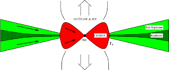
Figure 3: Cartoon diagram of two-component advective flow (TCAF) model. The Keplerian disk is flanked by the sub-Keplerian flow. In the CENBOL region, both the components mix, and its density as well as temperature increases. The outflow and the jet are produced from the CENBOL region.

In the region $r<r_{s}$, the Keplerian disk is assumed to be evaporated because of heating. The Keplerian matter mixes up with the sub-Keplerian halo inside the CENBOL and form a single component (CT95). The outflows and jets are believed to be produced from the CENBOL region (CT95; Chakrabarti 1999, hereafter C99).

A part of the low energy, blackbody photons (soft photons) that are emitted from the Keplerian disk, is intercepted by the hot electrons in the CENBOL. These photons are energized by the inverse-Compton scattering with these electrons and emerge as hard radiations. Thus, the radiated spectra are produced from both the components and are a function of accretion rates (CT95; Chakrabarti 1997). The relative importance of the accretion rates of these two components determine whether the spectrum is going to become hard or soft. The transition from the hard to soft state is found to be smoothly initiated by the mass accretion rates of the disk (CT95). The fast variability of the photon counts are explained by the time variation of the flow dynamics. If the shock moves back and forth then the hard radiations are expected to be modulated by the frequency of this oscillations since they are mainly produced in the post-shock region (CM00; Chakrabarti 2005). This way an important observed feature of several black hole candidates, namely, the quasi-periodic oscillation (QPO) is explained. According to the TCAF solution, different length scales of the flow are responsible for the different QPO frequencies (Chakrabarti 2005).

2 Radiative processes

When the accretion takes place, the gravitational energy of the matter is released partly in the form of radiation. This radiation covers the entire electromagnetic spectrum that ranges from radio to $\gamma$-rays, as discussed previously. The production of radiation in different frequency-bands, basically depends on the nature of the medium and the physical processes associated with the system. In black hole astrophysics, the radiation is mostly dominated in the X-ray frequency. Below we discuss some of the relevant radiative mechanisms. The emission mechanism of X-rays can be subdivided into two categories: thermal emission and non-thermal emission (Rybicki & Lightman 1979, hereafter RL79; Longair 2011).

1 Thermal emission

Thermal radiation is the radiation emitted by the matter in thermal equilibrium. The emitted radiation carries the information about the thermal nature of the body from where it is emitting. This emission mechanism can be subdivided in the following categories:

a) Blackbody radiation:

Blackbody radiation comes out from a system which is in thermodynamic equilibrium. Once the radiation enters into the system, it does not emit from it unless an equilibrium is established. In astrophysics, the blackbody radiation is emitted mainly by optically thick medium (e.g., standard thin disk). In such a medium, a single photon suffers from several scatterings. The intensity of the blackbody photons emitted from a system characterized by the temperature $T$ is given by the Planck’s Law,

$$B_{\nu}=\frac{2h\nu^{3}/c^{2}}{exp(h\nu/kT)-1}.$$

b) Bremsstrahlung radiation:

The acceleration or deceleration of a charged particle causes it to emit a photon. This is called bremsstrahlung or free-free emission. When a charged particle moves in the Coulomb field of another charged particle, the electric field causes the moving particle to emit bremsstrahlung. The radiation from a highly ionized medium which is in local thermal equilibrium (particles have Maxwell-Boltzmann velocity distribution) and optically thin (so that the radiation field is not in equilibrium), has a characteristic shape of continuous spectrum that is determined only by the temperature. This particular type of bremsstrahlung process is called the thermal bremsstrahlung.

The thermal bremsstrahlung spectrum falls off exponentially at higher energies and is characterized by the temperature $T$. The intensity $I$ of the radiation is given by,

$$I(\nu,T)=6.8\times 10^{-38}Z^{2}n_{e}n_{i}T^{-1/2}e^{-n\nu/kT}g(\nu,T)\rm{~{}erg~{}s^{-1}~{}cm^{-3}~{}Hz^{-1}},$$

where, $Z$ is the atomic number, $n_{e},n_{i}$ are the electron and ion number densities respectively and $g(\nu,T)$ is called the ‘Gaunt factor’. It is a slowly varying function of energy($h\nu$). A detail discussion is given in RL79.

c) Thermal Comptonization:

Comptonization (i.e., Compton scattering) occurs when a photon is scattered by an electron. A significant part of the energy is transferred from one to the another. When electron gains energy from the photon, it is called the Compton scattering, whereas, when the reverse process occurs, i.e., photon gains energy from the electrons, it is called the inverse-Compton scattering. In astrophysics, photons are energized by the second process, i.e., by inverse-Comptonization, and by the term Comptonization, we generally mean this process.

When the photon has a long wavelength (i.e., photon energy $h\nu<<m_{e}c^{2}=511\rm{keV}$), the scattering is closely elastic. It is called Thomson scattering. Electrons oscillate in the electric field of the wave, radiating the scattered wave as it does so. The scattering cross-section is $\sigma_{T}=8\pi r_{e}^{2}/3$, where, $r_{e}$ is the classical radius of the electron. But, when quantum effects enter, one considers Comptonization process.

Let us assume that a photon of energy $E=h\nu$ and momentum $\frac{E}{c}\boldsymbol{\Omega}$ is scattered by an electron of energy $\gamma m_{e}c^{2}$ and momentum ${\boldsymbol{p}}=\gamma m_{e}\boldsymbol{v}$, with $\gamma=\left(1-\frac{v^{2}}{c^{2}}\right)^{-1/2}$. After scattering the photon has energy $E^{\prime}=h\nu^{\prime}$ and momentum $\frac{E^{\prime}}{c}\boldsymbol{\Omega^{\prime}}$. Defining $\mu=\boldsymbol{\Omega.v}$, $\mu^{\prime}=\boldsymbol{\Omega^{\prime}.v}$ and scattering angle $\alpha=\cos^{-1}\boldsymbol{\Omega.\Omega^{\prime}}$, we find that,

$$\frac{\nu^{\prime}}{\nu}=\frac{1-\mu v/c}{1-\mu^{\prime}v/c+\frac{h\nu}{\gamma m_{e}c^{2}}(1-\cos\alpha)}.$$

If the electron is at rest ($v=0$), then,

$$\frac{\nu^{\prime}}{\nu}=\frac{1}{1+\frac{h\nu}{m_{e}c^{2}}(1-\cos\alpha)}.$$

The scattering cross-section is given by the Klein-Nishina formula (Poznyakov, Sobol & Sunyaev 1983, hereafter PSS83),

$$\sigma=\frac{2\pi r_{e}^{2}}{x}\left[\left(1-\frac{4}{x}-\frac{8}{x^{2}}\right)ln\left(1+x\right)+\frac{1}{2}+\frac{8}{x}-\frac{1}{2\left(1+x\right)^{2}}\right],$$

where, $x$ is given by,

$$x=\frac{2E}{m_{e}c^{2}}\gamma\left(1-\mu\frac{v}{c}\right).$$

Here, $r_{e}=e^{2}/m_{e}c^{2}$ is the classical electron radius and $m_{e}$ is the mass of the electron.

As mentioned earlier, in Comptonization, $\delta\nu<0$, i.e., a photon losses its energy. However, when we consider the scattering of a photon by a moving electron and the electron has a sufficient kinetic energy compared to the photon energy, an inverse-Comptonization occurs. Also, in astrophysics, we have to consider the scattering of isotropic distribution of photons with isotropic distribution of electrons. For non-relativistic electrons in thermal equilibrium at temperature $T$, the expression for the energy transfer per scattering is given by (RL79),

$$\frac{(\Delta h\nu)_{NR}}{h\nu}=\frac{(4kT-h\nu)}{m_{e}c^{2}}.$$

If the electrons have a temperature high enough so that $4kT>h\nu$, the photons gain energy, while at a low electron temperature it is the other way around. In any case, the fractional energy gain is very small, so that many scatterings are required for a significant effect, leading to diffusion of the energy in phase space. Hence, the emitted spectrum depends upon the factor $y=\tau_{es}(\Delta h\nu)_{NR}/h\nu,$ where, $\tau_{es}$ is the electron scattering optical depth.

2 Non-thermal emission

Non-thermal radiations are emitted when the emitter particles are not in thermal equilibrium, i.e., not Maxwellian. Photons do not interact with the electrons completely since the matter falls very rapidly. Non-thermal emission is very important in any environment where there are high energy particles.

a) Cyclotron radiation:

This is basically the bremsstrahlung process due to the presence of a magnetic field. If an electron gas permeated by a magnetic field, the electrons will be forced to gyrate about the field lines, and the radiation that is emitted as a result of this acceleration is known as the Cyclotron radiation, provided the electrons are moving at non-relativistic speeds. The radiation is emitted at the gyro-frequency, which is proportional to the magnetic field strength, $B$, and is given by, $\omega_{c}=eB/m_{e}$. The radiation emitted is linearly polarized when viewed perpendicular to the direction of the field lines, and circularly polarized when viewed end-on. In this particular type of emission process, unless the field strength ($B$) is large, the acceleration is not particularly large, nor is the intensity which depends on the square of the acceleration.

b) Synchrotron radiation:

When the velocity of the electrons gyrating in the magnetic field is relativistic ($v\sim c$), the radiation emitted is called synchrotron radiation. The frequency spectrum for this radiation is much more complex than the cyclotron radiation and can extend to many times the gyration frequency. The frequency of rotation, or gyro-frequency, in case of synchrotron radiation is given by $\omega_{s}=eB/\gamma m_{e}c$. As a result, the radiation produced is tightly beamed in a narrow angle about the forward direction of motion, by an amount determined by the Lorentz factor, $\gamma=1/\sqrt{(1-v^{2}/c^{2})}$. Hence in each rotation, a flash of light is observed with a duration $\delta t\approx(\gamma^{3}\omega_{s}\sin\alpha)^{-1}$. If the $\gamma$ is large, the width of the observed pulse ($\delta t$) can be much smaller than the gyration period $T_{s}={2\pi\over\omega_{s}}$ (RL79).

In this process, the power radiated by mono-energetic electrons is given by,

$$P=\frac{4}{3}\sigma_{T}c\beta^{2}\gamma^{2}U_{B},$$

where, $\sigma_{T}$ is the Thomson scattering cross section, $\beta(=v/c)$ is the velocity of the electron, and $U_{B}(=B^{2}/8\pi)$ is the magnetic energy density. The energy spectrum of synchrotron radiation results from the superposition of the individual electron spectra, and the energy spectrum can be approximated as power law distribution, i.e., $N(E)\propto E^{-p}$. Therefore, the resulting synchrotron emission spectrum will also be a power law type with a spectral index $s={1\over 2}(p-1).$

c) Non-thermal Comptonization:

We considered the scattering of photons with electrons in thermal equilibrium. However, electrons may be energized at the shock front by the shock acceleration process (Blandford & Eichler 1987; C96) very close to the black hole, where their kinetic energy become very high. These highly energetic electrons are called non-thermal electrons and with the presence of these, the process of Comptonization will be modified with respect to the thermal case.

The effect of non-thermal electrons on Comptonization will produce a high energy tail in the spectrum that is above the thermal cut-off. This high-energy tail is simply the characteristic of the superposition of the individual electron spectra of non-thermal electrons which have optical depth $(\tau)<<1$. Therefore, the spectral shape depends on the energy index $p$ of the power-law like, with an spectral index $s={1\over 2}(p-1)$.

3 Numerical simulations

The accretion disk models that have been mentioned above, give the steady state behavior of the accretion flow. Also, restrictions are imposed in the form of assumptions in order to tackle analytically the non-linear processes involved in the accretion and associated dissipative processes. This way we loose the ‘details’ that are present in the system and their dynamics. Numerical simulations help us to relax some restrictions by considering less number of assumptions. The use of a numerical code to solve the equations of fluid dynamics including the associated dissipative processes allow us to be much less restrictive in finding the detail features and their dynamics.

In the literature, results of numerical simulation of hydrodynamics and the radiative processes are present. In the following subsections, we give a brief overview of their developments and discuss the results that were obtained in these simulations.

1 Hydrodynamic simulation

The hydrodynamic simulation of the ‘thick’ accretion disk (including shock) was done much earlier than the models of thick accretion disk were made. Wilson (1972) developed a finite difference, fully general relativistic code which uses the method of first order backward space-differencing technique to study the behavior of inviscid rotating accreting matter onto a black hole. It was shown that the accretion flow having a significant angular momentum is accompanied by a generally moving shock. This code was later improved and a series of important simulations were performed (Hawley, Smarr & Wilson 1984a, 1984b; Hawley & Smarr 1986). In these simulations also, the shocks were found in the accretion of rotating matter. They found that the centrifugal barrier, or funnel wall, plays a key role in shock heating the inflowing supersonic fluid, producing a stationary thick disk with bipolar outflow. Subsequently, Eggum, Coroniti & Katz (1987) studied the evolution and stability of existing, sub-Eddington standard Keplerian disk including the effect of viscosity and radiation transport in their numerical simulations. In another paper, Eggum, Coroniti & Katz (1988) studied super-Eddington accretion disk using the same numerical code. They found that a thick disk really forms and found significant radiation driven winds and jet from the accretion disk.

A systematic study of the thick accretion disk including shock using numerical simulation was started after the extensive theoretical works on transonic accretion flows were done by Chakrabarti (1989b; C90). In the earlier works of Wilson, Hawley and others as mentioned above, the shocks were found in the accretion flow, but they were not stable and traveled outward. No standing shocks were found. The extensive works on transonic flows provided a very good theoretical basis of the subject and provided an understanding of the parameter space spanned by the specific energy ($\epsilon$) and the specific angular momentum ($\lambda$) of the sub-Keplerian inflow at the outer boundary. One good reason why previous simulations did not find any standing shock may be the wrong choice of the flow parameters or presence of a significant amount of numerical viscosity (C96). However, the theoretical works predicted that there are two types of solutions, with and without a shock, for a particular set of parameters $(\epsilon,\lambda)$.

Chakrabarti & Molteni (1993) showed by numerical simulation of inviscid, thin accretion flow that the shock could be common in the accretion flow onto a black hole. They found that the flow chooses the shock free solution in a truly unperturbed accretion (in one dimension). A shock is generated when some perturbation is introduced in the flow. In a realistic accretion flow which is three dimensional, the turbulence is always expected to be present and this acts as the seed of the required perturbation. Therefore, it is almost certain that realistic accretion disks have centrifugal pressure supported shocks in them (Chakrabarti & Molteni 1993; C96). Moreover, a shock solution has a higher entropy (Chakrabarti 1989b; C90) which makes it favorable choice as compared to the shock free solution for a given set of $(\epsilon,\lambda)$.

That the shock actually forms in a realistic accretion flow, was shown by two dimensional numerical simulations of accretion flows (Molteni, Lanzafame & Chakrabarti 1994, hereafter MLC94; Molteni, Ryu & Chakrabarti 1996, hereafter MRC96; Ryu, Chakrabarti & Molteni 1997, hereafter RCM97). They assumed axisymmetry and reduced the three dimensional problem to two dimensions. In these works, not only standing shocks but also oscillatory shocks were found to be formed. The consequent oscillations in the hydrodynamic and thermal properties of the accreting matter is believed to be the origin of the quasi-periodic variabilites observed in black hole candidates. Outflows and jets are seen to be produced from the post-shock region. More importantly, two different numerical simulation codes written on totally different principles produce similar results and those match with the theoretically obtained results (MRC96). One is a Lagrangian code based on smooth particle hydrodynamics (SPH) scheme (Lucy 1977; Gingold & Monaghan 1977; Monaghan 1983, 1992) and the other is an Eulerian finite difference code based on total variation diminishing (TVD) scheme (Harten 1983; Ryu, Ostriker, Kang & Cen 1993).

However, the occurrence and stability of the shocks depend on the transport phenomena e.g., viscous or radiative transport that are present in the flow. The simulations of thin, isothermal, viscous accretion disk using SPH code (Chakrabarti & Molteni 1995) show that the shock becomes weaker, wider and forms farther out in presence of weak viscosity. Shakura-Sunyaev (SS73) viscosity parameter $\alpha$ is used to tune the effect of viscosity. When the viscosity is increased, the shock starts traveling outward making the post-shock disk subsonic and the angular momentum distribution of this disk becomes similar to the Keplerian distribution. The flow becomes supersonic only close to the black hole, before falling onto it. The simulations of thick disk including viscous effects (Lanzafame, Molteni & Chakrabarti 1998) generalize the above results and show that even in thick disk, the centrifugally driven standing shock drifts away and eventually disappears. Similar conclusions are found more recently by Giri & Chakrabarti (2012) where the simulations of viscous, thick accretion disk were done using TVD code. Actually, it was found that above a certain value of $\alpha$, the critical viscosity $\alpha_{c}$, as predicted before by C90 and C96, the shock disappears. The critical viscosity parameter depends upon the injected flow parameters. Another important finding of the above simulations is the oscillation of the shock when the viscosity is low.

The oscillation of the shock was found in an inviscid flow also. In RMC97, the authors reported the presence of unstable shocks for the accretion of thin, cold, adiabatic gas in an axisymmetric, two dimensional simulation. The angular momentum of the incoming gas was around the marginally stable value. The reason of the formation of such an unstable shock is that the Rankine-Hugoniot conditions are not satisfied. In another significant simulation of inviscid accretion flows which include radiative transfer (Molteni, Sponholz & Chakrabarti 1996, hereafter MSC96) the shock oscillation was found when the cooling time scale of the post-shock region roughly matches with the infall time scale of the matter onto the black hole. The simulations were performed in both one and two dimensions. They used the power-law cooling $\Lambda\propto\rho^{2}T^{\zeta}$, where, $\rho$ and $T$ are the density and temperature, respectively, of the accreting matter. $\zeta=0.5$ represents the bremsstrahlung cooling. In Chakrabarti, Acharyya & Molteni (2004, hereafter CAM04), effect of Comptonization is included and the reflection symmetry about the equatorial plane is removed in an axisymmetric, two dimensional simulation of thick disk using SPH code. Compton cooling per unit mass from the post-shock matter with accretion rate $\dot{m}_{c}$ is mimicked by multiplying an efficiency factor $\eta$ to bremsstrahlung cooling with accretion rate $\dot{m}_{b}={\dot{m}_{c}\over\eta}$. Similar conclusions as MSC96 are obtained along with an extra effect of vertical shock oscillation apart from the radial oscillation.

The above mentioned shock oscillations in the thick accretion disk result in an significant observational effect, namely, the QPOs. As mentioned earlier, in TCAF model the high energy photons of the observed spectra from the black hole candidates are produced in the post-shock region. Therefore the hydrodynamic and thermal variability present in this region will be reflected in the observed variations of the high energy photon count rate. This is actually observed in the realistic data (CM00; Rao, Naik, Vadawale & Chakrabarti 2000).

2 Radiative transfer

One of the most important radiative processes in the context of galactic black holes is the Compton scattering between the electrons and the radiation field. In order to explain the power-law part in the hard state spectrum from the black hole candidates, multiple inverse-Compton scattering of the low energy photons by the weakly relativistic or relativistic, hot electrons is assumed to be mainly responsible. Several theoretical models have been developed to compute the spectral shape from the corona (Katz 1976; Sunyaev & Trumper 1979; Sunyaev & Titarchuk 1980,1985). In these references, calculations have been done using the Kompaneets equation (Kompaneets 1956; RL79). However, theoretical calculations are restricted by several constraints. For example, the spectra can be described adequately by analytic methods given in the above references for non-relativistic ($kT_{e}<<m_{e}c^{2}$) or ultra-relativistic ($kT_{e}>>m_{e}c^{2}$) cases, but in mildly relativistic plasma ($kT_{e}\sim m_{e}c^{2}$), it is hard to treat the problem analytically (PSS83). This restriction was removed later by Titarchuk and his collaborator (Titarchuk 1994; Hua & Titarchuk 1995; Titarchuk & Lyubarskij 1995) where they derived the spectral indices for wide ranges of the optical depth and electron temperatures of the cloud. However, the computations are done for a particular geometry such as a slab or spherical type and the variation of the optical depth or the temperature inside a cloud is not taken into account, rather some average values are considered. However, it is seen from numerical simulations that the geometry of the electron cloud in the accretion disk is much more complicated and different regions have different temperatures as well as different optical depths. Therefore by taking simplified assumptions such as a particular geometry or averaged temperature or optical depth while computing the spectral shape, we actually lose the details of an accretion flow configuration. In such conditions, the correct spectra would be obtained by Monte Carlo methods.

A Monte Carlo method is a numerical method of solving mathematical problems by random sampling (Sobol 1994). This method can be applied to solve any mathematical problem, not just those of probabilistic character (PSS83). The Monte Carlo simulation technique has been applied to study the Compton scattering problem. Poznyakov, Sobol & Sunyaev (1976, 1977, 1983) computed the X- and $\gamma$ ray radiations for spherical cloud and slab disks of thermal relativistic plasma of a given optical depth with a given temperature. The low frequency photon source was either a point source (for a spherical cloud) at the center or a flat disk (slab geometry) or distributed within an electron cloud. These simulations show that the power-law part of the spectrum is produced by the inverse-Comptonization of the low frequency photons, firmly establishing early theoretical work on Comptonization (Katz 1976; Sunyaev & Trumper 1972; Sunyaev & Titarchuk 1980). In the simulation, the energy of the injected Planck photons, the momentum of the Maxwell electrons inside the electron cloud, mean free path of the photon and the Compton scattering – all these events have been modelled by Monte Carlo techniques (PSS83). However, in these calculations, the Comptonization by the thermal Maxwellian electrons alone has been considered. In subsequent works, Laurent & Titarchuk (1999, 2001, 2007) incorporated the effects of bulk velocity of electrons in addition to its thermal motions in the Monte Carlo code and computed the effects of up-scattering of converging inflow on the output spectrum. They assumed the geometry of the Compton cloud to be spherical and the electrons to approach the central black hole with free fall velocity. The simulation of the Compton scattering is similar to the method described in PSS83 with the difference that it takes into account the exact motion of the electron, which is the composition of its free fall motion with its Brownian thermal motion. Simulations in both flat as well as curved space were done. They showed that in both the soft and the hard states, the spectra are formed by the up-scattering of the disk soft photons by the converging electrons. The effect of momentum transfer is found to be so strong that even a cooler Compton cloud can produce a power-law component extending to energies comparable with the kinetic energy of electrons in the converging flow.

The first computation of spectral properties of the TCAF using Monte Carlo method was done by Ghosh, Chakrabarti & Laurent (2009). In this study, they computed the effects of thermal Comptonization of soft photons coming from an extended Keplerian disk by hot electrons of the CENBOL. The effect of bulk motions was not taken into account, however. The simulations show that the state transition of the black hole candidate can be explained either by varying the size of the CENBOL or by changing the central density of the CENBOL, which is governed by the sub-Keplerian accretion rate.

Chapter 1 COMPUTATIONAL PROCEDURE OF SPECTRAL PROPERTIES OF THE TCAF MODEL

In this Chapter, we shall discuss the algorithm of the serial Monte Carlo code and its parallelization process. Next, we shall discuss how this code is used to study the spectral properties of TCAF in presence of outflows.

2.1 Monte Carlo code for Comptonization and its parallelization

Here we briefly discuss the algorithm of computation of Comptonized spectrum using a Monte Carlo code. The algorithm is similar to the one used by Laurent & Titarchuk (1999) and Ghosh et al. (2009). Then, the implementation of parallelization will be described in detail.

In our simulation, each photon is tracked beginning from its origin till its detection. The photon source may be a point source or any disk (e.g., a standard SS73 disk) or distributed within the electron cloud (e.g., bremsstrahlung, synchrotron etc.). Its initial energy may be drawn from the Planck’s distribution function (for blackbody type source) or from any other given distribution e.g., power-law etc. It can be given any initial preferential direction or it may be emitted isotropically. So, once a photon is generated within the accretion disk, we know its location (co-ordinate), initial energy and initial direction of motion. Certain scattering condition is associated with each photon. For the present case, we set a target optical depth $\tau_{c}$ at which a particular photon will suffer scattering. This value is computed from the exponential law $P(\tau)=exp(-\tau)$ (Laurent & Titarchuk 1999). Next, the optical thickness $\tau=n_{e}\sigma l$ along the photon path is integrated taking into account the variation in the electron number density $n_{e}$ and the scattering cross-section $\sigma$. If integrated $\tau$ for that particular photon becomes $\tau_{c}$ before leaving the electron cloud, a Compton scattering is simulated following PSS83. After the scattering, the direction as well as energy of the photon change and it is again tracked in the same way as mentioned above. On the other hand, if $\tau<\tau_{c}$ before leaving the Compton cloud, the photon remains unscattered. This way, each photon is tracked till its escape from the electron cloud or it is absorbed by the black hole. Once a photon is out, it is captured and used for spectrum determination.

In the Monte Carlo code, the initial properties of a photon (e.g., its location, energy etc.), scattering criteria (e.g., target optical depth, mean free path of photons etc.) and the scattering event (e.g., selection of scattering electron, its momentum and energy etc.) are modelled using Monte Carlo technique (PSS83). The pseudo-random number generator that has been used here is taken from Wichmann & Hill (1982).

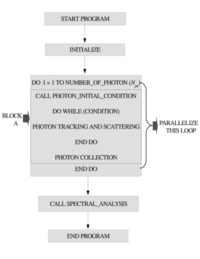
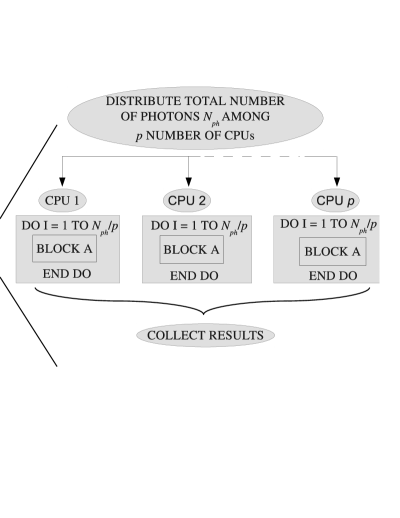
Figure 2.1: Flowchart of the serial code (left) and its parallelization (right).

In a serial run, a single processor processes photons one by one and at the end, we get the full spectrum. For a steady state system, the behavior of one photon inside the accretion disk is independent of another one, i.e., processing of photons are mutually exclusive. So, it does not matter if we process more than one photon simultaneously. In a prallelized code, that is what is done. Depending on the number of available processors, the number of simultaneously injected photons is decided. So, if we wish to inject $N_{ph}$ number of photons and we have $p$ number of available processors, then each processor processes $N_{ph}/p$ number of photons simultaneously in the same electron cloud. In Fig. 2.1, we show the flowcharts of the serial code and after its parallelization. In the serial code, ‘Block A’ is the main computational block which is called $N_{ph}$ times under a ‘Do’ loop. In the parallel code, we have broken this single ‘Do’ loop in $N_{ph}/p$ loops and run the same block A in $p$ number of processors. At the end, we collect the results from each processors and sum them to get the final spectrum.

One important practical problem of parallelization in this case is the choice of set of seed values for the pseudo-random number generator used here. In a serial run, the initial seed values are chosen such that the cycle length is very long, and the cycle length depends on the initial seed values. In parallelized case, since the same program with the same input files runs on different processors, same seed values will produce exactly same results. For this, we have to be careful about the initial seed values for individual processors. We cannot choose any arbitrary seed values for each processors since that may hamper the cycle length. To circumvent this problem, we pick up some numbers from the series that is generated when the pseudo-random number generator is run. We use these numbers as the initial seed values for different processors. We have to make sure that these selected numbers are far away from each other in the series so that no repetition occurs and we do not get same results from different processors.

1 Parallelization technique

The parallelization has been done using Message-Passing Interface (MPI). As the name suggests, the communication between the multiple processors is done by message-passing. MPI is a library of functions and macros that can be used in C, FORTRAN, and C++ programs. Here, we have used MPI FORTRAN functions for parallelizing our Monte Carlo code written in FORTRAN.

There are many functions in MPI, out of which only a handful have been utilized here. Here, in brief, we describe the functions that we have used. More details can be found in Pacheco & Ming (1997).

MPI_init and MPI_finalize – The first function must be called before any other MPI function is called. After a program has finished using MPI library, the second function must be called. The syntaxes are as follows:

MPI_init(Ierr)
MPI_finalize(Ierr)

The argument contains an error code. This argument is generally used in every FORTRAN MPI routines.

MPI_COMM_Rank – This function gives rank to the processors being used. Its syntax is as follows:

MPI_COMM_Rank(Comm, Myrank, Ierr)

The first argument is a communicator. A communicator is a collection of processors that communicate among themselves and take part in message passing when the program begins execution. In our program, we have used the communicator ‘MPI_COMM_WORLD’. It is pre-defined in MPI and consists of all the processors running when program execution begins.

MPI_COMM_SIZE – This function is used to know the number of processors that is executing the program. Its syntax is:

MPI_COMM_SIZE(Comm, P, Ierr)

‘P’ gives the number of processors. This number may be used for various purposes. In our program, we have explicitly used this number while message-passing.

MPI_Send and MPI_Recv – These are the two functions we find mostly used in message-passing between different processors. The syntaxes are as follows:

MPI_Send(Message, Count, Datatype, Dest, Tag, Comm, Ierr)
MPI_Recv(Message, Count, Datatype, Source, Tag, Comm, Status, Ierr)

The first one sends a message to a designated processor, whereas the second one receives from a processor. The contents of ‘Message’ is stored in a block of memory referenced by the argument message. ‘Message’ may be a single number, an array of numbers or characters. ‘Count’ and ‘Datatype’ are the count values and the MPI type datatype of ‘Message’, respectively. This type is not the Fortran type. In the following list, some of the MPI types and their corresponding Fortran types are listed.

MPI datatype	Fortran datatype
MPI_integer	Integer
MPI_real	Real
MPI_double_precision	Double precision
MPI_complex	Complex

‘Dest’ and ‘Source’ are two integer variables to mark the rank of the destination and the source processors of ‘Message’, respectively. The ‘Tag’ is also an integer that is used to distinguish messages received from a single processor.

MPI_Barrier – This function provides a mechanism for synchronizing all the processors in the communicator. Each processor pauses until every processors in communicator have called this function. It has the following syntax:

MPI_Barrier(Comm, Ierr)

MPI_Bcast – This is a collective communication function, meaning the communication where usually all the processors are involved. Using this command a single processor can send the same data to every processors in a single call. The ‘Send-Recv’ commands usually involve two processors - one sender and other receiver, whereas in collective communications like broadcast, number of sender is one but receivers are all the other processors in the communicator. The syntax is as follows:

MPI_Bcast(Message, Count, Datatype, Root, Comm, Ierr)

All the processors in a communicator have to call this function with the same argument ‘Root’. The contents of ‘Message’ in processor ‘Root’ is broadcasted to all the processors.

MPI_Reduce – This is another collective communication function. This is a global reduction operation in which all the processors contribute data which is combined using a binary operation. The typical binary operations are addition, max, min, product etc. The syntax is as follows:

MPI_Reduce(Operand, Result, Count, Datatype, Operation, Root, Comm, Ierr)

MPI_Reduce combines ‘Operand’ stored in different processors to ‘Results’ in ‘Root’ using operation ‘Operation’. In the following table, we present some predefined operations.

Operation Name	Meaning
MPI_sum	Addition
MPI_max	Maximum
MPI_min	Minimum
MPI_prod	Product

MPI_Gather – This collective communication function is used to gather data in one processor from all other processors. The syntax is as follows:

MPI_Gather(Send_Val, Send_Count, Send_Type, Recv_Val, Recv_Count, Recv_Type, Root, Comm, Ierr)

Each processor sends the contents of ‘Send_Val’ to processor ‘Root’ and the ‘Root’ concatenates the received data in processor rank order, i.e., data from processor 0 is followed by data from processor 1, which is followed by processor 2 and so on.

2.2 Spectral properties of TCAF in presence of a jet

We use the above mentioned Monte Carlo code to study the spectral properties of a TCAF in presence of a jet around a galactic black hole (Ghosh, Garain, Chakrabarti & Laurent 2010, hereafter GGCL10) . Computation of the spectral characteristics have so far concentrated only on the advective accretion flows (CT95; Chakrabarti & Mandal 2006; Dutta & Chakrabarti 2010) and the jet was not included. In the Monte Carlo simulations of Laurent & Titarchuk (2007) outflows in isolation were considered and not in conjunction with inflows. In the following work, we obtain the outgoing spectrum in presence of both inflows and outflows (GGCL10). We also include a Keplerian disk inside an advective flow which is the source of the soft photons. We show how the spectrum depends on the flow parameters of the inflow, such as the accretion rates and the shock strength. These results, as such, were anticipated earlier (C99; Das, Chattopadhyay, Nandi & Chakrabarti 2001). The post-shock region being denser and hotter, behaves as the so-called ‘Compton cloud’ in the classical model of Sunyaev and Titarchuk (1980) and is known as the CENtrifugal pressure supported BOundary Layer or CENBOL. The variation of the size of the Compton cloud, and therefore the basic Comptonized component of the spectrum is thus a function of the basic parameters of the flow, such as the energy, accretion rate and the angular momentum. Since the intensity of soft photons determines the Compton cloud temperature, the result depends on the accretion rate of the Keplerian component also. In our result, we see the effects of the bulk motion Comptonization (CT95) because of which even a cooler CENBOL produces a harder spectrum. At the same time, the effects of down-scattering due the outflowing electrons are also seen, because of which even a hotter CENBOL causes the disk-jet system to emit lesser energetic photons.

1 Simulation set up

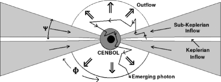
Figure 2.2: A schematic diagram of the geometry of our Monte Carlo Simulations presented in this Chapter. The spherical inflowing post-shock region surrounds the black hole and it is surrounded by the Keplerian disk on the equatorial plane. A diverging conical outflow is present on the top of the post-shock region. A tenuous sub-Keplerian flow above and below the Keplerian disk is also present (CT95). Typical photon scatterings are shown by zig-zag paths (GGCL10).

In Fig. 2.2, we present a schematic diagram of our simulation set up (GGCL10). The components of the hot electron clouds, namely, the CENBOL, the jet and the sub-Keplerian flow, intercept the soft photons emerging out of the Keplerian disk and reprocess them via inverse-Compton scattering. A photon may undergo a single, multiple or no scattering at all with the hot electrons in between its emergence from the Keplerian disk and its detection by the telescope at a large distance. The photons which enter the black holes are absorbed. The CENBOL, though toroidal in nature (CT95), is chosen to be of spherical shape for simplicity. The sub-Keplerian inflow in the pre-shock region is assumed to be of wedge shape of a constant angle. The outflow, which emerges from the CENBOL in this picture is also assumed to be of constant conical angle.

2 Temperature, velocity and density profiles inside the Compton cloud

We assume the black hole to be non-rotating and we use the pseudo-Newtonian potential (PW80) to describe the geometry around a black hole (Chapter 1). This potential is $-\frac{1}{2(r-1)}$ ($r$ is in the unit of Schwarzschild radius $r_{g}=2GM_{bh}/c^{2}$). Velocities and angular momenta are measured accordingly.

As a simple example, we use the Bondi accretion and wind solutions to compute the density, velocity and temperature in the inflowing (inside sub-Keplerian inflow and CENBOL) and outflowing regions of the CENBOL, respectively (GGCL10). Bondi solution (Bondi 1952) was originally done to describe the accretion of matter which is at rest at infinity onto a star at rest. The motion of matter is steady and spherically symmetric. The equation of the motion of this matter around the black hole in the steady state is given by (C90),

$$u\frac{du}{dr}+\frac{1}{\rho}\frac{dP}{dr}+\frac{1}{2(r-1)^{2}}=0.$$

Here, $u$ is the velocity, $\rho$ is the density and $P$ is the thermal pressure. This is the Eulerian equation written in the spherical polar coordinate system $[r,\theta,\phi]$. $\theta$ and $\phi$ derivatives have been removed because of spherical symmetry and the time derivative has been removed since we consider the steady state. Integrating this equation, we get the expression of the conserved specific energy as (C90),

$$\epsilon=\frac{u^{2}}{2}+na^{2}-\frac{1}{2(r-1)}.$$ (2-1)

Here, $a$ is the adiabatic sound speed, given by $a=\sqrt{\gamma P/\rho}$, $\gamma$ being the adiabatic index and is equal to $\frac{4}{3}$ in our case. The conserved mass flux equation, as obtained from the continuity equation, is given by (C90),

$$\dot{M}=\Omega\rho ur^{2},$$ (2-2)

where, $\Omega$ is the solid angle subtended by the flow. For an inflowing matter, $\Omega$ is given by,

$$\Omega_{in}=4\pi\sin\Psi,$$

where, $\Psi$ is the half-angle of the conical inflow (see, Fig. 2.2). For the outgoing matter, the solid angle is given by,

$$\Omega_{out}=4\pi(1-\cos\Phi),$$

where, $\Phi$ is the half-angle of the conical outflow (see, Fig. 2.2). From Eq. (2-2), we get

$$\dot{\mu}=a^{2n}ur^{2}.$$ (2-3)

The quantity $\dot{\mu}=\frac{\dot{M}\gamma^{n}K^{n}}{\Omega}$ is called the entropy accretion rate (Chakrabarti 1989b; C90), $K$ being the constant measuring the entropy of the flow, and $n=\frac{1}{\gamma-1}$ is called the polytropic index. We take derivative of Eq. (2-1) and (2-3) with respect to $r$ and eliminating $\frac{da}{dr}$ from both the equations (C90), we get the gradient of the velocity as,

$$\frac{du}{dr}=\frac{\frac{1}{2(r-1)^{2}}-\frac{2a^{2}}{r}}{\frac{a^{2}}{u}-u}.$$ (2-4)

This equation is solved numerically using 4^th order Runge Kutta method. Solving these equations, we obtain the radial variations of $u$, $a$ and finally the temperature profile using $T(r)=\frac{\mu a^{2}(r)m_{p}}{\gamma k_{B}}$, where $\mu=0.5$ is the mean molecular weight, $m_{p}$ is the proton mass and $k_{B}$ is the Boltzmann constant. Using Eq. (2-2), we calculate the mass density $\rho$, and hence, the number density variation of electrons inside the Compton cloud. We ignore the electron-positron pair production inside the cloud.

The flow is supersonic in the pre-shock region and sub-sonic in the post-shock (CENBOL) region. The shock forms at the location of the CENBOL surface (CT95). We chose this surface at a location where the Mach number $M=2$. This location depends on the specific energy $\epsilon$. In our simulation, we have chosen $\epsilon=0.015$ so that we get $R_{s}=10$ (GGCL10). We simulated a total of six cases: for Cases 1(a-c), we chose the halo accretion rate $\dot{m}_{h}=1$ and the disk accretion rate $\dot{m}_{d}=0.01$, and for Cases 2(a-c), the values are listed in Table 2 (GGCL10). The velocity variation of the sub-Keplerian flow is the inflowing Bondi solution (pre-shock point). The density and the temperature of this flow have been calculated according to the above mentioned formulas. Inside the CENBOL, both the Keplerian and the sub-Keplerian components are merged. The velocity variation of the matter inside the CENBOL is assumed to be the same as the Bondi accretion flow solution reduced by the compression ratio $R$ due to the shock. The compression ratio (i.e., the ratio between the post-shock and pre-shock densities) $R$ is also used to compute the density and the temperature profile.

When the outflow is adiabatic, the ratio of the outflow to the inflow rate is given by (Das et al., 2001),

$$R_{\dot{m}}=\frac{\Omega_{out}}{\Omega_{in}}\left(\frac{f_{0}}{4\gamma}\right)^{3}\frac{R}{2}\left[\frac{4}{3}\left(\frac{8(R-1)}{R^{2}}-1\right)\right]^{3/2},$$ (2-5)

where, $f_{0}={R^{2}\over R-1}$ and we have used $n=3$ for a relativistic flow. Using this and the velocity variation obtained from the wind branch of the Bondi solution, we compute the density variation inside the jet. In our simulation, we have used $\Phi=58^{\circ}$ and $\Psi=32^{\circ}$ (GGCL10). Figure 2.3 shows the variation of the percentage of matter in the outflow for these particular parameters.

Figure 2.3: Ratio of the outflow and the inflow rates as a function of the compression ratio of the inflow when the outflow is adiabatic. The jet angle $\Phi\sim 60^{\circ}$ was used (GGCL10).

3 Keplerian disk

The soft photons are produced from a Keplerian disk whose inner edge coincides with the CENBOL surface, while the outer edge is located at $500r_{g}$. The source of soft photons has a multi-color blackbody spectrum coming from a standard disk (SS73). We assume the disk to be optically thick and the opacity due to free-free absorption is more important than the opacity due to scattering. The emission is blackbody type with the local surface temperature (Eq. 1):

$$T(r)=5\times 10^{7}(M_{bh})^{-1/2}(\dot{m_{d}}_{17})^{1/4}(2r)^{-3/4}\left[1-\sqrt{\frac{3}{r}}\right]^{1/4}\mathrm{~{}K.}$$

Photons are emitted from both the top and bottom surfaces of the disk at each radius. Total number of photons emitted from the disk surface at a radius $r$ is obtained by integrating over all frequencies ($\nu$) and is given by,

$$n_{\gamma}(r)=\frac{4\pi}{c^{2}}\left(\frac{kT}{h}\right)^{3}\times 1.202\mathrm{~{}cm^{-2}~{}s^{-1}.}$$ (2-6)

Thus, the disk between radius $r$ to $r+\delta r$ produces $dN(r)$ number of soft photons:

$$dN(r)=4\pi r\delta rn_{\gamma}(r)\mathrm{~{}s^{-1}}.$$ (2-7)

The soft photons are generated isotropically between the inner and the outer edges of the Keplerian disk. Their positions are randomized using the above distribution function (Eq. 2-7). All the results of the simulations presented here have used the number of injected photons as $6.4\times 10^{8}$. We chose $M_{bh}=10M_{\odot}$ and $\delta r=0.5r_{g}$ (GGCL10).

4 Simulation procedure

The simulation procedure is the same as used in Ghosh at al. (2009) and GGCL10. To begin a Monte Carlo simulation, we generate photons from the Keplerian disk with randomized locations as mentioned in the earlier Section. The energy of the soft photons at radiation temperature $T(r)$ is calculated using the Planck’s distribution formula, where the number density of the photons [$n_{\gamma}(E)$] having an energy $E$ is expressed by (PSS83),

$$n_{\gamma}(E)=\frac{1}{2\zeta(3)}b^{3}E^{2}(e^{bE}-1)^{-1},$$

where, $b=1/k_{B}T(r)$ and $\zeta(3)=\sum^{\infty}_{1}{l}^{-3}=1.202$, the Riemann zeta function. Using another set of random numbers, we obtain the direction of the injected photon and with yet another random number, we obtain a target optical depth $\tau_{c}$ at which the scattering takes place. The photon is followed within the sub-Keplerian matter till the total optical depth ($\tau$) reached $\tau_{c}$. The increase in optical depth ($d\tau$) during its traveling of a path of length $dl$ inside the sub-Keplerian matter is given by: $d\tau=\rho_{n}\sigma dl$, where $\rho_{n}$ is the electron number density.

The total scattering cross section $\sigma$ is given by Klein-Nishina formula:

$$\sigma=\frac{2\pi r_{e}^{2}}{x}\left[\left(1-\frac{4}{x}-\frac{8}{x^{2}}\right)ln\left(1+x\right)+\frac{1}{2}+\frac{8}{x}-\frac{1}{2\left(1+x\right)^{2}}\right],$$

where, $x$ is given by,

$$x=\frac{2E}{m_{e}c^{2}}\gamma\left(1-\mu\frac{v}{c}\right).$$

Here, $r_{e}=e^{2}/m_{e}c^{2}$ is the classical electron radius and $m_{e}$ is the mass of the electron.

We have assumed here that a photon of energy $E$ and momentum $\frac{E}{c}\boldsymbol{\Omega}$ is scattered by an electron of energy $\gamma m_{e}c^{2}$ and momentum ${\boldsymbol{p}}=\gamma m_{e}\boldsymbol{v}$, with $\gamma=\left(1-\frac{v^{2}}{c^{2}}\right)^{-1/2}$ and $\mu=\boldsymbol{\Omega.v}$. At the point where a scattering is allowed to take place, the photon selects an electron and the energy exchange is computed using the Compton or inverse-Compton scattering formula. The electrons are assumed to obey relativistic Maxwell distribution inside the sub-Keplerian matter. The number $dN(\boldsymbol{p})$ of Maxwellian electrons having momentum between $\boldsymbol{p}$ to $\boldsymbol{p}+d\boldsymbol{p}$ is expressed by,

$$dN(\boldsymbol{p})\propto exp[-(p^{2}c^{2}+m_{e}^{2}c^{4})^{1/2}/kT_{e}]d\boldsymbol{p}.$$

5 Results and discussions

In a given simulation, we assume one Keplerian disk rate ($\dot{m}_{d}$) and one sub-Keplerian halo rate ($\dot{m}_{h}$) (GGCL10). The specific energy of the halo provides hydrodynamic (such as number density of the electrons and the velocity variation) and the thermal properties of matter. The shock location of the CENBOL is chosen where the Mach number $M=2$ for simplicity and the compression ratio $R$ (i.e., jump in density) at the shock is assumed to be a free parameter.

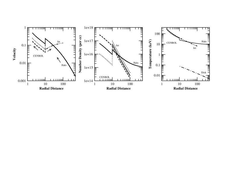
Figure 2.4: (a-c): Velocity (left), density (middle) and the temperature (right) profiles of the Cases 1(a-c) as described in Table 1 are shown with solid ($R=2$), dotted ($R=4$) and dashed ($R=6$) curves. $\dot{m_{d}}=0.01$ and $\dot{m_{h}}=1$ were used (GGCL10).

In Fig. 2.4(a-c), we present the velocity, electron number density and temperature variations as a function of the radial distance from the black hole for specific energy $\epsilon=0.015$. $\dot{m_{d}}=0.01$ and $\dot{m_{h}}=1$ were chosen. Three cases were run by varying the compression ratio $R$. These are given in Column 2 of Table 1. The corresponding percentage of matter going in the outflow is also given in Column 2. In the left panel, the bulk velocity variation is shown. Since we chose the pseudo-Newtonian potential, the radial velocity is not exactly unity at $r=1$, the horizon, but it becomes unity just outside. In order not to over estimate the effects of bulk motion Comptonization which is due to the momentum transfer of the moving electrons to the photons, we shift the horizon just outside $r=1$ where the velocity is unity. The solid, dotted and dashed curves are the velocity for $R=2$ (Case 1a), $4$ (Case 1b) and $6$ (Case 1c) respectively. The same line style is used in other panels. The velocity variation within the jet does not change with $R$, but the density (in the unit of $cm^{-3}$) does (middle panel). The double dot-dashed line gives the velocity variation of the matter within the jet for all the above cases. The arrows show the direction of the bulk velocity (radial direction in accretion, vertical direction in jets). The last panel gives the temperature (in keV) of the electron cloud in the CENBOL, jet, sub-Keplerian and Keplerian disk. Big dash-dotted line gives the temperature profile inside the Keplerian disk.

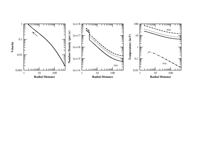
Figure 2.5: (a-c): Velocity (left), density (middle) and the temperature (right) profiles of Cases 2(a-c) as described in Table 2 are shown with solid ($\dot{m_{h}}=0.5$), dotted ($1$) and dashed ($1.5$) curves. $\dot{m_{d}}=1.5$ was used throughout. Velocities are the same for all the disk accretion rates (GGCL10).

In Fig. 2.5(a-c), we show the velocity (left), number density of electrons (middle) and temperature (right) profiles of Cases 2(a-c) as described in Table 2. Here we have fixed $\dot{m_{d}}=1.5$ and $\dot{m_{h}}$ is varied: ${\dot{m_{h}}}=\ 0.5$ (solid), $1$ (dotted) and $1.5$ (dashed). No jet is present in this case ($R=1$). To study the effects of bulk motion Comptonization, the temperature of the electron cloud has been kept low for these cases. The temperature profile of the Keplerian disk for the above cases has been marked as ‘Disk’ .

Table 1 (GGCL10)
Case	R, $P_{m}$	$N_{int}$	$N_{cs}$	$N_{cenbol}$	$N_{jet}$	$N_{subkep}$	$N_{cap}$	$p$	$\alpha$
1a	2, 58	2.7e+8	4.03e+8	1.35e+7	7.48e+7	8.39e+8	3.34e+5	63	0.43
1b	4, 97	2.7e+8	4.14e+8	2.38e+6	1.28e+8	8.58e+8	3.27e+5	65	1.05
1c	6, 37	2.7e+8	3.98e+8	5.35e+7	4.75e+7	8.26e+8	3.07e+5	62	-0.4

In Table 1, we summarize the results of all the cases in Fig. 2.4(a-c). In Column 1, various cases are marked. In Column 2, the compression ratio (R) and percentage $P_{m}$ of the total matter that is going out as outflow (see, Fig. 2.4) are listed. In Column 3, we show the total number of photons (out of the total injection of $6.4\times 10^{8}$) intercepted by the CENBOL and jet ($N_{int}$) combined. Column 4 gives the number of photons ($N_{cs}$) that have suffered Compton scattering inside the flow. Columns 5, 6 and 7 show the number of scatterings which took place in the CENBOL ($N_{cenbol}$), in the jet ($N_{jet}$) and in the pre-shock sub-Keplerian halo ($N_{subkep}$) respectively. A comparison of them will give the relative importance of these three sub-components of the sub-Keplerian disk. The number of photons captured ($N_{cap}$) by the black hole is given in Column 8. In Column 9, we give the percentage $p$ of the total injected photons that have suffered scattering through CENBOL and the jet. In Column 10, we present the energy spectral index $\alpha$ [$I(E)\sim E^{-\alpha}$] obtained from our simulations.

Table 2 (GGCL10)
Case	$\dot{m_{h}}$, $\dot{m_{d}}$	$N_{int}$	$N_{cs}$	$N_{ms}$	$N_{subkep}$	$N_{cap}$	$p$	$\alpha_{1},\alpha_{2}$
2a	0.5, 1.5	1.08e+6	2.13e+8	7.41e+5	3.13e+8	1.66e+5	33.34	-0.09, 0.4
2b	1.0, 1.5	1.22e+6	3.37e+8	1.01e+6	6.82e+8	2.03e+5	52.72	-0.13, 0.75
2c	1.5, 1.5	1.34e+6	4.15e+8	1.26e+6	1.11e+9	2.29e+5	64.87	-0.13, 1.3

In Table 2, we summarize the results of simulations where we have varied $\dot{m}_{h}$, for a fixed value of $\dot{m}_{d}$. In all of these cases no jet comes out of the CENBOL (i.e., $R=1$). In the last column, we list two spectral slopes $\alpha_{1}$ (from $10$ to $100$keV) and $\alpha_{2}$ (due to the bulk motion Comptonization). Here, $N_{ms}$ represents the photons that have suffered scattering between $R_{g}=3$ and the horizon of the black hole.

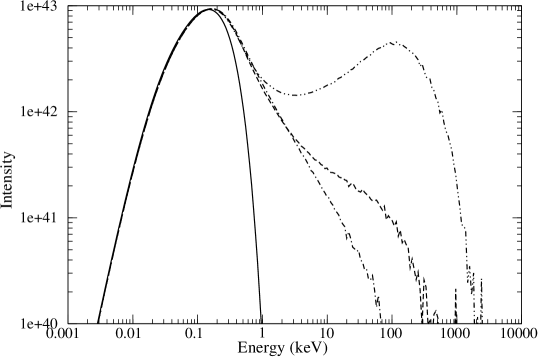
Figure 2.6: Variation of the emerging spectrum for different compression ratios. The solid curve is the injected spectrum from the Keplerian disk. The dashed, dash-dotted and double dot-dashed lines are for $R=2$ (Case 1a), $R=4$ (Case 1b) and $R=6$ (Case 1c), respectively. The disk and halo accretion rates used for these cases are $\dot{m}_{d}=0.01$ and $\dot{m}_{h}=1$ (GGCL10). See, text for details.

In Fig. 2.6, we show the variation of the spectrum in the three simulations presented in Fig. 2.4(a-c). The dashed, dash-dotted and double dot-dashed lines are for $R=2$ (Case 1a), $R=4$ (Case 1b) and $R=6$ (Case 1c), respectively. The solid curve gives the spectrum of the injected photons. Since the density, velocity and temperature profiles of the pre-shock, sub-Keplerian region and the Keplerian flow are the same in all these cases, we find that the difference in the spectrum is mainly due to the CENBOL and the jet. In the case of the strongest shock (compression ratio $R=6$), only $37\%$ of the total injected matter goes out as the jet. At the same time, due to the shock, the density of the post-shock region increases by a factor of $6$. Out of the three cases, the effective density of the matter inside CENBOL is the highest and that inside the jet is the lowest in this case. Due to the shock, the temperature increases inside the CENBOL and hence the spectrum is the hardest. Similar effects are seen for moderate shock ($R=4$) and to a lesser extent, the low strength shock also ($R=2$). When $R=4$, the density of the post-shock region increases by the factor of $4$ while almost $97\%$ of total injected matter (Fig. 2.4) goes out as the jet reducing the matter density of the CENBOL significantly. From Table 1, we find that the $N_{cenbol}$ is the lowest and $N_{jet}$ is the highest in this case (Case 1b). This decreases the up-scattering and increases the down-scattering of the photons. This explains why the spectrum is the softest in this case (Chakrabarti 1998b). In the case of low strength shock ($R=2$), $57\%$ of the inflowing matter goes out as jet, but due to the shock the density increases by factor of $2$ in the post-shock region. This makes the density similar to a case as though the shock did not happen except that the temperature of CENBOL is higher due to the shock. So the spectrum with the shock would be harder than when the shock is not present. The disk and the halo accretion rates used for these cases are $\dot{m_{d}}=0.01$ and $\dot{m_{h}}=1$.

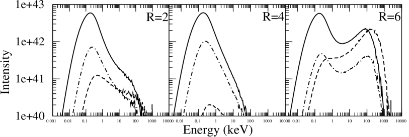
Figure 2.7: (a-c): Variation of the components of the emerging spectrum with the shock strength (R). The dashed curves correspond to the photons emerging from the CENBOL region and the dash-dotted curves are for the photons coming out of the jet region. The solid curve is the spectrum for all the photons that have suffered scatterings (GGCL10). See, the text for details.

In Fig. 2.7, we show the components of the emerging spectrum for all the three cases presented in Fig. 2.6. The solid curve is the intensity of all the photons which suffered at least one scattering. The dashed curve corresponds to the photons emerging from the CENBOL region and the dash-dotted curve is for the photons coming out of the jet region. We find that the spectrum from the jet region is softer than the spectrum from the CENBOL. As $N_{jet}$ increases and $N_{cenbol}$ decreases, the spectrum from the jet becomes softer because of two reasons. First, the temperature of the jet is lesser than the CENBOL, so the photons get lesser amount of energy from thermal Comptonization. Second, the photons are down-scattered by the outflowing jet which eventually make the spectrum softer. We note that a larger number of photons are present in the spectrum from the jet than the spectrum from the CENBOL, which shows the photons have actually been down-scattered. The effect of down-scattering is larger when $R=4$. For $R=2$ also there is significant amount of down scattered photons. But this number is very small for the case $R=6$ as $N_{cenbol}$ is much larger than $N_{jet}$. So most of the photons are up-scattered. The difference between the total (solid) and the sum of the other two regions gives an idea of the contribution from the sub-Keplerian halo located in the pre-shock region. In our choice of geometry (half angles of the disk and the jet), the contribution of the pre-shock flow is significant. In general it could be much less. This is especially true when the CENBOL is farther out.

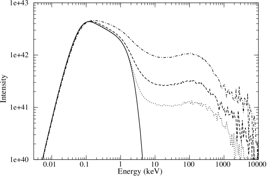
Figure 2.8: The spectrum which includes the effects of bulk motion Comptonization. Solid (Injected), dotted ($\dot{M_{h}}=0.5$), dashed ($\dot{M_{h}}=1$), dash-dotted ($\dot{M_{h}}=1.5$). $\dot{M_{d}}=1.5$ for all the cases. Keplerian disk extends up to $3.1r_{g}$. Table 2 summarizes the parameter used and the simulation results for these cases (GGCL10).

In Fig. 2.8, the emerging spectra due to the bulk motion Comptonization is shown when the halo rate is varied. The solid curve is the injected spectrum (modified blackbody). The dotted, dashed and dash-dotted curves are for $\dot{m}_{h}=0.5,\ 1$ and $1.5$, respectively. $\dot{m_{d}}=1.5$ for all the cases. The Keplerian disk extends up to $3r_{g}$. Table 2 summarizes the parameters used and the results of the simulations. As the halo rate increases, the density of the CENBOL also increases causing a larger number of scatterings. From Fig. 2.5(a), we notice that the bulk velocity variation of the electron cloud is the same for all the four cases. Hence, the case where the density is maximum, the photons got energized to a very high value due to repeated scatterings with that high velocity cold matter. As a result, there is a hump in the spectrum around 100 keV energy for all the cases. We find the signature of two power-law regions in the higher energy part of the spectrum. The spectral indices are given in Table 2. It is to be noted that $\alpha_{2}$ is increased with $\dot{m}_{h}$ and becomes softer for higher $\dot{m}_{h}$. Our geometry here at the inner edge is conical, unlike a sphere in Laurent and Titarchuk (2001). This may be the reason why our slope is not the same as in Laurent and Titarchuk (2001) where $\alpha_{2}=1.9$. In Fig. 2.9, we present the components of the emerging spectra. As in Fig. 2.7, solid curves are the spectra of all the photons that have suffered scattering. The dashed and dash-dotted curves are the spectra of photons emitted from inside and outside of the marginally stable orbit ($3r_{g}$), respectively. The photons emitted inside the marginally stable radius are Comptonized by the bulk motion of the converging infalling matter and produce the power-law tail whose spectral index is given by $\alpha_{2}$ (Table 2).

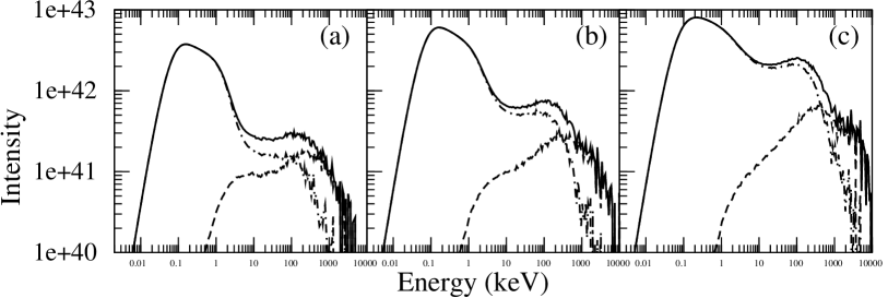
Figure 2.9: Components of the emerging spectrum for the Cases 2(a-c). Solid curves are the spectra of all the photons that have suffered some scattering. The dashed and dash-dotted curves are the spectra of photons which are emitted from inside and outside of the marginally stable orbit ($3r_{g}$) respectively. The photons emitted inside the marginally stable radius are Comptonized by the bulk motion of the infalling matter. Here the jet is absent (GGCL10).

As mentioned earlier, to compute the spectral properties of the TCAF in this Chapter, we have used the pseudo-Newtonian potential to describe the geometry around a non-rotating black hole. On the other hand, if we choose a rotating (Kerr) black hole, the space-time geometry will change which will affect the structure of the accretion disk, which in turn may affect spectral properties. Computation of topologies of global viscous transonic accretion flow has been done by Chakrabarti (1996a, 1996b) by solving the general relativistic equations and by Chakrabarti & Mondal (2006) and Mondal & Chakrabarti (2006) using pseudo-Kerr potential. These works show that in general, shock in accretion flow forms closer around rotating black holes. Thus, size of CENBOL is smaller compared to that in case of a non-rotating black hole and we expect the number of intercepted soft photons by the CENBOL to be lower. Also, the inner edge of the Keplerian disk will extend to much closer to the black hole when it is rotating for the same set of flow parameters. This may result in increase in number of soft photons, though the overall luminosity may increase. However, as the shock forms closer, post-shock region becomes hotter and may thus contribute to very high energy X-rays and gamma-rays (Chakrabarti 1996a). Therefore, as a result of all these effects, we expect overall softer spectra with powerlaw tail extending to higher energies. However, detailed study of the spectral properties from the accretion disk around a rotating black hole is necessary.

Chapter 2 SPECTRAL PROPERTIES USING TIME DEPENDENT RADIATION HYDRODYNAMIC SIMULATION

In this Chapter, we discuss the development of a time dependent radiation hydrodynamic simulation code. In this code, we couple a time dependent hydrodynamic simulation code with the Monte Carlo code described in the previous Chapter (Ghosh, Garain, Giri & Chakrabarti 2011, hereafter GGGC11; Garain, Ghosh & Chakrabarti 2012, 2013, hereaftre GGC12 and GGC13, respectively). Using this radiation hydrodynamic simulation code, we study the time variation of the hydrodynamics as well as the spectral properties of a TCAF.

3.1 Hydrodynamic simulation code

Here we present the equations which are solved in the hydrodynamic simulation code and outline the procedure to build this code. This code is an explicit, second order, finite difference code which uses the principle of total variation diminishing (TVD). Hence it is called TVD code. The TVD scheme was originally developed by Harten (1983). This code is designed to solve the hyperbolic system of conservation equations, like the conserved hydrodynamic equations. It is a nonlinear scheme obtained by first modifying the flux function and then applying a non-oscillatory first-order accurate scheme to get a resulting second order accuracy (Ryu, Brown, Ostriker & Loeb 1995 and references therein; MRC96). Thus the key merit of this scheme is to achieve the high resolution of a second-order accuracy while preserving the robustness of a non-oscillatory first-order scheme. In this code, the following time dependent hydrodynamic equations (Landau & Lifshitz 1987) are solved. In presence of gravity, these equations can be written as follows:

• Continuity equation:

  $$\frac{\partial\rho}{\partial t}+\boldsymbol{\nabla.}(\rho\boldsymbol{v})=0,$$

• Euler equation:

  $$\frac{\partial\boldsymbol{v}}{\partial t}+\boldsymbol{(v.\nabla)v}+{1\over\rho}\boldsymbol{\nabla}P=\boldsymbol{g},$$

• Energy conservation equation:

  $$\frac{\partial E}{\partial t}+\boldsymbol{\nabla.}(\boldsymbol{v}(E+P))=\rho\boldsymbol{v.g}.$$

Here, $\rho$ is the density, $\boldsymbol{v}$ is the velocity, $P$ is the pressure, $\boldsymbol{g}$ is the acceleration due to gravity and $E$ is the energy density (without potential energy) given as $E=P/(\gamma-1)+\rho v^{2}/2$, where, $\gamma$ is the polytropic index.

These equations, after some rearrangements, can be written in the vector form in cylindrical coordinate system [$R,\theta,z$] and assuming axisymmetry, as (MRC96)

$$\frac{\partial\boldsymbol{q}}{\partial t}+{1\over R}\frac{\partial(R\boldsymbol{F_{1}})}{\partial R}+\frac{\partial\boldsymbol{F_{2}}}{\partial R}+\frac{\partial\boldsymbol{G}}{\partial z}=\boldsymbol{S},$$ (3-1)

where, the state vector is

$$\boldsymbol{q}=\left(\begin{array}[]{c}\rho\\ \rho v_{R}\\ \rho v_{\theta}\\ \rho v_{z}\\ E\end{array}\right),$$

the flux functions are

$$\boldsymbol{F_{1}}=\left(\begin{array}[]{c}\rho v_{R}\\ \rho v^{2}_{R}\\ \rho v_{R}v_{\theta}\\ \rho v_{R}v_{z}\\ (E+P)v_{R}\end{array}\right),\boldsymbol{F_{2}}=\left(\begin{array}[]{c}0\\ P\\ 0\\ 0\\ 0\end{array}\right),\boldsymbol{G}=\left(\begin{array}[]{c}\rho v_{z}\\ \rho v_{R}v_{z}\\ \rho v_{\theta}v_{z}\\ \rho v^{2}_{z}+P\\ (E+P)v_{z}\end{array}\right),$$

and the source function is

$$\boldsymbol{S}=\left(\begin{array}[]{c}0\\ \frac{\rho v^{2}_{\theta}}{R}-\frac{\rho R}{2(\sqrt{R^{2}+z^{2}}-1)^{2}\sqrt{R^{2}+z^{2}}}\\ -\frac{\rho v_{R}v_{\theta}}{R}\\ -\frac{\rho z}{2(\sqrt{R^{2}+z^{2}}-1)^{2}\sqrt{R^{2}+z^{2}}}\\ -\frac{\rho(Rv_{R}+zv_{z})}{2(\sqrt{R^{2}+z^{2}}-1)^{2}\sqrt{R^{2}+z^{2}}}\\ \end{array}\right).$$

In the above equations, we have used $\boldsymbol{g}=-\boldsymbol{\nabla}\phi$, where, $\phi$ is the pseudo-Newtonian potential (PW80) given by,

$$\phi=-{1\over 2(r-1)},$$

with $r=\sqrt{R^{2}+z^{2}}$.

With the state vector $\boldsymbol{q}$ and the flux functions $\boldsymbol{F(q)=F_{1}(q)+F_{2}(q)}$ and $\boldsymbol{G(q)}$, the Jacobian matrices, $\boldsymbol{A(q)=\partial F/\partial q}$ and $\boldsymbol{B(q)=\partial G/\partial q}$ are formed. The system of equations in (3-1) are called hyperbolic if all the eigenvalues of the Jacobian matrix are real and the corresponding set of right eigenvectors is complete. The eigenvalues and the left and right eigenvectors of $\boldsymbol{A(q)}$ and $\boldsymbol{B(q)}$ are used to build the TVD code.

In updating the vector $\boldsymbol{q^{n}}$ to $\boldsymbol{q^{n+1}}$ (here $n$ represents the time step), there are two steps in this TVD code – one is the hydrodynamic step and the other is source step. In the hydrodynamic step, the eigenvectors and the eigenvalues, mentioned above, are used to compute the fluxes at the grid boundary along the $R$ and $z$ directions separately. The source terms are taken care of separately in source step. The detail procedure to build up the hydrodynamic and source steps are given in Ryu, Ostriker, Kang & Cen (1993) and Ryu et al. (1995).

3.2 Coupling of hydrodynamic and radiative transfer codes

Using the TVD code, described above, time variation of the hydrodynamical configuration of an accretion disk is simulated (MRC96; RCM97; Giri, Chakrabarti, Samanta & Ryu 2010). In order to include the effects of radiative cooling on the hydrodynamics, we couple this hydrodynamic code with the Monte Carlo code, described in the previous Chapter. So far, however, only bremsstrahlung or pseudo-Compton cooling has been added into the time-dependent flows (MSC96; CAM04; Proga 2007; Proga, Ostriker, Kurosawa 2008). Using the MC code, we compute the Comptonized spectrum from the Compton cloud. In the so called TCAF scenario (CT95), soft photons, emitted from the Keplerian disk, are intercepted and energized by the inverse-Compton scattering by the high energy electrons in the halo. In this process, the electrons lose their energy and become cooler. In the coupled code, we include the effects of this cooling and see how the hydrodynamics as well as the spectral properties of TCAF are affected because of this. In the following, we describe the procedure of coupling the hydrodynamic and Monte Carlo codes in detail (GGGC11; GGC12; GGC13).

1 Photon packet

In our simulations, soft photons are emitted from the surface of a standard Keplerian disk (SS73). We divide the Keplerian disk in different annuli of width $D(R)=0.5r_{g}$ ($r_{g}=2GM_{bh}/c^{2}$). Each annulus having mean radius $R$ is characterized by its average temperature $T(R)$. The number of photons emitted from the disk surface of each annulus can be calculated using Eq. (2-7):

$$dN(R)=4\pi RD(R)n_{\gamma}(R)\mathrm{~{}s^{-1}}.$$

The total number of photons $N$ from the whole disk surface can be computed by adding up the contributions from all the annuli. This total number $N$ is huge (e.g. $\sim~{}10^{46}$ per second for a disk extending from 3$r_{g}$ to 300$r_{g}$ and disk accretion rate $\dot{m}_{d}=0.1$). In reality, one cannot inject these many number of photons in a Monte Carlo simulation because of the limitation of computation time. So we replace the large number of photons from each annulus [$dN(R)$] by a smaller number of bundles of photons, say, $dN_{comp}(R)$ and calculate a weightage factor,

$$f_{W}=\frac{dN(R)}{dN_{comp}(R)}.$$

$dN_{comp}(R)$ is computed following the distribution function $dN(R)$. Thus each photon in the Monte Carlo simulation is assumed to be a bundle consisting of $f_{W}$ number of actual photons. All the photons in a bundle is assumed to behave in the similar way. When an injected photon is inverse-Comptonized (or, Comptonized) by an electron in a volume element of size $dV$, we assume that $f_{W}$ number of photons have suffered similar scattering with the electrons inside the volume element $dV$. If the energy loss (gain) per electron in this scattering is $\Delta E$, we multiply this amount by $f_{W}$ and distribute this loss (gain) among all the electrons inside that particular volume element. This is continued for all the $N_{comp}$ bundles of photons and the revised energy distribution is obtained. Typically, we use $N_{comp}\sim 10^{7}$ in all the simulations presented in this thesis.

2 Computation of the temperature profile after cooling

Since the hydrogen plasma considered here is ultra-relativistic ($\gamma=\frac{4}{3}$ throughout the hydrodynamic simulation), thermal energy per particle is $3k_{B}T_{e}$, where, $k_{B}$ is Boltzmann constant and $T_{e}$ is the temperature of electron. The electrons are cooled (heated up) by the inverse-Comptonization (Comptonization) of the soft photons emitted from the Keplerian disk. The protons are cooled because of the Coulomb coupling with the electrons. Total number of electrons inside any box with the center at grid location $(ir,iz)$ is given by,

$$dN_{e}(ir,iz)=4\pi rn_{e}(ir,iz)dRdz,$$

where, $n_{e}(ir,iz)$ is the electron number density at $(ir,iz)$ grid, and $dR$ and $dz$ represent the grid size along $R$ and $z$ directions, respectively. So the total thermal energy in any box is given by,

$$3k_{B}T_{e}(ir,iz)dN_{e}(ir,iz)=12\pi rk_{B}T_{e}(ir,iz)n_{e}(ir,iz)dRdz,$$

where, $T_{e}(ir,iz)$ is the temperature at $(ir,iz)$ grid. We calculate the total energy loss (gain) $\Delta E$ of electrons inside the box according to what is presented above and subtract that amount to get the new temperature of the electrons after each scattering inside that box as

$$k_{B}T_{e,new}(ir,iz)=k_{B}T_{e,old}(ir,iz)-\frac{\Delta E}{3dN_{e}(ir,iz)}.$$

3 Coupling procedure

Once a quasi steady state is achieved using the non-radiative hydro-code, we compute the radiation spectrum using the Monte Carlo code as described in the previous Chapter. This is the first approximation of the spectrum. To include the cooling in the coupled code, we follow these steps (GGGC11; GGC12; GGC13):
(i) we calculate the velocity, density and temperature profiles of the electron cloud from the output of the hydro-code.
(ii) Using the Monte Carlo code, we calculate the spectrum.
(iii) Electrons are cooled (heated up) by the inverse-Compton (Compton) scattering. We calculate the amount of heat loss (gain) by the electrons and the new temperature and energy distributions of the flow and
(iv) taking the new temperature and energy profiles as initial condition, we run the hydro-code for a time interval much shorter than the local infall time.
Subsequently, we repeat the steps (i-iv). In this way, we see how the spectrum is modified as the time proceeds. Clearly, we proceed using a two-step process. Since the calculation of Compton process is via Monte Carlo code (which is highly non-linear) while the hydrodynamic simulation is by finite difference method, they cannot be coupled directly.

Before proceeding further, we first show that our choice of $N_{comp}~{}\sim~{}10^{7}$ produces converging results. Before the choice of $N_{comp}~{}\sim~{}10^{7}$ was made, we varied $N_{comp}$ from $\sim 10^{3}$ to $\sim 1.5\times 10^{7}$ and conducted a series of runs to ensure that our final result does not suffer from any statistical effects. Fig. 3.1 shows the average electron temperature of the cloud when $N_{comp}$ was varied. There is a clear convergence in our result for $N_{comp}>6\times 10^{6}$ (see also, GGC12).

As mentioned earlier, we model soft photons emitted from Keplerian disks using $\rm{N_{comp}}$. As the disk rate is increased, number of soft photons increases and to model higher number of photons, we need higher value of $\rm{N_{comp}}$. In the present work, we have shown that $\rm{N_{comp}}>6\times 10^{6}$ models the number soft photons emitted for the higher disk rates (Cases C and D) very well. Therefore, it is evident that this result will remain valid for lower values of disk rates also (i.e., for other cases presented in Table 3). For this reason, we have shown the temperature convergence results for cases C and D only. However, we conducted more tests in GGC12 and there we showed similar results for other disk rates. Thus, we believe that using the value $\rm{N_{comp}}\sim 10^{7}$ will produce correct results for moderate disk rates ($\sim$ 1 or lower).

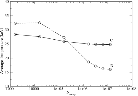
Figure 3.1: Variation of the average temperature (keV) of the electron cloud with bundle of photons $N_{comp}$ for two different Keplerian disk rates $\dot{m}_{d}$, keeping the halo rate fixed at $\dot{m}_{h}=0.5$. Simulation cases (Table 3) are marked on each curve. Clearly, the temperature converges for $N_{comp}>6\times 10^{6}$ (see also, GGC12).

3.3 Spectral properties of TCAF using coupled code

We study the spectral properties of the TCAF using the coupled radiation hydrodynamic simulation code. In Fig. 3.2, we present the schematic diagram of the simulation set up (see also, GGGC11).

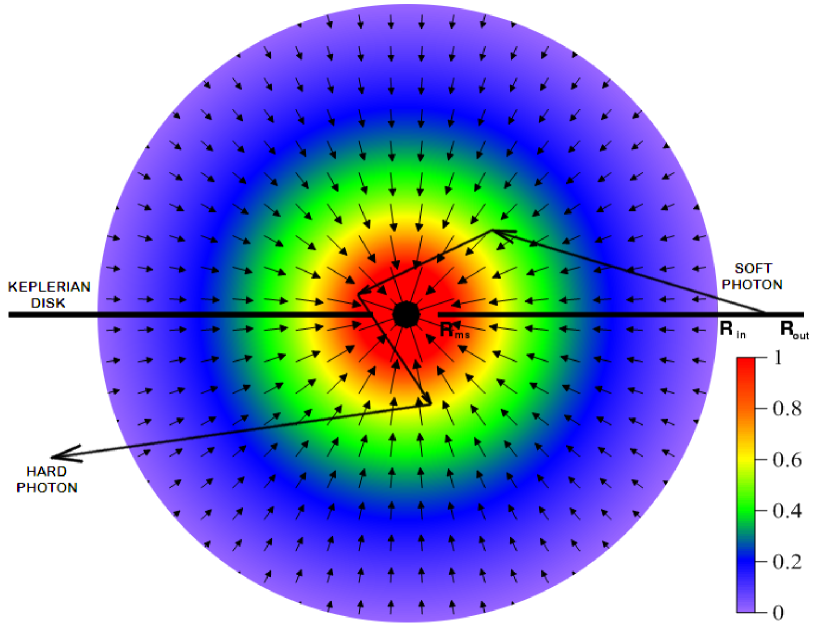
Figure 3.2: Schematic diagram of the geometry of our Monte Carlo simulations for $\lambda=0$. The colors show the normalized density in a logarithmic scale. Velocity vectors of the infalling electrons are also shown. The zig-zag trajectory is the typical path followed by a photon inside the cloud (see also, GGGC11).

We consider a spherically symmetric Compton cloud (halo) with zero angular momentum (specific angular momentum $\lambda=0$) within a sphere of radius $R_{in}=200r_{g}$. The Keplerian disk resides at the equatorial plane. The outer edge of this disk is located at $R_{out}=300r_{g}$ and it extends inside up to the marginally stable orbit $R_{ms}=3r_{g}$. At the centre of the sphere, a non-rotating black hole of mass $10M_{\odot}$ is kept. The matter is injected with spherical symmetry from the radius $R_{in}$. It intercepts the soft photons emerging out of the Keplerian disk and reprocesses them via Compton or inverse-Compton scattering.

1 Density, velocity and temperature profiles inside the halo component

A realistic accretion disk is three-dimensional. Assuming axisymmetry, we reduce the problem to two dimensions and solve the hydrodynamic equations, written in two dimensions, numerically to simulate the accretion flow of the halo. The flow dynamics is calculated using the TVD code (discussed in the earlier Section). At each time step, we carry out Monte Carlo simulation to obtain the cooling/heating due to Comptonization. We incorporate the cooling/heating of each grid while executing the next time step of hydrodynamic simulation, as discussed above. The numerical calculation for the two-dimensional flow has been carried out with $900\times 900$ equi-spaced cells in a $200r_{g}\times 200r_{g}$ box (GGGC11). We choose the units in such a way that the outer boundary ($R_{in}$) is chosen to be unity and the matter density is normalized to become unity. We assume the black hole to be non-rotating and we use the pseudo-Newtonian potential $-\frac{1}{2(r-1)}$ (PW80) to calculate the flow geometry around the black hole ($r$ is in $r_{g}$).

Figure 3.3: (a) Density and (b) temperature contours inside the spherically accreting halo in the absence of Compton cooling. Here, densities are in normalized units and temperatures are in keV (GGGC11). The radial variation of the velocity profile is also shown in (c). See text for details.

In Figs 3.3(a-b), we show the snapshots of the normalized density and temperature (in keV) profiles obtained in a steady state purely from our hydrodynamic simulation. The density contour levels are drawn for $0.65-1.01$ (levels increasing by a factor of $1.05$) and $1.01-66.93$ (levels increasing by a factor of $1.1$). The temperature contour levels are drawn for $16.88-107.8$ keV (levels increasing by a factor of $1.05$). The radial variation of the velocity profile is also shown in Fig. 3.3(c). The velocity is measured in the unit of $c$. As it is seen from 3.3(c), the velocity $v\to c$ as $r\to 1$ (event horizon) and that makes it important to consider gravity effects (light bending, redshift etc.) on emerging photon. For the present simulations, we have taken into account the effect of redshift, although the effects of light bending has not been taken into consideration. However, we are in the process to improve the code by cosidering the gravity effects as much as possible and in this regard, we have discussed the computational procedure to compute photon trajectory in Schwarzschild geometry in Appendix A.

2 Keplerian disk

We assume a steady Keplerian disk and use the standard Shakura-Sunyaev disk (SS73) as the source of soft photons for this case. The Keplerian disk is placed on the equatorial plane. For the present simulations, we neglect the reflection and/or absorption of photons by the Keplerian disk (GGGC11; GGC12; GGC13).

The radial variations of the disk temperature and number of generated photons are given in Eq. (1) and (2-7), respectively. In the Monte Carlo simulation, we incorporated the directional effects of photons coming out of the Keplerian disk with the maximum number of photons emitted in the $z$-direction and minimum number of photons are generated along the plane of the disk (GGGC11). Thus, in the absence of photon bending effects, the disk is invisible as seen edge on. The position of each emerging photon is randomized using the distribution function given by Eq. (2-7).

3 Simulation procedure

The spectral properties are studied using the coupled radiation hydrodynamic simulation code, described in the previous Section. For a particular simulation, we assume a Keplerian disk rate ($\dot{m}_{d}$) and a halo rate ($\dot{m}_{h}$). The specific energy ($\epsilon$) of the halo provides the hydrodynamic (e.g., number density of the electrons and the velocity distribution) and the thermal properties of matter.

Before beginning the coupled code simulation, we simulate a steady state flow profile using the non-radiative hydro code (RCM97; Giri et al. 2010). This steady state flow is used as the initial condition for the coupled simulation run. On this flow profile, we start the Monte Carlo simulation. The simulation procedure of the Monte Carlo part is exactly same as that is described in Section 2.1. When a photon interacts with an electron via Compton or inverse-Compton scattering, it loses or gains some energy ($\Delta E$). At each grid point, we compute $\Delta E$ (PSS83). We update the energy of the flow at this grid by this amount and continue the hydrodynamic code with this modified energy. This, in turn, modify the hydrodynamic profile. In case the final state is steady, the temperature of the cloud would be reduced progressively to a steady value from the initial state where no cooling was assumed. If the final state is oscillatory, the solution would settle into a state with Comptonization.

4 Results and discussions

In Table 3, we summarize all the cases for which the simulations have been presented in this Chapter. Similar cases have been presented for different sets of parameters in GGGC11. In Column 1, various case IDs are marked. Column 2 shows the specific energy ($\epsilon$) of the halo at the outer boundary. The Keplerian disk rate ($\dot{m}_{d}$) and the sub-Keplerian halo rate ($\dot{m}_{h}$) are listed in Columns 3 and 4. The number of soft photons, injected from the Keplerian disk ($N_{inj}$) for various disk rates, can be found in Column 5. Column 6 lists the number of photons ($N_{sc}$) that have suffered at least one scattering inside the electron cloud. The number of photons ($N_{unsc}$), escaped from the cloud without any scattering are listed in Column 7. Columns 8 and 9 give the percentages of injected photons that have entered into the black hole ($N_{bh}$) and suffered scattering ($p=\frac{N_{sc}}{N_{inj}}$), respectively. The cooling time ($t_{0}$) of the system is defined as the expected time for the system to lose all its thermal energy with the particular flow parameters (namely, $\dot{m}_{d}$ and $\dot{m}_{h}$). We calculate $t_{0}=E/{\dot{E}}$ in each time step, where, $E$ is the total energy content of the system and ${\dot{E}}$ is the energy gain or loss by the system in that particular time step and present it in Column 10. We present the energy spectral index $\alpha,~{}[I(E)\sim E^{-\alpha}]$ obtained from our simulations in the last column.

Table 3: Parameters used for the simulations and a summary of results.
Case	$\epsilon$	$\dot{m}_{d}$	$\dot{m}_{h}$	$N_{inj}$	$N_{sc}$	$N_{unsc}$	$N_{bh}$ (%)	$p$ (%)	$t_{0}$ (s)	$\alpha$
A	22e-4	1e-4	0.5	7.1e+41	9.6e+40	6.1e+41	0.184	13.511	196.4	1.41, 0.91
B	22e-4	1e-3	0.5	4.0e+42	5.4e+41	3.5e+42	0.186	13.5	24.4	1.44, 0.75
C	22e-4	1e-2	0.5	2.3e+43	3.1e+42	2.0e+43	0.179	13.351	4.0	1.61, 0.66
D	22e-4	1e-1	0.5	1.2e+44	1.5e+43	1.1e+44	0.149	12.683	0.2	2.11, 0.53
E	22e-4	1e-3	1	4.0e+42	9.8e+41	3.0e+42	0.327	24.377	6.0	1.15
F	22e-4	1e-3	2	4.0e+42	1.6e+42	2.4e+42	0.608	40.636	1.2	0.85
G	22e-4	1e-3	5	4.0e+42	2.7e+42	1.3e+42	1.224	66.507	0.2	0.52

Figure 3.4: Changes in the density distribution in presence of cooling. $\dot{m}_{h}=0.5$ for all the cases. Disk accretion rates $\dot{m}_{d}$ used are (a) $10^{-4}$, (b) $10^{-3}$ and (c) $10^{-2}$, respectively (Cases A-C of Table 3). The density contours are drawn using the same contour levels as in Fig. 3.3(a) (see also, GGGC11).

Figure 3.5: Changes in the temperature distribution in presence of cooling. $\dot{m}_{h}=0.5$ for all the cases. Disk accretion rates $\dot{m}_{d}$ are (a)$10^{-4}$, (b)$10^{-3}$ and (c)$10^{-2}$, respectively (Cases A-C of Table 3). Contours are drawn using the same levels as in Fig. 3.3(b) (see also, GGGC11).

In Figs 3.4(a-c), we present the changes in density distribution as the disk accretion rates are changed: $\dot{m}_{d}=$ (a) $10^{-4}$, (b) $10^{-3}$ and (c) $10^{-2}$, respectively. We notice that as the accretion rate of the disk is enhanced, the density distribution losses its spherical symmetry (see also, GGGC11). In particular, the density at a given radius is enhanced in a conical region along the axis. This is due to the cooling of the matter by Compton scattering. To show this, in Figs 3.5(a-c), we show the contours of constant temperatures (marked on curves) for the same three cases. We notice that the temperature is reduced along the axis (where the optical depth as seen by the soft photons from the Keplerian disk is higher) drastically after repeated Compton scatterings.

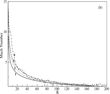
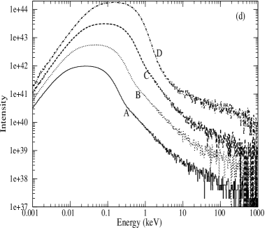
Figure 3.6: (a) Sonic surfaces at different stages of iterations. The outermost curve represents the final converged solution (see also, GGGC11). The initial spherical sonic surface become prolate spheroid due to cooling by the Keplerian disk at the equatorial plane. Parameters are for Case C (Table 3). (b) Mach number variation as a function of distance after a complete solution of the radiative flow is obtained. Plot no. 1 corresponds to the solution from adiabatic Bondi flow. Plots 2-4 are the solutions along the equatorial plane, the diagonal and the axis of the disk, respectively (see also, GGGC11). Parameters are for Case C (Table 3). (c) Variation of the average temperature of the Compton cloud as the iteration proceeds when the disk accretion rate is varied keeping the halo rate constant at $\dot{m}_{h}=0.5$. The solid, dotted, dashed and dash-dotted plots are for $\dot{m}_{d}=0.0001$, $0.001$, $0.01$ and $0.1$ respectively. Case numbers (Table 3) are marked. With the increase of disk rate, the temperature of the Compton cloud converges to a lower temperature (see also, GGGC11). (d) Variation of the spectrum with the increase of disk accretion rate. Parameters are the same as in (c). With the increase in $\dot{m}_{d}$, the intensity of the spectrum increases due to the increase in $N_{inj}$ (see, Table 3). The spectrum is softer for higher values of $\dot{m}_{d}$ (see also, GGGC11). The spectral slope for each of these spectra is listed in Table 3.

In Figs 3.6(a-d), we show the hydrodynamic and radiative properties. In Fig. 3.6(a), we show the sonic surfaces. The lowermost curve corresponds to theoretical solution for an adiabatic flow (e.g., C90). Other curves from the bottom to the top are the iterative solutions for the Case C mentioned above. As the disk rate is increased, the cooling increases, and consequently, the Mach number increases along the axis (see also, GGGC11). Of course, there are other effects: the cooling causes the density to go up to remain in pressure equilibrium. In Fig. 3.6(b), the Mach number variation is shown. The lowermost curve (marked 1) is from the theoretical consideration. Plots marked 2-4 are the variation of Mach number with radial distance along the equatorial plane, along the diagonal and along the vertical axis respectively (see also, GGGC11). In Fig. 3.6(c), the average temperature of the spherical halo is plotted as a function of the iteration time until almost steady state is reached. The cases are marked on the curves. We note that as the injection of soft photons increases, the average temperature of the halo decreases drastically (see also, GGGC11). In Fig. 3.6(d), we plot the energy dependence of the photon intensity. We find that, as we increase the disk rate, keeping the halo rate fixed, number of photons coming out of the cloud in a particular energy bin increases and the spectrum becomes softer (see also, GGGC11). This is also clear from Table 3; $N_{inj}$ increases with $\dot{m}_{d}$, increasing $\alpha$. We find the signature of double slopes in these cases. As the disk rate increases, the second slope becomes steeper. This second slope is the signature of bulk motion Comptonization (CT95). As $\dot{m}_{d}$ increases, the cloud becomes cooler [Fig. 3.6(c)] and the power-law tail due to the bulk motion Comptonization (CT95; Chakrabarti 1997; GGCL10; GGGC11) becomes prominent.

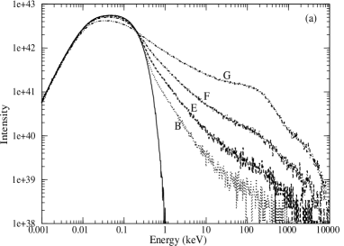
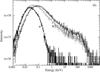
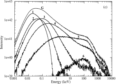
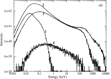
Figure 3.7: (a) Variation of the spectrum with the increase of the halo accretion rate, keeping the disk rate ($\dot{m}_{d}=0.001$) fixed. The dotted, dashed, dash-dotted and double dot-dashed curves show the spectra for $\dot{m}_{h}=0.5$, $1$, $2$ and $5$ respectively. The injected multicolor blackbody spectrum supplied by the Keplerian disk is shown by solid line (see also, GGGC11). (b) Directional dependence of the spectrum: $\dot{m}_{h}=5$, $\dot{m}_{d}=0.001$ are the flow parameters. The solid, dotted and dashed curves are for observing angles $2^{\circ}$, $45^{\circ}$ and $90^{\circ}$ respectively (see also, GGGC11). All the angles are measured with respect to the rotation axis ($z$-axis). Intensity of spectra emerging from the cloud after suffering various number of scatterings (c) and at four different times (d) immediately after the injection of soft photons. Case G is assumed. The spectra of the photons suffering 0, 1, 2-3, 4-7, 8-15 and more than 16 scatterings are shown by the plots marked as 1, 2, 3, 4, 5 and 6 (Fig. 3.7c) respectively, within the cloud. Curve G is the net spectrum for which these components are drawn. As the number of scattering increases, the photons gain more and more energy from the hot electron cloud through inverse-Comptonization process (see also, GGGC11). The spectra of the photons spending 0.01-20, 20-40, 40-100 and more than 100 ms time inside the electron cloud are marked by 1, 2, 3 and 4 (Fig. 3.7d) respectively (see also, GGGC11).

In Fig. 3.7(a), we show the variation of the energy spectrum with the increase of the halo accretion rate, keeping the disk rate fixed ($\dot{m}_{d}=0.001$). The injected multi-color blackbody spectrum supplied by the Keplerian disk is shown (solid line). The dotted, dashed, dash-dotted and double dot-dashed curves show the spectra for $\dot{m}_{h}=0.5$, $1$, $2$ and $5$, respectively. The spectrum becomes harder for higher values of $\dot{m}_{h}$ as it is difficult to cool a higher density matter with the same number of injected soft photons (CT95; GGGC11). In Fig. 3.7(b), we show the directional dependence of the spectrum for $\dot{m}_{h}=5$, $\dot{m}_{d}=0.001$ (Case G). The solid, dotted and dashed curves are for observing angles (a) $2^{\circ}$, (b) $45^{\circ}$ and (c) $90^{\circ}$ respectively. All the angles are measured with respect to the rotation axis ($z$-axis). As expected, the photons arriving along the z-axis would be dominated by the soft photons from the Keplerian disk while the power-law would dominate the spectrum coming edge-on (see also, GGGC11). We now study the dependence of the spectrum on the residence time of an injected photon inside the cloud. Depending on the number of scattering suffered and the length of path traveled, different photons spend different times inside the Compton cloud (GGGC11). The energy gain or loss by any photon depends on this time. Fig. 3.7(c) shows the spectrum of the photons suffering different number of scatterings inside the cloud. Here, counts marked as 1, 2, 3, 4, 5 and 6 show the spectrum for 6 different ranges of number of scatterings. Plot 1 shows the spectrum of the photons that have escaped from the cloud without suffering any scattering. This spectrum is as same as the injected spectrum, only difference is that it is Doppler shifted. As the number of scattering increases (spectrum 2, 3 and 4), the photons are more and more energized via inverse-Compton scattering with the hot electron cloud. For scatterings more than 8, the high energy photons start loosing energy through Compton scattering with the relatively lower energy electrons (see also, GGGC11). Components 5 and 6 show the spectra of the photons suffering 8-15 scatterings and the photons suffering more than 16 scatterings respectively. Here the flow parameters are: $\dot{m}_{d}=0.001$ and $\dot{m}_{h}=5$ (Case G, Table 3).

In Fig. 3.7(d), we plot the spectrum emerging out of the electron cloud at four different time ranges. In the simulation, the photons take $0.01$ to $150$ ms to come out of the system. We divide this time range into 4 suitable bins and plot their spectrum. Case G of Table 3 is considered. We observe that the spectral slopes and intensities of the four spectra are different. As the photons spend more and more time inside the cloud, the spectrum gets harder (plots 1, 2 and 3). However, very high energy photons which spend maximum time inside the cloud lose some energy to the relatively cooler electrons before escaping from the cloud. Thus the spectrum 4 is actually the spectrum dominated by the Comptonized photons (see also, GGGC11).

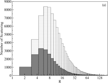
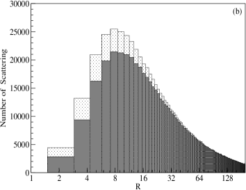
Figure 3.8: Number of scatterings inside the spherical shell between $R$ to $R+\delta R$ ($\delta R\sim 1.4$). The light and dark shaded histograms are for the cloud with and without bulk velocity, respectively (see also, GGGC11). (a) Only the photons emerging from the cloud with energies $E$, where $50$ keV $<E<150$ keV, are considered here. (b) All the photons emerging from the cloud are considered here. Parameters used: $\dot{m}_{d}=0.001$ and $\dot{m}_{h}=5$ (Case G Table 3).

We observe that the emerging spectrum has a bump, especially at higher accretion rates of the halo, at around $100$ keV (e.g., the spectra marked F, G in Fig. 3.7(a)). A detailed analysis of the emerging photons having energies between 50 to 150 keV was made to see where in the Compton cloud these photons were produced (GGGC11). In Fig. 3.8(a), we present the number of scatterings inside different spherical shells within the electron cloud suffered by these photons ($50<E<150$ keV) before leaving the cloud. Parameters used: $\dot{m}_{d}=0.001$ and $\dot{m}_{h}=5$. The light and dark shaded histograms are for the cloud with and without bulk velocity components, respectively. We find that the presence of bulk motion of the infalling electrons pushes the photons towards the hotter and denser [Figs 3.3(a-b)] inner region of the cloud to suffer more and more scatterings (GGGC11). We find that the photons responsible for the bump suffered maximum number of scatterings at around $8r_{g}$. From the temperature contours, we find that the cloud temperature around $8r_{g}$ is $\sim 100$ keV. This explains the existence of the bump. In Fig. 3.8(b), we consider all the outgoing photons independent of their energies. The difference between the two cases is not so visible. This shows that the bulk velocity contributes significantly to produce the highest energy photons.

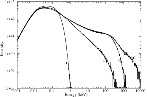
Figure 3.9: The spectrum for the Case G. The curves marked 2 and 3 give the spectra when the bulk velocity of the electron is absent for the whole cloud and for the cloud inside $3r_{g}$, respectively. The curve marked 1 gives the injected spectrum. The bulk motion Comptonization of the photons inside the $3r_{g}$ radius creates the hard tail. The bump near 100 keV is due to a combined effect of the temperature and bulk velocity of the rest of the cloud (see also, GGGC11).

In Fig. 3.9, we explicitly show the effects of the bulk velocity on the spectrum. We note that the bump disappears when the bulk velocity of the electron cloud is chosen to be zero (Curve marked 2). This fact shows that the region around $8r_{g}$ in presence of the bulk motion behaves more like a blackbody emitter, which creates the bump in the spectrum (see also, GGGC11). Since the photons are suffering a large number of scatterings near this region ($8r_{g}$), most of them emerge from the cloud with the characteristic temperature of the region. The effect of bulk velocity in this region is to force the photons to suffer larger number of scatterings (GGGC11). This bump vanishes for lower density cloud (low $\dot{m}_{h}$) as the photons suffer lesser number of scatterings. The photons which are scattered close to the black hole horizon and escape without any further scattering, produce the high energy tail in the output spectrum. Curve 3 of Fig. 3.9 shows the intensity spectrum of Case G (Table 3), when there are zero bulk velocity inside $3r_{g}$. We find that in the absence of bulk velocity inside $3r_{g}$, the high energy tail in the Curve G vanishes. This is thus a clear signature of the presence of bulk motion Comptonization near the black hole horizon (CT95; Chakrabarti 1997; GGGC11).

Chapter 3 EFFECTS OF COMPTON COOLING ON OUTFLOWS

The winds and jets in a compact binary system containing black holes are generally believed to be originated from the disk itself (C96; C99; Das et al. 2001; Das & Chattopadhyay 2008). There are several hydrodynamical models of the formation of outflows from the disks ranging from the twin-exhaust model of Blandford & Rees (1974), to the self-similar models of Blandford & Payne (1982) and Blandford & Begelman (1999). Assuming that the outflows are transonic in nature, Fukue (1983) and Chakrabarti (1986) computed the velocity distribution without and with rotational motion in the flow and showed that the flow could become supersonic close to the black hole. Camenzind and his group extensively worked on the magnetized jets and showed that the acceleration and collimation of the jets could be achieved (e.g., Appl & Camenzind 1993). In a subsequent two component transonic flow model, CT95 pointed out that the jets could be formed only from the inner part of the disk i.e., the CENBOL.

While the general picture of the outflow formation is thus understood and even corroborated by the radio observation of the base of the powerful jet, such as in M87 (Junor, Biretta & Livio 1999), that the base of the jet is only a few tens of $r_{g}$, a major question still remained: what fraction of the matter is driven out from the disk and what are the flow parameters on which this fraction depends? In a numerical simulation using SPH code, MLC94 showed that the outflow rates from an inviscid accretion flow strongly depends on the outward centrifugal force and 15-20 percent matter can be driven out of the disk. Chakrabarti (1998c), C99, Das et al. (2001), Chattopadhyay, Das & Chakrabarti (2004) estimated the ratio of the outflow rate to the inflow rate analytically and found that the shock strength determines the ratio. For very strong and very weak shocks, the outflow rates are very small, while for the shocks of intermediate strength, the outflow rate is significant. This is in line with the observations (Gallo, Fender & Pooley 2004; Fender, Belloni, Gallo 2004; Fender, Gallo & Russell 2010) that the spectrally soft states have less outflows.

In this Chapter, we concentrate on the formation of outflows from the accretion disk around black holes by numerical simulation and study the effects of Compton cooling on it using the time dependent radiation hydrodynamic simulation code (GGC12). While computing the time variation of the velocity components, density and temperature, we also compute the temporal dependence of the spectral properties. As a result, not only we compute the outflow properties, we correlate them with the spectral properties (GGC12). Not surprisingly, we find that whenever the Compton cloud or the CENBOL is cooled down and the spectrum becomes softer, the outflow, originating from CENBOL, losses its drive and its rate is greatly reduced. In the following, we discuss the simulation procedure and the results of our study. Same conclusions are found in GGC12 where simulations are done using different sets of input parameters on similar simulation set up.

4.1 Simulation set up

In Fig. 4.1, we present the schematic diagram of our simulation set up for the Compton cloud with a specific angular momentum $\lambda=1.75$ (see also, GGC12). The sub-Keplerian matter enters the simulation box through the outer boundary at $R_{in}=100r_{g}$ ($r_{g}=2GM_{bh}/c^{2}$). The Keplerian disk resides at the equatorial plane of the cloud. The outer edge of this disk is assumed to be at $R_{out}=200r_{g}$ and it extends inside up to the marginally stable orbit $R_{ms}=3r_{g}$. At the centre, a non-rotating black hole of mass $M_{bh}=10M_{\odot}$ is located. The soft photons emerging out of the Keplerian disk are intercepted and reprocessed via Compton or inverse-Compton scattering by the sub-Keplerian matter. An injected photon may undergo no scattering at all or a single or multiple scatterings with the hot electrons in between its emergence from the Keplerian disk and its escape from the sub-Keplerian halo. The photons which enter the black hole are absorbed.

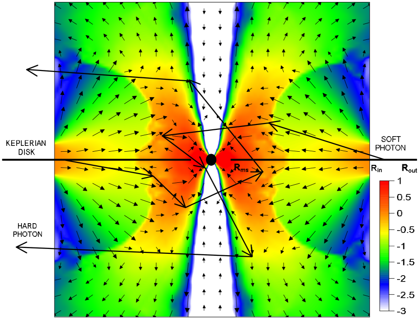
Figure 4.1: Schematic diagram of the geometry of our Monte Carlo simulations. The colors represent the normalized density in logarithmic scale. The zig-zag trajectories are the typical paths followed by the photons. The velocity vectors of the infalling matter inside the cloud are shown. The velocity vectors are plotted for $\lambda=1.75$ (see also, GGC12).

1 Density, velocity and temperature profiles inside the halo component

The inflowing halo matter has some angular momentum with respect to the black hole. Therefore, as it approaches the black hole, the outward centrifugal force becomes comparable to the gravitational force at acertain radius. As a result, the matter slows down and we find the formation of shocks in the incoming supersonic flow (Chakrabarti 1989a,b; C90). Subsequently, the matter accelerates and becomes supersonic again as it approaches the black hole. In the post-shock region, the density and the temperature of the halo increases to much higher value. This region is the CENBOL of the TCAF model (CT95).

Assuming axisymmetry, we calculate the flow dynamics using the TVD code in a similar way as described in the previous Chapter. At each time step, we carry out Monte Carlo simulation to obtain the cooling/heating due to Comptonization. We incorporate the cooling/heating of each grid while executing the next time step of hydrodynamic simulation. For the present case, the numerical simulation for the two-dimensional flow has been carried out with $512\times 512$ equi-spaced cells in a $100r_{g}\times 100r_{g}$ box (GGC12; GGC13). We choose the units in a way that the outer boundary ($R_{in}$) is unity and the matter density at the outer boundary is also normalized to unity (MRC96; Giri et al. 2010; GGGC11). We assume the black hole to be non-rotating and we use the pseudo-Newtonian potential $-\frac{1}{2(r-1)}$ (PW80) to calculate the flow geometry around a black hole.

4.2 Simulation procedure

All the simulations have been carried out using the time dependent radiation hydrodynamic simulation code described in the previous Chapter. Before starting the simulation, we generated a steady state flow profile using the non-radiative hydro code. This steady state is used as the initial condition for the radiation hydrodynamic simulation (GGGC11; GGC12). The Keplerian disk at the equatorial plane supplies soft photons. These photons interact with the high energy electrons of the halo and they exchange their energy through Compton or inverse-Compton scattering.

We use a standard Keplerian disk (SS73) as the source of soft photons. The emission is of blackbody type characterized by the local surface temperature. The radial variations of the surface temperature and the number of generated photons from the disk surface are given in Eq. (1) and (2-7), respectively. We also incorporate the directional effects as described in Chapter 3. In these simulations, we neglect the reflection and/or absorption of the soft photons by the Keplerian disk.

For a particular simulation, we use the Keplerian disk rate ($\dot{m}_{d}$) and the sub-Keplerian halo rate ($\dot{m}_{h}$) as parameters. The specific energy ($\epsilon$) and the specific angular momentum ($\lambda$) determine the hydrodynamics (shock location, number density and velocity variations etc.) and the thermal properties of the sub-Keplerian matter (GGC12; GGC13). We assume the absorbing boundary condition at $r=1.5$ since any inward pointing photon at that radius would be sucked into the black hole.

4.3 Results and discussions

Table 4: Parameters used for the simulations.
Case	$\epsilon,\lambda$	$\dot{m}_{h}$	$\dot{m}_{d}$
Ia	0.0021, 1.80	0.1	No Disk
Ib	0.0021, 1.80	0.1	1e-4
Ic	0.0021, 1.80	0.1	2e-4
Id	0.0021, 1.80	0.1	5e-4
IIa	0.0021, 1.75	0.1	No Disk
IIb	0.0021, 1.75	0.1	1e-4
IIc	0.0021, 1.75	0.1	2e-4
IId	0.0021, 1.75	0.1	5e-4

In Table 4, we list various Cases with all the simulation parameters used in this Chapter. The specific energy ($\epsilon$) and specific angular momentum ($\lambda$) of the sub-Keplerian halo at the outer boundary are given in Column 2. These parameters are chosen from the region of the parameter space for which shock formation is possible in an accretion flow in vertical equilibrium (Chakrabarti & Das 2001). Columns 3 and 4 give the halo ($\dot{m}_{h}$) and the disk ($\dot{m}_{d}$) accretion rates. The corresponding cases are marked in Column 1. In Cases Ia and IIa, no Keplerian disk was placed in the equatorial plane of the halo. These are non-radiative hydrodynamical simulations and no Compton cooing is included. To show the effects of Compton cooling on the hydrodynamics of the flow, the Cases I(b-d) and II(b-d) are run till the same time as the Cases Ia and IIa (GGC12).

All of the simulations, presented in this Chapter, have been run for $\sim$ 2 sec. For these cases, the time averaged values of the infall time scale for the matter is found to be $\sim$ 0.12 s for $\lambda=1.80$ cases and $\sim$ 0.1 s for $\lambda=1.75$ cases. These numbers have been computed from the numerical simulation results. Therefore, it is seen that the simulations have been run for $\sim$ 20 dynamical times. It can be seen that accretion flow configuration reaches the equilibrium in about 0.1 s and the flow does not change if the accretion rate parameters are not changed with time. Thus, we believe that all the results are the stable.

1 Properties of the shocks in presence of cooling

Figure 4.2: The variation of shock location (in $r_{g}$) at the equatorial plane with time (in sec) for different Keplerian disk rates $\dot{m}_{d}$, keeping the halo rate fixed at $\dot{m}_{h}=0.1$. Simulation Cases are marked on each curve. (a) $\lambda=1.80$ and (b) $\lambda=1.75$. Cooling decreases the average shock location (see also, GGC12).

In Figs 4.2(a) and (b), we present the time variation of the shock location (in units of $r_{g}$) for various Cases (marked on each curve) given in Table 4. All the solutions exhibit oscillatory shocks. For no cooling, the higher angular momentum produces shocks at a higher radius, which is understandable, since the shock is primarily centrifugal force supported. However, as the cooling is increased the average shock location decreases since the cooling reduces the post-shock thermal pressure and the shock could not be sustained till higher thermal pressure is achieved at a smaller radius. The corresponding oscillations are also suppressed. The average shock location is found to be almost independent of the specific angular momentum at this stage (see also, GGC12).

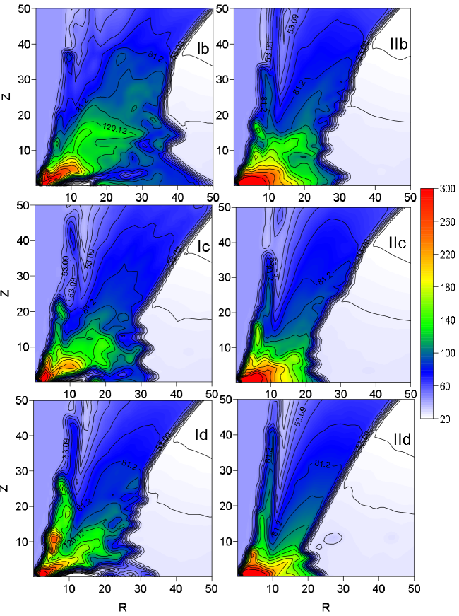
Figure 4.3: Colour map of final temperature distributions in the region ($50r_{g}\times 50r_{g}$) of the accretion disk for different disk rates are shown. The left panel is for $\lambda=1.80$ and the right is for $\lambda=1.75$. As $\dot{m}_{d}$ is increased, we find that, the high temperature region (dark red) shrinks (see also, GGC12).

In Fig. 4.3, we show the colour map of the temperature distribution at the end of our simulation. We zoomed the region $50r_{g}\times 50r_{g}$. The specific angular momentum is $1.80$ in the left panel and $1.75$ in the right panel. Cases are marked. We note the collapse of the post-shock region as $\dot{m}_{d}$ is increased gradually (see also, GGC12).

Figure 4.4: Variation of the average temperature (keV) of the post shock region with time (sec) for different Keplerian disk rates $\dot{m}_{d}$, keeping the halo rate fixed at $\dot{m}_{h}=0.1$ (see also, GGC12). Parameters are the same as in Figs 4.2(a) and (b).

We take the post-shock region in each of these cases, and plot in Figs 4.4(a) and (b) the average temperatures of the post-shock region only for those cases where the cooling due to Comptonization is included. The average temperature was obtained by the optical depth weighted averaging procedure prescribed in CT95. The average temperature in the post-shock region is reduced rapidly as the supply of the soft photons is increased (see also, GGC12).

2 Effects of Comptonization on the outflow

We now concentrate on how the outflow rate is affected by the Comptonization. Outflows move to very large distances and thus must not be bound to the system, i.e., the specific energy should be positive. Matter should also be of higher entropy as it is likely to be relativistic. Because of this, we wish to concentrate on the behaviour of matter which have highest energy and entropy (GGC12). Though we injected matter at the outer edge with a constant specific energy, the energy of matter in the post-shock region is redistributed due to turbulence, Compton cooling and shock heating. Some entropy is generated as well. The high energy and high entropy matter escape in the form of a hollow cone around the axis. It is thus expected that if the post-shock region itself is collapsed due to Comptonization, the outflows will also be quenched (GGC12). We show this effect in our result below.

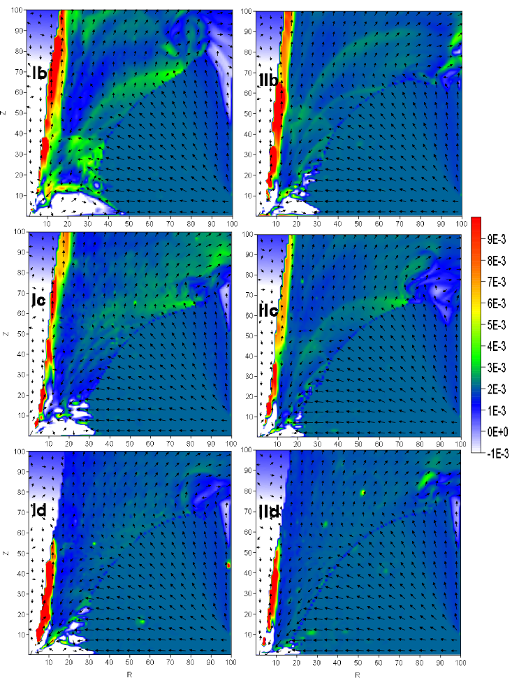
Figure 4.5: Colour map of final specific energy distribution inside the accretion disk for different disk rates. The high energy matter (dark red) are ejected outward as a hollow jet. The matter with a high energy flow decreases with the increase in disk rate. Velocity vectors at the injection boundary on the right is of length $0.05$ (see also, GGC12).

In Fig. 4.5, we present the specific energy distribution for both the specific angular momenta (left panel for $\lambda=1.80$ and right panel for $\lambda=1.75$) for all the cooling Cases (marked in each box) at the end of our simulation. The velocity vectors are also plotted. The scale on the right gives the specific energy. First we note that the jets are stronger for higher angular momentum. This is because the post-shock region (between the shock and the inner sonic point close to the horizon) is hotter. Second, lesser and lesser amount of matter has higher energy as the cooling is increased (see also, GGC12).

Figure 4.6: Color map of the final entropy ($K=\frac{P}{\rho^{\gamma}}$) distribution. Other parameters are as in Fig. 4.5. The high entropy flow decreases as the disk rate increases (see also, GGC12).

A similar observation could be made from Fig. 4.6, where the entropy distribution is plotted. The jet matter having upward pointing vectors have higher entropy. However, this region shrinks with the increase in Keplerian rate, as the cooling becomes significant the outward thermal drive is lost (GGC12). Here, the velocity vectors are of length $0.05$ at the outer boundary on the right and others are scaled accordingly.

In order to quantify the decrease in the outflow rates with cooling, we define two types of outflow rates (GGC12). One is $\dot{M}_{out}$ which is defined to be the rate at which the outward pointing flow leaves the computational grid. This will include both the high and low energy components of the flow.

Figure 4.7: Variations of $R_{\dot{m}}(=\frac{\dot{M}_{out}}{\dot{M}_{in}})$ with time for different $\dot{m_{d}}$ are shown here. (a) $\lambda=1.80$ and (b) $\lambda=1.75$. The Cases are marked in each panel. The outflow rate is the lowest for the highest Keplerian disk accretion rate (Cases are Id and IId) (see also, GGC12).

In Figs 4.7(a) and (b), we show the results of time variation of the ratio $R_{\dot{m}}$ (${\dot{M}}_{out}$ / ${\dot{M}}_{in}$) for the four cases (marked in each box), ${\dot{M}}_{in}$ being the constant injection rate on the right boundary. While the ratio is clearly a time varying quantity, we observe that with the increase in cooling, the ratio is dramatically reduced and indeed become almost saturated.Our rigorous findings once again verified what was long claimed to be the case, namely, the spectrally soft states (those having a relatively high Keplerian rate) have weaker jets because of the presence of weaker shocks (Chakrabarti 1998b; C99; Das et al. 2001).

Another measure of the outflow rate would be to concentrate only on the matter which has high positive energy and high entropy (GGC12). For concreteness, we concentrate only on the matter outflowing within $R=20r_{g}$ at the upper boundary of our computational grid. We define this to be $J_{\dot{m}}$ ($=\frac{\dot{M}_{jet}}{\dot{M}_{in}}$).

Figure 4.8: Variations of $J_{\dot{m}}$ ($=\frac{\dot{M}_{jet}}{\dot{M}_{in}}$) with time for different $\dot{m_{d}}$ are shown here (see also, GGC12). Here, $\dot{M}_{jet}$ and $\dot{M}_{in}$ are the high entropy (also, high energy) outflow and inflow rates, respectively. The left panel is for $\lambda=1.80$ and the right panel is for $\lambda=1.75$. The Cases are marked in each curve.

Figures 4.8(a) and (b) show time variation of $J_{\dot{m}}$. The different cases are marked on the curves. This outflow rate fluctuates with time. We easily find that the cooling process reduces this high energy component of matter drastically. Thus both the slow moving outflows and fast moving jets are affected by the Comptonization process at the base (see also, GGC12).

3 Spectral properties of the disk-jet system

In each simulation, we also store the photons emerging out of the Computational box after exchanging energy and momentum with the free electrons in the disk matter (Ghosh et al. 2009; GGCL10). When the Keplerian disk rate is increased, the number of injected soft photons go up, cooling every electron in the sub-Keplerian halo component. Thus, the relative availability of the soft photons and the hot electrons in the disk and the jet dictates whether the emergent photons would be spectrally soft or hard.

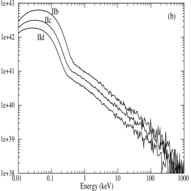
Figure 4.9: The final emitted spectra for different disk rates are shown for (a) $\lambda=1.80$ and (b) $1.75$. Corresponding Cases are marked on each curve. The spectrum appears to become softer with the increase in $\dot{m_{d}}$ (see also, GGC12).

In Figs 4.9(a) and (b), we show three spectra for each of the specific angular momentum: (a) $\lambda=1.80$ and (b) $\lambda=1.75$. The Cases are marked. We see that a spectrum is essentially made up of the soft bump (injected multi-colour blackbody spectrum from the Keplerian disk which are unscattered), and a Comptonized spectrum with an exponential cutoff – the cutoff energy being dictated by the electron cloud temperature. As the disk rates are very small ($\sim$ 0.0001 Eddington rate), the temperature of the disk is small and the resulting spectra show peaks at extremely low energies in the above Figure. If we define the energy spectral index $\alpha$ to be $I(E)\propto E^{-\alpha}$ in the region $2-20$ keV, we note that $\alpha$ increases, i.e., the spectrum softens with the increase in $\dot{m}_{d}$. This is consistent with the predictions made by the static models of CT95 and Chakrabarti (1997).

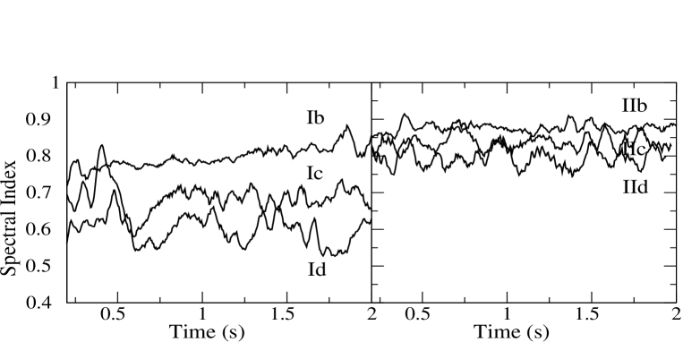
Figure 4.10: Time variation of the spectral index [$\alpha$, $I(E)\propto E^{-\alpha}$] for different disk rates. Different Cases are marked. We note that as the accretion rate goes up, the average $\alpha$ increases, i.e., the spectrum softens (see also, GGC12).

In reality, since the disk is not stationary, the spectrum also varies with time, and so is $\alpha$. In Fig. 4.10, we present the time variation of the spectral index for the different Cases. We clearly see that the spectral index goes up with the increase in the disk accretion rate (see also, GGC12). Thus, on an average, the spectrum softens.

In the above works, we have not considered the effects of magnetic field. In presence of magnetic field, synchrotron photons may be emitted from the post-shock region which affect the spectral shape (Mandal & Chakrabarti 2005a, 2005b; Chakrabarti & Mandal 2006; Mandal & Chakrabarti 2008). Synchrotron emission may occur from the Maxwell-Boltzmann electrons of the pre-shock as well as the CENBOL and jet regions and from the shock accelerated power-law electrons. These photons may get inverse-Comptonized in the CENBOL and produce high energy X and gamma rays extending upto a few MeV, as shown in the above references. These effects are not included in our radiative-hydro calculation.

Chapter 4 QUASI PERIODIC OSCILLATIONS IN A RADIATIVE TRANSONIC FLOW

Quasi-periodic oscillations (QPOs) of observed X-rays are very important features for the study of accreting stellar mass black holes. Observations of QPOs in black hole candidates have been reported quite extensively in the literature (e.g., Remillard & McClintock 2006; Chakrabarti et al. 2008 and the references therein). They are believed to be the manifestations of some regular movements of the underlying accretion flows and happen to be closely connected to the spectral states (Remillard & McClintock 2006; Titarchuk, Shaposhnikov & Arefiev 2007). X-ray transient sources in our galaxy exhibit various types of QPOs with frequencies ranging from $~{}0.001-0.01$ Hz to a few hundreds of Hz. (Morgan, Remillard & Greiner 1997; Paul et al. 1998; Yadav et al. 1999; Remillard & McClintock 2006). However, the quasi-periodic behavior is not always observed. More common feature is the erratic variation of photon count rates even in a timescale of seconds (GGC13).

It has also been reported that there should exist a correlation between the QPO frequency and the spectral index (Remillard & McClintock 2006; Chakrabarti, Debnath, Nandi & Pal 2008; Chakrabarti, Dutta & Pal 2009; Debnath, Chakrabarti & Nandi 2010; Stiele, Belloni, Kalemci & Motta 2013). These authors reported a rise in photon index with increasing centroid frequency of QPOs for various black hole candidates during the rising phase of the outbursts. It is also reported that during the decay phase of the outburst, the trend is time reversed, i.e., a fall in photon index with the decrease of the QPO frequency. The correlation does not depend much on any individual outburst, rather they follow a general trend.

The TCAF model (CT95) which explains the spectral properties quite satisfactorily, has been applied to explain the QPOs. In this model, QPOs are the result of the oscillation of the centrifugal pressure supported shocks. Judging from the rapidity in which the spectral properties change, a realistic model would be where the ‘corona’ itself moves at a shorter timescale. According to the TCAF model, the CENBOL (i.e., the post-shock region) which forms primarily because of the centrifugal barrier in the sub-Keplerian flow, intercepts some of the soft photons emerging from the Keplerian disk and redistributes them in the higher energy bands. In this model, the oscillation of X-ray intensity is caused by the the oscillation of the CENBOL region (MSC96; RCM97; CM00; CAM04) which reprocesses different amounts of soft photons at different phases of oscillation. The numerical simulation of low-angular momentum accretion flows including the thermal cooling (MSC96; CAM04) or dynamical cooling (through outflows, e.g., RCM97) shows clearly that the shocks oscillate with frequencies similar to the observed QPO frequencies.

So far, while the shock-oscillation was generally proposed to be the cause of low frequency QPOs, and the numerical simulations generally showed that this could very well be the case (MSC96; CAM04), there was no attempt to include the Keplerian disk into the simulation and only enhanced power-law cooling was used as a proxy to inverse-Comptonization. In the work presented in this Chapter, we use the time dependent radiation hydrodynamic simulation code which includes both the source of seed photons and actual computation of the production of hard photons through the Comptonization process (GGC13). We analyze the resulting light curves to find the QPOs and other timing properties using the NASA HEAsoft package, as though our output corresponds to observed photon flux. We clearly find a correlation between the flow parameters and the QPO frequencies (GGC13). We vary the accretion rates and study the dependence.

5.1 Simulation set up and procedure

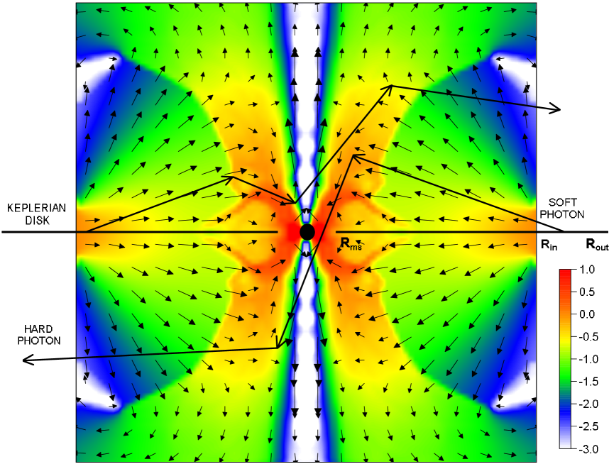
Figure 5.1: The schematic diagram of our simulation set up. The velocity vectors of the infalling matter are shown. The colors show the normalized density in a logarithmic scale. The zig-zag trajectories are the typical paths followed by the photons. Velocity vectors are drawn for $\lambda=1.73$ (GGC13).

In Fig. 5.1, we present a schematic diagram of our simulation set up (GGC13). The simulation set up is similar to the one used in Chapter 4. We consider a TCAF where the standard Keplerian disk is flanked by the sub-Keplerian flow (CT95). The soft photons, emerging out of the Keplerian disk, are intercepted and reprocessed via Compton or inverse-Compton scattering by the sub-Keplerian matter, both in the post-shock and the pre-shock regions. The sub-Keplerian matter enters the simulation box through the outer boundary at $R_{in}$. The outer edge of the Keplerian disk is assumed to be at $R_{out}$ and it extends inside up to the marginally stable orbit $R_{ms}$. A black hole of mass $M_{bh}$ is located at the center.

1 Sub-Keplerian and Keplerian flows

The sub-Keplerian flow is simulated in two dimensions using the TVD code as is done in Chapters 3 and 4. To model the initial injection of matter, we consider an axisymmetric flow of gas in the pseudo-Newtonian gravitational field (PW80) of a non-rotating black hole of mass $M_{bh}=10M_{\odot}$, located at the center in the cylindrical coordinate system $[R,\theta,z]$. Our computational box occupies one quadrant of the $R-z$ plane with $0\leq R\leq 100$ and $0\leq z\leq 100$. All the calculations were performed with $512\times 512$ equi-spaced cells (GGC12; GGC13). Thus, each grid has a size of $0.19$ in units of the Schwarzschild radius ($r_{g}=2GM_{bh}/c^{2}$). The incoming gas enters the box through the outer boundary, located at $R_{in}=100r_{g}$. We have chosen the normalized density of the incoming gas ${\rho}_{in}=1$ for convenience. We provide sound speed $a$ (i.e., temperature) and velocity $v$ of the incoming gas at outer boundary points. Values of $a$ and $v$ are computed in such a way that total specific energy at outer boundary points remains the same as that of the injected energy. In order to mimic the horizon of the black hole at $r_{g}$, we place an absorbing inner boundary at $r=1.5r_{g}$, inside which all material is completely absorbed into the black hole. For the sake of concreteness, we consider the sub-Keplerian flow with a specific angular momentum $\lambda=1.73$ and specific energy $\epsilon=0.0021$. These parameters are chosen so that we find a stable shock solution (Chakrabarti & Das 2001).

The Keplerian disk is the standard Shakura-Sunyaev (SS73) disk. The soft photons are produced from both the surfaces of the Keplerian disk (GGCL10; GGGC11; GGC12). The inner edge of the disk has been kept fixed at the marginally stable orbit $R_{ms}=3r_{g}$, while the outer edge is assumed to be at $R_{out}=200r_{g}$. The source of the soft photon has a multicolor blackbody spectrum and the emission is blackbody type with the local surface temperature $T(R)$ and the disk between radius $R$ to $R+\delta R$ produces $dN(R)$ number of soft photons. The form of $T(R)$ and $dN(R)$ are given in Eq. (1) and (2-7), respectively.

2 Simulation Procedure

All the simulations have been performed using the time dependent radiation hydrodynamic simulation code described in Chapter 3 and 4. The simulation procedure for these cases are similar to the procedure used for the simulations described in Chapter 4 and in GGGC11 and GGC12.

For a particular simulation, we use the Keplerian disk rate ($\dot{m}_{d}$) and the sub-Keplerian halo rate ($\dot{m}_{h}$) as parameters. The specific energy ($\epsilon$) and the specific angular momentum ($\lambda$) determine the hydrodynamic (shock location, number density and velocity variations etc.) and the thermal properties of the sub-Keplerian matter. In the next Section, we present the results and discuss the possible implications (GGC13).

5.2 Results and discussions

Table 5: Parameters used for the simulations and a summary of results (GGC13).
Case ID	$\epsilon,\lambda$	$\dot{m}_{d}$	$\dot{m}_{h}$	${\rm<R_{sh}>}$	$\nu_{QPO}$	$<\alpha>$	$t_{in}\over t_{cool}$
C1	0.0021, 1.73	1e-4	0.1	25.75	No QPO	0.826	0.694
C2	0.0021, 1.73	2e-4	0.1	22.82	10.63	0.853	0.844
C3	0.0021, 1.73	3e-4	0.1	20.39	12.34	0.868	0.954
C4	0.0021, 1.73	4e-4	0.1	18.62	14.63	0.873	0.944
C5	0.0021, 1.73	5e-4	0.1	18.33	22.74	0.901	1.071
C6	0.0021, 1.73	1e-3	0.1	15.02	18.2	1.074	0.993
C7	0.0021, 1.73	1e-2	0.1	3.4	No QPO	1.139	3.558
C8	0.0021, 1.73	1e-1	0.1	3.6	No QPO	1.102	33.236
C9	0.0021, 1.73	3e-4	0.05	23.53	10.74	0.998	0.859
C10	0.0021, 1.73	3e-4	0.15	18.37	22.80	0.797	1.031
C11	0.0021, 1.73	3e-4	0.2	16.78	No QPO	0.757	1.049

In Table 5, we show the parameters used for the simulations and a summary of the results (GGC13). In Column 2, we list the specific energy ($\epsilon$) and the specific angular momentum ($\lambda$) of the sub-Keplerian flow at the outer boundary. Columns 3 and 4 show the Keplerian disk rate ($\dot{m}_{d}$) and sub-Keplerian halo rate ($\dot{m}_{h}$), respectively. Both are in units of Eddington rate. In Column 5, we present the time averaged shock location in $r_{g}$ near the equatorial plane. For some combinations of $\dot{m}_{d}$ and $\dot{m}_{h}$, we find QPOs, about which we shall comment later. In Column 6, we list the QPO frequencies in Hz. The time averaged spectral slope [$\alpha,~{}I(E)\propto E^{-\alpha}$] is given in Column 7. In the last Column, we show the ratio of the infall time scale ($t_{in}$) and the cooling time scale ($t_{cool}$). The case IDs are given in the first Column.

1 Spectral properties

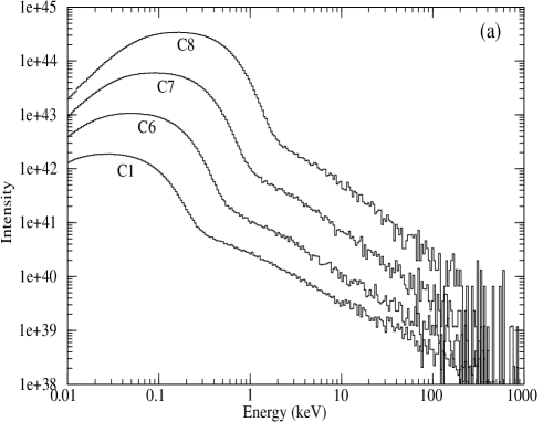
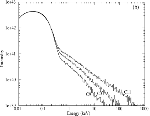
Figure 5.2: a) Variation of the shape of the spectrum when $\dot{m}_{d}$ is increased by a factor of 10 starting from $\dot{m}_{d}=0.0001$ to $0.1$. Case IDs are marked for each plot. The spectrum becomes softer as $\dot{m}_{d}$ is increased. b) Variation of the spectra when the halo rate $\dot{m}_{h}$ is increased keeping the disk rate constant at $\dot{m}_{d}=0.0003$. The spectrum becomes harder as $\dot{m}_{h}$ is increased (GGC13).

In Figs 5.2(a) and (b), we show the variation of the shape of the final emergent spectra (GGC13). In Fig. 5.2(a), the Keplerian disk rate $\dot{m}_{d}$ is increased by a factor of 10 starting from $\dot{m}_{d}=10^{-4}$, keeping the sub-Keplerian halo rate constant at $\dot{m}_{h}=0.1$ Eddington rate. In Fig. 5.2(b), the sub-Keplerian rate $\dot{m}_{h}$ is increased keeping the Keplerian rate constant at $\dot{m}_{d}=3$e-4. The case IDs are marked on each plot. As $\dot{m}_{d}$ is increased, the relative intensity increases. This is understandable since increasing $\dot{m}_{d}$ increases the number of soft photons in a given energy band. At the same time, number of scatterings among the photons and the electrons increases and hence, the centrifugal pressure dominated inner region (including the post-shock region, when present) is cooled faster and the region collapses. Thus the volume of the post-shock region as well as the number of available hot electrons reduce with the increase of $\dot{m}_{d}$ (see, Chapter 4). Since the high energy power-law part of the spectrum is determined by the number of available hot electrons as well as the size of the post-shock region, the spectra become softer with the increase of $\dot{m}_{d}$. On the other hand, the spectra become harder as $\dot{m}_{h}$ is increased. As $\dot{m}_{h}$ is increased, the density of post-shock region increases and hence, the optical depth in this region is enhanced. This increases the number of scatterings and hence, more photons get inverse-Comptonized. Therefore, the number of high energy photons in a given energy band increases. Thus, the spectra become harder (GGC13).

For both the cases (increase in either $\dot{m}_{d}$ or $\dot{m}_{h}$, keeping the other constant), the interaction between the photons and the electrons is enhanced and as a result, the electrons get cooler. Therefore, the shock location moves towards the black hole (see, Table 5), as was shown for thermal bremsstrahlung earlier (MSC96) and analytically by Das & Chakrabarti (2004), Mondal & Chakrabarti (2013) who include both bremsstrahlung and Comptonization.

Figure 5.3: Time variations of the spectral slope of the power-law part of the spectra are shown. Effects of variations of the disk rate $\dot{m}_{d}$ is shown. Case IDs are marked on each panel (GGC13).

Figure 5.4: Same as Fig. 5.3, but the halo rate $\dot{m}_{h}$ is varied keeping $\dot{m}_{d}$ constant (GGC13).

In Figs 5.3 and 5.4, we show the time variation of the spectral slope $\alpha$ [$I(E)\propto E^{-\alpha}$] for all the cases presented in Table 5. The case IDs are marked on each panel. The time averaged values of the spectral slopes are given in Table 5. However, when we plot the time variations, we find an interesting behaviour, namely, the rocking of the spectrum between hard and soft states (GGC13). The spectral slope oscillates around or near the value 1. We find this effect for many cases e.g., C1, C6, C8 and C9. Among these cases, we find low frequency QPOs for C6 and C9 (see below).

2 Timing properties

We compute the time variations of the photon count rates for all the cases in order to generate simulated light curves (GGC13). In the coupled simulation run, a Monte Carlo simulation is run after each hydrodynamic time step. The photons are emitted continuously during this time of hydrodynamical evolution. However, in our two-step process, we process these photons through the Monte Carlo simulation step. In the Monte Carlo simulation, we track each photon and as soon as it leaves the disk, it is saved in an energy bin as well as in a time bin. We divide the energy range $0.01$ keV to $5000$ keV in $300$ logarithmic energy bins. The time resolution is of $5$ ms. After the run is completed, we rebin these photons with a time bin of $0.01$ s to compute the lightcurves. To count the photons in a given energy band, we add up the photon numbers in each energy bins which fall in the required energy band.

Figure 5.5: The light curves in $0.5-100$ keV range are shown. Here, $\dot{m}_{d}$ is increased keeping $\dot{m}_{h}=0.1$ constant (GGC13). See text for the detailed computational procedure of the light curves.

Figure 5.6: Same as Fig. 5.5, but $\dot{m}_{h}$ is increased keeping $\dot{m}_{d}$ constant at $0.0003$ Eddington rate (GGC13).

In Figs 5.5 and 5.6, we plot light curves in the energy band 0.5 keV to 100 keV (for C7 and C8, 2 keV$~{}<~{}E~{}<~{}100$ keV) (GGC13). The photons in this energy range are mostly the inverse-Comptonized photons. The case IDs are marked on each panel. In Fig. 5.5, the Keplerian rate $\dot{m}_{d}$ is increased keeping the sub-Keplerian rate $\dot{m}_{h}$ constant, whereas in Fig. 5.6, $\dot{m}_{h}$ is increased keeping $\dot{m}_{d}$ constant. In both the Figures, we see that the count rate increases with the increase of the variable parameter (e.g., $\dot{m}_{d}$ or $\dot{m}_{h}$). For Fig. 5.5, it is understandable since increasing $\dot{m}_{d}$ increases the number of available soft photons. On the other hand, when we increase $\dot{m}_{h}$, the optical depth of the post-shock region increases and hence, interception of the photons by the electrons increases. Thus the number of Comptonized photons increases and that explains the increase of count rates with $\dot{m}_{h}$ in Fig. 5.6. The variations in the lightcurves are arising because of the variations in the hydrodynamic and thermal properties of the post-shock region.

Figure 5.7: Power Density Spectra (PDS) of the all cases presented in Fig. 5.5. QPO frequency increases with the increase of $\dot{m}_{d}$ (GGC13).

Figure 5.8: Power Density Spectra (PDS) of the all cases presented in Fig. 5.6. QPO frequency increases with the increase of $\dot{m}_{h}$ (GGC13).

In Figs 5.7 and 5.8, we show the Power Density Spectra (PDS) for all the cases (GGC13). The case IDs are marked in each panel. We find low frequency quasi-periodic oscillations (LFQPO) for some cases. The frequencies are listed in Table 5. We find that LFQPO frequencies increase with the increase of both $\dot{m}_{d}$ and $\dot{m}_{h}$. We have seen that the spectra become softer with the increase of $\dot{m}_{d}$ and with the decrease of $\dot{m}_{h}$. Therefore, from Figs 5.3 and 5.7, we find that the LFQPO increases as the object transits from the harder state to the softer states. We find the opposite behavior in Figs 5.4 and 5.8.

It has been argued in the literature (MSC96; CM00; CAM04; Debnath et al. 2010) that the oscillation in the centrifugal barrier dominated post-shock region (CENBOL) is responsible for the LFQPO observed in the black hole candidates. LFQPO arises when the infall time scale of post-shock matter roughly matches with the cooling time scale. For the present simulations, we find the shape of this hot post-shock region to be mostly paraboloid with the base to be oblate spheroid sometimes. Turbulence and backflow of matter are present sometimes in the post-shock region. Therefore, it is not always easy to calculate the exact infall time scale. In our grid based hydrodynamic simulation, we compute the infall time scale in the following way. We take the average of the radial velocity component over 20 vertical grids starting from the equatorial plane at each radius and compute a radial velocity profile near the equatorial plane:

$$v_{avg}(R)\sim\frac{\sum_{iz=1}^{20}v_{R}(R,iz)}{20},$$

where, $v_{R}(R,1)$ represents the radial component of the velocity on the first grid (i.e., on the equatorial plane), $v_{R}(R,2)$ represents the same on the second grid and so on. Then we calculate the infall time scale as (GGC13),

$$t_{in}=\sum_{R=R_{sh}}^{1.5}\frac{dR}{v_{avg}(R)}.$$

The cooling timescale $t_{cool}$ is easy to compute as it includes only the scalar quantities:

$$t_{cool}=\frac{E_{th}}{\dot{E}}.$$

Here, $E_{th}$ is the total thermal energy in the post-shock region and $\dot{E}$ is the cooling rate in the same region, which we calculate directly from the Monte Carlo simulation. In Table 5, we present the ratio $t_{in}\over t_{cool}$ in the last column. We see that this ratio is nearly 1 for all the cases when LFQPOs are seen. Thus the proposal of LFQPOs arising out of resonance oscillation (MSC96; CAM04) of the post-shock region appears to be justified. However, so far, only the power-law cooling was used as the proxy to the Compton cooling. In the present work, actual Comptonization has been used.

In this Chapter, we have presented results on LFQPO of $>$ 10 Hz. However, LFQPO in this range 1-10 Hz can also be simulated using this simulation procedure. As mentioned earlier, LFQPOs are observed when the resonance between the infall and the cooling time scales occurs (MLC94; CAM04) and the frequency of the LFQPO can be found to be $\nu\propto R_{sh}^{-3/2}$, where $R_{sh}$ is the shock location (CM00; Chakrabarti et al. 2008; Debnath et al. 2010; Nandi, Debnath, Mandal, Chakrabarti 2012; Debnath, Chakrabarti, Mondal 2014). Thus, when the shock forms closer, we find LFQPOs on higher side ($\sim$ 10 Hz) and when shock forms far way, LFQPOs of lower side (1-10 Hz or even lower) is found. In the present work, we have done simulations for accretion disk with angular momentum $\lambda=1.73$ for which the shocks from at a radial distance $\sim 20R_{g}$. For higher $\lambda$ with same disk-halo rate parameters, the shock is expected to form at larger radius and we may get 1-10 Hz LFQPOs if the resonance condition is satisfied.

Chapter 5 CONCLUSIONS AND FUTURE PLANS

Here we summarize the main conclusions of the work. This will be followed by the current activities and the future plans.

Summary and conclusions

Here we present the summary of the works that are presented in different Chapters and write down the main conclusions drawn. Most of the findings regarding the spectral and timing properties of a black hole were conjectured (or, even shown) earlier through analytical or numerical methods. These were: State transitions are possible by variations of the disk and halo accretion rates in a TCAF (CT95; Chakrabarti 1997); A direct correlation between the outflow rates and the spectral states must be present (Chakrabarti 1998b; C99; Das et al. 2001); Low Frequency Quasi-Periodic Oscillations (LFQPOs) are the results of oscillation of centrifugal pressure dominated shocks in a transonic flow and the oscillations are due to resonance between the cooling and infall time scales (MSC96; CAM04). In this thesis, by incorporating the effects of radiative cooling (through Monte Carlo method) on the hydrodynamic solutions, we rigorously prove that indeed the spectral and timing properties of a TCAF are exactly as conjectured before.

In Chapter 1, we gave a brief introduction about the theoretical models of the accretion disk around a black hole and described the relevant radiative processes. After that, we discussed about the developments of the numerical techniques to study the dynamics as well as the radiative processes inside an accretion flow.

In Chapter 2, we described our simulation procedure for computing the Comptonized spectrum from a two component advective flow in presence of an outflow. The simulation was carried out using a Monte Carlo code and to reduce the computational time, we parallelized this code. We computed the effects of the thermal and the bulk motion Comptonization on the soft photons emitted from a Keplerian disk by the CENBOL, the pre-shock, sub-Keplerian disk and the outflowing jet (GGCL10). We studied the emerging spectrum when the converging inflow and the diverging outflow (generated from the CENBOL) are simultaneously present. The converging inflow up-scatters the photons and the diverging outflow down-scatters them. The interplay between the up-scattering and down-scattering effects determines the overall shape of the emerging spectrum. The outflow parameters strongly depend on the inflow parameters and hence, for a given inflow and outflow geometry, the strength of the shock can also determine whether the net scattering by the jet would be significant or not. It is also found that sometimes the halo can Comptonize and harden the spectrum by bulk motion Comptonization even without the CENBOL.

In Chapter 3, we described the development of the time dependent radiation hydrodynamic simulation code (GGGC11; GGC12; GGC13). In this code, we coupled the Monte Carlo code with a time dependent hydrodynamic simulation code. The details of the hydrodynamic code and the coupling procedure are given. Using this code, we studied the spectral and timing properties of the Two Component Advective Flows or TCAF. The accreting halo is assumed to be of zero angular momentum and spherically symmetric. It intercepts the soft photons coming out from the Keplerian disk residing on the equatorial plane. We found that in presence of the axisymmetric disk, an originally spherically symmetric accreting Compton cloud could become axisymmetric. This happens because, due to higher optical depth, there is a significant cooling near the axis of the intervening accreting halo between the disk and the axis. We also found the emitted spectrum to be direction dependent. The spectrum along the axis shows a large soft bump, while the spectrum along the equatorial plane is harder. The photons which spend more time (up to 100ms in the case considered) inside the halo are found to produce the harder part of the spectrum as they suffer more scatterings. However, if they spend more than 100ms, they transfer their energy to the relatively cooler electrons before escaping. These results would be important while interpreting the timing properties of the radiations from the black hole candidates. We also explored the effects of the bulk motion of the halo. We found that the inflowing matter push the photons towards inner radius and hence force them to suffer more scatterings resulting in harder spectrum.

In Chapter 4, we studied the effects of the Compton cooling on the outflow in a TCAF using the time dependent radiation hydrodynamic simulation code (GGC12). In this case, the accreting halo is assumed to have some angular momentum with respect to the central black hole and a shock is found to form in the accreting halo. The outflow is found to produce from the CENBOL region. By simulating several cases for different inflow parameters, we showed that the outflow rate is reduced for higher Keplerian disk rate. This happens because the number of injected soft photons increases with increasing disk rate, which cool the electrons of the post-shock region faster. This enhanced cooling reduces the thermal pressure of this region and the post-shock/CENBOL region shrinks. Therefore, the spectrum also becomes softer as the high energy power law part of the spectrum is determined by the number of hot electrons as well as the size of the post-shock region. We, thus, found a direct correlation between the outflow rates and the spectral states of the accreting black holes.

In Chapter 5, we studied the quasi-periodic oscillations in the radiative transonic accretion flows (GGC13). We considered TCAF as the flow configuration and assumed the accreting halo to have some angular momentum. We simulated several cases by varying the disk and the halo rates. The transition from a hard state to a soft state is found to be determined by the mass accretion rates of the disk and the halo. Low frequency QPOs are found for several combinations of disk and halo rates. We found that the QPO frequency increases and the spectrum becomes softer as we increase the Keplerian disk rate. We also found that an earlier prediction that QPOs occur when the infall time scale roughly matches with the cooling time scale, originally obtained using a power-law cooling, remains valid even for Compton cooling. Our findings agree with the general observations of QPOs.

Current activity and future plan

At present, we are working to include the effects of photon bending into our Monte Carlo simulation code. In our simulations, the low energy photons are generated within the accretion disk (from the surface of the Keplerian disk). They travel through the space-time around the black hole before escaping from the accretion disk. The photon trajectory can be calculated by solving the geodesic equations in a given space-time. For the present case, we solve the geodesic equations in the Schwarzschild space-time (Chattopadhyay, Garain & Ghosh 2012). The equations and the solution procedure are described in Appendix A. We are in the process of incorporating the photon transport in Schwarzschild space-time into our simulation. Our approach is the emitter-to-observer approach i.e., the photons are originated inside the accretion disk and are traced till it reaches the observer. This approach is required particularly when the scattering process is included (Schnittman & Krolik 2013).

We also started to include the effects of viscosity in our time dependent radiation hydrodynamic simulation code. Very recently Giri & Chakrabarti (2013) has shown that the Keplerian disk can be formed by incorporating the effects of viscous transport and radiative cooling. A high viscosity in the equatorial plane produces a Keplerian disk while lower viscosity away from the equatorial plane fails to convert the sub-Keplerian flow into a Keplerian disk. Till now, instead of adding viscosity to the flow, we directly included a Keplerian disk as the supplier of the seed photons in the equatorial plane. However, the most self-consistent solution needs to incorporate the viscosity and produce the Keplerian disk, and its spectrum ab initio. This is being investigated into.

Another work we are planning to do in near future is to fit the observed spectrum using our simulation code. For this, we have to simulate several spectra by varying the flow parameters. From the fitting, we shall be able to calculate different flow parameters e.g., the accretion rates of Keplerian and sub-Keplerian flow etc.

Chapter 6 GEODESIC EQUATIONS IN SCHWARZSCHILD SPACE-TIME

The Geodesic equations (Weinberg 1972) in Schwarzschild space-time are the following:

$$\frac{d^{2}r}{dp^{2}}+\frac{A^{\prime}(r)}{2A(r)}\left(\frac{dr}{dp}\right)^{2}-\frac{r}{A(r)}\left(\frac{d\theta}{dp}\right)^{2}-\frac{r\sin^{2}\theta}{A(r)}\left(\frac{d\phi}{dp}\right)^{2}+\frac{B^{\prime}(r)}{2A(r)}\left(\frac{dt}{dp}\right)^{2}=0,\\$$

$$\frac{d^{2}\theta}{dp^{2}}+\frac{2}{r}\frac{d\theta}{dp}\frac{dr}{dp}-\sin\theta\cos\theta\left(\frac{d\phi}{dp}\right)^{2}=0,\\$$ (7-1)

$$\frac{d^{2}\phi}{dp^{2}}+\frac{2}{r}\frac{d\phi}{dp}\frac{dr}{dp}+2\cot\theta\frac{d\phi}{dp}\frac{d\theta}{dp}=0,\\$$

$$\frac{d^{2}t}{dp^{2}}+\frac{B^{\prime}(r)}{B(r)}\frac{dt}{dp}\frac{dr}{dp}=0,$$

where, $A(r)=\left(1-\frac{1}{r}\right)^{-1}$ and $B(r)=\left(1-\frac{1}{r}\right)$.
The last equation of the set of Eq. (7-1) gives

$$\frac{dt}{dp}=\frac{E}{B(r)}=\frac{E}{1-\frac{1}{r}},$$

where, $E$ is a constant of motion (energy-at-infinity) (ST83). Using this equation, we have replaced the derivative w.r.t affine parameter $p$ to $t$ from the above equations to get the following equations:

$$\frac{d^{2}r}{dt^{2}}-\frac{3}{2}\frac{1}{r(r-1)}\left(\frac{dr}{dt}\right)^{2}-(r-1)\left(\frac{d\theta}{dt}\right)^{2}-(r-1)\sin^{2}\theta\left(\frac{d\phi}{dt}\right)^{2}+\frac{r-1}{2r^{3}}=0,\\$$

$$\frac{d^{2}\theta}{dt^{2}}+\frac{2r-3}{r(r-1)}\frac{dr}{dt}\frac{d\theta}{dt}-\sin\theta\cos\theta\left(\frac{d\phi}{dt}\right)^{2}=0,\mathrm{~{}and~{}}\\$$ (7-2)

$$\frac{d^{2}\phi}{dt^{2}}+\frac{2r-3}{r(r-1)}\frac{dr}{dt}\frac{d\phi}{dt}+2\cot\theta\frac{d\theta}{dt}\frac{d\phi}{dt}=0.$$

The set of Eq. (7-2) is solved using the fourth order Runge Kutta method. To start the integration, we need to know the initial location of the photon ($r,\theta,\phi$) and its initial direction of movement ($v^{\hat{r}},v^{\hat{\theta}},v^{\hat{\phi}}$), where,

$$v^{\hat{r}}={r\over(r-1)}{dr\over dt};\;v^{\hat{\theta}}={r\sqrt{r}\over\sqrt{(r-1)}}{d\theta\over dt};\;v^{\hat{\phi}}={r\sqrt{r}\sin\theta\over\sqrt{(r-1)}}{d\phi\over dt}.$$

In the Monte Carlo simulation, the initial location of a photon and its propagation direction are randomized using the given distribution functions. With these initial values, the photon path is computed by solving the above equations till it suffers a scattering or leaves the electron cloud. In case the photon get scattered by an electron, it is tracked subsequently from the scattering location with the new direction of propagation.

References

- Abramowicz M., Czerny B., Lasota J. P., Szuszkiewicz E., 1988, ApJ, 332, 646
- Appl S., Camenzind M., 1993, A&A, 270, 71
- Blandford R. D., Begelman M. C., 1999, MNRAS, 303, L1
- Blandford R. D., Eichler D., 1987, Physics Report, 174, 2
- Blandford R. D., Payne D. G., 1982, MNRAS, 199, 883
- Blandford R. D., Rees M. J., 1974, MNRAS, 169, 395
- Bradt H. V. D., McClintock J. E., 1983, Ann. Rev. of Astron. Astrophys., 21, 13
- Bondi H., 1952, MNRAS, 112, 195
- Cambier H. J., Smith D., 2013, ApJ, 767, 46
- Chakrabarti S. K., 1986, ApJ, 303, 582
- Chakrabarti S. K., 1989a, ApJ, 337, L89
- Chakrabarti S. K., 1989b, ApJ, 347, 365
- Chakrabarti S. K., 1990, Theory of Transonic Astrophysical Flows, World Scientific, Singapore (C90)
- Chakrabarti S. K., 1996, Physics Report, 266, 229 (C96)
- Chakrabarti S. K., 1996, MNRAS, 283, 325
- Chakrabarti S. K., 1996, ApJ, 471, 237
- Chakrabarti S. K., 1997, ApJ, 484, 313
- Chakrabarti S. K., 1998a, in Observational Evidence for the Black Holes in the Universe, p. 19 (astro-ph/9807104)
- Chakrabarti S. K., 1998b, Ind. Jour. of Phys., 72B, 565 (astro-ph/9810412)
- Chakrabarti S. K., 1998c, arXiv:astro-ph/9801079
- Chakrabarti S. K., 1999, A&A, 351, 185 (C99)
- Chakrabarti S. K., 2004, in Frontiers in Astrophysics, Eds S.K. Chakrabarti, p. 14 (astro-ph/0402562)
- Chakrabarti S. K., 2005, Astrophysics and Space Science, 297, 131
- Chakrabarti S. K., 2010, in AIP Conf. Proc. of 4th Gamow Int. Conf. on Astrophys. & Cosm. After Gamow, 1206, 244
- Chakrabarti S. K., Acharyya K., Molteni D., 2004, A&A, 421, 1 (CAM04)
- Chakrabarti S. K., Das S., 2001, MNRAS, 327, 808
- Chakrabarti S. K., Debnath D., Pal P. S., Nandi A., Sarkar R., Samanta M. M., Wiita P. J., Ghosh H., Som D., 2008, in Proc. 11th Marcel Grossman Meeting on General Relativity, Eds. H. Kleinert, R. T. Jantzen & R. Ruffini, World Scientific, 569
- Chakrabarti S. K., Debnath D., Nandi A., Pal P. S., 2008, A&A, 489, L41
- Chakrabarti S. K., Dutta B. G., Pal P. S., 2009, MNRAS, 394, 1463
- Chakrabarti S. K., Manickam S. G., 2000, ApJ, 53, L41 (CM00)
- Chakrabarti S. K., Mandal S., 2006, ApJ, 642, L49
- Chakrabarti S. K., Mondal S., 2006, MNRAS, 369,976
- Chakrabarti S. K., Molteni D., 1993, ApJ, 417, 671
- Chakrabarti S. K., Molteni D., 1995, MNRAS, 272, 80
- Chakrabarti S. K., Titarchuk L. G., 1995, ApJ, 455, 623 (CT95)
- Chattopadhyay I., Das S., Chakrabarti S. K., 2004, MNRAS, 348, 846
- Chattopadhyay I., Garain S. K., Ghosh H., submitted, Proc. of International Conference on Astrophysics and Cosmology (2012), Tribhuvan University, Nepal
- Colbert E. J. M., Mushotzky R. F., 1999, ApJ, 519, 89
- Das S., Chattopadhyay I., Nandi A., Chakrabarti S. K., 2001, A&A, 379, 683
- Das S., Chakrabarti S. K., 2004, Int. J. Mod. Phys. D, 13, 1955
- Das S., Chattopadhyay I., 2008, New Astron., 13, 549
- Debnath D., Chakrabarti S. K., Mondal S., 2014, arXiv:astro-ph/1402.0989
- Debnath D., Chakrabarti S. K., Nandi A., 2010, A&A, 520, 98
- Dewangan G. C., Titarchuk L., Griffiths R. E., 2006, ApJ, 637, L21
- Dutta B. G., Chakrabarti S. K., 2010, MNRAS, 404, 2136
- Eardley D. K., Lightman A. P., Shapiro S. L., 1975, ApJ, 199, L153
- Eggum G. E., Coroniti F. V., Katz J. I., 1987, ApJ, 323, 634
- Eggum G. E., Coroniti F. V., Katz J. I., 1988, ApJ, 330, 142
- Fender R. P., Belloni T. M., Gallo E., 2004, MNRAS, 355, 1105
- Fender R. P., Gallo E., Russell D., 2010, MNRAS, 406, 1425
- Frank J., King A., Raine D. J., 2002, Accretion Power in Astrophysics (Cambridge University Press, UK) (FKR)
- Fukue J., 1983, PASJ, 35, 539
- Gallo E., Fender R. P., Pooley G., 2004, NuPhS, 132, 363
- Garain S. K., Ghosh H., Chakrabarti S. K., 2012, ApJ, 758, 114 (GGC12)
- Garain S. K., Ghosh H., Chakrabarti S. K., to appear, MNRAS (2013) (GGC13)
- Ghosh H., Chakrabarti S. K., Laurent P., 2009, Int. J. Mod. Phys. D, 18, 1693
- Ghosh H., Garain S. K., Chakrabarti S. K., Laurent P., 2010, Int. J. Mod. Phys. D, 19, 607 (GGCL10)
- Ghosh H., Garain S. K., Giri K., Chakrabarti S. K., 2011, MNRAS, 416, 959 (GGGC11)
- Gingold R. A., Monaghan J. J., 1977, MNRAS, 181, 375
- Giri K., Chakrabarti S. K., Samanta M. M., Ryu D., 2010, MNRAS, 403, 516
- Giri K., Chakrabarti S. K., 2012, MNRAS, 421, 666
- Giri K., Chakrabarti S. K., 2013, MNRAS, 430, 2836
- Harten A., 1983, Jour. of Comp. Phys., 49, 357
- Hawley J., Smarr L., Wilson J., 1984a, ApJ, 277, 296
- Hawley J., Smarr L., Wilson J., 1984b, ApJSS, 55, 211
- Hawley J. F., Smarr L. L., 1986, in AIP Conf. Proc. Vol. 144, Magnetospheric Phenomena in Astrophysics, ed. R. Epstein & W. Feldman (Melville, NY: AIP), p. 263
- Hua X., Titarchuk L., 1995, ApJ, 449, 188
- Junor W., Biretta J. A., Livio M., 1999, Nature, 401, 891
- Katz J. I., 1976, ApJ, 206, 910
- Kompaneets A. S., 1956, Zh. Eksp. Teor. Fiz., 31, 876 [English transl. Soviet Phys. - JEPT, 4, 730 (1957)]
- Landau L. D., Lifshitz E. M., 1987, Fluid Mechanics (Pergamon Press: Oxford)
- Lanzafame G., Molteni D., Chakrabarti S. K., 1998, MNRAS, 299, 799
- Laurent P., Titarchuk L., 1999, ApJ, 511, 289
- Laurent P., Titarchuk L., 2001, ApJ, 562, L67
- Laurent P., Titarchuk L., 2007, ApJ, 656, 1056
- Longair M. S., 2011, High Energy Astrophysics (Cambridge University Press: New York)
- Lucy L., 1977, AJ, 82, 1013
- Lynden-Bell D., 1969, Nature, 223, 690
- Malkan M. M., Sargent W. L. W., 1982, ApJ, 254, 22
- Malkan M. M., 1983, ApJ, 268, 582
- Mandal S., Chakrabarti S. K., 2005a, A&A, 434, 839
- Mandal S., Chakrabarti S. K., 2005b, Ap&SS, 297, 169
- Mandal S., Chakrabarti S. K., 2008, ApJ, 689, L17
- McClintock J. E., Narayan R., Steiner J. F., 2013, arXiv:astro-ph/1303.1583v2
- Monaghan J. J., 1983, Comput. Phys. Rep., 3, 71
- Monaghan J. J., 1992, ARA&A, 30. 543
- Mondal S., Chakrabarti S. K., 2006, MNRAS, 371, 1418
- Mondal S., Chakrabarti S. K., 2013, MNRAS, 431, 2716
- Molteni D., Lanzafame G., Chakrabarti S. K., 1994, ApJ, 425, 161 (MLC94)
- Molteni D., Ryu D., Chakrabarti S. K., 1996, ApJ, 470, 460 (MRC96)
- Molteni D., Sponholz H., Chakrabarti S. K., 1996, ApJ, 457, 805 (MSC96)
- Morgan E. H., Remillard R. A., Greiner J., 1997, ApJ 482, 993
- Nandi A., Debnath D., Mandal S., Chakrabarti S. K, 2012, A&A, 542, 11
- Nandi A., Manickam S. G., Rao A. R., Chakrabarti S. K., 2001, MNRAS, 324, 267
- Narayan R., Yi I., 1994, ApJ, 428, L13
- Narayan R., Yi I., 1995, ApJ, 444, 231
- Novikov I. D., Thorne K. S., 1973, Black holes (Les astres occlus), p. 343
- Pacheco P. S., Ming W. C., 1997, MPI Users’ Guide in FORTRAN
- Paczyński B., Wiita P. J., 1980, A&A, 88, 23 (PW80)
- Patruno A., Zwart S. P., Dewi J., Hopman C., 2006, MNRAS, 370, L6
- Paul B., Agrawal P. C., Rao A. R., Vahia M. N., Yadav J. S., 1998, ApJ, 492, L63
- Poznyakov L., Sobol I., Sunyaev R., 1976, Soviet Astronomy Letters, 2, 55 (Translation)
- Poznyakov L., Sobol I., Sunyaev R., 1977, Soviet Astronomy, 21, 708 (Translation)
- Poznyakov L., Sobol I., Sunyaev R., 1983, A & Sp Physics Reviews, 2, 189 (PSS83)
- Pringle J. P., Rees M. J., 1972, A&A, 21, 1
- Proga D., 2007, ApJ, 661, 693
- Proga D., Ostriker J. P., Kurosawa R., 2008, ApJ, 676, 101
- Rao A. R., Naik S., Vadawale S. V., Chakrabarti S. K., 2000, A&A, 360, L25
- Rees M. J., 1984, Ann. Rev. Astron. Astrophys., 22, 471
- Rees M., Begelman M., Blandford R., Phinney E., 1982, Nature, 295, 17
- Remillard R. A., McClintock J. E., 2006, Ann. Rev. of Astron. Astrophys., 44, 49
- Rybicki G., Lightman A. P., 1979, Radiative Processes in Astrophysics (New York: Wiley Interscience) (RL79)
- Ryu D., Ostriker J. P., Kang H., Cen R., 1993, ApJ, 414, 1
- Ryu D., Brown G. L., Ostriker J. P., Loeb A., 1995, ApJ, 452, 364
- Ryu D., Chakrabarti S. K., Molteni D., 1997, ApJ, 474, 378 (RCM97)
- Schnittman J. D., Krolik J. H., 2013, arXiv:astro-ph/1302.3214v2
- Smith D., Heindl W., Swank J., 2002, ApJ, 569, 362
- Shapiro S. L., Teukolsky S. A., 1983, Black Holes, White Dwarfs and Neutron Stars (John Wiley & Sons, New York) (ST83)
- Shakura N. I., 1972, Astron. Zh., 49, 921
- Shakura N. I., Sunyaev R. A., 1973, A&A, 24, 337 (SS73)
- Sobol I. M., 1994, A Primer to the Monte Calro Method, CRC Press, US
- Stiele H., Belloni T. M., Kalemci E., Motta S., 2013, MNRAS, 429, 2655
- Sun W., Malkan M. M., 1989, ApJ, 364, 68
- Sunyaev R., Trumper J., 1979, Nature, 279, 506
- Sunyaev R. A., Titarchuk L. G., 1980, A&A, 86, 121
- Sunyaev R. A., Titarchuk L. G., 1985, A&A, 143, 374
- Thorne K. S., Price R. H., 1975, ApJ, 195, L101
- Titarchuk L., 1994, ApJ, 434, 570
- Titarchuk L., Lyubarskij Y., 1995, ApJ, 450, 876
- Titarchuk L., Shaposhnikov N., Arefiev V., 2007, ApJ, 660, 556
- Ueda Y., Yamaoka K., Sánchez-Fernández C., Dhawan V. et al., 2002, ApJ, 571, 918
- Weinberg S., 1972, Gravitation and Cosmology (John Willey & Sons, UK)
- Wichmann B. A., Hill I. D., 1982, Applied Statistics, 31, 188
- Wilson J. R., 1972, ApJ, 173, 431
- Yadav J. S., Rao A. R., Agrawal P. C., Paul B., Seetha S., Kasturirangan K., 1999, ApJ, 517, 935