Many-faced cells and many-edged faces
in 3D Poisson-Voronoi tessellations

Abstract

Motivated by recent new Monte Carlo data we investigate a heuristic asymptotic theory that applies to $n$-faced 3D Poisson-Voronoi cells in the limit of large $n$. We show how this theory may be extended to $n$-edged cell faces. It predicts the leading order large-$n$ behavior of the average volume and surface area of the $n$-faced cell, and of the average area and perimeter of the $n$-edged face. Such a face is shown to be surrounded by a toroidal region of volume $n/\lambda$ (with $\lambda$ the seed density) that is void of seeds. Two neighboring cells sharing an $n$-edged face are found to have their seeds at a typical distance that scales as $n^{-1/6}$ and whose probability law we determine. We present a new data set of $4\times 10^{9}$ Monte Carlo generated 3D Poisson-Voronoi cells, larger than any before. Full compatibility is found between the Monte Carlo data and the theory. Deviations from the asymptotic predictions are explained in terms of subleading corrections whose powers in $n$ we estimate from the data.

Keywords: Three-dimensional Poisson-Voronoi diagram, many-faced cells, many-sided faces, Monte Carlo, statistical theory

LPT-Orsay-14-34

1 Introduction

S patial tessellations are of interest because of their wide applicability. The perhaps simplest model of a disordered cellular structure is the Poisson-Voronoi tessellation obtained by constructing Voronoi cells around point-like ‘seeds’ distributed randomly and uniformly in space. Whereas two- and three-dimensional Poisson-Voronoi cells are relevant for real-life cellular structures, the higher-dimensional case has applications in data analyses of various kinds. An excellent overview of the many applications is given in the monograph by Okabe et al. [1].

Beginning with the early work of Meijering [2], much theoretical effort has been spent on finding exact analytic expressions for the basic statistical properties of the Voronoi tessellation, in particular in spatial dimensions $d=2$ and $d=3$. Quantities of primary interest are the probability $p_{n}(d)$ that a cell have exactly $n$ sides (in dimension $d=2$) or $n$ faces (in dimension $d=3$). Among the very few analytic results that are available for these quantities, there is a determination [3, 4] of the asymptotic behavior of $p_{n}(2)$ in the large-$n$ limit. That calculation also yields the asymptotic behavior of the average area and perimeter of the two dimensional $n$-sided cell. Following that exact work a heuristic theory was developed [5], valid again in the large-$n$ limit, that for $d=2$ reproduces the exact results and that may also be applied in dimension $d>2$. In this work we will confront the predictions of this ‘large-$n$ theory’, as we will call it, with newly obtained Monte Carlo data on 3D Poisson-Voronoi cells.

Large-$n$ theory is based on the idea that certain properties of a large $n$ cell, just like those of a statistical system in the thermodynamic limit, acquire sharply peaked probability distributions that may for many purposes be replaced with their averages. We will be interested in the most characteristic cell properties, viz. the average volume $V_{n_{F}}$ and surface area $S_{n_{F}}$ of an ${n_{F}}$-faced cell, and the average area $A_{n_{E}}$ and perimeter $P_{n_{E}}$ of an ${n_{E}}$-edged cell face. Large-$n$ theory assumes that for ${n_{F}}\to\infty$ the ${n_{F}}$-faced cell tends to a sphere and predicts the leading asymptotic behavior of $V_{n_{F}}$ and $S_{n_{F}}$, viz. power laws in ${n_{F}}$, including their prefactor. We here extend this theory such as to also make predictions for $A_{n_{E}}$ and $P_{n_{E}}$ as ${n_{E}}\to\infty$.

It appears that in the case of the many-edged face an important role is played by the distance, to be called $2L$, between the seeds of the cells sharing that cell face. We will refer to $L$ as the ‘focal distance’ because of a superficial resemblance to the foci of, e.g., an ellipse. The extended theory provides an expression for the probability distribution of $L$ given ${n_{E}}$. It appears that whereas ${A}_{n_{E}}$ and ${P}_{n_{E}}$ increase with ${n_{E}}$, the average focal distance ${L}_{n_{E}}$ decreases  to zero as ${n_{E}}\to\infty$.

Monte Carlo simulation of Poisson-Voronoi cells has a tradition that is many decades old. A computer code developed by Brakke [9] in the 1980’s is still used today. The quality of a Monte Carlo simulation is first of all determined by the number of cells that it has generated.

Recent Monte Carlo work by Mason et al. [6] and by Lazar et al. [7] focused on the statistical topology of networks in two and three dimensions. In Ref. [7] Lazar et al., using Brakke’s code, produced a data set of 250 million three-dimensional Poisson-Voronoi cells, larger than any ever obtained before. The simulation generates successive batches of $10^{6}$ cells from $10^{6}$ seeds randomly and uniformly distributed in a cubic volume with periodic boundary conditions. The authors provided an analysis of their data with strong emphasis on the identification of the frequency of different topological cell types.

In the present work we extend the data set to four billion ($4\times 10^{9}$) three-dimensional cells. We then compare this enlarged data set to large-$n$ theory. We find that in all cases the Monte Carlo data are fully compatible with the predictions of the theory. There appear to be significant large finite size corrections. We discuss to what extent the theoretical law for these subleading terms may be inferred from the data.

This paper is organized as follows. In section 2 we consider first the theory and then the Monte Carlo data for the ${n_{F}}$-faced cell. In section 3 we extend the theory to the ${n_{E}}$-edged cell face and in section 4 we present and discuss the Monte Carlo data for those faces. In section 5 we consider subleading terms to the asymptotic behavior. In section 6 we present a table with our main results and a critical dicussion of their validity. In section 7 we conclude.

2 The many-faced cell

2.1 Theory and simulations

Let there be a three-dimensional Poisson-Voronoi tessellation of seed density $\lambda$. We will take $\lambda=1$ unless stated otherwise. Large-$n$ theory as described in Ref. [5] is directly applicable to the volume and surface area of the three-dimensional ${n_{F}}$-faced cell. We will simply state the results for these quantities and delve deeper into the theory only in section 3. When ${n_{F}}$ gets large, and if we assume that the cell tends towards a sphere of an as yet unknown radius $R_{n_{F}}$, the first neighbor seeds must lie close to a spherical surface of radius $2R_{n_{F}}$. It was shown in Ref. [5] that the volume enclosed by this spherical surface must be such that under unconstrained conditions it would have contained on average ${n_{F}}$ seeds, that is,

$$\frac{4\pi}{3}(2R_{n_{F}})^{3}\simeq{n_{F}}.$$ (2.1)

Throughout, the sign ‘$\simeq$’ will denote an equality valid asymptotically in the limit ${n_{F}}\to\infty$. Eq. (2.1) yields $R_{n_{F}}$ as a function of ${n_{F}}$. The Voronoi cell of the central seed then has a volume ${V}_{n_{F}}$ and surface area ${S}_{n_{F}}$ given by

$$V_{{n_{F}}}^{\rm th}=\frac{4\pi}{3}R_{n_{F}}^{3}\simeq\frac{{n_{F}}}{8},$$ (2.2a)

$$S_{{n_{F}}}^{\rm th}=4\pi R_{n_{F}}^{2}\simeq\left(\frac{9\pi}{16}\right)^{1/3}\!{n_{F}}^{2/3}.$$ (2.2b)

These theoretical averages have been obtained without the aid of any adjustable parameter.

In figure 1 we have presented the Monte Carlo data for $V_{n_{F}}^{\rm MC}$ and $S_{n_{F}}^{\rm MC}$ obtained by averaging over a set of four billion ($4\times 10^{9}$) cells. Each quantity has been divided by its theoretical large-${n_{F}}$ behavior (2.2), so that for both the data points are expected to tend to unity as ${n_{F}}\to\infty$. These data appear to fully conform to this limit behavior, even if the finite-$n$ corrections are still large. We will analyze these subleading terms to the asymptotic laws in section 5.

It is worth noting that Eq. (2.2a) generalizes Lewis’ law [12] for the average area $A^{(2)}_{n}$ of a two-dimensional $n$-sided cell. This law, inspired a long time ago by the study of epithelial cucumber cells, hypothesizes that $A^{(2)}_{n}=cn$ with a coefficient $c$ estimated in the range from 0.20 to 0.25. An exact two-dimensional calculation [4] has shown that this law effectively holds for 2D Poisson-Voronoi cells, albeit only asymptotically, as

$$A^{(2)}_{n}\simeq\frac{n}{4}\,.$$ (2.3)

The two-dimensional large-$n$ theory reproduces the exact result (2.3) and this is one reason why we have confidence that the three-dimensional relations (2.2) are also exact.

2.2 Comments

We conclude this section by a few comments.

1. Balance of entropic forces. Expression (2.1) results [5] from a balance between two ‘forces,’ both of purely entropic origin and extensive in ${n_{F}}$. The first one comes from the necessity – if there is to be an ${n_{F}}$-faced cell – to have ${n_{F}}$ first-neighbor seeds in the vicinity of the central seed; the entropy of such a configuration increases  with the size of the allowable vicinity. The second one comes from the necessity for all other seeds not to interfere, and hence to stay out of an exclusion volume surrounding this vicinity; the entropy of the other seeds decreases  with growing size of the exclusion volume.

2. Local and global deviations from sphericity. The statement that the ‘cell surface tends to a sphere’ may be decomposed into (i) ‘the first-neighbor seeds align along a surface,’ and (ii) ‘this surface tends to a sphere.’ A few words are in place about both.

(i) The local  fluctuations of the first-neighbor positions perpendicular to their surface of alignment is characterized by a width $w_{{n_{F}}}$. The scaling of $w_{n_{F}}$ with ${n_{F}}$ results from the entropy balance; in three dimensions $w_{n}\sim n^{-2/3}$ was found [5].

(ii) How closely the surface of alignment approaches a sphere is determined by its global  properties. It was shown in Ref. [4] that the surface of the two-dimensional $n$-sided cell (actually, a closed curve) is subject to ‘elastic’ deformations at the scale of the cell itself, the elasticity being again of entropic origin. The elastic entropy remains finite as $n\to\infty$ and does not weigh in the entropy balance that determines the two-dimensional $R_{n}^{(2)}$ and $w_{n}^{(2)}$. However, the elastic modes do contribute to the deviations of the surface from sphericity (actually, circularity in 2D).

For finite $n$ there is no sharp distinction between (i) and (ii), but in 2D they were shown to decouple when $n\to\infty$.

3. Monte Carlo evidence for the approach to sphericity. The fluctuations away from sphericity are still fairly large for the values of ${n_{F}}$ that appear in the simulations. Upon assuming a 3D scenario analogous to the one in 2D we conclude that these fluctuations are due to a combination of the nonvanishing shell width $w_{n_{F}}$ and the elastic deformations.

The Monte Carlo results confirm, however, the hypothesized approach to sphericity for the following reason. From Fig. 1 and the known values (2.2) of $V_{n_{F}}^{\rm th}$ and $S_{n_{F}}^{\rm th}$ one sees that the ratio $6\pi^{1/2}V_{n_{F}}^{\rm MC}/(S_{n_{F}}^{\rm MC})^{3/2}$ tends to unity when ${n_{F}}\to\infty$. If $S_{n_{F}}^{\rm MC}$ referred to a single surface enclosing a volume $V_{n_{F}}^{\rm MC}$, this ratio could be unity only if that surface enclosed the largest possible volume, that is, if it were a sphere. For the sharply peaked distribution of surface areas observed in our simulations the same conclusion remains valid.

4. Entropy balance and elastic modes. The nonextensivity of the elastic entropy allows for the entropy balance to be set up without taking into account the elastic modes, that is, by considering the surface of alignment as a sphere right from the start. In the same spirit, when in the next section we will consider seed positions that align along a toroidal surface, we will do so without regard for the elastic deformations of that surface.

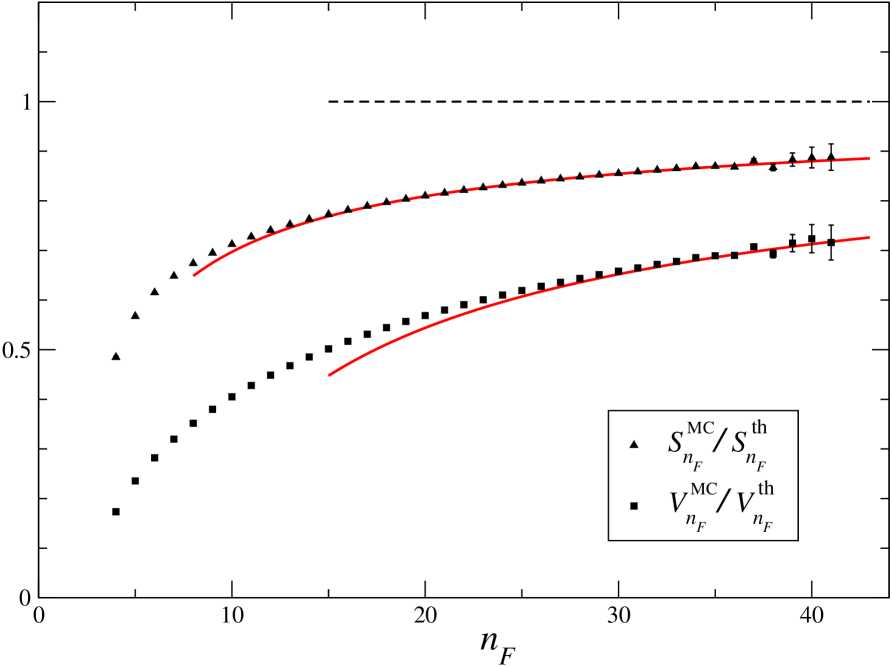
Figure 1: Monte Carlo averages $V_{n_{F}}^{\rm MC}$ and $S_{n_{F}}^{\rm MC}$ of the volume and surface area, respectively, of an ${n_{F}}$-sided cell, each divided by its theoretical asymptotic behavior, Eqs. (2.2). Both sets of data points are predicted, therefore, to tend to unity as ${n_{F}}\to\infty$. The solid red lines approach this limit value as $\sim n^{-2/3}$ and represent our best estimates for the next-order correction to the leading asymptotic behavior (section 5).

3 The many-edged face: theory

3.1 Torus

3.1.1 Preliminaries

Let us consider an arbitrarily selected ${n_{E}}$-edged cell face between two neighboring Voronoi cells. Let the seeds of the two cells (the ‘focal’ seeds) have positions $\mathbf{S}_{1}$ and $\mathbf{S}_{2}$. By a suitable choice of the origin $\mathbf{O}$ and the direction of the $z$ axis we obtain $\mathbf{S}_{1}=(0,0,L)$ and $\mathbf{S}_{2}=(0,0,-L)$, where $L$ is the ‘focal distance’. It is a random variable whose distribution we do not know a priori. The ${n_{E}}$-edged face is then located in the $xy$ plane; a typical face is shown schematically in figure 2. We number its edges by $m=1,2,\ldots,{n_{E}}$ according to increasing polar angle and let $\ell_{m}$ denote the line that prolongs the $m$th edge. We let furthermore $\mathbf{C}_{m}$ denote the projection of the origin $\mathbf{O}$ onto $\ell_{m}$ and $\mathbf{T}_{1},\ldots,\mathbf{T}_{n}$ the vertices of the ${n_{E}}$-edged face.

The $m$th edge is common to the Voronoi cells of $\mathbf{S}_{1}$, $\mathbf{S}_{2}$, and of a third seed whose position we call $\mathbf{F}_{m}$. We will refer to the $\mathbf{F}_{m}$ as the ‘first neighbors’ of the pair $(\mathbf{S}_{1},\mathbf{S}_{2})$. Figure 3 represents the plane through these three seeds, that we will also refer to as the $m$th ‘first-neighbor’ plane. The three planes that perpendicularly bisect the line segments connecting these three seeds intersect along line $\ell_{m}$. This line is perpendicular to the $m$th first-neighbor plane and intersects it in $\mathbf{C}_{m}$, which is therefore equidistant to the three seeds, as shown by the large circular arc of radius $r_{m}$. As announced at the end of section 2, we are assuming that it is safe in this discussion to neglect the elastic deformations of the torus.

Figure 2: Geometry in the plane (‘$xy$’ plane) of the ${n_{E}}$-edged face shared by two cells having their seeds in $\mathbf{S}_{1}$ and $\mathbf{S}_{2}$. The line segment connecting these seeds is perpendicular to this plane and is bisected by it in $\mathbf{O}$. The $m$th edge of the face connects the vertices $\mathbf{T}_{m}$ and $\mathbf{T}_{m+1}$ and lies on a line $\ell_{m}$. The $\mathbf{C}_{m}$ are the projections of $\mathbf{O}$ onto the $\ell_{m}$.

Figure 3: Geometry in the first-neighbor plane plane passing through the seeds $\mathbf{S}_{1}$, $\mathbf{S}_{2}$, and $\mathbf{F}_{m}$. Point $\mathbf{C}_{m}$ is the center of the circle passing through these three seeds. The cell face studied lies in the plane through O perpendicular to the axis of revolution (the ‘$z$’ axis). Rotating the circular arc shown about this axis produces a spindle torus: its minor radius $r_{m}$ is larger than its major radius $R_{m}$. Each dashed line lies in a plane equidistant to two of the three seeds.

3.1.2 Large-$n$ limit

For the cell face of figures 2 and 3 we now develop the following extension of the large-$n$ theory. To simplify notation we write $n$ instead of ${n_{F}}$. Let us consider the subset of faces with fixed focal distance $L$. It is natural to assume that in the limit of large $n$ the area of the $n$-edged face will grow without limit and that its shape will approach a circle of some as yet unknown radius that we will call ${\sf R}_{n}$. More precisely, all $R_{m}/{\sf R}_{n}$ will tend to unity when $n\to\infty$. According to figure 3 there must then also be an ${\sf r}_{n}$ related to ${\sf R}_{n}$ by

$${\sf r}_{n}^{2}={\sf R}_{n}^{2}+L^{2}$$ (3.1)

and which is such that $r_{m}/{\sf r}_{n}$ will tend to unity when $n\to\infty$. In that limit, as $m$ varies from $1$ to $n$, the large circular arc in figure 3 turns around the axis of revolution and describes a torus whose major and minor radii are ${\sf R}_{n}$ and ${\sf r}_{n}$. Since ${\sf R}_{n}\leq{\sf r}_{n}$, this torus has no hole and is actually a spindle torus. The $\mathbf{F}_{m}$ lie close to the surface of this torus in a thin shell whose width $w_{n}$ vanishes with growing $n$. There can be no seeds inside this torus as this would destroy the $n$-edgedness of the face.

3.2 Probability ${\cal P}_{n}$ of occurrence of an $n$-edged face

Given two adjacent cells that share an $n$-edged face, we now ask for the probability ${\cal P}_{n}$ that the two focal seeds be at distance $2L$ and  that the $n$ first neighbor seeds be located in a toroidal shell with minor radius ${\sf r}$, and therefore with major radius ${\sf R}=({\sf r}^{2}-L^{2})^{1/2}$. It will have advantages to express ${\cal P}_{n}$ as a function of the independent variables ${\sf r}$ and

$$x=\frac{L}{{\sf r}}\,.$$ (3.2)

Since it is proportional to the number of microscopic seed configurations compatible with the constraints $(n,{\sf r},x)$, and because of the analogy with thermodynamics, we will refer to $\,\log{\cal P}_{n}({\sf r},x)\,$ as an ‘entropy’. We will now determine an explicit although approximate expression for this entropy and study its variation with ${\sf r}$ and $x$.

Let us write $V_{0}$ for the volume of the torus with parameters ${\sf r}$ and $L$, $S_{0}$ for its surface area, and

$$V_{1}=w_{n}S_{0}$$ (3.3)

for the volume of the shell of width $w_{n}$ at the surface of the torus. Let $\lambda$ (which may be scaled away) be the three-dimensional seed density. We then have

$${\cal P}_{n}({\sf r},x)\simeq\mbox{cst}\times(x{\sf r})^{2}\,\frac{{\rm e}^{-\lambda V_{1}}(\lambda V_{1})^{n}}{n!}\,{\rm e}^{-\lambda V_{0}},$$ (3.4)

in which, here and henceforth, ‘cst’ stands for a constant that may each time be a different one, and where $(x{\sf r})^{2}=L^{2}$ is the phase space factor associated with two seeds being at distance $2L$, the Poisson distribution ${\rm e}^{-\lambda V_{1}}(\lambda V_{1})^{n}/n!$ is the probability that in a random seed distribution of density $\lambda$ the volume $V_{1}$ contain exactly $n$ seeds, and ${\rm e}^{-\lambda V_{0}}$ is the probability that the volume $V_{0}$ contain no seeds. Equation (3.4) is obviously an approximation: for one thing, it does not take into account the detailed individual positions of the first neighbor seeds in $V_{1}$, but only restricts them to the shell. We will take (3.4) seriously, nevertheless, and see where it leads us.

The expressions, needed in (3.4), for the volume $V_{0}$ and the surface $S_{0}$ of the torus with parameters ${\sf r}$ and $x=L/{\sf r}$ are

$$V_{0}=2\pi^{2}{\sf r}^{3}g(x),$$ (3.5a)

$$S_{0}=4\pi^{2}{\sf r}^{2}f(x),$$ (3.5b)

in which

$$\pi f(x)=x+(\pi-\arcsin x)\sqrt{1-x^{2}},$$ (3.6a)

$$\pi g(x)=\pi f(x)-\tfrac{1}{3}x^{3}.$$ (3.6b)

For later use we note the small-$x$ expansions

$$f(x) = 1-\tfrac{1}{2}x^{2}+\frac{1}{3\pi}x^{3}+{\cal O}(x^{4}),$$

$$g(x) = 1-\tfrac{1}{2}x^{2}+{\cal O}(x^{4}).$$ (3.7)

The shell width $w_{n}$, also needed in (3.3), is a function of ${\sf r}$ and $x$ that we will determine in the next section.

3.3 Shell width $w_{n}$

Our determination of $w_{n}$ will exploit an invariance hidden in this problem. The $m$th edge of the face is a segment of a line $\ell_{m}$ that is perpendicular to the plane of figure 3 and intersects this plane in $\mathbf{C}_{m}$. Along $\ell_{m}$ the three Voronoi cells of $\mathbf{S}_{1}$, $\mathbf{S}_{2}$, and $\mathbf{F}_{m}$, join. The faces separating these cells are located in planes that are also perpendicular to the plane of figure 3 and intersect it along the dashed lines passing through $\mathbf{C}_{m}$. Suppose now that seed $\mathbf{F}_{m}$ moves along the circular arc in figure 3. This will leave the position of $\mathbf{C}_{m}$ invariant; hence it will leave line $\ell_{m}$ invariant; and since the set of lines $\{\ell_{m}\}$ determines the perimeter of the face, it will leave the face invariant. We may therefore rotate all first neighbors $\mathbf{F}_{m}$ to a position with $\theta_{m}=0$, that is, a position in the plane of the face, without changing the face. Having performed this rotation (without introducing a new symbol for the rotated $\mathbf{F}_{m}$) we obtain the situation of figure 4. We are now ready to discuss the width $w_{n}$.

The filled black dots in figure 4 are the positions after rotation of the first neighbors $\mathbf{F}_{m}$. For convenience we have chosen them as the vertices of a regular $n$-gon, supposing that this does not affect the argument below in any essential way. The edges of the $n$-gon have midpoints $\mathbf{M}_{m}$. The $\mathbf{T}_{m}$ are the vertices of the $n$-edged face of interest, which is also a regular $n$-gon. The $M_{m}T_{m}$ are the perpendicular bisectors of the $F_{m}F_{m-1}$, where we write here $AB$ for the line segment connecting the two points $\mathbf{A}$ and $\mathbf{B}$. Suppose now that $\mathbf{F}_{m}$ moves along the line through $\mathbf{F}^{\prime}$ and $\mathbf{F}^{\prime\prime}$ (both points marked by filled red dots). The midpoint $\mathbf{M}_{m}$ then moves along a parallel line with corresponding points $\mathbf{M}^{\prime}$ and $\mathbf{M}^{\prime\prime}$. On the left the midpoint $\mathbf{M}_{m+1}$ executes the mirrored motion (not shown). As a consequence line segment $T_{m}T_{m+1}$ is displaced parallel to itself. When it moves down so far that it passes through $\mathbf{T}^{\prime}$, its neighboring segments disappear; and when it moves up so high that it passes through $\mathbf{T}^{\prime\prime}$, it disappears itself. In both cases the face ceases to be $n$-edged. The limit points $\mathbf{T}^{\prime}$ and $\mathbf{T}^{\prime\prime}$ determine $\mathbf{F}^{\prime}$ and $\mathbf{F}^{\prime\prime}$. We will identify somewhat arbitrarily the shell width $w_{n}$ with the segment length $|F^{\prime}F^{\prime\prime}|$, which we calculate as follows. The angle between $F^{\prime}F_{m-1}$ and $F^{\prime\prime}F_{m-1}$ is identical to the one between $T^{\prime}M^{\prime}$ and $T^{\prime\prime}M^{\prime\prime}$. All these angles become very small as $n$ gets large. Neglecting higher order terms in the angles we have

$$\frac{|F^{\prime}F^{\prime\prime}|}{|F_{m}F_{m-1}|}=\frac{|T^{\prime}T^{\prime\prime}|}{|T_{m}M_{m}|}\,.$$ (3.8)

Upon using that the $\mathbf{F}_{m}$ and $\mathbf{T}_{m}$ are vertices of regular polygons and substituting $|F_{m}F_{m-1}|=2\pi({\sf R}+{\sf r})/n$, $|T^{\prime}T^{\prime\prime}|=3\pi{\sf R}/n$, and $|T_{m}M_{m}|={\sf r}$ we obtain

$$w_{n}({\sf r},L) = \frac{6\pi^{2}{\sf R}({\sf R}+{\sf r})}{n^{2}{\sf r}}$$ (3.9)

$$= \frac{C}{2}(1-x^{2}+\sqrt{1-x^{2}})\frac{{\sf r}}{n^{2}}\,,$$

in which $C=12\pi^{2}$ is a constant that will play no role in what follows. We will write

$$\tilde{f}(x)=\frac{1}{2}(1-x^{2}+\sqrt{1-x^{2}})f(x),$$ (3.10)

so that from relations (3.10), (3.3), and (3.5b) we have

$$V_{1}=\frac{4\pi^{2}C{\sf r}^{3}}{n^{2}}\tilde{f}(x).$$ (3.11)

Equations (3.5a) and (3.11) are the desired expressions for $V_{0}$ and $V_{1}$.

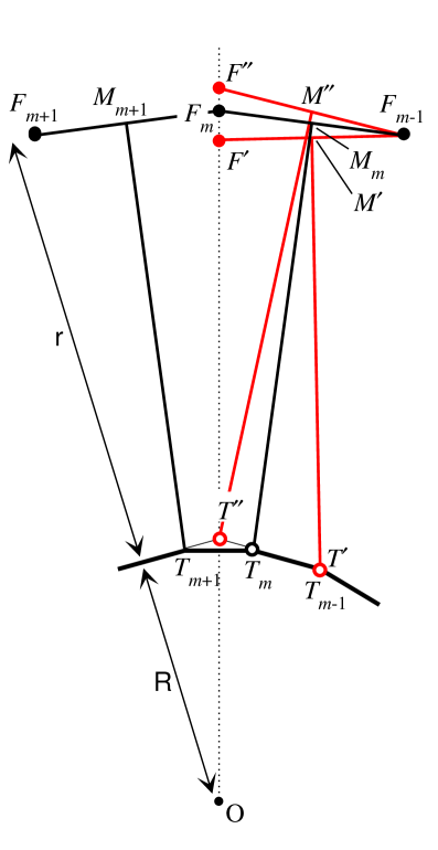
Figure 4: Geometry in the plane of the face after all first neighbor seeds $\mathbf{F}_{j}$ have been rotated as explained in the text. The heavy line linking $\ldots,\mathbf{T}_{m-1},\mathbf{T}_{m},\ldots$ is the face boundary when the $m$th neighbor is located at $\mathbf{F}_{m}$. When $\mathbf{F}_{m}$ moves to $\mathbf{F}^{\prime}$ (or to $\mathbf{F}^{\prime\prime}$), then $\mathbf{T}_{m}$ moves to $\mathbf{T}^{\prime}$ (or to $\mathbf{T}^{\prime\prime}$).

3.4 Analysis of ${\cal P}_{n}({\sf r},x)$

Directly from Eq. (3.4) we have

$$\log{\cal P}_{n}({\sf r},x)\simeq-\lambda V_{1}+n\log\lambda V_{1}-\log n!-\lambda V_{0}+2\log x-\frac{2}{3}\log\lambda{\sf r}^{3},$$ (3.12)

which we will study as a function of its two variables. We may simplify this expression by noting that in the large-$n$ limit $\lambda V_{1}$ is negligible with respect to $\lambda V_{0}$ and $\log\lambda{\sf r}^{3}$ with respect to $n\log\lambda V_{1}$. Some further rewriting is useful. First, we substitute in (3.12) the explicit expressions (3.5a) and (3.11) for $V_{0}$ and $V_{1}$. Second, we may discard from (3.12) any terms that do not depend on ${\sf r}$ or $x$ and that we may recover later by normalizing the distribution. Then, instead of $\log{\cal P}_{n}$ of Eq. (3.12), we may study $\log\bar{{\cal P}}_{n}$ given by

$$\log\bar{{\cal P}}_{n}({\sf r},x)\simeq n\log\Big{(}2\pi^{2}\lambda{\sf r}^{3}\tilde{f}(x)\Big{)}-2\pi^{2}\lambda{\sf r}^{3}g(x)+2\log x.$$ (3.13)

The first two terms represent two opposing entropic forces similar to those referred to in section 2.2 for the case of the ${n_{F}}$-sided cell. We are first of all interested in the variation of $\log\bar{{\cal P}}_{n}$ with ${\sf r}$. For fixed $x$, let (3.13) be maximal for ${\sf r}={\sf r}_{\rm max}(x)$. Setting $\partial\log\bar{{\cal P}}_{n}/\partial(2\pi^{2}\lambda{\sf r}^{3})=0$ we obtain

$$2\pi^{2}\lambda{\sf r}_{\rm max}^{3}(x)g(x)=n.$$ (3.14)

We now note that in view of (3.5a) the first member of the above equation is equal to $\lambda V_{0}$. Eq. (3.14) therefore says that the entropy is maximized when the volume of the torus is such that under unconstrained conditions it would have contained $n$ seeds. This is the torus counterpart of Eq. (2.1).

For $n\to\infty$ the maximum in ${\sf r}$ corresponds to a narrow peak, as may be shown by an expansion of (3.13) about its maximum. The marginal distribution of $x$, defined as the integral of $\bar{{\cal P}}_{n}({\sf r},x)$ with respect to its first argument, is therefore obtained by simply taking ${\sf r}={\sf r}_{\rm max}(x)$ in (3.13), which leads to

$$\bar{{\cal P}}_{n}({\sf r}_{\rm max}(x),x)\simeq\mbox{cst}\times x^{2}\left(\frac{\tilde{f}(x)}{g(x)}\right)^{\!n}.$$ (3.15)

The ratio $\tilde{f}(x)/g(x)$ has its maximum at $x=0$. Upon expanding for small $x$ with the aid of (3.6) and (3.10) we obtain

$$\frac{\tilde{f}(x)}{g(x)}=1-\frac{3}{4}x^{2}+\frac{1}{3\pi}x^{3}+{\cal O}(x^{4}).$$ (3.16)

The term of order $x^{2}$ with the negative coefficient $-3/4$ is the only one that leaves a trace in the limit $n\to\infty$; it stems directly from the factor $(1-x^{2}+\sqrt{1-x^{2}})/2$ in (3.10), which in turn comes from the shell width. Using (3.16) in (3.15) and letting $n\to\infty$ we have to leading order $\bar{{\cal P}}_{n}({\sf r}_{\rm max}(x),x)\to\mbox{cst}\times x^{2}\exp(-(3n/4)x^{2})$, so that $x$ is not sharply peaked but has a well-defined distribution on scale $n^{-1/2}$. More precisely, in that limit the scaled variable

$$y=(3\pi n)^{1/2}x/4$$ (3.17)

has the distribution $Q(y)$ given by

$$Q(y)=32\pi^{-2}y^{2}\exp\left(-\frac{4}{\pi}y^{2}\right),\qquad y>0,$$ (3.18)

where we have restored the normalization, and where $y$ is such that its first moment is unity.

Knowing that $x$ is random on the scale $n^{-1/2}$ we have from (3.2) that $g(x)=1+O(n^{-1})$ and subsequently from (3.14) the small-$x$ expansion

$${\sf r}_{\rm max}(x)={\sf r}_{n}\left[1+{\cal O}(n^{-1})\right]$$ (3.19)

with leading order term

$${\sf r}_{n}=\left(\frac{n}{2\pi^{2}}\right)^{1/3},$$ (3.20)

in which we have set $\lambda=1$. In relation (3.2) we now replace ${\sf r}$ by its leading order value ${\sf r}_{n}$ and obtain, also using (3.20),

$$L \simeq (n/2\pi^{2})^{1/3}x$$ (3.21)

$$= 2^{5/3}3^{-1/2}\pi^{-7/6}n^{-1/6}y.$$

This shows that $L$ varies on scale $n^{-1/6}$. Since $y$ has unit average we now have for the average $L_{n}$ of $L$ the expression

$$L_{n}^{\rm th}\simeq 2^{5/3}3^{-1/2}\pi^{-7/6}n^{-1/6}.$$ (3.22)

Furthermore, as $n\to\infty$ the probability distribution $Q_{n}$ of the scaled variable $y=L/L_{n}^{\rm th}$ is predicted to tend to the fixed law $Q(y)$ of Eq. (3.18). One may loosely rephrase this scaling with $n^{-1/6}$ by saying that the many-edgedness of a cell face leads to an attractive force (of entropic origin) between the two focal seeds. It was not a priori  clear to us that such a phenomenon would occur.

Knowing now that $L$ is distributed on scale $n^{-1/6}$, relation (3.1) tells us that ${\sf r}_{n}$ and ${\sf R}_{n}$ must be equal to leading order, and hence

$${\sf R}_{n}\simeq\left(\frac{n}{2\pi^{2}}\right)^{1/3}.$$ (3.23)

For the shell width $w_{n}$ and the shell volume $V_{1}$ we find with the aid of (3.23), (3.9), (3.3), and (3.5b) the scaling behavior

$$w_{n}\simeq\mbox{cst}\times n^{-5/3},\qquad V_{1}\simeq\mbox{cst}\times n^{-1},$$ (3.24)

where we have preferred to denote the prefactors by ‘cst’ in view of the arbitrariness in the definition of $w_{n}$. Eq. (3.24) tells us that the shell becomes rapidly thinner as $n$ gets larger.

We finally return to the averages $A_{n}$ and $P_{n}$. Having determined that for ${n_{E}}\to\infty$ the ${n_{E}}$-edged cell face tends to a circle of a now known radius ${\sf R}_{n}$ we conclude that

$$A_{n_{E}}^{\rm th}=\pi{\sf R}_{n_{E}}^{2}\simeq(4\pi)^{-1/3}{n_{E}}^{2/3},$$ (3.25a)

$$P_{n_{E}}^{\rm th}=2\pi{\sf R}_{n_{E}}\simeq(4\pi)^{1/3}{n_{E}}^{1/3}.$$ (3.25b)

These relations are analogous to the laws (2.2) for the cell volume and surface area. This completes the extension of large-$n$ theory to the ${n_{E}}$-edged cell face in the limit of asymptotically large ${n_{E}}$.

4 The many-edged face: Monte Carlo

The $4\times 10^{9}$ cells generated by Monte Carlo simulation yielded $N_{n}$ cell faces of edgedness $n$, adding up to a total of $N=\sum_{n}N_{n}=31\,071\,027\,941$ cell faces. The distribution $N_{n}$ has been presented in table 1 together with our estimates of the fractions $f_{n}$ of $n$-edged faces. In Ref. [7] several comparisons with theoretically known data have been presented as a demonstration that the algorithm works correctly. Here we limit ourselves to two such tests, shown in table 2. Let $\langle{n_{F}}\rangle$ and $\langle{n_{E}}\rangle$ stand for the average facedness of a cell and the average edgedness of a cell face, respectively. The rms deviation of ${n_{F}}$ is equal to 3.318, which leads to an estimate of the standard deviation in its Monte Carlo average equal to $3.318/\sqrt{4\times 10^{9}}=0.000\,06$. The rms deviation of ${n_{E}}$ is equal to 1.579, which leads to an estimate of the standard deviation in its Monte Carlo average equal to $1.579/\sqrt{N}=0.000\,009$. The average values from the Monte Carlo simulations together with these standard deviations are shown in the first two lines of table 2. The theoretical values of both averages are exactly known (see e.g. Ref. [1]) and shown in the third line. The agreement between the Monte Carlo values and these exact results is excellent.

$n$	$N_{n}$	$f_{n}$	$n$	$N_{n}$	$f_{n}$
3	4 187 261 126	$0.134\,764\pm 0.000\,002$	12	11 834 735	$(3.809\pm 0.002)\times 10^{-4}\,\,$
4	7 140 019 564	$0.229\,797\pm 0.000\,003$	13	2 174 618	$(6.999\pm 0.005)\times 10^{-5}\,\,$
5	7 505 993 048	$0.241\,575\pm 0.000\,003$	14	342 988	$(1.104\pm 0.002)\times 10^{-5}\,\,$
6	5 914 222 488	$0.190\,345\pm 0.000\,003$	15	46 869	$(1.508\pm 0.007)\times 10^{-6}\,\,$
7	3 621 030 915	$0.116\,540\pm 0.000\,002$	16	5 690	$(1.83\pm 0.03)\times 10^{-7}\,\,$
8	1 747 654 056	$0.056\,247\pm 0.000\,002$	17	613	$(1.97\pm 0.08)\times 10^{-8}\,\,$
9	674 407 674	$0.021\,705\pm 0.000\,001$	18	41	$(1.3\pm 0.2)\times 10^{-9}\,\,$
10	211 374 682	$0.006\,803\pm 0.000\,001$	19	7	$(2.3\pm 0.9)\times 10^{-10}$
11	54 658 826	$0.001\,759\pm 0.000\,001$	20	1	$(3\pm 3)\times 10^{-11}$

Table 1: Observed numbers $N_{n}$ of $n$-edged cell faces in a set of $4\times 10^{9}$ Monte Carlo generated 3D Poisson-Voronoi cells, and their estimated fractions $f_{n}$.

	Expected number $\langle{n_{F}}\rangle$		Expected number $\langle{n_{E}}\rangle$
	of faces of a cell		of edges of a face
Monte Carlo	XXXX15.	535 51	XXXX5.	227 576
Standard deviation	0.	000 06	0.	000 009
Theory	15.	535 457	5.	227 573 4

Table 2: Two tests of the Monte Carlo algorithm.

4.1 Examples of many-edged faces

In the original Monte Carlo simulations by Lazar et al. [7], that comprised $0.25\times 10^{9}$ cells, faces were found with edge numbers up to ${n_{E}}=18$. In figure 5 we show the five $18$-edged faces that occurred, superposed such that their origins coincide. Some faces, such as the red one, are close to circular, but the set shows that there is still considerable variability in shape and size; also, the origin, which for ${n_{E}}\to\infty$ should be at the center of the circle, is still fairly eccentric. It is relevant to recall here that these same observations held for the many-sided two-dimensional cells studied in Ref. [13], for which nevertheless an efficient simulation algorithm has demonstrated the convergence to a circle at higher values of $n$. If the blue face and the gray face seem to have fewer than $18$ edges, this is due to some of their vertices coinciding at the scale of the figure.

Figure 6 is based on the same set of five $18$-edged cell faces. With each face there are associated $18$ planes of the type shown in figure 3, each one passing through the two focal seeds and through one first neighbor seed $\mathbf{F}_{m}$. In figure 6 we have superposed these $5\times 18$ planes such that the points $\mathbf{C}_{m}$ coincide in a single point called $\mathbf{C}$ (this blurs of course the positions of the focal seeds). The positions $(r_{m},\theta_{m})$ with respect to $\mathbf{C}$, defined in figure 3, of the first neighbor seeds $\mathbf{F}_{m}$ are shown. The figure clearly shows the appearance of the hull of a spindle torus, indicated by the circular arc. We have chosen in this figure a radius ${\sf r}_{\rm av}$ as well as somewhat arbitrary values for $L_{\rm av}$ and ${\sf R}_{\rm av}$ such as to obtain a good visual fit. We now recall the discussion of section 2.2 that concerned the spherical surface: here, in a fully analogous way, the scatter of the dots about the arc is a measure of the combined effect of the shell width $w_{n}$, determined in section 3, and the elastic deformations, left unstudied, of the toroidal surface. The scarcity of points as one approaches the axis of revolution is an effect of diminishing phase space.

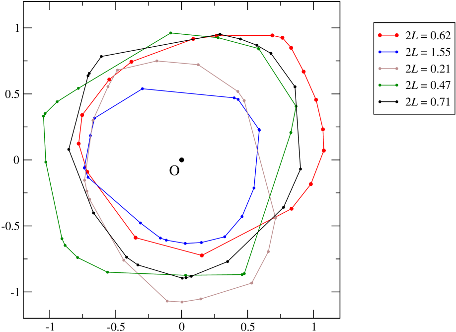
Figure 5: Five $18$-sided cell faces found in the Monte Carlo simulations of Ref. [7], superposed such that their origins coincide in a single point $\mathbf{O}$. For each, the value $2L$ of the distance between the two focal seeds is indicated.

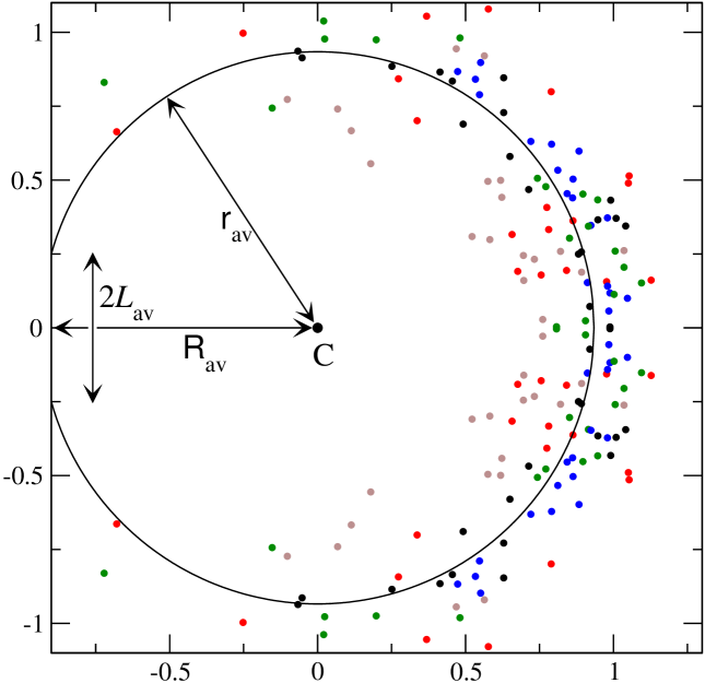
Figure 6: Figure based on the same five $18$-sided cell faces as shown in figure 5, with the same color code. All $5\times 18$ first-neighbor planes have been superposed such that the $z$ axes remain parallel and the $\mathbf{C}_{m}$ coincide in a single point $\mathbf{C}$, taken here as the origin of the coordinate system. The dots represent points of polar coordinates $(r_{m},\theta_{m})$, defined in figure 3. In order to symmetrize the figure the points $(r_{m},-\theta_{m})$ are also shown. The hull of a spindle torus, indicated by the circular arc, becomes clearly visible. See text.

4.2 Average area $A_{n}$ and perimeter $P_{n}$

In figure 7 we have represented our Monte Carlo averages $A_{n_{E}}^{\rm MC}$ and $P_{n_{E}}^{\rm MC}$ for the area and perimeter, respectively, of the ${n_{E}}$-edged cell face, averaged over the set of $4\times 10^{9}$ cells. Each quantity has been divided by its theoretical large-${n_{E}}$ behavior (3.25), so that for both the data points are expected to tend to unity as ${n_{E}}\to\infty$. We emphasize again that the theory has no adjustable parameters. The data for $A_{n_{E}}^{\rm MC}$ and $P_{n_{E}}^{\rm MC}$ appear to fully conform to the theoretical prediction, even if the finite-${n_{E}}$ corrections are still large. We will analyze these subleading terms to the asymptotic laws in section 5.

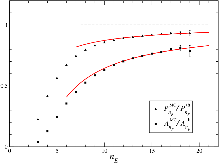
Figure 7: Monte Carlo averages $A_{n_{E}}^{\rm MC}$ and $P_{n_{E}}^{\rm MC}$ of the area and perimeter, respectively, of an ${n_{E}}$-edged cell face, each divided by its theoretical asymptotic behavior, Eqs. (3.25). Both sets of data points are predicted, therefore, to tend to unity as ${n_{E}}\to\infty$. The solid red lines approach this limit value as $\sim n^{-1}$ and represent our best estimates for the next-order correction to the leading asymptotic behavior (section 5).

4.3 Focal distance $L$

As far as we are aware, the statistics of the focal distance $L$ for given edgedness ${n_{E}}$ has not hitherto received any attention in the literature, whether it be its average $L_{n_{E}}$ or its full probability distribution $Q_{n_{E}}(L/L_{n_{E}}^{\rm th})$. The theoretical result of Eq. (3.22) for $L_{n_{E}}$ is not intuitive and it is therefore of utmost importance that we compare the predictions (3.22) and (3.18) to the Monte Carlo data.

In figure 8 we have represented the Monte Carlo average $L_{n_{E}}^{\rm MC}$, divided by its theoretical large-${n_{E}}$ behavior (3.22), so that the data points are expected to tend to unity for ${n_{E}}\to\infty$. The Monte Carlo data are fully compatible with the asymptotic limit value, even though there appear, here as before, sizeable finite-${n_{E}}$ corrections.

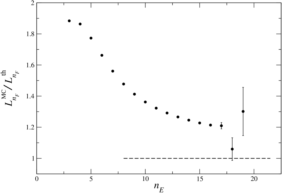
Figure 8: Monte Carlo average $L_{n_{E}}^{\rm MC}$ of the focal distance divided by its theoretical asymptotic behavior (3.22). The data points are, therefore, predicted to tend to unity as ${n_{E}}\to\infty$.

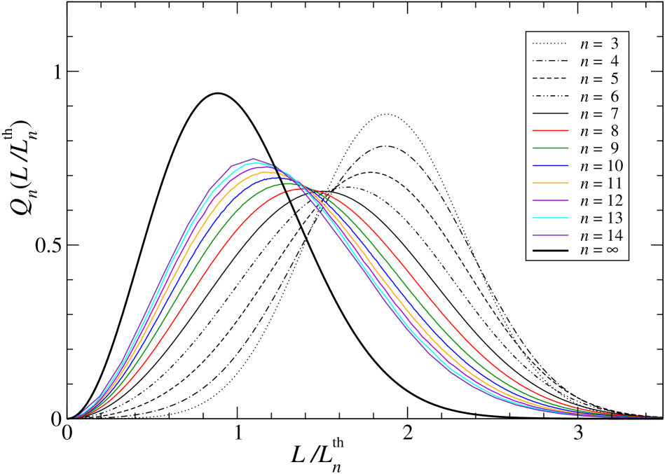
Figure 9: Monte Carlo data for the probability distributions $Q_{n}(L/L_{n}^{\rm th})$ of the focal distance $L$. The heavy black curve is the theoretical limit distribution $Q(y)$ of Eq. (3.18).

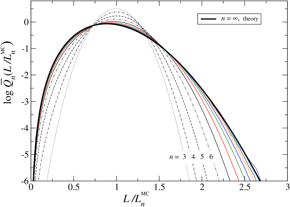
Figure 10: Monte Carlo data for the logarithm of the scaled probability distributions $\bar{Q}_{n}(L/L_{n}^{\rm MC})$ of the focal distance $L$. The color code is as in figure 9; the curves for $n=3,4,5,6$ have been labeled explicitly. These distributions all have unit average. The heavy black curve is the theoretical limit distribution $\log Q(y)$ of Eq. (3.18).

In figure 9 we proceed to a more detailed comparison. This figure shows, for $n=7$ through $n=14$, the distributions $Q_{n}(L/L_{n}^{\rm th})$ of the scaled variables $L/L_{n}^{\rm th}$. We constructed this figure by collecting the values of $L$ for each $n$ separately in bins of width $0.005$. In order to suppress fluctuations, we combined for the larger $n$ values groups of neighboring bins into larger ones: for $n=11,12,13,14$ we grouped together $2,4,8,16$ of the original bins, respectively. There is a clear tendency for the $Q_{n}(y)$ to approach the theoretical limit distribution.

In figure 10 we investigate the shape  of the distributions $Q_{n}(y)$. Let $\alpha=L_{n}^{\rm th}/L_{n}^{\rm MC}$ and define rescaled distributions $\bar{Q}_{n}(L/L_{n}^{\rm MC})=\alpha Q_{n}(y)$, which have unit average. We have plotted the $\bar{Q}_{n}$ semilogarithmically to allow for comparisons over a wider range of the abscissa. It appears that the shape of the $\bar{Q}_{n}$ converges rapidly to the theoretically predicted limit given by Eq. (3.18). Hence the limiting shape of the distribution is attained well before the average reaches its limit value. This excellent agreement comes somewhat as a surprise since we had no specific reasons beforehand to expect it.

In any case, the Monte Carlo data for $L$ provide ample evidence of the fact that ${L}_{n_{E}}/{\sf r}_{n_{E}}\to 0$ as ${n_{E}}\to\infty$, and that therefore the limit torus has equal major and minor radii: it is a true doughnut but with a hole of zero diameter.

5 Higher order terms

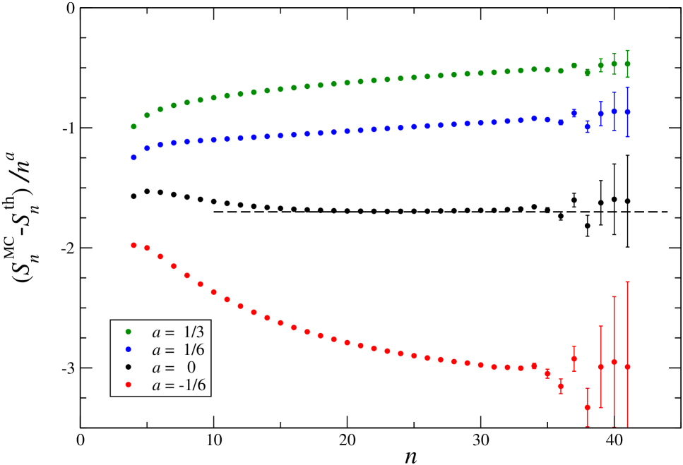
Figure 11: Trying to fit the next-to-leading term in the asymptotic expansion of $S_{n}$ by different powers $a$. From top to bottom $a=\tfrac{1}{3},\tfrac{1}{6},0,-\tfrac{1}{6}$.

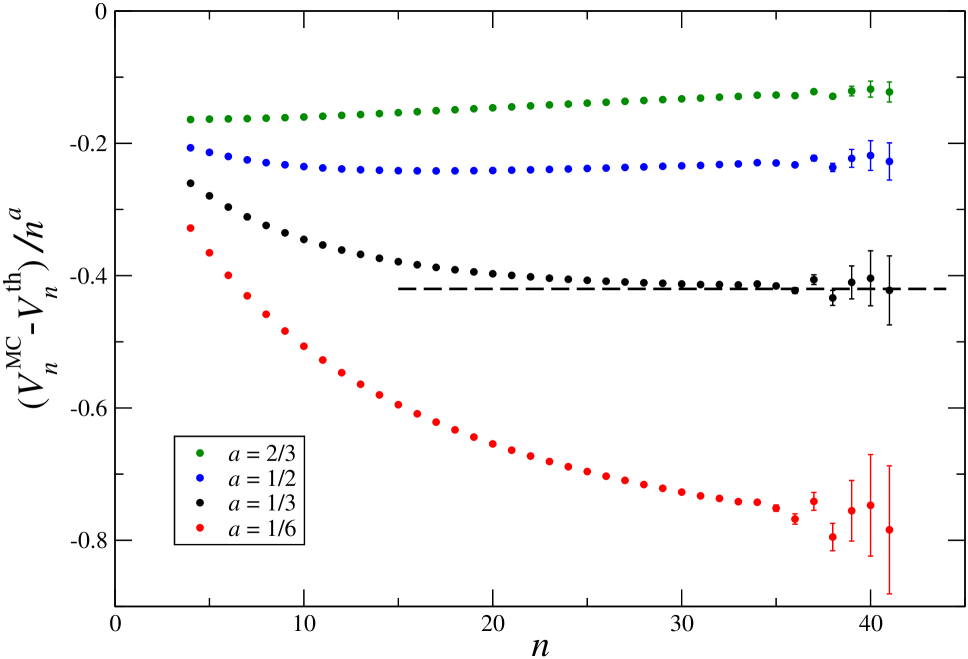
Figure 12: Trying to fit the next-to-leading term in the asymptotic expansion of $V_{n}$ by different powers $a$. From top to bottom $a=\tfrac{2}{3},\tfrac{1}{2},\tfrac{1}{3},\tfrac{1}{6}$.

We will let $n$ stand for either ${n_{E}}$ or ${n_{F}}$, and $X_{n}$ for any of the four quantities $V_{n},S_{n},A_{n}$, and $P_{n}$ studied in the preceding sections. We there determined their leading large-$n$ behavior $X_{n}^{\rm th}\simeq c_{0}n^{a_{0}}$, and now ask if we can go beyond that. Each of these averages presumably has an asymptotic expansion in powers $n$ of the form

$$X_{n}=c_{0}n^{a_{0}}+c_{1}n^{a_{1}}+\ldots,\qquad n\to\infty,$$ (5.1)

with coefficients $c_{1},c_{2},\ldots$ and powers $a_{1},a_{2},\ldots$ of which we have no theoretical knowledge. We will nevertheless rely on the idea that the only powers that one may reasonably expect are powers of $n^{1/3}$. We will try to determine these from the Monte Carlo data. Our procedure will follow the definition of an asymptotic expansion: We plot $(X_{n}^{\rm MC}-X_{n}^{\rm th})/n^{a}$ for selected values of $a$ and look for the $a$ that makes this quantity tend to a constant when $n$ gets large. That value of $a$ is then equal to $a_{1}$ and the constant is equal to $c_{1}$. How well this works depends in part on the accuracy of the simulation data, and in part on whether we are sufficiently far in the asymptotic regime, a question to which we have no certain answer.

Let us consider first the $n$-faced cell. The most clearcut case is provided by its surface area $S_{n}$, plotted in figure 11 for a selection of values of $a$ that also include half-integer powers of $n^{1/3}$. This plot seems to clearly single out $a=a_{1}=0$ as the next exponent in the series (5.1) for $X_{n}=S_{n}$. Accepting this exponent value we are led to conclude that the corresponding constant takes the value $c_{1}=-1.70$, indicated by the horizontal dashed line in the figure. In figure 12 a similar analysis has been performed for $V_{n}$. It points towards an exponent $a_{1}=1/3$ and a coefficient $c_{1}=-0.42$. The resulting two-term asymptotic series for $V_{n_{F}}$ and $S_{n_{F}}$ have been listed in table 3. The curve representing the subleading term has been drawn in figure 1 for both quantities.

Quantity	Symbol	Leading term(s) for large $n$	Note
Average surface area of an $n$-faced 3D cell	$S_{n}$	$({9\pi}/{16})^{1/3}n^{2/3}-1.70$	a
Average volume of an $n$-faced 3D cell	$V_{n}$	$n/8-0.42n^{1/3}$	a
Average perimeter of an $n$-edged face of a 3D cell	$P_{n}$	$(4\pi)^{1/3}n^{1/3}-2.95n^{-2/3}$	a
Average area of an $n$-edged face of a 3D cell	$A_{n}$	$(4\pi)^{-1/3}n^{2/3}-1.53n^{-1/3}$	a
Average of the distance $L$ between the seeds of
two 3D cells sharing an $n$-edged face	$L_{n}$	$2^{5/3}3^{-1/2}\pi^{-7/6}n^{-1/6}$	b
Probability distribution of $y=L/L_{n}$	$Q(y)$	$32\pi^{-2}y^{2}\exp(-4y^{2}/\pi)$	b
Average perimeter of an $n$-sided 2D cell	$P^{(2)}_{n}$	$\pi^{1/2}n^{1/2}-(5/8)\pi^{1/2}n^{-1/2}$	c
Average area of an $n$-sided 2D cell	$A^{(2)}_{n}$	$n/4-0.6815$	c

^a This work. First term from large-$n$ theory, expected to be exact; second term fitted.
^b This work. Leading order term from large-$n$ theory.
^c First term analytically exact [4]; second term from a high precision fit [13].

Table 3: Summary of predictions for the asymptotic large-$n$ behavior of several quantities associated with Poisson-Voronoi tessellations. The last two lines concern earlier work.

Let us next consider the average perimeter $P_{n}$ and area $A_{n}$ of an $n$-edged face. Figures 13 and 14 show the attempts to fit the asymptotic behavior. The evidence is less convincing here than for the case of the cell volume and surface area, and it certainly helps to assume at this point that the exponents are quantized as multiples of $1/3$. The values $a_{1}=-2/3$ for $P_{n}$ and $a_{1}=-1/3$ for $A_{n}$ appear to best fit the data, and accepting these we obtain estimates for the coefficients, again indicatd by horizontal dashed lines. The resulting two-term asymptotic series for $P_{n}$ and $A_{n}$ have also been listed in table 3. The curve representing the subleading term has been drawn in figure 7 for both quantities.

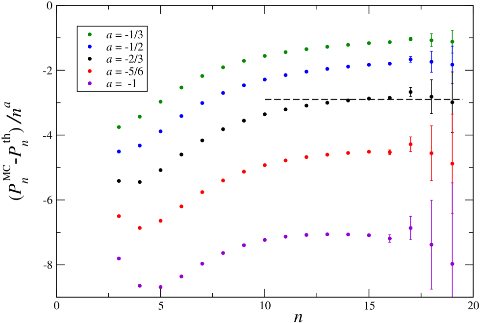
Figure 13: Trying to fit the next-to-leading term in the asymptotic expansion of $P_{n}$ by different powers $a$. From top to bottom $a=-\tfrac{1}{3},-\tfrac{1}{2},-\tfrac{2}{3},-\tfrac{5}{6}$, -$1$.

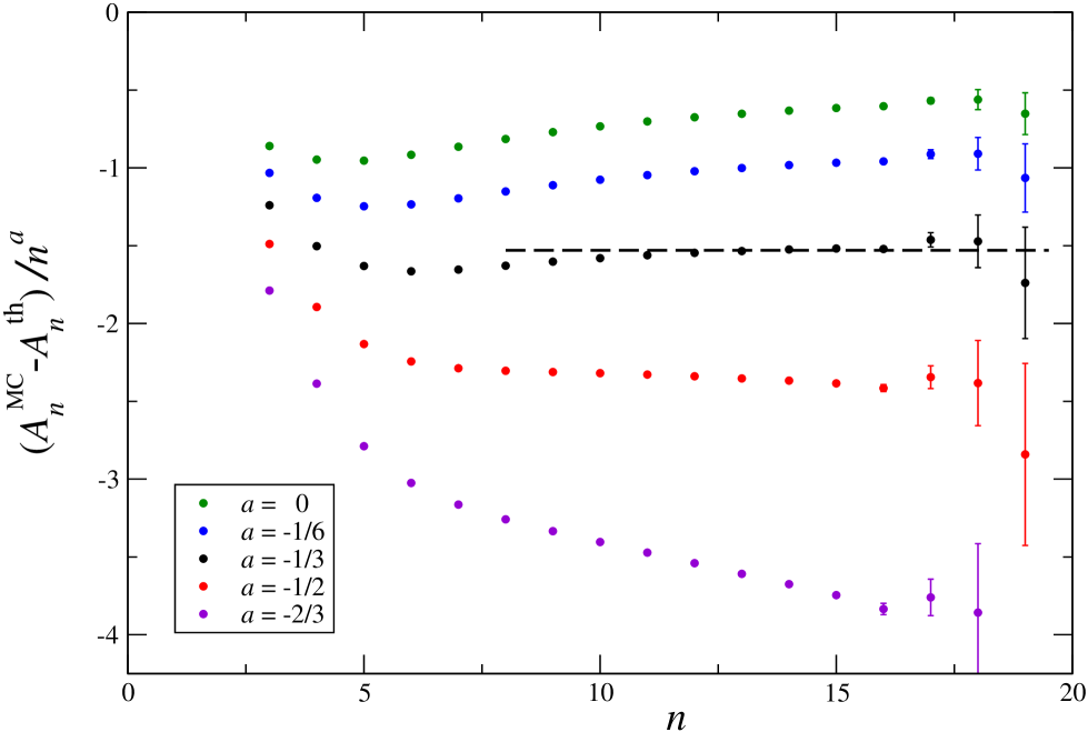
Figure 14: Trying to fit the next-to-leading term in the asymptotic expansion of $A_{n}$ by different powers $a$. From top to bottom $a=0,-\tfrac{1}{6},-\tfrac{1}{3},-\tfrac{1}{2},-\tfrac{2}{3}$.

6 Discussion

We have summarized the main results of this paper in table 3. For comparison the two bottom lines in this table show analogous results obtained earlier [4, 13] for the average perimeter $P^{(2)}_{n}$ and area $A^{(2)}_{n}$ of a two-dimensional Poisson-Voronoi cell. The status of these results, briefly indicated in the notes at the bottom of the table, is as follows. We basically have two reasons to believe that in three dimensions the results from large-$n$ theory are exact for the four quantities $V_{n}$, $S_{n}$, $A_{n}$, and $P_{n}$. The first reason is that in two dimensions this theory reproduces the exactly known leading order results for $A_{n}^{(2)}$ and $P_{n}^{(2)}$. The second one is that the theory leads to what looks like a sound basic principle: The probability of occurrence (entropy) of an “event” imposing restrictions on the positions of $n$ seeds is maximized by displacing (with respect to a random configuration) only those $n$ seeds, thus evacuating a spatial region of volume $n/\lambda$ (where $\lambda$ is the seed density). For the $n$-faced cell this region is a sphere [Eq. (2.1)], for the $n$-edged face it is a torus [Eq. (3.14)] with major and minor radii that for $n\to\infty$ become equal.

Large-$n$ theory, at least in its present form, does not allow for a systematic expansion of the averages considered above in negative powers of $n$. We have therefore based our determination of the correction terms on fits of the Monte Carlo data, guided by theoretical considerations. In next-to-leading order there is in each case a power of $n$ and a coefficient to estimate. In the case of $V_{n}$ and $S_{n}$ these come out fairly unambiguously. In the case of $A_{n}$ and $P_{n}$ we have been led, in addition, by a certain systematics that appears: just like $A_{n}^{(2)}$ and $P_{n}^{(2)}$ in two dimensions, and for reasons that we do not at this point fully understand, the correction terms for $A_{n}$ and $P_{n}$ turn out to differ from the leading order behavior by integer powers of $n^{-1}$.

The focal distance $L$ is a quantity that enters in a different way into the theory. First, in contradistinction to the four averages discussed above, its theoretical mean value $L^{\rm th}_{n}$ does not diverge with growing $n$ but tends to zero as $\sim n^{-1/6}$. The Monte Carlo data for $L^{\rm MC}_{n}$ are fully compatible with this prediction; there are again substantial finite-$n$ corrections which, in this quantity, we have not attempted to estimate. Secondly, it appears that even for large $n$ the probability distribution $Q_{n}$ of the scaled variable $y=L/L^{\rm th}_{n}$ does not become sharply peaked but approaches a well-defined limit law $Q(y)$ [Eq. (3.18)]. Although we had no a priori  indication about the reliability of these conclusions from large-$n$ theory, the distribution $Q(y)$ appears to be in excellent agreement with theory.

From the theoretical point of view it is worthwhile to recall an invariance property exploited in section 3.3, viz. the fact that a cell face does not change when any or all of the first neighbors (to its two focal seeds) are rotated over arbitrary angles in their ‘first-neighbor’ planes. We suspect that this invariance may open the road to an exact determination of the properties of the many-sided cell face.

7 Conclusion

We have performed and theoretically analyzed Monte Carlo simulations of three-dimensional Poisson-Voronoi cells. The number of cells generated, namely equals $4\times 10^{9}$, is larger than in all earlier work. Our method of analysis has been the heuristic ‘large-$n$’ theory, applicable to Voronoi cells with a large number ${n_{F}}$ of faces, and to cell faces with a large number ${n_{E}}$ of edges. The latter application has required a substantial extension of the theory that we describe in this paper. Whereas many-faced cells must be analyzed in terms of a spherical geometry, we found that the many-edged cell face requires the geometry of a spindle torus. The squared major and minor radii of that torus differ by $L^{2}$, where the ‘focal’ distance $L$ is half the distance between the seeds of the two cells sharing that face. We were natuarally led to investigate the statistics of $L$ and found again good agreement between theory and Monte Carlo data.

The results presented here highlight, in addition, the potential use of Monte Carlo simulations in conjunction with large-$n$ theory as a means of gaining insight into the properties of 3D Poisson-Voronoi cells.

References

- [1] A. Okabe, B. Boots, K. Sugihara, and S.N. Chiu, Spatial tessellations: concepts and applications of Voronoi diagrams, second edition (John Wiley & Sons Ltd., Chichester, 2000).
- [2] J.L. Meijering, Philips Research Reports 8, 270 (1953).
- [3] H.J. Hilhorst, J. Stat. Mech. L02003 (2005).
- [4] H.J. Hilhorst, J. Stat. Mech. P09005 (2005).
- [5] H.J. Hilhorst, J. Stat. Mech. P08003 (2009).
- [6] J.K. Mason, E.A. Lazar, R.D. MacPherson, and D.J. Srolovitz, Phys. Rev. E 86, 051128 (2012).
- [7] E.A. Lazar, J.K. Mason, R.D. MacPherson, and D.J. Srolovitz, Phys. Rev. E 88, 063309 (2013).
- [8] http://web.math.princeton.edu/~lazar/voronoi.html
-
[9]
K.A. Brakke, unpublished. Available on
http://www.susqu.edu/brakke/papers/voronoi.htm - [10] P. Calka and T. Schreiber, Ann. Probab. 33, 1625 (2005).
- [11] D. Hug and R. Schneider, Geom. Funct. Anal. 17, 156 (2007).
- [12] F.T. Lewis, Anatomical Records 38, 341 (1928); 47, 59 (1930); 50, 235 (1931).
- [13] H.J. Hilhorst, J. Phys. A 40, 2615 (2007).