The 2D $\kappa$-Dirac oscillator

Abstract

In this Letter, 2D Dirac oscillator in the quantum deformed framework generated by the $\kappa$-Poincaré-Hopf algebra is considered. The problem is formulated using the $\kappa$-deformed Dirac equation. The resulting theory reveals that the energies and wave functions of the oscillator are modified by the deformation parameter.

1 Introduction

The Dirac oscillator, established in 1989 by Moshinsky and Szczepaniak [1, 2], is considered a natural framework to access the relativistic quantum properties of quantum harmonic oscillator-like systems. This model has inspired a great deal of investigations in recent years. These studies have allowed the exploration of new models in theoretical and experimental physics. In the context of recent investigations, the interest in this issue appears, for example, in quantum optics [3, 4], deformed Kempf algebra [5], graphene physics [6], noncommutative space [7, 8, 9], quantum phase transition [10, 11] and topological defects [12, 13]. Among several recent contributions on the Dirac oscillator, we refer to its first experimental verification [14]. For a more detailed approach of the Dirac oscillator see Refs. [15, 16, 17, 18, 19, 20, 21].

The dynamics of the Dirac oscillator is governed by the Dirac equation with the nonminimal prescription

$$\mathbf{p}\rightarrow\mathbf{p}-im\omega\tilde{\beta}\mathbf{r},$$ (1)

where $\mathbf{p}$ is the momentum operator, $m$ is the mass, $\omega$ the frequency of the oscillator and $\mathbf{r}$ is the position vector. In the same context, another usual framework where one can study the dynamics of the Dirac oscillator is that in connection with the theory of quantum deformations. These quantum deformations are realized based on the $\kappa$-Poincaré-Hopf algebra [22, 23, 24, 25] and has direct implications on the quantum dynamics of relativistic and nonrelativistic quantum systems. The deformation parameter $\kappa$ appearing in the theory is usually interpreted as being the Planck mass $m_{P}$ [26]. Some important contributions on $\kappa$-deformation have been studied in Refs. [27, 28, 29, 30, 31, 32, 33, 34, 35, 36, 37, 38, 39, 40].

The physical properties of $\kappa$-deformed relativistic quantum systems can be accessed by solving the $\kappa$-deformed Dirac equation [41, 42]. Recently, some studies involving $\kappa$-deformation have also been reported with great interest. Some theoretical contributions in this context can be found, for example, in Refs. [43, 44, 45, 46, 47]. The 3D Dirac oscillator has been discussed in connection with the theory of quantum deformations in Ref. [48]. However, it is well known that the 2D Dirac oscillator exhibits a dynamics completely different from that of 3D one. In this context, the main goal of this Letter is study the dynamics of the 2D Dirac oscillator in the quantum deformed framework generated by the $\kappa$-Poincaré-Hopf algebra and after compare with the usual (undeformed) 2D Dirac oscillator.

This Letter is organized as follow. In Section 2, we revise the 2D Dirac oscillator and determine the energy levels and wave functions. In Section 3, the 2D Dirac oscillator in the framework of the quantum deformation is discussed. A brief conclusion is outlined in Section 4.

2 The 2D Dirac oscillator

In this section, we briefly discuss the usual 2D Dirac oscillator for later comparison with the deformed one. One begins by writing the Dirac equation for the four-component spinor $\Psi$

$$\left(\tilde{\beta}\tilde{\boldsymbol{\gamma}}\cdot\mathbf{p}+\tilde{\beta}m\right)\Psi=E\Psi.$$ (2)

The 2D Dirac oscillator is obtained throught the nonmininal prescription in Eq. (1) where $\mathbf{r}=(x,y)$ is the position vector. We shall now make use of the underlying symmetry of the system to reduce the four-component Dirac equation to a two-component spinor equation. We use the following representation for the $\tilde{\gamma}$ matrices [49, 50, 51]

$$\tilde{\beta}=\tilde{\gamma}_{0}=\left(\begin{array}[]{cc}\sigma_{z}&0\\ 0&-\sigma_{z}\end{array}\right), \qquad\tilde{\gamma}_{1}=\left(\begin{array}[]{cc}i\sigma_{y}&0\\ 0&-i\sigma_{y}\end{array}\right),$$ (7)

$$\tilde{\gamma}_{2}=\left(\begin{array}[]{cc}-i\sigma_{x}&0\\ 0&i\sigma_{x}\end{array}\right), \qquad\tilde{\gamma}_{3}=\left(\begin{array}[]{cc}0&1\\ -1&0\end{array}\right),$$ (12)

where $\sigma_{i}$ are the Pauli matrices.

The 2D Dirac oscillator being independent of the $z$ direction, allow us decouple the usual four-component Dirac equation (2) into two two-component equations

$$H_{0}\psi=\left[\beta\gamma\cdot(\mathbf{p}-im\omega\beta\mathbf{r})+\beta m\right]\psi=E\psi,$$ (13)

where $\psi$ is a two-component spinor and the three-dimensional $\gamma$ matrices are [52, 53]

$$\beta=\gamma_{0}=\sigma_{z},\qquad\gamma_{1}=i\sigma_{y},\qquad\gamma_{2}=-is\sigma_{x},$$ (14)

where the parameter $s$, which is twice the spin value, can be introduced to characterize the two spin states [54], with $s=+1$ for spin “up” and $s=-1$ for spin “down”. By squaring Eq. (13), one obtains

$$\left[p^{2}+m^{2}\omega^{2}r^{2}-2m\omega(\sigma^{3}+sL_{3})\right]\psi=(E^{2}-m^{2})\psi.$$ (15)

If one adopts the following decomposition

$$\psi=\left(\begin{array}[]{c}\psi_{1}\\ \psi_{2}\end{array}\right)=\left(\begin{array}[]{c}f(r)\;e^{il\phi}\\ ig(r)\;e^{i(l+s)\phi}\end{array}\right),$$ (16)

for the spinor, from Eq. (15), it is possible to obtain the energy spectrum [21]:

$$E=\pm\sqrt{m^{2}+2m\omega\left(2n+|l|-sl\right)},$$ (17)

and unnormalized wave functions

$$f(\rho)=\rho^{(|l|+1)/2}e^{-\rho/2}\;M\left(-n,1+|l|,\rho\right).$$ (18)

Here, $n=0,1,2,\ldots$, $l=0,\pm 1,\pm 2,\ldots$, $\rho=m\omega r^{2}$ and $M(z)$ is the confluent hypergeometric function of the first kind [55]. It should be noted that the spectrum is spin dependent, and for $sl>0$ the energy eigenvalues are independent of $l$ as depicted in the Fig. 1.

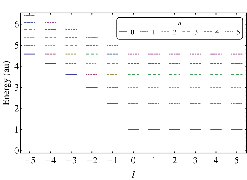
Figure 1: (Color online) The positive energy spectrum, Eq. (17), for the 2D Dirac oscillator for different values of $n$ and $l$ with $m=\omega=1$ and $s=1$. Notice that levels with quantum numbers $n\pm q$ have the same energy as levels with $l\pm q$, with $q$ an integer.

3 The 2D $\kappa$-Dirac Oscillator

In this section, we address the 2D Dirac oscillator in the framework of $\kappa$-Poincaré-Hopf algebra. We begin with the $\kappa$-Dirac equation defined in [41, 42, 46] when the third spatial coordinate is absent. So, using the same reasoning of the previous section we have

$$\left\{\gamma_{0}P_{0}-\gamma_{i}P_{i}+\frac{\varepsilon}{2}\left[\gamma_{0}(P_{0}^{2}-P_{i}P_{i})-mP_{0}\right]\right\}\psi=m\psi,$$ (19)

with $i=1,2$. Identifying $P_{0}=H=E$ and $P_{i}=\pi_{i}=p_{i}-im\omega\beta r_{i}$, we have

$$H\psi=\left[H_{0}-\frac{\varepsilon}{2}(H^{2}-\pi_{i}\pi_{i}-m\beta H)\right]\psi=E\psi,$$ (20)

By iterating Eq. (20), we have up to $\mathcal{O}(\varepsilon)$ ($\varepsilon^{2}\approx 0$)

$$H\psi=\left[H_{0}-\frac{\varepsilon}{2}(H_{0}^{2}-\pi_{i}\pi_{i}-m\beta H_{0})\right]\psi=E\psi,$$ (21)

with $H_{0}$ given in Eq. (13). By using the same representation of the previous section for the $\gamma$ matrices, Eq. (21) assumes the form

$$\left(1+\frac{m\varepsilon}{2}\sigma_{z}\right)(\sigma_{x}\pi_{x}+s\sigma_{y}\pi_{y}+m\sigma_{z})\psi=\\ \left\{E+\varepsilon\left[m^{2}\omega^{2}r^{2}-m\omega sL_{z}+im\omega\sigma_{z}(\mathbf{r}\cdot\mathbf{p})\right]\right\}\psi.$$ (22)

Equation (22), in polar coordinates $(r,\phi)$, reads

$$e^{is\sigma_{z}\phi}\left(1+\frac{m\varepsilon}{2}\sigma_{z}\right)\left[\sigma_{x}\partial_{r}+\sigma_{y}\left(\frac{s}{r}\partial_{\phi}-im\omega r\right)\right]\psi=\\ i\left[E-m\sigma_{z}+\varepsilon\left(m^{2}\omega^{2}r^{2}+im\omega s\partial_{\phi}+m\omega\sigma_{z}r\partial_{r}\right)\right]\psi.$$ (23)

Our task now is solve Eq. (23). As the deformation does not break the angular symmetry, then we can use a similar ansatz as for the usual (undeformed) case

$$\psi=\left(\begin{array}[]{c}f_{\varepsilon}(r)\;e^{il\phi}\\ ig_{\varepsilon}(r)\;e^{i(l+s)\phi}\end{array}\right),$$ (24)

but now with the radial part labeled by the deformation parameter. So, by using the ansatz (24) into Eq. (23), we find a set of two coupled radial differential equations of first order

$$\left(1+\frac{m\varepsilon}{2}\right)\left[\frac{d}{dr}+\frac{s(l+s)}{r}-m\omega r\right]g_{\varepsilon}(r)=(E-m)f_{\varepsilon}(r)\\ +\varepsilon\left(m^{2}\omega^{2}r^{2}-m\omega sl+m\omega r\frac{d}{dr}\right)f_{\varepsilon}(r),$$ (25a)

$$\left(1-\frac{m\varepsilon}{2}\right)\left[\frac{d}{dr}-\frac{sl}{r}+m\omega r\right]f_{\varepsilon}(r)=-(E+m)g_{\varepsilon}(r)\\ -\varepsilon\left(m^{2}\omega^{2}r^{2}-m\omega s(l+s)-m\omega\rho\frac{d}{dr}\right)g_{\varepsilon}(r).$$ (25b)

The above system of equations can be decoupled yielding a single second order differential equation for $f_{\varepsilon}(r)$,

$$-f_{\varepsilon}^{\prime\prime}(r)-\left(\frac{1}{r}+2m^{2}\varepsilon\omega r\right)f_{\varepsilon}^{\prime}(r)\\ +\left[\frac{l^{2}}{r^{2}}+\left(1-2E\varepsilon\right)m^{2}\omega^{2}r^{2}-k_{\varepsilon}^{2}\right]f_{\varepsilon}(r)=0,$$ (26)

where

$$k_{\varepsilon}^{2}=E^{2}-m^{2}+2m\omega\left[(sl+1)(1-\varepsilon E)+m\varepsilon\right].$$ (27)

A similar equation for $g_{\varepsilon}$ there exists. The regular solution for Eq. (26) is

$$f_{\varepsilon}(\rho)=(\lambda_{\varepsilon}\;\rho)^{(|l|-1)/2}e^{-(m\varepsilon+\lambda_{\varepsilon})\rho/2}M\left(d_{\varepsilon},1+|l|,\lambda_{\varepsilon}\;\rho\right),$$ (28)

where

$$\lambda_{\varepsilon}=1-E\varepsilon,$$ (29)

and

$$d_{\varepsilon}=\frac{1+|l|}{2}+\frac{2m^{2}\omega\varepsilon-k_{\varepsilon}^{2}}{4\gamma\lambda_{\varepsilon}}.$$ (30)

The deformed spectrum are obtained by establishing as convergence criterion the condition $d_{\varepsilon}=-n$. In this manner, the deformed energy spectrum is given by

$$E^{2}-m^{2}=2m\omega(2n+|l|-sl)\lambda_{\varepsilon}.$$ (31)

Thus, solving Eq. (31) for $E$, the deformed energy levels are explicitly given by

$$E=\pm\sqrt{m^{2}+2m\omega\left(2n+|l|-sl\right)}-m\varepsilon\omega(2n+|l|-sl),$$ (32)

and its unnormalized wave functions are of the form

$$f_{\varepsilon}(\rho)=(\lambda_{\varepsilon}\;\rho)^{(|l|-1)/2}e^{-(m\varepsilon+\lambda_{\varepsilon})\rho/2}M\left(-n,1+|l|,\lambda_{\varepsilon}\;\rho\right).$$ (33)

In deriving our results we have neglected terms of $O(\varepsilon^{2})$.

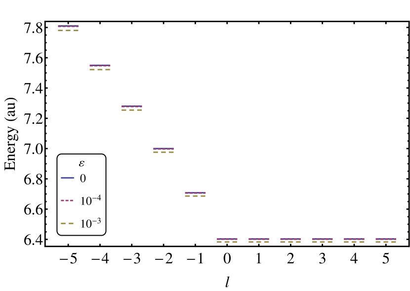
Figure 2: (Color online) The deformed energy levels, Eq. (32), for the 2D $\kappa$-Dirac oscillator for $n=10$, $s=1$ and for different values of $l$. We use units such as $m=\omega=1$.

We can observe that the particle and antiparticle energies in the 2D $\kappa$-Dirac oscillator are different, as a consequence of charge conjugation symmetry breaking caused by the deformation parameter in the same manner as observed in the three-dimensional one [48]. Notice that, $\varepsilon=0$, exactly conducts to the results for the energy levels and wave functions of the previous section for the usual (undeformed) 2D Dirac oscillator, revealing the consistency of the description here developed. It is worthwhile to note that the infinity degeneracy present in the usual two-dimensional Dirac oscillator is preserved by the deformation, but affecting the separation of the energy levels. The distance between the adjacent energy levels decreases as the deformation parameter increases. In Fig. 2 is depicted the undeformed and deformed energy levels for some values of the deformation parameter for $n=10$. In Ref. [43], we have determined a upper bound for the deformation parameter. Taking into account this upper bound, the product $m\varepsilon$ should be smaller than $0.00116$. In this manner, using units such as $m=1$, we must consider values for the deformation smaller than $0.00116$.

4 Conclusions

In this letter, we considered the dynamics of the 2D Dirac oscillator in the context of $\kappa$-Poincaré-Hopf algebra. Using the fact that the deformation does not break the angular symmetry, we have derived the $\kappa$-deformed radial differential equation whose solution has led to the deformed energy spectrum and wave functions. We verify that the energy spectrum and wave functions are modified by the presence of the deformation parameter $\varepsilon$. Using values for the deformation parameter lower than the upper bound $0.00116$, we have examined the dependence of the energy of the oscillator with the deformation. The deformation parameter modifies the energy spectrum and wave functions the Dirac oscillator, preserving the infinity degeneracy, but affecting the distance between the adjacent energy levels. Finally, the case $\varepsilon=0$, exactly conducts for the results for the usual 2D Dirac oscillator.

5 Acknowledgments

We would like to thank Rodolfo Casana for discussions on dimensionality of the deformed Dirac equation. This work was supported by the Fundação Araucária (Grant No. 205/2013 (PPP) and No. 484/2014 (PQ)), and the Conselho Nacional de Desenvolvimento Científico e Tecnológico (Grants No. 482015/2013-6 (Universal), No. 306068/2013-3 (PQ)) and FAPEMA (Grant No. 00845/13).

References

- Moshinsky and Szczepaniak [1989] M. Moshinsky, A. Szczepaniak, J. Phys. A 22 (1989) L817–. doi:10.1088/0305-4470/22/17/002.
- Moshinsky and Smirnov [1996] M. Moshinsky, Y. Smirnov, The Harmonic Oscillator in Modern Physics, Contemporary concepts in physics, Harwood Academic Publishers, 1996. URL: http://books.google.com.br/books?id=RA-xtOg4z90C.
- Bermudez et al. [2007] A. Bermudez, M. A. Martin-Delgado, E. Solano, Phys. Rev. A 76 (2007) 041801. doi:10.1103/PhysRevA.76.041801.
- Bermudez et al. [2008] A. Bermudez, M. A. Martin-Delgado, A. Luis, Phys. Rev. A 77 (2008) 033832. doi:10.1103/PhysRevA.77.033832.
- Betrouche et al. [2013] M. Betrouche, M. Maamache, J. R. Choi, Sci. Rep. 3 (2013) 3221. doi:10.1038/srep03221.
- Quimbay and Strange [2013] C. Quimbay, P. Strange (2013). arXiv:1311.2021.
- Vega [2014] F. Vega, J. Math. Phys. 55 (2014) 032105. doi:10.1063/1.4866914.
- Maluf [2011] R. V. Maluf, Int. J. Mod. Phys. A 26 (2011) 4991. doi:10.1142/S0217751X11054887.
- Luo et al. [2012] Z.-Y. Luo, Q. Wang, X. Li, J. Jing, Int. J. Theor. Phys. 51 (2012) 2143. doi:10.1007/s10773-012-1094-x.
- Bermudez et al. [2008] A. Bermudez, M. A. Martin-Delgado, A. Luis, Phys. Rev. A 77 (2008) 063815. doi:10.1103/PhysRevA.77.063815.
- Quimbay and Strange [2013] C. Quimbay, P. Strange (2013). arXiv:1312.5251.
- Bakke and Furtado [2013] K. Bakke, C. Furtado, Ann. Phys. (NY) 336 (2013) 489. doi:10.1016/j.aop.2013.06.007.
- Carvalho et al. [2011] J. Carvalho, C. Furtado, F. Moraes, Phys. Rev. A 84 (2011) 032109. doi:10.1103/PhysRevA.84.032109.
- Franco-Villafañe et al. [2013] J. A. Franco-Villafañe, E. Sadurní, S. Barkhofen, U. Kuhl, F. Mortessagne, T. H. Seligman, Phys. Rev. Lett. 111 (2013) 170405. doi:10.1103/PhysRevLett.111.170405.
- Toyama et al. [1997] F. M. Toyama, Y. Nogami, F. A. B. Coutinho, J. Phys. A 30 (1997) 2585. doi:10.1088/0305-4470/30/7/034.
- Sadurni [2011] E. Sadurni, AIP Conf. Proc. 1334 (2011) 249--290. doi:10.1063/1.3555484. arXiv:1101.3011.
- Strange [1998] P. Strange, Relativistic Quantum Mechanics, Cambridge University Press, Cambridge, England, 1998.
- Villalba [1994] V. M. Villalba, Phys. Rev. A 49 (1994) 586. doi:10.1103/PhysRevA.49.586.
- Villalba and Rincón Maggiolo [2001] V. M. Villalba, A. Rincón Maggiolo, Eur. Phys. J. B 22 (2001) 31. doi:10.1007/BF01325457.
- Rao and Kagali [2004] N. A. Rao, B. A. Kagali, Mod. Phys. Lett. A 19 (2004) 2147. doi:10.1142/S0217732304014719.
- Andrade and Silva [2014] F. M. Andrade, E. O. Silva (2014). arXiv:1403.4113.
- Lukierski et al. [1991] J. Lukierski, H. Ruegg, A. Nowicki, V. N. Tolstoy, Phys. Lett. B 264 (1991) 331. doi:10.1016/0370-2693(91)90358-W.
- Lukierski et al. [1992] J. Lukierski, A. Nowicki, H. Ruegg, Phys. Lett. B 293 (1992) 344. doi:10.1016/0370-2693(92)90894-A.
- Lukierski and Ruegg [1994] J. Lukierski, H. Ruegg, Phys. Lett. B 329 (1994) 189. doi:10.1016/0370-2693(94)90759-5.
- Majid and Ruegg [1994] S. Majid, H. Ruegg, Phys. Lett. B 334 (1994) 348. doi:10.1016/0370-2693(94)90699-8.
- Kovacević et al. [2012] D. Kovacević, S. Meljanac, A. Pachoł, R. Štrajn, Physics Letters B 711 (2012) 122. doi:10.1016/j.physletb.2012.03.062.
- Lukierski et al. [1995] J. Lukierski, H. Ruegg, W. Zakrzewski, Ann. Phys. (NY) 243 (1995) 90. doi:10.1006/aphy.1995.1092.
- Arzano et al. [2010] M. Arzano, J. Kowalski-Glikman, A. Walkus, Class. Quantum Grav. 27 (2010) 025012.
- Kosiński et al. [2001] P. Kosiński, J. Lukierski, P. Maślanka, Nucl. Phys. B - Proc. suppl. 102-103 (2001) 161. doi:10.1016/S0920-5632(01)01552-3.
- Dimitrijević et al. [2003] M. Dimitrijević, L. Jonke, L. Möller, E. Tsouchnika, J. Wess, M. Wohlgenannt, Eur. Phys. J. C 31 (2003) 129. doi:10.1140/epjc/s2003-01309-y.
- Cougo-Pinto et al. [2002] M. Cougo-Pinto, C. Farina, J. Mendes, Phys. Lett. B 529 (2002) 256. doi:10.1016/S0370-2693(02)01253-4.
- Harikumar et al. [2011] E. Harikumar, T. Jurić, S. Meljanac, Phys. Rev. D 84 (2011) 085020. doi:10.1103/PhysRevD.84.085020.
- Dimitrijević and Jonke [2011] M. Dimitrijević, L. Jonke, J. High Energy Phys. 1112 (2011) 080. doi:10.1007/JHEP12(2011)080.
- Jurić et al. [2013] T. Jurić, S. Meljanac, R. Štrajn, Eur. Phys. J. C 73 (2013) 2472. doi:10.1140/epjc/s10052-013-2472-0.
- Borowiec and Pachol [2009] A. Borowiec, A. Pachol, Phys. Rev. D 79 (2009) 045012. doi:10.1103/PhysRevD.79.045012.
- Meljanac and Stojić [2006] S. Meljanac, M. Stojić, Eur. Phys. J. C 47 (2006) 531. doi:10.1140/epjc/s2006-02584-8.
- Meljanac et al. [2008] S. Meljanac, A. Samsarov, M. Stojić, K. S. Gupta, Eur. Phys. J. C 53 (2008) 295. doi:10.1140/epjc/s10052-007-0450-0.
- Meljanac et al. [2013] S. Meljanac, A. Pachoł, A. Samsarov, K. S. Gupta, Phys. Rev. D 87 (2013) 125009. doi:10.1103/PhysRevD.87.125009.
- Gupta et al. [2012] K. S. Gupta, S. Meljanac, A. Samsarov, Phys. Rev. D 85 (2012) 045029. doi:10.1103/PhysRevD.85.045029.
- Govindarajan et al. [2009] T. R. Govindarajan, K. S. Gupta, E. Harikumar, S. Meljanac, D. Meljanac, Phys. Rev. D 80 (2009) 025014. doi:10.1103/PhysRevD.80.025014.
- Nowicki et al. [1993] A. Nowicki, E. Sorace, M. Tarlini, Phys. Lett. B 302 (1993) 419--422. doi:10.1016/0370-2693(93)90419-I.
- Biedenharn et al. [1993] L. Biedenharn, B. Mueller, M. Tarlini, Phys. Lett. B 318 (1993) 613--616. doi:10.1016/0370-2693(93)90462-Q.
- Andrade and Silva [2013] F. M. Andrade, E. O. Silva, Phys. Lett. B 719 (2013) 467--471. doi:10.1016/j.physletb.2013.01.062.
- Roy and Roychoudhury [1994] P. Roy, R. Roychoudhury, Phys. Lett. B 339 (1994) 87. doi:10.1016/0370-2693(94)91137-1.
- Arzano and Marcianò [2007] M. Arzano, A. Marcianò, Phys. Rev. D 76 (2007) 125005. doi:10.1103/PhysRevD.76.125005.
- Roy and Roychoudhury [1995a] P. Roy, R. Roychoudhury, Phys. Lett. B 359 (1995a) 339. doi:10.1016/0370-2693(95)01079-6.
- Roy and Roychoudhury [1995b] P. Roy, R. Roychoudhury, Mod. Phys. Lett. A 10 (1995b) 1969. doi:10.1142/S0217732395002118.
- Andrade et al. [2014] F. M. Andrade, E. O. Silva, M. M. Ferreira Jr., E. C. Rodrigues, Phys. Lett. B 731 (2014) 327. doi:10.1016/j.physletb.2014.02.054.
- de Vega [1978] H. J. de Vega, Phys. Rev. D 18 (1978) 2932--2944. doi:10.1103/PhysRevD.18.2932.
- Brandenberger et al. [1988] R. H. Brandenberger, A.-C. Davis, A. M. Matheson, Nucl. Phys. B 307 (1988) 909--923. doi:10.1016/0550-3213(88)90112-5.
- Alford and Wilczek [1989] M. G. Alford, F. Wilczek, Phys. Rev. Lett. 62 (1989) 1071--1074. doi:10.1103/PhysRevLett.62.1071.
- Hagen [1990] C. R. Hagen, Phys. Rev. Lett. 64 (1990) 2347--2349. doi:10.1103/PhysRevLett.64.2347.
- Hagen [1991] C. R. Hagen, Int. J. Mod. Phys. A 6 (1991) 3119. doi:10.1142/S0217751X91001520.
- Khalilov [2014] V. Khalilov, Eur. Phys. J. C 74 (2014) 1--7--. doi:10.1140/epjc/s10052-013-2708-z.
- Abramowitz and Stegun [1972] M. Abramowitz, I. A. Stegun (Eds.), Handbook of Mathematical Functions, New York: Dover Publications, 1972.