UWThPh-2014-13
A complete survey of texture zeros
in the lepton mass matrices

Abstract

We perform a systematic and complete analysis of texture zeros in the lepton mass matrices and identify all viable and maximally restrictive cases of pairs $(M_{\ell},M_{D})$ and $(M_{\ell},M_{L})$, where $M_{\ell}$, $M_{D}$ and $M_{L}$ are the charged-lepton, Dirac neutrino and Majorana neutrino mass matrices, respectively. To this end, we perform a thorough analysis of textures which are equivalent through weak-basis permutations. Furthermore, we introduce numerical measures for the predictivity of textures and apply them to the viable and maximally restrictive texture zero models. It turns out that for Dirac neutrinos these models can at most predict the smallest neutrino mass and the CKM-type phase of the mixing matrix. For Majorana neutrinos most models can, in addition, predict the effective neutrino mass for neutrinoless double beta decay. Apart from one model, which has marginal predictive power with respect to $\sin^{2}\!\theta_{23}$, no other model can predict any of the already measured observables.

1 Introduction

In spite of the enormous progress in our knowledge of neutrino masses and lepton mixing [1, 2, 3, 4], the origin of the leptonic flavour structure is still a mystery. One popular approach to resolve this mystery is through underlying symmetries. The simplest symmetries in this context are Abelian. Such symmetries can be used to impose texture zeros in the mass matrices in order to make them predictive—see for instance [5, 6] for the lepton sector and [7] for the quark sector. Vice versa, given mass matrices with texture zeros, one can always find an extended scalar sector and suitable Abelian symmetries such that the texture zeros originate from these symmetries [8, 9]. In this sense, texture zeros are synonymous with Abelian symmetries. In the most simple scenario the charged-lepton mass matrix $M_{\ell}$ is diagonal, which signifies six texture zeros in $M_{\ell}$, and, assuming that neutrinos are Majorana fermions, some texture zeros are placed in the Majorana mass matrix $M_{L}$. It has been shown that the data allow seven mass matrices $M_{L}$ with two texture zeros [10]. Subsequently, these seven cases have received a lot of attention—see [11, 12, 13, 14, 15, 16, 17, 18, 19, 20, 21, 22, 23, 24, 25, 26] for an incomplete list of references. If neutrinos are Dirac particles, then one has more freedom for texture zeros in the corresponding mass matrix $M_{D}$ [27] because $M_{D}$ is an arbitrary complex $3\times 3$ matrix, in contrast to $M_{L}$ which has to be symmetric. As for cases with $M_{\ell}$ non-diagonal, studies are usually confined to instances where both the charged-lepton and the neutrino mass matrix have a Fritzsch-like texture [28, 29] or extensions of it—see [30, 31, 32, 33, 34, 35, 36, 37, 38, 39, 40, 41, 42, 43, 44] and references therein. In general, one can define “parallel textures” as those where $M_{\ell}$ and $M_{L}$ or $M_{D}$ have the same texture [45, 46]. For a recent review on textures we refer the reader to [47].

In this paper we perform a systematic numerical study of all possibilities of texture zeros in the charged-lepton and neutrino mass matrices. We stress that this study also includes all non-parallel textures. Moreover, we investigate both Dirac and Majorana neutrino mass matrices and for each of these two neutrino types we discuss separately normal ordering ($m_{1}<m_{2}<m_{3}$) and inverted ordering ($m_{3}<m_{1}<m_{2}$) of the neutrino mass spectrum. Our main results will be presented as four lists of viable and maximally restrictive textures, i.e. those textures with a maximal number of zeros which are able to reproduce the existing mass and mixing data. However, it is not only interesting if a texture is viable, it is also rewarding to know if a texture is predictive. In order to define such general predictivity criteria, we note that there are eight known observables $\mathcal{O}_{j}$ ($j=1,\ldots,8$) in the lepton sector, the three charged-lepton masses, the two neutrino mass-squared differences and three mixing angles, and five other observables, on which (almost) nothing is known: the smallest neutrino mass, the effective neutrino mass in neutrinoless double beta decay, the CKM-type phase and the two Majorana phases. Our predictivity criterion for the eight known observables will be defined as certain numerical measures which allow to judge how well the mean value of $\mathcal{O}_{i}$ can be predicted from the measured values $\overline{\mathcal{O}}_{j}\pm\sigma_{j}$ ($j\neq i$) of the seven other observables. A related but distinct numerical method will be applied to the five observables which have not yet been measured. The results of the predictivity analyses will be included in the lists of viable textures.

The notation of texture zeros in this paper is the usual one: texture zeros are denoted by zero entries in the mass matrix, while an entry $\times$ in a mass matrix denotes an arbitrary complex number. For example, the matrix

$$\begin{pmatrix}\times&\times&0\\ \times&0&\times\\ 0&0&\times\end{pmatrix}$$ (1)

has four texture zeros and the five entries $\times$ denote arbitrary and independent complex numbers. Majorana mass matrices are understood to be symmetric, so if

$$\begin{pmatrix}\times&\times&0\\ \times&0&0\\ 0&0&\times\end{pmatrix}$$ (2)

represents a Majorana mass matrix, the 11, 12 and 33-entries are arbitrary complex numbers, while the 21-element must be equal to the 12-element. Since this matrix contains only three independent zero entries, it is counted as an instance of three texture zeros in a Majorana mass matrix.

The paper is organized as follows. In section 2 we discuss basic constraints on the mass matrices. Section 3 is devoted to the relationship between texture zeros and weak-basis transformations. In section 4 we classify the possible inequivalent texture-zero models for Dirac and Majorana neutrinos. Section 5 is the main part of the paper: it contains the explanation of the numerical analyses, the definition of our predictivity measures and the results of our analyses. Finally, in section 6 the conclusions are presented. Some technical details of the numerics are deferred to an appendix.

2 Basic constraints on the lepton mass matrices

In this paper, one of our basic assumptions is that the lepton masses and the mixing matrix are obtained, with sufficient accuracy, by the tree-level mass matrices. Thus we require the charged-lepton mass matrix to have rank three, while the neutrino mass matrix can have rank three or two, since one neutrino mass being zero is compatible with all experimental data. For example, the mass matrix

$$\begin{pmatrix}0&0&0\\ \times&\times&\times\\ \times&\times&\times\end{pmatrix}$$ (3)

will in general have rank two and thus does not represent an acceptable charged-lepton mass matrix. However, it represents a viable Dirac neutrino mass matrix.

In the case of Majorana neutrinos there is another possible constraint. Namely, the fact that the Majorana mass matrix is symmetric, in combination with texture zeros, can lead to matrices with two equal singular values, which we exclude. An example for such a texture in a Majorana neutrino mass matrix is

$$\begin{pmatrix}0&\times&0\\ \times&0&0\\ 0&0&\times\end{pmatrix}.$$ (4)

According to this line of reasoning, the above phenomenological requirements on the fermion masses directly exclude some types of texture zeros in the fermion mass matrices. In particular, there is a maximal number of texture zeros in the mass matrices. The fermion mass terms occurring in this paper and the maximal number of texture zeros in the mass matrices are listed in table 1. Note that in our convention the chiralities in the Dirac neutrino mass term are interchanged with respect to the charged-lepton mass term.

Fermions	mass term	masses	$\text{rank}(M)$	$n_{0,\text{max}}$
Charged leptons	$-\overline{\ell_{L}}M_{\ell}\ell_{R}+\mathrm{H.c.}$	$0<m_{e}<m_{\mu}<m_{\tau}$	$3$	$6$
Dirac neutrinos	$-\overline{\nu_{R}}M_{D}\nu_{L}+\mathrm{H.c.}$	$0\leq m_{1}<m_{2}<m_{3}$ or $0\leq m_{3}<m_{1}<m_{2}$	$\geq 2$	$7$
Majorana neutrinos	$\dfrac{1}{2}\nu_{L}^{T}C^{-1}M_{L}\nu_{L}+\text{H.c.}$	$0\leq m_{1}<m_{2}<m_{3}$ or $0\leq m_{3}<m_{1}<m_{2}$	$\geq 2$	$4$

Table 1: The mass terms discussed in this paper. Since we consider only the Standard Model field content (plus three right-handed neutrinos in the case of Dirac neutrinos), all mass matrices are arbitrary complex $3\times 3$-matrices. In addition, $M_{L}$ must be symmetric. By $\text{rank}(M)$ we denote the required rank of the mass matrix $M$ and $n_{0,\text{max}}$ is the maximal number of (independent) texture zeros which can be imposed in $M$.

The mass matrices shown in table 1 are diagonalized by

$$U_{L}^{(\ell)\dagger}M_{\ell}U_{R}^{(\ell)}=\mathrm{diag}(m_{e},\,m_{\mu},\,m_{\tau}),$$ (5a)

$$U_{R}^{(\nu)\dagger}M_{D}U_{L}^{(\nu)}=\mathrm{diag}(m_{1},\,m_{2},\,m_{3}),$$ (5b)

$$U_{L}^{(\nu)T}M_{L}U_{L}^{(\nu)}=\mathrm{diag}(m_{1},\,m_{2},\,m_{3}),$$ (5c)

where $U_{L}^{(\ell)}$, $U_{R}^{(\ell)}$, $U_{L}^{(\nu)}$ and $U_{R}^{(\nu)}$ are unitary $3\times 3$ matrices. If we impose texture zeros only in $M_{\ell}$ or only in the neutrino mass matrix, i.e. $M_{D}$ in the case of Dirac and $M_{L}$ in the case of Majorana neutrinos, only one of the two matrices $U_{L}^{(\ell)}$ and $U_{L}^{(\nu)}$ is restricted. In this case there are no constraints on the lepton mixing matrix

$$U_{\text{PMNS}}=U_{L}^{(\ell)\dagger}U_{L}^{(\nu)}.$$ (6)

3 Texture zeros and weak-basis transformations

3.1 Physical implications of texture zeros

In general, we always have the freedom to perform weak-basis transformations, i.e. field redefinitions which leave the form of the gauge and kinetic terms of the Lagrangian invariant [48, 49, 45]. In this paper we have in mind models with the same fermionic gauge multiplet structure as the Standard Model. If we consider an extension of the Standard Model by three right-handed gauge-singlet neutrino fields $\nu_{R}$ and assume lepton number conservation, then neutrinos are Dirac particles and the lepton mass terms are given by

$$-(\overline{\ell_{L}}M_{\ell}\ell_{R}+\overline{\nu_{R}}M_{D}\nu_{L}+\mathrm{H.c.})$$ (7)

(see table 1). Now we perform a field redefinition

$$\ell_{L,R}=V_{L,R}^{(\ell)}\ell_{L,R}^{\prime},\quad\nu_{L,R}=V_{L,R}^{(\nu)}\nu_{L,R}^{\prime}.$$ (8)

In order to leave the kinetic terms invariant, $V_{L,R}^{(\ell)}$ and $V_{L,R}^{(\nu)}$ must be unitary and gauge invariance requires $V_{L}^{(\ell)}=V_{L}^{(\nu)}\equiv V_{L}$. In this new weak basis, the mass terms of equation (7) are given by

$$-(\overline{\ell_{L}^{\prime}}M_{\ell}^{\prime}\ell_{R}^{\prime}+\overline{\nu_{R}^{\prime}}M_{D}^{\prime}\nu_{L}^{\prime}+\mathrm{H.c.})$$ (9)

with the new mass matrices

$$M_{\ell}^{\prime}=V_{L}^{\dagger}M_{\ell}V_{R}^{(\ell)}\quad\text{and}\quad M_{D}^{\prime}=V_{R}^{(\nu)\dagger}M_{D}V_{L}.$$ (10a)

A crucial observation in the case of Dirac neutrinos is that $$V_{R}^{(\ell)} V_{R}^{(\nu)}$$ and are independent transformation matrices, which is a consequence of the assumption that the right-handed fermion fields are gauge singlets. Obviously, we do not have this freedom in the case of Majorana neutrinos, where the weak-basis transformation on the mass matrices reads

$$M_{\ell}^{\prime}=V_{L}^{\dagger}M_{\ell}V_{R}^{(\ell)}\quad\text{and}\quad M_{L}^{\prime}=V_{L}^{T}M_{L}V_{L}.$$ (10b)

The fermion masses are the singular values of the mass matrices and are thus invariant under the biunitary transformation (10). Clearly, also the lepton mixing matrix $U_{\text{PMNS}}$ is invariant under this transformation.

Consequently, whenever two types of texture zeros are related by a transformation of the form (10), they lead to the same physical constraints and are thus physically equivalent. This trivial statement has far-reaching consequences: on the one hand it allows to divide texture zero models into equivalence classes with the same physical consequences, on the other hand it relates to the existence of types of texture zeros, which do not impose any physical constraints [49, 45, 50], a fact which follows from the following well-known theorem of linear algebra.

Theorem 1.

Let $M$ be a complex $n\times n$-matrix. Then there exist unitary $n\times n$-matrices $W_{L}$, $W_{R}$, $\widetilde{W}_{L}$, $\widetilde{W}_{R}$ such that

• $W_{L}^{\dagger}M$ is an upper triangular matrix,

• $\widetilde{W}_{L}^{\dagger}M$ is a lower triangular matrix,

• $MW_{R}$ is an upper triangular matrix,

• $M\widetilde{W}_{R}$ is a lower triangular matrix.

These four statements are equivalent to the so-called QR, QL, RQ and LQ-decomposition of complex square matrices, respectively.

Indeed, theorem 1 assures us that beginning with any mass matrices $M_{\ell}$ and $M_{D}$ (but not $M_{L}$) we can always perform a weak-basis transformation (10) such that, in the new basis, the mass matrices are upper or lower triangular matrices, i.e. $M_{\ell}$ and $M_{D}$ are of the form

$$\begin{pmatrix}\times&\times&\times\\ 0&\times&\times\\ 0&0&\times\end{pmatrix}\quad\text{or}\quad\begin{pmatrix}\times&0&0\\ \times&\times&0\\ \times&\times&\times\end{pmatrix}.$$ (11)

Consequently, any type of texture zeros equivalent to one of equation (11) is equivalent to the trivial case of no imposed texture zeros at all and does not impose any physical constraints. The textures

$$\begin{split}&\begin{pmatrix}\times&\times&\times\\ 0&\times&\times\\ 0&\times&\times\end{pmatrix},\,\begin{pmatrix}\times&\times&\times\\ 0&\times&\times\\ \times&0&\times\end{pmatrix},\,\begin{pmatrix}\times&\times&\times\\ \times&\times&\times\\ 0&0&\times\end{pmatrix},\,\\ &\begin{pmatrix}\times&\times&\times\\ 0&\times&\times\\ \times&\times&\times\end{pmatrix},\,\begin{pmatrix}\times&\times&\times\\ \times&\times&\times\\ 0&\times&\times\end{pmatrix},\,\begin{pmatrix}\times&\times&\times\\ \times&\times&\times\\ \times&0&\times\end{pmatrix},\\ &\begin{pmatrix}\times&0&0\\ \times&\times&\times\\ \times&\times&\times\end{pmatrix},\,\begin{pmatrix}\times&0&\times\\ \times&\times&0\\ \times&\times&\times\end{pmatrix},\,\begin{pmatrix}\times&\times&0\\ \times&\times&0\\ \times&\times&\times\end{pmatrix},\,\\ &\begin{pmatrix}\times&0&\times\\ \times&\times&\times\\ \times&\times&\times\end{pmatrix},\,\begin{pmatrix}\times&\times&0\\ \times&\times&\times\\ \times&\times&\times\end{pmatrix},\,\begin{pmatrix}\times&\times&\times\\ \times&\times&0\\ \times&\times&\times\end{pmatrix}\end{split}$$ (12)

are even less restrictive than the ones of equation (11) and thus also do not impose any constraints on physical observables.

3.2 Equivalence of texture zeros

The number of possible cases of texture zeros which can be imposed in fermion mass matrices is huge, however, as discussed above, not all of them lead to different physical predictions. Therefore, it is useful to divide the different patterns of texture zeros into equivalence classes with respect to weak-basis transformations. Regarding the arrangement of textures into equivalence classes, we are only interested in weak-basis transformations which leave the number of texture zeros in each individual mass matrix invariant. In general the only weak-basis transformations fulfilling this requirement will be the ones where $V_{L}$, $V_{R}^{(\ell)}$ and $V_{R}^{(\nu)}$ of equation (10) are of the form $PD$, where $P$ is one of the six permutation matrices

$$\begin{split}&P_{1}=\begin{pmatrix}1&0&0\\ 0&1&0\\ 0&0&1\end{pmatrix},\quad P_{2}=\begin{pmatrix}0&1&0\\ 1&0&0\\ 0&0&1\end{pmatrix},\quad P_{3}=\begin{pmatrix}0&0&1\\ 0&1&0\\ 1&0&0\end{pmatrix},\\ &P_{4}=\begin{pmatrix}1&0&0\\ 0&0&1\\ 0&1&0\end{pmatrix},\quad P_{5}=\begin{pmatrix}0&0&1\\ 1&0&0\\ 0&1&0\end{pmatrix},\quad P_{6}=\begin{pmatrix}0&1&0\\ 0&0&1\\ 1&0&0\end{pmatrix}\end{split}$$ (13)

and $D$ is a diagonal phase matrix [27]. Weak-basis transformations where the three unitary matrices $V_{L}$, $V_{R}^{(\ell)}$ and $V_{R}^{(\nu)}$ are diagonal, leave all texture zeros invariant and can be used to eliminate unphysical phases in the elements of the mass matrices. In the numerical studies carried out for this paper, this rephasing freedom is used reduce the number of free parameters.

In sections 4.1 and 4.2 we will employ the weak-basis transformations based on the permutation matrices of equation (13) to divide the possible patterns of texture zeros in the lepton mass matrices into equivalence classes.

4 Classification of texture zeros in the lepton mass matrices

4.1 Dirac neutrinos

In this section we will use weak-basis transformation (10a) with $V_{L}$, $V_{R}^{(\ell)}$, $V_{R}^{(\nu)}$ being permutation matrices. For simplicity, such weak-basis transformations will be called weak-basis permutations.

Our strategy for constructing the inequivalent classes of texture zeros in $M_{\ell}$ and $M_{D}$ is as follows. A weak-basis permutation can be expressed as a composition of the transformations

$$M_{\ell}\rightarrow V_{L}^{\dagger}M_{\ell}V_{R}^{(\ell)},\quad M_{D}\rightarrow M_{D}V_{L},$$ (14)

and

$$M_{\ell}\rightarrow M_{\ell},\quad M_{D}\rightarrow V_{R}^{(\nu)\dagger}M_{D}.$$ (15)

The crucial point in our approach to arrange the different patterns of texture zeros into classes is that the two above equations allow us to separately discuss texture zeros in $M_{\ell}$ and $M_{D}$. In the first step, making use of the weak-basis transformation (14) with $V_{L}$ and $V_{R}^{(\ell)}$ being permutation matrices, we can arbitrarily permute rows and columns of $M_{\ell}$. Since $V_{L}$ is a permutation matrix, the set of all patterns of texture zeros in $M_{D}$ remains invariant under the transformation $M_{D}\rightarrow M_{D}V_{L}$. In the second step we use the weak-basis permutation (15) which leaves $M_{\ell}$ invariant and allows to permute the rows of $M_{D}$. In other words, the equivalence classes of texture zeros in $M_{\ell}$ and $M_{D}$ may be found as follows:

1. We divide the possible patterns of texture zeros in $M_{\ell}$ into equivalence classes. Two types of texture zeros in $M_{\ell}$ are equivalent if they can be transformed into each other by permutations of the rows and columns of $M_{\ell}$.

2. We divide the possible patterns of texture zeros in $M_{D}$ into equivalence classes. Two types of texture zeros in $M_{D}$ are equivalent if they can be transformed into each other by permutations of the rows of $M_{D}$.

3. The classes of texture zeros in the pair $(M_{\ell},M_{D})$ are obtained by combining the classes of $M_{\ell}$ with the classes of $M_{D}$.

Note that following the above prescription, we do in general not exploit the full freedom of weak-basis permutations. The reason is that for those $M_{\ell}$ and permutation matrices $\widetilde{V}_{L}$, $\widetilde{V}_{R}^{(\ell)}$ such that the transformation

$$M_{\ell}\rightarrow\widetilde{V}_{L}^{\dagger}M_{\ell}\widetilde{V}_{R}^{(\ell)}$$ (16a)

leaves the positions of the zeros in $$M_{\ell} M_{D} \widetilde{V}_{L}$$ invariant, we have the freedom of multiplying with from the right:

$$M_{D}\rightarrow M_{D}\widetilde{V}_{L}.$$ (16b)

Thus, in addition to the permutation of rows in equation (15), there is this possibility to permute the columns of $M_{D}$. This means that a further step is required to eliminate the remaining equivalent classes. We do this by brute force:

1. We go through all classes of texture zeros in $(M_{\ell},M_{D})$ found by steps 1, 2 and 3 and perform all possible weak-basis permutations of the form (10a). By comparison we eliminate redundant classes.

At first sight our procedure with the four steps might look cumbersome, but it has two important advantages. First, it does not require the explicit discussion of all $2^{18}$ possible textures in $(M_{\ell},M_{D})$. The other advantage is that the separate treatment of $M_{\ell}$ and $M_{D}$ automatically yields a simple way of labeling the different textures by combining the label of $M_{\ell}$ with the label of $M_{D}$.

Carrying out steps 1–4, we find the following:

Step 1:

using the requirement that $M_{\ell}$ must be of rank three, one finds 247 different patterns of texture zeros in $M_{\ell}$. Representatives of each equivalence class are found by going through the 247 patterns, removing textures equivalent to an already found one. Moreover, one has to remove all cases which are equivalent to one of the textures of equations (11) and (12). Finally, one ends up with only nine classes of texture zeros in the charged-lepton mass matrix. Table 2 lists one representative of each class.

$3_{1}^{(\ell)}\sim$ $\begin{pmatrix}0&0&\times\\ \times&\times&0\\ \times&\times&\times\end{pmatrix}$	$3_{2}^{(\ell)}\sim$ $\begin{pmatrix}0&\times&\times\\ 0&\times&\times\\ \times&0&\times\end{pmatrix}$	$3_{3}^{(\ell)}\sim$ $\begin{pmatrix}0&\times&\times\\ \times&0&\times\\ \times&\times&0\end{pmatrix}$
$4_{1}^{(\ell)}\sim$ $\begin{pmatrix}0&0&\times\\ 0&\times&0\\ \times&\times&\times\end{pmatrix}$	$4_{2}^{(\ell)}\sim$ $\begin{pmatrix}0&0&\times\\ 0&\times&\times\\ \times&0&\times\end{pmatrix}$	$4_{3}^{(\ell)}\sim$ $\begin{pmatrix}0&0&\times\\ 0&\times&\times\\ \times&\times&0\end{pmatrix}$	$4_{4}^{(\ell)}\sim$ $\begin{pmatrix}0&0&\times\\ \times&\times&0\\ \times&\times&0\end{pmatrix}$
$5_{1}^{(\ell)}\sim$ $\begin{pmatrix}0&0&\times\\ 0&\times&0\\ \times&0&\times\end{pmatrix}$
$6_{1}^{(\ell)}\sim$ $\begin{pmatrix}0&0&\times\\ 0&\times&0\\ \times&0&0\end{pmatrix}$

Table 2: Representatives for the nine classes of texture zeros in the charged-lepton mass matrix $M_{\ell}$.

Step 2:

as discussed before, two types of texture zeros in $M_{D}$ are equivalent if they are related by permutations of the rows of $M_{D}$. Going through the 478 patterns of texture zeros of rank at least two, keeping only a representative of each class and discarding all textures which are equivalent to one of the textures of equations (11) and (12), we end up with 94 classes of texture zeros in $M_{D}$. We list a representative of each class in tables 3 and 4.

$2_{1}^{(\nu_{D})}\sim$ $\begin{pmatrix}0&\times&0\\ \times&\times&\times\\ \times&\times&\times\end{pmatrix}$	$2_{2}^{(\nu_{D})}\sim$ $\begin{pmatrix}0&\times&\times\\ \times&\times&0\\ \times&\times&\times\end{pmatrix}$	$2_{3}^{(\nu_{D})}\sim$ $\begin{pmatrix}\times&0&\times\\ \times&0&\times\\ \times&\times&\times\end{pmatrix}$
$3_{1}^{(\nu_{D})}\sim$ $\begin{pmatrix}0&0&0\\ \times&\times&\times\\ \times&\times&\times\end{pmatrix}$	$3_{2}^{(\nu_{D})}\sim$ $\begin{pmatrix}0&0&\times\\ \times&0&\times\\ \times&\times&\times\end{pmatrix}$	$3_{3}^{(\nu_{D})}\sim$ $\begin{pmatrix}0&0&\times\\ \times&\times&0\\ \times&\times&\times\end{pmatrix}$	$3_{4}^{(\nu_{D})}\sim$ $\begin{pmatrix}0&\times&0\\ 0&\times&\times\\ \times&\times&\times\end{pmatrix}$
$3_{5}^{(\nu_{D})}\sim$ $\begin{pmatrix}0&\times&0\\ \times&0&\times\\ \times&\times&\times\end{pmatrix}$	$3_{6}^{(\nu_{D})}\sim$ $\begin{pmatrix}0&\times&0\\ \times&\times&0\\ \times&\times&\times\end{pmatrix}$	$3_{7}^{(\nu_{D})}\sim$ $\begin{pmatrix}0&\times&\times\\ 0&\times&\times\\ 0&\times&\times\end{pmatrix}$	$3_{8}^{(\nu_{D})}\sim$ $\begin{pmatrix}0&\times&\times\\ 0&\times&\times\\ \times&0&\times\end{pmatrix}$
$3_{9}^{(\nu_{D})}\sim$ $\begin{pmatrix}0&\times&\times\\ 0&\times&\times\\ \times&\times&0\end{pmatrix}$	$3_{10}^{(\nu_{D})}\sim$ $\begin{pmatrix}0&\times&\times\\ \times&0&0\\ \times&\times&\times\end{pmatrix}$	$3_{11}^{(\nu_{D})}\sim$ $\begin{pmatrix}0&\times&\times\\ \times&0&\times\\ \times&0&\times\end{pmatrix}$	$3_{12}^{(\nu_{D})}\sim$ $\begin{pmatrix}0&\times&\times\\ \times&0&\times\\ \times&\times&0\end{pmatrix}$
$3_{13}^{(\nu_{D})}\sim$ $\begin{pmatrix}0&\times&\times\\ \times&\times&0\\ \times&\times&0\end{pmatrix}$	$3_{14}^{(\nu_{D})}\sim$ $\begin{pmatrix}\times&0&0\\ \times&0&\times\\ \times&\times&\times\end{pmatrix}$	$3_{15}^{(\nu_{D})}\sim$ $\begin{pmatrix}\times&0&\times\\ \times&0&\times\\ \times&0&\times\end{pmatrix}$	$3_{16}^{(\nu_{D})}\sim$ $\begin{pmatrix}\times&0&\times\\ \times&0&\times\\ \times&\times&0\end{pmatrix}$
$3_{17}^{(\nu_{D})}\sim$ $\begin{pmatrix}\times&0&\times\\ \times&\times&0\\ \times&\times&0\end{pmatrix}$	$3_{18}^{(\nu_{D})}\sim$ $\begin{pmatrix}\times&\times&0\\ \times&\times&0\\ \times&\times&0\end{pmatrix}$
$4_{1}^{(\nu_{D})}\sim$ $\begin{pmatrix}0&0&0\\ 0&\times&\times\\ \times&\times&\times\end{pmatrix}$	$4_{2}^{(\nu_{D})}\sim$ $\begin{pmatrix}0&0&0\\ \times&0&\times\\ \times&\times&\times\end{pmatrix}$	$4_{3}^{(\nu_{D})}\sim$ $\begin{pmatrix}0&0&0\\ \times&\times&0\\ \times&\times&\times\end{pmatrix}$	$4_{4}^{(\nu_{D})}\sim$ $\begin{pmatrix}0&0&\times\\ 0&0&\times\\ \times&\times&\times\end{pmatrix}$
$4_{5}^{(\nu_{D})}\sim$ $\begin{pmatrix}0&0&\times\\ 0&\times&0\\ \times&\times&\times\end{pmatrix}$	$4_{6}^{(\nu_{D})}\sim$ $\begin{pmatrix}0&0&\times\\ 0&\times&\times\\ 0&\times&\times\end{pmatrix}$	$4_{7}^{(\nu_{D})}\sim$ $\begin{pmatrix}0&0&\times\\ 0&\times&\times\\ \times&0&\times\end{pmatrix}$	$4_{8}^{(\nu_{D})}\sim$ $\begin{pmatrix}0&0&\times\\ 0&\times&\times\\ \times&\times&0\end{pmatrix}$
$4_{9}^{(\nu_{D})}\sim$ $\begin{pmatrix}0&0&\times\\ \times&0&0\\ \times&\times&\times\end{pmatrix}$	$4_{10}^{(\nu_{D})}\sim$ $\begin{pmatrix}0&0&\times\\ \times&0&\times\\ \times&0&\times\end{pmatrix}$	$4_{11}^{(\nu_{D})}\sim$ $\begin{pmatrix}0&0&\times\\ \times&0&\times\\ \times&\times&0\end{pmatrix}$	$4_{12}^{(\nu_{D})}\sim$ $\begin{pmatrix}0&0&\times\\ \times&\times&0\\ \times&\times&0\end{pmatrix}$
$4_{13}^{(\nu_{D})}\sim$ $\begin{pmatrix}0&\times&0\\ 0&\times&0\\ \times&\times&\times\end{pmatrix}$	$4_{14}^{(\nu_{D})}\sim$ $\begin{pmatrix}0&\times&0\\ 0&\times&\times\\ 0&\times&\times\end{pmatrix}$	$4_{15}^{(\nu_{D})}\sim$ $\begin{pmatrix}0&\times&0\\ 0&\times&\times\\ \times&0&\times\end{pmatrix}$	$4_{16}^{(\nu_{D})}\sim$ $\begin{pmatrix}0&\times&0\\ 0&\times&\times\\ \times&\times&0\end{pmatrix}$
$4_{17}^{(\nu_{D})}\sim$ $\begin{pmatrix}0&\times&0\\ \times&0&0\\ \times&\times&\times\end{pmatrix}$	$4_{18}^{(\nu_{D})}\sim$ $\begin{pmatrix}0&\times&0\\ \times&0&\times\\ \times&0&\times\end{pmatrix}$	$4_{19}^{(\nu_{D})}\sim$ $\begin{pmatrix}0&\times&0\\ \times&0&\times\\ \times&\times&0\end{pmatrix}$	$4_{20}^{(\nu_{D})}\sim$ $\begin{pmatrix}0&\times&0\\ \times&\times&0\\ \times&\times&0\end{pmatrix}$
$4_{21}^{(\nu_{D})}\sim$ $\begin{pmatrix}0&\times&\times\\ 0&\times&\times\\ \times&0&0\end{pmatrix}$	$4_{22}^{(\nu_{D})}\sim$ $\begin{pmatrix}0&\times&\times\\ \times&0&0\\ \times&0&\times\end{pmatrix}$	$4_{23}^{(\nu_{D})}\sim$ $\begin{pmatrix}0&\times&\times\\ \times&0&0\\ \times&\times&0\end{pmatrix}$	$4_{24}^{(\nu_{D})}\sim$ $\begin{pmatrix}\times&0&0\\ \times&0&0\\ \times&\times&\times\end{pmatrix}$
$4_{25}^{(\nu_{D})}\sim$ $\begin{pmatrix}\times&0&0\\ \times&0&\times\\ \times&0&\times\end{pmatrix}$	$4_{26}^{(\nu_{D})}\sim$ $\begin{pmatrix}\times&0&0\\ \times&0&\times\\ \times&\times&0\end{pmatrix}$	$4_{27}^{(\nu_{D})}\sim$ $\begin{pmatrix}\times&0&0\\ \times&\times&0\\ \times&\times&0\end{pmatrix}$

Table 3: Representatives for the 94 classes of texture zeros in the Dirac neutrino mass matrix $M_{D}$. Part 1: four and less texture zeros.

$5_{1}^{(\nu_{D})}\sim$ $\begin{pmatrix}0&0&0\\ 0&0&\times\\ \times&\times&\times\end{pmatrix}$	$5_{2}^{(\nu_{D})}\sim$ $\begin{pmatrix}0&0&0\\ 0&\times&0\\ \times&\times&\times\end{pmatrix}$	$5_{3}^{(\nu_{D})}\sim$ $\begin{pmatrix}0&0&0\\ 0&\times&\times\\ 0&\times&\times\end{pmatrix}$	$5_{4}^{(\nu_{D})}\sim$ $\begin{pmatrix}0&0&0\\ 0&\times&\times\\ \times&0&\times\end{pmatrix}$
$5_{5}^{(\nu_{D})}\sim$ $\begin{pmatrix}0&0&0\\ 0&\times&\times\\ \times&\times&0\end{pmatrix}$	$5_{6}^{(\nu_{D})}\sim$ $\begin{pmatrix}0&0&0\\ \times&0&0\\ \times&\times&\times\end{pmatrix}$	$5_{7}^{(\nu_{D})}\sim$ $\begin{pmatrix}0&0&0\\ \times&0&\times\\ \times&0&\times\end{pmatrix}$	$5_{8}^{(\nu_{D})}\sim$ $\begin{pmatrix}0&0&0\\ \times&0&\times\\ \times&\times&0\end{pmatrix}$
$5_{9}^{(\nu_{D})}\sim$ $\begin{pmatrix}0&0&0\\ \times&\times&0\\ \times&\times&0\end{pmatrix}$	$5_{10}^{(\nu_{D})}\sim$ $\begin{pmatrix}0&0&\times\\ 0&0&\times\\ 0&\times&\times\end{pmatrix}$	$5_{11}^{(\nu_{D})}\sim$ $\begin{pmatrix}0&0&\times\\ 0&0&\times\\ \times&0&\times\end{pmatrix}$	$5_{12}^{(\nu_{D})}\sim$ $\begin{pmatrix}0&0&\times\\ 0&0&\times\\ \times&\times&0\end{pmatrix}$
$5_{13}^{(\nu_{D})}\sim$ $\begin{pmatrix}0&0&\times\\ 0&\times&0\\ 0&\times&\times\end{pmatrix}$	$5_{14}^{(\nu_{D})}\sim$ $\begin{pmatrix}0&0&\times\\ 0&\times&0\\ \times&0&\times\end{pmatrix}$	$5_{15}^{(\nu_{D})}\sim$ $\begin{pmatrix}0&0&\times\\ 0&\times&0\\ \times&\times&0\end{pmatrix}$	$5_{16}^{(\nu_{D})}\sim$ $\begin{pmatrix}0&0&\times\\ 0&\times&\times\\ \times&0&0\end{pmatrix}$
$5_{17}^{(\nu_{D})}\sim$ $\begin{pmatrix}0&0&\times\\ \times&0&0\\ \times&0&\times\end{pmatrix}$	$5_{18}^{(\nu_{D})}\sim$ $\begin{pmatrix}0&0&\times\\ \times&0&0\\ \times&\times&0\end{pmatrix}$	$5_{19}^{(\nu_{D})}\sim$ $\begin{pmatrix}0&\times&0\\ 0&\times&0\\ 0&\times&\times\end{pmatrix}$	$5_{20}^{(\nu_{D})}\sim$ $\begin{pmatrix}0&\times&0\\ 0&\times&0\\ \times&0&\times\end{pmatrix}$
$5_{21}^{(\nu_{D})}\sim$ $\begin{pmatrix}0&\times&0\\ 0&\times&0\\ \times&\times&0\end{pmatrix}$	$5_{22}^{(\nu_{D})}\sim$ $\begin{pmatrix}0&\times&0\\ 0&\times&\times\\ \times&0&0\end{pmatrix}$	$5_{23}^{(\nu_{D})}\sim$ $\begin{pmatrix}0&\times&0\\ \times&0&0\\ \times&0&\times\end{pmatrix}$	$5_{24}^{(\nu_{D})}\sim$ $\begin{pmatrix}0&\times&0\\ \times&0&0\\ \times&\times&0\end{pmatrix}$
$5_{25}^{(\nu_{D})}\sim$ $\begin{pmatrix}0&\times&\times\\ \times&0&0\\ \times&0&0\end{pmatrix}$	$5_{26}^{(\nu_{D})}\sim$ $\begin{pmatrix}\times&0&0\\ \times&0&0\\ \times&0&\times\end{pmatrix}$	$5_{27}^{(\nu_{D})}\sim$ $\begin{pmatrix}\times&0&0\\ \times&0&0\\ \times&\times&0\end{pmatrix}$
$6_{1}^{(\nu_{D})}\sim$ $\begin{pmatrix}0&0&0\\ 0&0&\times\\ 0&\times&\times\end{pmatrix}$	$6_{2}^{(\nu_{D})}\sim$ $\begin{pmatrix}0&0&0\\ 0&0&\times\\ \times&0&\times\end{pmatrix}$	$6_{3}^{(\nu_{D})}\sim$ $\begin{pmatrix}0&0&0\\ 0&0&\times\\ \times&\times&0\end{pmatrix}$	$6_{4}^{(\nu_{D})}\sim$ $\begin{pmatrix}0&0&0\\ 0&\times&0\\ 0&\times&\times\end{pmatrix}$
$6_{5}^{(\nu_{D})}\sim$ $\begin{pmatrix}0&0&0\\ 0&\times&0\\ \times&0&\times\end{pmatrix}$	$6_{6}^{(\nu_{D})}\sim$ $\begin{pmatrix}0&0&0\\ 0&\times&0\\ \times&\times&0\end{pmatrix}$	$6_{7}^{(\nu_{D})}\sim$ $\begin{pmatrix}0&0&0\\ 0&\times&\times\\ \times&0&0\end{pmatrix}$	$6_{8}^{(\nu_{D})}\sim$ $\begin{pmatrix}0&0&0\\ \times&0&0\\ \times&0&\times\end{pmatrix}$
$6_{9}^{(\nu_{D})}\sim$ $\begin{pmatrix}0&0&0\\ \times&0&0\\ \times&\times&0\end{pmatrix}$	$6_{10}^{(\nu_{D})}\sim$ $\begin{pmatrix}0&0&\times\\ 0&0&\times\\ 0&\times&0\end{pmatrix}$	$6_{11}^{(\nu_{D})}\sim$ $\begin{pmatrix}0&0&\times\\ 0&0&\times\\ \times&0&0\end{pmatrix}$	$6_{12}^{(\nu_{D})}\sim$ $\begin{pmatrix}0&0&\times\\ 0&\times&0\\ 0&\times&0\end{pmatrix}$
$6_{13}^{(\nu_{D})}\sim$ $\begin{pmatrix}0&0&\times\\ 0&\times&0\\ \times&0&0\end{pmatrix}$	$6_{14}^{(\nu_{D})}\sim$ $\begin{pmatrix}0&0&\times\\ \times&0&0\\ \times&0&0\end{pmatrix}$	$6_{15}^{(\nu_{D})}\sim$ $\begin{pmatrix}0&\times&0\\ 0&\times&0\\ \times&0&0\end{pmatrix}$	$6_{16}^{(\nu_{D})}\sim$ $\begin{pmatrix}0&\times&0\\ \times&0&0\\ \times&0&0\end{pmatrix}$
$7_{1}^{(\nu_{D})}\sim$ $\begin{pmatrix}0&0&0\\ 0&0&\times\\ 0&\times&0\end{pmatrix}$	$7_{2}^{(\nu_{D})}\sim$ $\begin{pmatrix}0&0&0\\ 0&0&\times\\ \times&0&0\end{pmatrix}$	$7_{3}^{(\nu_{D})}\sim$ $\begin{pmatrix}0&0&0\\ 0&\times&0\\ \times&0&0\end{pmatrix}$

Table 4: Representatives for the 94 classes of texture zeros in the Dirac neutrino mass matrix $M_{D}$. Part 2: five and more texture zeros.

Steps 3 and 4:

up to now, by means of weak-basis permutations, we have divided the $247\times 478=118066$ possible cases of texture zeros in $M_{\ell}$ and $M_{D}$ into $9\times 94=846$ classes. All members of a class make the same physical predictions. A representative of each class is obtained by combining a texture of $M_{\ell}$, cf. table 2, with one of $M_{D}$, cf. tables 3 and 4. However, as discussed before, some of the 846 classes are redundant. By applying all $6^{3}=216$ weak-basis permutations to the 846 classes, we find that 276 of them are redundant, leaving a total of 570 non-equivalent classes of texture zeros in $(M_{\ell},M_{D})$. We show the redundant classes in table 5.

$M_{\ell}$	$M_{D}$
$3_{2}$	$3_{10}$	$3_{11}$	$3_{14}$	$3_{15}$	$3_{16}$	$3_{17}$	$4_{2}$	$4_{9}$	$4_{10}$	$4_{11}$	$4_{21}$	$4_{22}$	$4_{23}$	$4_{24}$	$4_{25}$
	$4_{26}$	$4_{27}$	$5_{6}$	$5_{7}$	$5_{8}$	$5_{11}$	$5_{16}$	$5_{17}$	$5_{18}$	$5_{23}$	$5_{25}$	$5_{26}$	$5_{27}$	$6_{2}$	$6_{7}$
	$6_{8}$	$6_{9}$	$6_{11}$	$6_{14}$	$6_{16}$	$7_{2}$
$3_{3}$	$3_{4}$	$3_{5}$	$3_{6}$	$3_{9}$	$3_{10}$	$3_{11}$	$3_{13}$	$3_{14}$	$3_{15}$	$3_{16}$	$3_{17}$	$3_{18}$	$4_{2}$	$4_{3}$	$4_{9}$
	$4_{10}$	$4_{11}$	$4_{13}$	$4_{14}$	$4_{15}$	$4_{16}$	$4_{17}$	$4_{18}$	$4_{19}$	$4_{20}$	$4_{21}$	$4_{22}$	$4_{23}$	$4_{24}$	$4_{25}$
	$4_{26}$	$4_{27}$	$5_{2}$	$5_{5}$	$5_{6}$	$5_{7}$	$5_{8}$	$5_{9}$	$5_{11}$	$5_{15}$	$5_{16}$	$5_{17}$	$5_{18}$	$5_{19}$	$5_{20}$
	$5_{21}$	$5_{22}$	$5_{23}$	$5_{24}$	$5_{25}$	$5_{26}$	$5_{27}$	$6_{2}$	$6_{4}$	$6_{5}$	$6_{6}$	$6_{7}$	$6_{8}$	$6_{9}$	$6_{11}$
	$6_{12}$	$6_{14}$	$6_{15}$	$6_{16}$	$7_{2}$	$7_{3}$
$4_{1}$	$3_{10}$	$3_{11}$	$3_{14}$	$3_{15}$	$3_{16}$	$3_{17}$	$4_{2}$	$4_{9}$	$4_{10}$	$4_{11}$	$4_{21}$	$4_{22}$	$4_{23}$	$4_{24}$	$4_{25}$
	$4_{26}$	$4_{27}$	$5_{6}$	$5_{7}$	$5_{8}$	$5_{11}$	$5_{16}$	$5_{17}$	$5_{18}$	$5_{23}$	$5_{25}$	$5_{26}$	$5_{27}$	$6_{2}$	$6_{7}$
	$6_{8}$	$6_{9}$	$6_{11}$	$6_{14}$	$6_{16}$	$7_{2}$
$4_{2}$	$3_{5}$	$3_{6}$	$3_{9}$	$3_{13}$	$3_{17}$	$3_{18}$	$4_{3}$	$4_{13}$	$4_{14}$	$4_{15}$	$4_{16}$	$4_{17}$	$4_{18}$	$4_{19}$	$4_{20}$
	$4_{23}$	$4_{27}$	$5_{2}$	$5_{5}$	$5_{9}$	$5_{15}$	$5_{19}$	$5_{20}$	$5_{21}$	$5_{22}$	$5_{23}$	$5_{24}$	$5_{27}$	$6_{4}$	$6_{5}$
	$6_{6}$	$6_{9}$	$6_{12}$	$6_{15}$	$6_{16}$	$7_{3}$
$4_{4}$	$3_{5}$	$3_{6}$	$3_{9}$	$3_{13}$	$3_{17}$	$3_{18}$	$4_{3}$	$4_{13}$	$4_{14}$	$4_{15}$	$4_{16}$	$4_{17}$	$4_{18}$	$4_{19}$	$4_{20}$
	$4_{23}$	$4_{27}$	$5_{2}$	$5_{5}$	$5_{9}$	$5_{15}$	$5_{19}$	$5_{20}$	$5_{21}$	$5_{22}$	$5_{23}$	$5_{24}$	$5_{27}$	$6_{4}$	$6_{5}$
	$6_{6}$	$6_{9}$	$6_{12}$	$6_{15}$	$6_{16}$	$7_{3}$
$6_{1}$	$3_{4}$	$3_{5}$	$3_{6}$	$3_{9}$	$3_{10}$	$3_{11}$	$3_{13}$	$3_{14}$	$3_{15}$	$3_{16}$	$3_{17}$	$3_{18}$	$4_{2}$	$4_{3}$	$4_{9}$
	$4_{10}$	$4_{11}$	$4_{13}$	$4_{14}$	$4_{15}$	$4_{16}$	$4_{17}$	$4_{18}$	$4_{19}$	$4_{20}$	$4_{21}$	$4_{22}$	$4_{23}$	$4_{24}$	$4_{25}$
	$4_{26}$	$4_{27}$	$5_{2}$	$5_{5}$	$5_{6}$	$5_{7}$	$5_{8}$	$5_{9}$	$5_{11}$	$5_{15}$	$5_{16}$	$5_{17}$	$5_{18}$	$5_{19}$	$5_{20}$
	$5_{21}$	$5_{22}$	$5_{23}$	$5_{24}$	$5_{25}$	$5_{26}$	$5_{27}$	$6_{2}$	$6_{4}$	$6_{5}$	$6_{6}$	$6_{7}$	$6_{8}$	$6_{9}$	$6_{11}$
	$6_{12}$	$6_{14}$	$6_{15}$	$6_{16}$	$7_{2}$	$7_{3}$

Table 5: The 276 redundant classes of texture zeros in the pair $(M_{\ell},M_{D})$.

Finally, we want to emphasize an important issue concerning our treatment of texture zeros. This issue becomes most striking in comparison with the treatment of texture zeros in the literature when $M_{\ell}$ is diagonal and assumed to be

$$M_{\ell}=\mathrm{diag}(m_{e},\,m_{\mu},\,m_{\tau}).$$ (17)

This charged-lepton mass matrix corresponds to our texture

$$M_{\ell}\sim 6_{1}^{(\ell)}\sim\begin{pmatrix}0&0&\times\\ 0&\times&0\\ \times&0&0\end{pmatrix}\sim\begin{pmatrix}\times&0&0\\ 0&\times&0\\ 0&0&\times\end{pmatrix}.$$ (18)

However, with our numerical procedure we cannot fix the order in which the charged-lepton masses $m_{e}$, $m_{\mu}$, $m_{\tau}$ appear on the diagonal of $M_{\ell}$ and $U_{L}^{(\ell)}$ will in general be a permutation matrix. Therefore, the classification of texture zeros in $M_{D}$ of Hagedorn and Rodejohann in [27], which assumes the validity of equation (17) and which has, therefore, always $U_{L}^{(\ell)}=\mathbbm{1}$, has no unique correspondence to our notation. However, one may view the textures studied in [27] as special representatives of the classes of texture zeros shown in table 6.

$A$	$6_{1}^{(\ell)}-5_{6}^{(\nu_{D})}$	$\widetilde{D}_{1}$	$6_{1}^{(\ell)}-4_{16}^{(\nu_{D})}$	$F_{3}$	$6_{1}^{(\ell)}-4_{3}^{(\nu_{D})}$	$G_{7}$	$6_{1}^{(\ell)}-3_{6}^{(\nu_{D})}$
$B$	$6_{1}^{(\ell)}-5_{4}^{(\nu_{D})}$	$\widetilde{D}_{2}$	$6_{1}^{(\ell)}-4_{8}^{(\nu_{D})}$	$G_{1}$	—	$G_{8}$	$6_{1}^{(\ell)}-3_{14}^{(\nu_{D})}$
$\widetilde{B}$	$6_{1}^{(\ell)}-5_{5}^{(\nu_{D})}$	$\widetilde{D}_{3}$	$6_{1}^{(\ell)}-4_{23}^{(\nu_{D})}$	$G_{2}$	$6_{1}^{(\ell)}-3_{4}^{(\nu_{D})}$	$G_{9}$	—
$C$	$6_{1}^{(\ell)}-4_{24}^{(\nu_{D})}$	$E$	$6_{1}^{(\ell)}-4_{9}^{(\nu_{D})}$	$G_{3}$	$6_{1}^{(\ell)}-3_{2}^{(\nu_{D})}$	$G_{10}$	$6_{1}^{(\ell)}-3_{12}^{(\nu_{D})}$
$D_{1}$	$6_{1}^{(\ell)}-4_{7}^{(\nu_{D})}$	$\widetilde{E}$	$6_{1}^{(\ell)}-4_{17}^{(\nu_{D})}$	$G_{4}$	$6_{1}^{(\ell)}-3_{3}^{(\nu_{D})}$
$D_{2}$	$6_{1}^{(\ell)}-4_{15}^{(\nu_{D})}$	$F_{1}$	$6_{1}^{(\ell)}-4_{1}^{(\nu_{D})}$	$G_{5}$	$6_{1}^{(\ell)}-3_{5}^{(\nu_{D})}$
$D_{3}$	$6_{1}^{(\ell)}-4_{22}^{(\nu_{D})}$	$F_{2}$	$6_{1}^{(\ell)}-4_{2}^{(\nu_{D})}$	$G_{6}$	$6_{1}^{(\ell)}-3_{10}^{(\nu_{D})}$

Table 6: The types of texture zeros in the Dirac neutrino mass matrix, assuming a diagonal charged-lepton mass matrix studied by Hagedorn and Rodejohann in [27]. Left: notation of [27], right: corresponding class of textures in our notation. $G_{1}$ and $G_{9}$ of [27] have no correspondence in our paper, because these textures do not imply any physical constraints—see the discussion at the end of section 3.1.

4.2 Majorana neutrinos

In the case of Majorana neutrinos, the discussion of the possible patterns of texture zeros in $M_{\ell}$ is the same as in section 4.1. However, under weak-basis permutations the Majorana neutrino mass matrix transforms as

$$M_{L}\rightarrow M_{L}^{\prime}=V_{L}^{T}M_{L}V_{L},$$ (19)

i.e. there is no unitary transformation $V_{R}^{(\nu)}$. Thus, in contrast to the case of $M_{D}$, after having already “used up” the freedom of choosing $V_{L}$ when dividing the textures of $M_{\ell}$ into classes, there is no freedom left to divide the textures of $M_{L}$. Consequently, we have to investigate all possible texture zeros in $M_{L}$, taking into account that $M_{L}$ is symmetric. Note that, since now there is no freedom of performing weak-basis transformations, also theorem 1 does not apply to $M_{L}$. However, the trivial case of no texture zeros at all still has to be excluded. Thus, $M_{L}$ must have at least one and at most four texture zeros—see table 1. Furthermore, some textures with four zeros lead to two degenerate neutrino masses, which is phenomenologically excluded. Going through all possible patterns of texture zeros in $M_{L}$, keeping only those which are of rank at least two and fulfill the above requirements, we find 50 possible textures, which are listed in table 7. Thus in total we find $9\times 50=450$ types of texture zeros in $M_{\ell}$ and $M_{L}$. As in the case of Dirac neutrinos, by separately treating $M_{\ell}$ and $M_{L}$, we have ignored up to now the possibility that a weak-basis permutation with $\widetilde{V}_{L}$ and $\widetilde{V}_{R}^{(\ell)}$ leaves the positions of the zeros in $M_{\ell}$ invariant, in which case the transformation

$$M_{\ell}\rightarrow\widetilde{V}_{L}^{\dagger}M_{\ell}\widetilde{V}_{R}^{(\ell)},\quad M_{L}\rightarrow\widetilde{V}_{L}^{T}M_{L}\widetilde{V}_{L}$$ (20)

is allowed. Therefore, we have to go through all possible weak-basis permutations to eliminate the redundant classes. Doing so, we find 152 classes to be redundant, leaving a total of 298 classes of texture zeros in $(M_{\ell},M_{L})$. The redundant classes are presented in table 8.

Analogous to the case of Dirac neutrinos—see discussion at the end of section 4.1—the textures with $M_{\ell}\sim 6_{1}^{(\ell)}$ have no one-to-one correspondence with the textures with $M_{\ell}=\mathrm{diag}(m_{e},\,m_{\mu},\,m_{\tau})$ studied in [10]. Indeed the seven types of two texture zeros of [10] are special cases of classes of texture zeros discussed in the present paper: $A_{1}$, $A_{2}$, $B_{3}$ and $B_{4}$ belong to the same class $6_{1}^{(\ell)}-2_{4}^{(\nu_{L})}$, the textures $B_{1}$ and $B_{2}$ are both contained in $6_{1}^{(\ell)}-2_{6}^{(\nu_{L})}$, and $C$ is a special case of $6_{1}^{(\ell)}-2_{1}^{(\nu_{L})}$.

$1_{1}^{(\nu_{L})}\sim$ $\begin{pmatrix}0&\times&\times\\ \times&\times&\times\\ \times&\times&\times\end{pmatrix}$	$1_{2}^{(\nu_{L})}\sim$ $\begin{pmatrix}\times&\times&\times\\ \times&0&\times\\ \times&\times&\times\end{pmatrix}$	$1_{3}^{(\nu_{L})}\sim$ $\begin{pmatrix}\times&\times&\times\\ \times&\times&\times\\ \times&\times&0\end{pmatrix}$	$1_{4}^{(\nu_{L})}\sim$ $\begin{pmatrix}\times&0&\times\\ 0&\times&\times\\ \times&\times&\times\end{pmatrix}$
$1_{5}^{(\nu_{L})}\sim$ $\begin{pmatrix}\times&\times&0\\ \times&\times&\times\\ 0&\times&\times\end{pmatrix}$	$1_{6}^{(\nu_{L})}\sim$ $\begin{pmatrix}\times&\times&\times\\ \times&\times&0\\ \times&0&\times\end{pmatrix}$
$2_{1}^{(\nu_{L})}\sim$ $\begin{pmatrix}0&\times&\times\\ \times&0&\times\\ \times&\times&\times\end{pmatrix}$	$2_{2}^{(\nu_{L})}\sim$ $\begin{pmatrix}0&\times&\times\\ \times&\times&\times\\ \times&\times&0\end{pmatrix}$	$2_{3}^{(\nu_{L})}\sim$ $\begin{pmatrix}\times&\times&\times\\ \times&0&\times\\ \times&\times&0\end{pmatrix}$	$2_{4}^{(\nu_{L})}\sim$ $\begin{pmatrix}0&0&\times\\ 0&\times&\times\\ \times&\times&\times\end{pmatrix}$
$2_{5}^{(\nu_{L})}\sim$ $\begin{pmatrix}0&\times&0\\ \times&\times&\times\\ 0&\times&\times\end{pmatrix}$	$2_{6}^{(\nu_{L})}\sim$ $\begin{pmatrix}0&\times&\times\\ \times&\times&0\\ \times&0&\times\end{pmatrix}$	$2_{7}^{(\nu_{L})}\sim$ $\begin{pmatrix}\times&0&\times\\ 0&0&\times\\ \times&\times&\times\end{pmatrix}$	$2_{8}^{(\nu_{L})}\sim$ $\begin{pmatrix}\times&0&\times\\ 0&\times&\times\\ \times&\times&0\end{pmatrix}$
$2_{9}^{(\nu_{L})}\sim$ $\begin{pmatrix}\times&\times&0\\ \times&0&\times\\ 0&\times&\times\end{pmatrix}$	$2_{10}^{(\nu_{L})}\sim$ $\begin{pmatrix}\times&\times&0\\ \times&\times&\times\\ 0&\times&0\end{pmatrix}$	$2_{11}^{(\nu_{L})}\sim$ $\begin{pmatrix}\times&\times&\times\\ \times&0&0\\ \times&0&\times\end{pmatrix}$	$2_{12}^{(\nu_{L})}\sim$ $\begin{pmatrix}\times&\times&\times\\ \times&\times&0\\ \times&0&0\end{pmatrix}$
$2_{13}^{(\nu_{L})}\sim$ $\begin{pmatrix}\times&0&0\\ 0&\times&\times\\ 0&\times&\times\end{pmatrix}$	$2_{14}^{(\nu_{L})}\sim$ $\begin{pmatrix}\times&0&\times\\ 0&\times&0\\ \times&0&\times\end{pmatrix}$	$2_{15}^{(\nu_{L})}\sim$ $\begin{pmatrix}\times&\times&0\\ \times&\times&0\\ 0&0&\times\end{pmatrix}$
$3_{1}^{(\nu_{L})}\sim$ $\begin{pmatrix}0&\times&\times\\ \times&0&\times\\ \times&\times&0\end{pmatrix}$	$3_{2}^{(\nu_{L})}\sim$ $\begin{pmatrix}0&0&\times\\ 0&0&\times\\ \times&\times&\times\end{pmatrix}$	$3_{3}^{(\nu_{L})}\sim$ $\begin{pmatrix}0&0&\times\\ 0&\times&\times\\ \times&\times&0\end{pmatrix}$	$3_{4}^{(\nu_{L})}\sim$ $\begin{pmatrix}0&\times&0\\ \times&0&\times\\ 0&\times&\times\end{pmatrix}$
$3_{5}^{(\nu_{L})}\sim$ $\begin{pmatrix}0&\times&0\\ \times&\times&\times\\ 0&\times&0\end{pmatrix}$	$3_{6}^{(\nu_{L})}\sim$ $\begin{pmatrix}0&\times&\times\\ \times&0&0\\ \times&0&\times\end{pmatrix}$	$3_{7}^{(\nu_{L})}\sim$ $\begin{pmatrix}0&\times&\times\\ \times&\times&0\\ \times&0&0\end{pmatrix}$	$3_{8}^{(\nu_{L})}\sim$ $\begin{pmatrix}\times&0&\times\\ 0&0&\times\\ \times&\times&0\end{pmatrix}$
$3_{9}^{(\nu_{L})}\sim$ $\begin{pmatrix}\times&\times&0\\ \times&0&\times\\ 0&\times&0\end{pmatrix}$	$3_{10}^{(\nu_{L})}\sim$ $\begin{pmatrix}\times&\times&\times\\ \times&0&0\\ \times&0&0\end{pmatrix}$	$3_{11}^{(\nu_{L})}\sim$ $\begin{pmatrix}0&0&0\\ 0&\times&\times\\ 0&\times&\times\end{pmatrix}$	$3_{12}^{(\nu_{L})}\sim$ $\begin{pmatrix}0&0&\times\\ 0&\times&0\\ \times&0&\times\end{pmatrix}$
$3_{13}^{(\nu_{L})}\sim$ $\begin{pmatrix}0&\times&0\\ \times&\times&0\\ 0&0&\times\end{pmatrix}$	$3_{14}^{(\nu_{L})}\sim$ $\begin{pmatrix}\times&0&0\\ 0&0&\times\\ 0&\times&\times\end{pmatrix}$	$3_{15}^{(\nu_{L})}\sim$ $\begin{pmatrix}\times&0&0\\ 0&\times&\times\\ 0&\times&0\end{pmatrix}$	$3_{16}^{(\nu_{L})}\sim$ $\begin{pmatrix}\times&0&\times\\ 0&0&0\\ \times&0&\times\end{pmatrix}$
$3_{17}^{(\nu_{L})}\sim$ $\begin{pmatrix}\times&0&\times\\ 0&\times&0\\ \times&0&0\end{pmatrix}$	$3_{18}^{(\nu_{L})}\sim$ $\begin{pmatrix}\times&\times&0\\ \times&0&0\\ 0&0&\times\end{pmatrix}$	$3_{19}^{(\nu_{L})}\sim$ $\begin{pmatrix}\times&\times&0\\ \times&\times&0\\ 0&0&0\end{pmatrix}$	$3_{20}^{(\nu_{L})}\sim$ $\begin{pmatrix}\times&0&0\\ 0&\times&0\\ 0&0&\times\end{pmatrix}$
$4_{1}^{(\nu_{L})}\sim$ $\begin{pmatrix}0&0&0\\ 0&0&\times\\ 0&\times&\times\end{pmatrix}$	$4_{2}^{(\nu_{L})}\sim$ $\begin{pmatrix}0&0&0\\ 0&\times&\times\\ 0&\times&0\end{pmatrix}$	$4_{3}^{(\nu_{L})}\sim$ $\begin{pmatrix}0&0&\times\\ 0&0&0\\ \times&0&\times\end{pmatrix}$	$4_{4}^{(\nu_{L})}\sim$ $\begin{pmatrix}0&\times&0\\ \times&\times&0\\ 0&0&0\end{pmatrix}$
$4_{5}^{(\nu_{L})}\sim$ $\begin{pmatrix}\times&0&\times\\ 0&0&0\\ \times&0&0\end{pmatrix}$	$4_{6}^{(\nu_{L})}\sim$ $\begin{pmatrix}\times&\times&0\\ \times&0&0\\ 0&0&0\end{pmatrix}$	$4_{7}^{(\nu_{L})}\sim$ $\begin{pmatrix}0&0&0\\ 0&\times&0\\ 0&0&\times\end{pmatrix}$	$4_{8}^{(\nu_{L})}\sim$ $\begin{pmatrix}\times&0&0\\ 0&0&0\\ 0&0&\times\end{pmatrix}$
$4_{9}^{(\nu_{L})}\sim$ $\begin{pmatrix}\times&0&0\\ 0&\times&0\\ 0&0&0\end{pmatrix}$

Table 7: Representatives for the 50 classes of texture zeros in the Majorana neutrino mass matrix $M_{L}$.

$M_{\ell}$	$M_{L}$
$3_{2}$	$1_{2}$	$1_{6}$	$2_{3}$	$2_{7}$	$2_{9}$	$2_{11}$	$2_{12}$	$2_{14}$	$3_{6}$	$3_{8}$	$3_{9}$	$3_{10}$	$3_{14}$	$3_{16}$	$3_{17}$
	$3_{18}$	$4_{3}$	$4_{5}$	$4_{6}$	$4_{8}$
$3_{3}$	$1_{2}$	$1_{3}$	$1_{5}$	$1_{6}$	$2_{2}$	$2_{3}$	$2_{5}$	$2_{7}$	$2_{8}$	$2_{9}$	$2_{10}$	$2_{11}$	$2_{12}$	$2_{14}$	$2_{15}$
	$3_{4}$	$3_{5}$	$3_{6}$	$3_{7}$	$3_{8}$	$3_{9}$	$3_{10}$	$3_{13}$	$3_{14}$	$3_{15}$	$3_{16}$	$3_{17}$	$3_{18}$	$3_{19}$	$4_{2}$
	$4_{3}$	$4_{4}$	$4_{5}$	$4_{6}$	$4_{8}$	$4_{9}$
$4_{1}$	$1_{2}$	$1_{6}$	$2_{3}$	$2_{7}$	$2_{9}$	$2_{11}$	$2_{12}$	$2_{14}$	$3_{6}$	$3_{8}$	$3_{9}$	$3_{10}$	$3_{14}$	$3_{16}$	$3_{17}$
	$3_{18}$	$4_{3}$	$4_{5}$	$4_{6}$	$4_{8}$
$4_{2}$	$1_{3}$	$1_{5}$	$2_{2}$	$2_{5}$	$2_{9}$	$2_{10}$	$2_{12}$	$2_{15}$	$3_{4}$	$3_{5}$	$3_{7}$	$3_{9}$	$3_{13}$	$3_{15}$	$3_{18}$
	$3_{19}$	$4_{2}$	$4_{4}$	$4_{6}$	$4_{9}$
$4_{4}$	$1_{3}$	$1_{5}$	$2_{2}$	$2_{5}$	$2_{9}$	$2_{10}$	$2_{12}$	$2_{15}$	$3_{4}$	$3_{5}$	$3_{7}$	$3_{9}$	$3_{13}$	$3_{15}$	$3_{18}$
	$3_{19}$	$4_{2}$	$4_{4}$	$4_{6}$	$4_{9}$
$6_{1}$	$1_{2}$	$1_{3}$	$1_{5}$	$1_{6}$	$2_{2}$	$2_{3}$	$2_{5}$	$2_{7}$	$2_{8}$	$2_{9}$	$2_{10}$	$2_{11}$	$2_{12}$	$2_{14}$	$2_{15}$
	$3_{4}$	$3_{5}$	$3_{6}$	$3_{7}$	$3_{8}$	$3_{9}$	$3_{10}$	$3_{13}$	$3_{14}$	$3_{15}$	$3_{16}$	$3_{17}$	$3_{18}$	$3_{19}$	$4_{2}$
	$4_{3}$	$4_{4}$	$4_{5}$	$4_{6}$	$4_{8}$	$4_{9}$

Table 8: The 152 redundant classes of texture zeros in $(M_{\ell},M_{L})$.

4.3 The family tree of texture zeros

If a set of texture zeros in $(M_{\ell},M_{D})$ or $(M_{\ell},M_{L})$ is compatible with the experimental data, then any pattern of texture zeros with one or more zeros being replaced by free parameters will also be compatible with the data. Thus it is sufficient to discuss only those textures compatible with the experimental data which are maximally restrictive. By maximally restrictive we mean that one cannot place a further texture zero into one of the two mass matrices while keeping the model compatible with the data. For illustrational purposes we can arrange the textures in a “family tree,” where less restrictive textures are the “children” of the more restrictive ones. The family tree of texture zeros in $M_{\ell}$ is shown in figure 1. By using the family trees for texture zeros in the pairs $(M_{\ell},M_{D})$ and $(M_{\ell},M_{L})$, we can easily find the maximally restrictive patterns. The list of all allowed patterns of texture zeros can then be obtained by removing zeros from the maximally restrictive textures. In our results, tables 10 to 13, we present only the maximally restrictive pairs of charged-lepton and neutrino mass matrices.

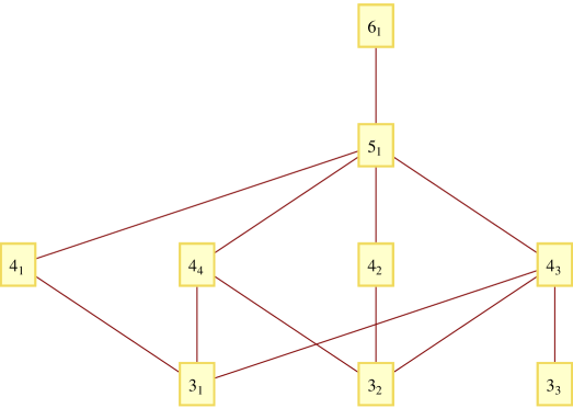
Figure 1: The family tree of texture zeros in $M_{\ell}$.

5 Numerical analysis

5.1 $\chi^{2}$-analysis

We perform a $\chi^{2}$-analysis of the different patterns of texture zeros. Our $\chi^{2}$-function has the usual form

$$\chi^{2}(x)\equiv\sum_{i}\left(\frac{P_{i}(x)-\overline{\mathcal{O}}_{i}}{\sigma_{i}}\right)^{2},$$ (21)

where the vector $x$ contains the model parameters, $P_{i}(x)$ is the model prediction for the observable $\mathcal{O}_{i}$ and $\overline{\mathcal{O}}_{i}$ is the central value for $\mathcal{O}_{i}$. The $\sigma_{i}$ are the errors of $\mathcal{O}_{i}$, where in case of asymmetric error distributions we use $\sigma_{i}^{\text{left}}$ and $\sigma_{i}^{\text{right}}$ for $P_{i}(x)\leq\overline{\mathcal{O}}_{i}$ and $P_{i}(x)>\overline{\mathcal{O}}_{i}$, respectively. In this paper we fit the lepton mass matrices with texture zeros to the eight observables

$$m_{e},\,m_{\mu},\,m_{\tau},\,\Delta m_{21}^{2},\,\Delta m_{31}^{2},\,\mathrm{sin}^{2}\theta_{12},\,\mathrm{sin}^{2}\theta_{23}\quad\text{and}\quad\mathrm{sin}^{2}\theta_{13}.$$

We do not fit the Dirac phase $\delta$. The central values and errors of the five neutrino oscillation parameters are taken from the global fit of oscillation data by Fogli et al. [4]. As central values of the charged-lepton masses we take the values from the Review of Particle Physics [51]. Since the experimental errors on the charged-lepton masses are so small that they can cause problems in the numerical $\chi^{2}$-analysis, we set them to one percent, i.e. $\sigma(m_{\ell})=0.01m_{\ell}$ for $\ell=e,\mu,\tau$. For details of the numerical implementation of the $\chi^{2}$-minimization, we refer the reader to appendix A.

Results of the $\chi^{2}$-analysis:

the only information we can obtain from the standard $\chi^{2}$-analysis is whether a given set of texture zeros in the mass matrices is excluded by the experimental data or not. We use the following criterion for a texture being compatible with the data:

We call a set of textures in the lepton mass matrices compatible with the data if at the minimum of $\chi^{2}$ the contribution of each observable to $\chi^{2}$ is at most $25$, i.e. the deviation of the observable from its experimental value is at most $5\sigma$. This implies that $\chi^{2}_{\text{min}}\leq 200$.

We find that according to this criterion about three quarters of the classes of texture zeros comprise viable textures. In the case of Dirac neutrinos all textures fulfilling the criterion have $\chi^{2}_{\text{min}}<10^{-4}$. In the case of Majorana neutrinos about 90 percent of the textures have $\chi^{2}_{\text{min}}<10^{-4}$, the remaining 10 percent have $\chi^{2}_{\text{min}}<30$ (normal spectrum) and $\chi^{2}_{\text{min}}<1$ (inverted spectrum).

Using the “family tree” of texture zeros discussed in section 4.3, we can identify the maximally restrictive textures among the compatible ones. This reduces the number of models to be investigated further to about 30 each for Dirac and Majorana neutrinos and for both neutrino mass spectra—see table 9. The compatible and maximally restrictive models are presented in tables 10 to 13. In only about a tenth of the compatible and maximally restrictive textures the charged-lepton mass matrix is diagonal, i.e. $M_{\ell}\sim 6_{1}^{(\ell)}$.

To summarize, by means of a $\chi^{2}$-analysis and the “family tree” of texture zeros we have arrived at the list of maximally restrictive texture zero models compatible with the experimental or observational data. In the following we will further investigate each model with regard to its predictivity.

Neutrino nature	Dirac		Majorana
Neutrino mass spectrum	normal	inverted	normal	inverted
Number of textures	$570$	$570$	$298$	$298$
Compatible with experiment	$430$	$429$	$215$	$229$
Compatible and maximally restrictive	$29$	$28$	$27$	$25$

Table 9: Results of the $\chi^{2}$-analysis.

5.2 Predictivity analysis

The $\chi^{2}$-analysis of the previous section only tells us which textures are compatible with the observations, but does not yield any statement on their predictive power. Therefore, we have developed a numerical method to estimate the predictive power of texture zeros in the lepton mass matrices. The main idea behind this method is to find an answer to the question:

Given matrices with a viable set of texture zeros and fixing the observables $\mathcal{O}_{j}$ $(j\neq i)$ to their experimentally observed values, how much can the remaining observable $\mathcal{O}_{i}$ at most deviate from its experimental or best-fit value?

In the following, we will outline our attempt to answer the above question for the observables we are interested in. Technical details of the numerical implementation of the method are presented in appendix A.

Consider a model with parameters $x$ making predictions $P_{i}(x)$ for the observables $\mathcal{O}_{i}$ with mean values $\overline{\mathcal{O}}_{i}$ and errors $\sigma_{i}$. For each observable $\mathcal{O}_{i}$, $\chi^{2}(x)$ has the contribution

$$\chi_{i}^{2}(x)\equiv\left(\frac{P_{i}(x)-\overline{\mathcal{O}}_{i}}{\sigma_{i}}\right)^{2}.$$ (22)

The contributions of all other observables to $\chi^{2}(x)$ are then given by

$$\widetilde{\chi}_{i}^{2}(x)\equiv\sum_{j\neq i}\left(\frac{P_{j}(x)-\overline{\mathcal{O}}_{j}}{\sigma_{j}}\right)^{2}=\chi^{2}(x)-\chi_{i}^{2}(x).$$ (23)

We define a measure for the maximal deviation of the observable $\mathcal{O}_{i}$ from its experimentally observed value as

$$\Delta(\mathcal{O}_{i})\equiv\max_{x\in B_{i}}\chi_{i}^{2}(x),$$ (24)

where $B_{i}$ is defined as

$$B_{i}\equiv\left\{\;x\;|\enspace\widetilde{\chi}_{i}^{2}(x)\leq\chi^{2}_{\text{min}}+\delta\chi^{2}\quad\text{and}\quad\chi_{j}^{2}(x)\leq 25\enspace\forall j\neq i\right\}$$ (25)

and $\chi^{2}_{\text{min}}$ is the minimum of $\chi^{2}(x)$ found in the $\chi^{2}$-analysis of section 5.1. The condition $x\in B_{i}$ fixes the other observables $\mathcal{O}_{j}$ $(j\neq i)$ to be close to their observed values $\overline{\mathcal{O}}_{j}$. The term $\delta\chi^{2}$ is added to $\chi^{2}_{\text{min}}$ in order to improve convergence of the numerical maximization of $\chi_{i}^{2}(x)$ in equation (24). In this paper, depending on the observable, we use either $\delta\chi^{2}=0$ or $\delta\chi^{2}=1$—see appendix A. The quantity $\Delta$ defined in equation (24) allows us to estimate the power of the studied set of texture zeros to predict $\mathcal{O}_{i}$. We will use this measure for a “predictivity analysis” of the five neutrino oscillation parameters and define:

A set of texture zeros can correctly predict the observable $\mathcal{O}_{i}$, where $\mathcal{O}_{i}$ is one of the observables $\Delta m_{21}^{2},\,\Delta m_{31}^{2},\,\mathrm{sin}^{2}\theta_{12},\,\mathrm{sin}^{2}\theta_{23},\,\mathrm{sin}^{2}\theta_{13}$, if

$$\Delta(\mathcal{O}_{i})\leq 100.$$ (26)

In other words, we stipulate that a set of texture zeros is capable to predict an observable $\mathcal{O}_{i}$ if its value can deviate from its central value $\overline{\mathcal{O}}_{i}$ by at most $10\sigma$, while the other observables $\mathcal{O}_{j}$ $(j\neq i)$ are kept close to their experimental or best-fit values.

For the charged-lepton masses we use a different predictivity measure. Namely, for each charged-lepton mass $m_{\ell}$ $(\ell=e,\mu,\tau)$ we compute its minimal and maximal values

$$m_{\ell}^{\mathrm{min}}\equiv\min_{x\in B_{m_{\ell}}}m_{\ell}(x)\quad\text{and}\quad m_{\ell}^{\mathrm{max}}\equiv\max_{x\in B_{m_{\ell}}}m_{\ell}(x)$$ (27)

and define:

A set of texture zeros can correctly predict the charged-lepton mass $m_{\ell}$ $(\ell=e,\mu,\tau)$ if

$$m_{\ell}^{\mathrm{min}}>\frac{1}{2}m_{\ell}^{\mathrm{exp}}\quad\text{and}\quad m_{\ell}^{\mathrm{max}}<2m_{\ell}^{\mathrm{exp}}.$$ (28)

Here $m_{\ell}^{\mathrm{exp}}$ denotes the mean experimental value of the charged-lepton mass $m_{\ell}$ taken from [51]. In words, we call a model predictive if it predicts that $m_{\ell}$ lies between $m_{\ell}^{\mathrm{exp}}/2$ and $2m_{\ell}^{\mathrm{exp}}$.

Finally, we also want to define a predictivity measure for those observables $\mathcal{O}$ which have not been measured up to now. In this case we compute the minimal and maximal value of $\mathcal{O}$ as

$$\mathcal{O}^{\mathrm{min}}\equiv\min_{x\in B}\mathcal{O}(x)\quad\text{and}\quad\mathcal{O}^{\mathrm{max}}\equiv\max_{x\in B}\mathcal{O}(x),$$ (29)

where the parameter set $B$ is defined as

$$B\equiv\left\{\;x\;|\enspace\chi^{2}(x)\leq\chi^{2}_{\text{min}}+\delta\chi^{2}\quad\text{and}\quad\chi_{j}^{2}(x)\leq 25\enspace\forall j\right\}.$$ (30)

Thus $B$ is similar to $B_{i}$ with $\widetilde{\chi}_{i}^{2}(x)$ replaced by the full $\chi^{2}$-function $\chi^{2}(x)$. In the numerical analysis performed for this paper we have computed $\mathcal{O}^{\mathrm{min}}$ and $\mathcal{O}^{\mathrm{max}}$ for the observables

$$m_{0},\,m_{\beta\beta},\,\delta,\,\rho\quad\text{and}\quad\sigma.$$ (31)

Here $m_{0}$ denotes the mass of the lightest neutrino, i.e. $m_{0}=m_{1}$ in the case of a normal and $m_{0}=m_{3}$ in the case of an inverted neutrino mass spectrum. The effective neutrino mass for neutrinoless double beta decay is given by

$$m_{\beta\beta}=\left|\sum_{k=1}^{3}(U_{\mathrm{PMNS}})_{ek}^{2}m_{k}\right|.$$ (32)

The Dirac CP-phase $\delta$ and the two Majorana phases $\rho$ and $\sigma$ are defined via the decomposition

$$U_{\text{PMNS}}=\exp(i\,\mathrm{diag}(\alpha,\,\beta,\,\gamma))\times\mathcal{U}(\theta_{12},\theta_{23},\theta_{13},\delta)\times\exp(i\,\mathrm{diag}(\rho,\,\sigma,\,0)),$$ (33)

where $\mathcal{U}$ stands for the standard parameterization of the mixing matrix [51]. The phases $\alpha$, $\beta$ and $\gamma$ are not accessible by experimental scrutiny. By definition, the range of the phases $\delta$, $\rho$ and $\sigma$ is $[0,2\pi)$. Since in all our numerical investigations we impose the constraint [51]

$$\sum_{k=1}^{3}m_{k}<1\,\text{eV}$$ (34)

on the absolute neutrino mass scale, $m_{0}$ and $m_{\beta\beta}$ can assume values between zero and about $1/3~{}\text{eV}$. Given these bounds, we may define:

A set of textures zeros can predict one of the observables $m_{0}$, $m_{\beta\beta}$, $\delta$, $\rho$, $\sigma$ if

$$\frac{\mathcal{O}^{\mathrm{max}}-\mathcal{O}^{\mathrm{min}}}{\mathrm{range}(\mathcal{O})}\leq 0.2.$$ (35)

Here $\mathrm{range}(m_{0})=\mathrm{range}(m_{\beta\beta})=1/3~{}\text{eV}$ and $\mathrm{range}(\delta)=\mathrm{range}(\rho)=\mathrm{range}(\sigma)=2\pi$.

Results of the predictivity analysis:

We have performed the analysis explained above for all viable and maximally restrictive texture-zero models. The results of this paper, i.e. the viable and maximally restrictive textures and their predictions, are presented in four tables:

1. table 10: Dirac neutrinos with normal ordering of the neutrino masses,

2. table 11: Dirac neutrinos with inverted ordering of the neutrino masses,

3. table 12: Majorana neutrinos with normal ordering of the neutrino masses,

4. table 13: Majorana neutrinos with inverted ordering of the neutrino masses.

In these tables, $n$ denotes the number of real parameters of the model after removing as many phases as possible from the elements of the mass matrices by means of weak-basis transformations.

The results of the predictivity analysis may be summarized as follows.

• According to the criterion of equation (28), none of the investigated textures can predict any of the charged-lepton masses. Also relaxing the condition (28) for $m_{e}$ to $m_{e}^{\mathrm{min}}>0.1~{}\text{MeV},m_{e}^{\mathrm{max}}<5~{}\text{MeV}$ does not change this result.

• Only one set of texture zeros discussed in this paper fulfills the requirement of equation (26). Namely, for the texture $(M_{\ell},M_{L})\sim(6_{1}^{(\ell)},2_{1}^{(\nu_{L})})$ with an inverted neutrino mass spectrum one has $\Delta(\mathrm{sin}^{2}\theta_{23})=53.8<100$. However, tightening the criterion of equation (26) to $\Delta(\mathcal{O}_{i})\leq 25$, i.e. to $5\sigma$, there is no texture which can predict any of the charged-lepton masses or the neutrino oscillation parameters.

• Most of the investigated textures can predict the smallest neutrino mass $m_{0}$. In the case of Dirac neutrinos, all but two of the maximally restrictive viable textures have $\mathrm{rank}(M_{D})=2$ and thus $m_{0}=0$.

• For all but one of the maximally predictive and compatible textures for Dirac neutrinos we find $\delta^{\mathrm{min}}\approx 0$ and $\delta^{\mathrm{max}}\approx 2\pi$. The only exception is the texture $(M_{\ell},M_{D})\sim(6_{1}^{(\ell)},4_{5}^{(\nu_{D})})$ with a normal neutrino mass spectrum, where one finds $\delta^{\mathrm{min}}=0$ and $\delta^{\mathrm{max}}=\pi$ within the numerical accuracy. In fact, through a weak-basis transformation (10a) with $V_{L}$, $V_{R}^{(\ell)}$ and $V_{R}^{(\nu)}$ being diagonal phase matrices, in this case $M_{\ell}$ and $M_{D}$ can be made real simultaneously, which implies $\delta\in\{0,\pi\}$. Therefore, this texture does not admit CP violation in neutrino oscillations.

• Many of the textures for the Majorana neutrino case are predictive with respect to the Dirac phase $\delta$. In contrast to the case of Dirac neutrinos, here also $\delta\neq 0,\pi$ is possible.

• None of the textures for Majorana neutrinos can predict any of the Majorana phases $\rho$ and $\sigma$ according to the condition of equation (35).

• Almost all maximally restrictive and compatible sets of textures in $(M_{\ell},M_{L})$ predict $m_{\beta\beta}$.

• The effective mass $m_{\beta\beta}$ can be big (larger than 0.1 eV) or small for normal ordering of the neutrino mass spectrum, however, for the inverted spectrum we always find $m_{\beta\beta}<0.1$ eV.

• There are a few instances where $M_{D}$ or $M_{L}$ are diagonal and lepton mixing comes purely from $M_{\ell}$. Since we deal with maximally restrictive textures, in all of these instances we trivially have $m_{0}=0$.

Thus, the most interesting results of the predictivity analysis are the minima and maxima of $m_{0}$, $\delta$ and $m_{\beta\beta}$, which we also show in tables 10 to 13. As for $\cos\delta$ and Majorana textures with diagonal $M_{\ell}$—see the last three lines in tables 12 and 13, we have checked that our results agree with those of [18].

A note of caution on the interpretation of the results:

The presented method for estimating the predictivity of a texture-zero model is based on maximal deviations from the observed value, see the definition of $\Delta$ in equation (24), and maximal and minimal values of observables, see equations (27) and (29). Therefore, some of the models may still possess predictive power which can, however, not be measured by these quantities. For example, the texture $(M_{\ell},M_{D})\sim(6_{1}^{(\ell)},4_{5}^{(\nu_{D})})$ allows $\delta$ to assume only the values zero and $\pi$, i.e. we would call this model “predictive” with respect to $\delta$. But in this case our analysis does not detect predictive power because equation (35) then reads

$$\frac{\delta^{\mathrm{max}}-\delta^{\mathrm{min}}}{\mathrm{range}(\delta)}=\frac{\pi-0}{2\pi}=\frac{1}{2}>0.2.$$ (36)

$(M_{\ell},M_{D})$	$n$	$m_{0}^{\mathrm{min}}\,\text{[eV]}$	$m_{0}^{\mathrm{max}}\,\text{[eV]}$	texture predicts
$3_{2}-7_{1}$	$9$	$0.00\times 10^{0}$	$0.00\times 10^{0}$	$m_{0}$
$3_{2}-7_{3}$	$9$	$0.00\times 10^{0}$	$0.00\times 10^{0}$	$m_{0}$
$4_{1}-6_{1}$	$9$	$0.00\times 10^{0}$	$0.00\times 10^{0}$	$m_{0}$
$4_{1}-6_{3}$	$9$	$0.00\times 10^{0}$	$0.00\times 10^{0}$	$m_{0}$
$4_{1}-6_{4}$	$9$	$0.00\times 10^{0}$	$0.00\times 10^{0}$	$m_{0}$
$4_{1}-6_{5}$	$9$	$0.00\times 10^{0}$	$0.00\times 10^{0}$	$m_{0}$
$4_{1}-6_{6}$	$9$	$0.00\times 10^{0}$	$0.00\times 10^{0}$	$m_{0}$
$4_{2}-6_{1}$	$9$	$0.00\times 10^{0}$	$0.00\times 10^{0}$	$m_{0}$
$4_{2}-6_{2}$	$9$	$0.00\times 10^{0}$	$0.00\times 10^{0}$	$m_{0}$
$4_{2}-6_{3}$	$9$	$0.00\times 10^{0}$	$0.00\times 10^{0}$	$m_{0}$
$4_{2}-6_{7}$	$9$	$0.00\times 10^{0}$	$0.00\times 10^{0}$	$m_{0}$
$4_{2}-6_{8}$	$9$	$0.00\times 10^{0}$	$0.00\times 10^{0}$	$m_{0}$
$4_{3}-6_{1}$	$9$	$0.00\times 10^{0}$	$0.00\times 10^{0}$	$m_{0}$
$4_{3}-6_{2}$	$9$	$0.00\times 10^{0}$	$0.00\times 10^{0}$	$m_{0}$
$4_{3}-6_{3}$	$9$	$0.00\times 10^{0}$	$0.00\times 10^{0}$	$m_{0}$
$4_{3}-6_{4}$	$9$	$0.00\times 10^{0}$	$0.00\times 10^{0}$	$m_{0}$
$4_{3}-6_{5}$	$9$	$0.00\times 10^{0}$	$0.00\times 10^{0}$	$m_{0}$
$4_{3}-6_{6}$	$9$	$0.00\times 10^{0}$	$0.00\times 10^{0}$	$m_{0}$
$4_{3}-6_{7}$	$9$	$0.00\times 10^{0}$	$0.00\times 10^{0}$	$m_{0}$
$4_{3}-6_{8}$	$9$	$0.00\times 10^{0}$	$0.00\times 10^{0}$	$m_{0}$
$4_{3}-6_{9}$	$9$	$0.00\times 10^{0}$	$0.00\times 10^{0}$	$m_{0}$
$5_{1}-5_{1}$	$9$	$0.00\times 10^{0}$	$0.00\times 10^{0}$	$m_{0}$
$5_{1}-5_{4}$	$9$	$0.00\times 10^{0}$	$0.00\times 10^{0}$	$m_{0}$
$5_{1}-5_{5}$	$9$	$0.00\times 10^{0}$	$0.00\times 10^{0}$	$m_{0}$
$5_{1}-5_{6}$	$9$	$0.00\times 10^{0}$	$0.00\times 10^{0}$	$m_{0}$
$5_{1}-5_{8}$	$9$	$0.00\times 10^{0}$	$0.00\times 10^{0}$	$m_{0}$
$6_{1}-3_{12}$	$10$	$1.69\times 10^{-2}$	$3.32\times 10^{-1}$	—
$6_{1}-4_{1}$	$9$	$0.00\times 10^{0}$	$0.00\times 10^{0}$	$m_{0}$
$6_{1}-4_{5}$	$8$	$1.15\times 10^{-2}$	$1.65\times 10^{-2}$	$m_{0}$

Table 10: The maximally restrictive and compatible classes of texture zeros in $(M_{\ell},M_{D})$. The number of physical parameters of the texture is denoted by $n$. For all textures in this table $\chi^{2}_{\mathrm{min}}<10^{-4}$. For the Dirac phase $\delta$ one finds $\delta^{\mathrm{min}}\approx 0$ and $\delta^{\mathrm{max}}\approx 2\pi$ for all textures except $6_{1}-4_{5}$, where $\delta=0$ or $\pi$. Part 1: normal neutrino mass spectrum.

$(M_{\ell},M_{D})$	$n$	$m_{0}^{\mathrm{min}}\,\text{[eV]}$	$m_{0}^{\mathrm{max}}\,\text{[eV]}$	texture predicts
$3_{2}-7_{1}$	$9$	$0.00\times 10^{0}$	$0.00\times 10^{0}$	$m_{0}$
$3_{2}-7_{3}$	$9$	$0.00\times 10^{0}$	$0.00\times 10^{0}$	$m_{0}$
$4_{1}-6_{1}$	$9$	$0.00\times 10^{0}$	$0.00\times 10^{0}$	$m_{0}$
$4_{1}-6_{3}$	$9$	$0.00\times 10^{0}$	$0.00\times 10^{0}$	$m_{0}$
$4_{1}-6_{4}$	$9$	$0.00\times 10^{0}$	$0.00\times 10^{0}$	$m_{0}$
$4_{1}-6_{5}$	$9$	$0.00\times 10^{0}$	$0.00\times 10^{0}$	$m_{0}$
$4_{1}-6_{6}$	$9$	$0.00\times 10^{0}$	$0.00\times 10^{0}$	$m_{0}$
$4_{2}-6_{1}$	$9$	$0.00\times 10^{0}$	$0.00\times 10^{0}$	$m_{0}$
$4_{2}-6_{2}$	$9$	$0.00\times 10^{0}$	$0.00\times 10^{0}$	$m_{0}$
$4_{2}-6_{3}$	$9$	$0.00\times 10^{0}$	$0.00\times 10^{0}$	$m_{0}$
$4_{2}-6_{7}$	$9$	$0.00\times 10^{0}$	$0.00\times 10^{0}$	$m_{0}$
$4_{2}-6_{8}$	$9$	$0.00\times 10^{0}$	$0.00\times 10^{0}$	$m_{0}$
$4_{3}-6_{1}$	$9$	$0.00\times 10^{0}$	$0.00\times 10^{0}$	$m_{0}$
$4_{3}-6_{2}$	$9$	$0.00\times 10^{0}$	$0.00\times 10^{0}$	$m_{0}$
$4_{3}-6_{3}$	$9$	$0.00\times 10^{0}$	$0.00\times 10^{0}$	$m_{0}$
$4_{3}-6_{4}$	$9$	$0.00\times 10^{0}$	$0.00\times 10^{0}$	$m_{0}$
$4_{3}-6_{5}$	$9$	$0.00\times 10^{0}$	$0.00\times 10^{0}$	$m_{0}$
$4_{3}-6_{6}$	$9$	$0.00\times 10^{0}$	$0.00\times 10^{0}$	$m_{0}$
$4_{3}-6_{7}$	$9$	$0.00\times 10^{0}$	$0.00\times 10^{0}$	$m_{0}$
$4_{3}-6_{8}$	$9$	$0.00\times 10^{0}$	$0.00\times 10^{0}$	$m_{0}$
$4_{3}-6_{9}$	$9$	$0.00\times 10^{0}$	$0.00\times 10^{0}$	$m_{0}$
$5_{1}-5_{1}$	$9$	$0.00\times 10^{0}$	$0.00\times 10^{0}$	$m_{0}$
$5_{1}-5_{4}$	$9$	$0.00\times 10^{0}$	$0.00\times 10^{0}$	$m_{0}$
$5_{1}-5_{5}$	$9$	$0.00\times 10^{0}$	$0.00\times 10^{0}$	$m_{0}$
$5_{1}-5_{6}$	$9$	$0.00\times 10^{0}$	$0.00\times 10^{0}$	$m_{0}$
$5_{1}-5_{8}$	$9$	$0.00\times 10^{0}$	$0.00\times 10^{0}$	$m_{0}$
$6_{1}-3_{12}$	$10$	$<10^{-3}$	$3.31\times 10^{-1}$	—
$6_{1}-4_{1}$	$9$	$0.00\times 10^{0}$	$0.00\times 10^{0}$	$m_{0}$

Table 11: The maximally restrictive and compatible classes of texture zeros in $(M_{\ell},M_{D})$. The number of physical parameters of the texture is denoted by $n$. For all textures in this table $\chi^{2}_{\mathrm{min}}<10^{-4}$, $\delta^{\mathrm{min}}\approx 0$ and $\delta^{\mathrm{max}}\approx 2\pi$. Part 2: inverted neutrino mass spectrum.

$(M_{\ell},M_{L})$	$n$	$\chi^{2}_{\mathrm{min}}$	$m_{0}^{\mathrm{min}}\,\text{[eV]}$	$m_{0}^{\mathrm{max}}\,\text{[eV]}$	$\delta^{\mathrm{min}}$	$\delta^{\mathrm{max}}$	$m_{\beta\beta}^{\mathrm{min}}\,\text{[eV]}$	$m_{\beta\beta}^{\mathrm{max}}\,\text{[eV]}$	texture predicts
$3_{2}-4_{7}$	$10$	$<10^{-4}$	$0.00\times 10^{0}$	$0.00\times 10^{0}$	$<10^{-2}$	$6.27\times 10^{0}$	$1.34\times 10^{-3}$	$3.86\times 10^{-3}$	$m_{0}$, $m_{\beta\beta}$
$3_{2}-4_{9}$	$10$	$<10^{-4}$	$0.00\times 10^{0}$	$0.00\times 10^{0}$	$<10^{-2}$	$6.28\times 10^{0}$	$1.34\times 10^{-3}$	$3.86\times 10^{-3}$	$m_{0}$, $m_{\beta\beta}$
$4_{1}-3_{3}$	$10$	$<10^{-4}$	$1.17\times 10^{-3}$	$3.32\times 10^{-1}$	$<10^{-2}$	$6.28\times 10^{0}$	$<10^{-3}$	$2.14\times 10^{-1}$	—
$4_{1}-3_{15}$	$10$	$2.63\times 10^{-2}$	$4.49\times 10^{-2}$	$3.32\times 10^{-1}$	$2.92\times 10^{0}$	$3.37\times 10^{0}$	$1.45\times 10^{-2}$	$1.34\times 10^{-1}$	$\delta$
$4_{1}-4_{1}$	$8$	$2.99\times 10^{1}$	$0.00\times 10^{0}$	$0.00\times 10^{0}$	$3.07\times 10^{0}$	$3.21\times 10^{0}$	$1.57\times 10^{-3}$	$1.69\times 10^{-3}$	$m_{0}$, $\delta$, $m_{\beta\beta}$
$4_{1}-4_{4}$	$8$	$2.80\times 10^{1}$	$0.00\times 10^{0}$	$0.00\times 10^{0}$	$3.07\times 10^{0}$	$3.21\times 10^{0}$	$1.56\times 10^{-3}$	$1.69\times 10^{-3}$	$m_{0}$, $\delta$, $m_{\beta\beta}$
$4_{2}-3_{2}$	$10$	$<10^{-4}$	$0.00\times 10^{0}$	$0.00\times 10^{0}$	$<10^{-2}$	$6.27\times 10^{0}$	$1.34\times 10^{-3}$	$3.86\times 10^{-3}$	$m_{0}$, $m_{\beta\beta}$
$4_{2}-3_{3}$	$10$	$<10^{-4}$	$<10^{-3}$	$9.24\times 10^{-2}$	$<10^{-2}$	$6.27\times 10^{0}$	$<10^{-3}$	$6.09\times 10^{-2}$	$m_{\beta\beta}$
$4_{2}-3_{6}$	$10$	$<10^{-4}$	$<10^{-3}$	$9.28\times 10^{-2}$	$<10^{-2}$	$6.27\times 10^{0}$	$1.19\times 10^{-3}$	$6.10\times 10^{-2}$	$m_{\beta\beta}$
$4_{2}-3_{8}$	$10$	$<10^{-4}$	$3.23\times 10^{-3}$	$6.10\times 10^{-3}$	$<10^{-2}$	$6.28\times 10^{0}$	$<10^{-3}$	$2.10\times 10^{-3}$	$m_{0}$, $m_{\beta\beta}$
$4_{2}-3_{10}$	$10$	$<10^{-4}$	$0.00\times 10^{0}$	$0.00\times 10^{0}$	$<10^{-2}$	$6.28\times 10^{0}$	$1.34\times 10^{-3}$	$3.86\times 10^{-3}$	$m_{0}$, $m_{\beta\beta}$
$4_{2}-3_{11}$	$10$	$<10^{-4}$	$0.00\times 10^{0}$	$0.00\times 10^{0}$	$<10^{-2}$	$6.28\times 10^{0}$	$1.34\times 10^{-3}$	$3.86\times 10^{-3}$	$m_{0}$, $m_{\beta\beta}$
$4_{2}-3_{12}$	$10$	$<10^{-4}$	$1.71\times 10^{-3}$	$4.44\times 10^{-3}$	$<10^{-2}$	$6.28\times 10^{0}$	$1.16\times 10^{-3}$	$2.71\times 10^{-3}$	$m_{0}$, $m_{\beta\beta}$
$4_{2}-3_{14}$	$10$	$<10^{-4}$	$1.71\times 10^{-3}$	$4.44\times 10^{-3}$	$<10^{-2}$	$6.28\times 10^{0}$	$1.16\times 10^{-3}$	$2.71\times 10^{-3}$	$m_{0}$, $m_{\beta\beta}$
$4_{2}-3_{16}$	$10$	$<10^{-4}$	$0.00\times 10^{0}$	$0.00\times 10^{0}$	$<10^{-2}$	$6.28\times 10^{0}$	$1.34\times 10^{-3}$	$3.86\times 10^{-3}$	$m_{0}$, $m_{\beta\beta}$
$4_{3}-3_{4}$	$10$	$<10^{-4}$	$1.17\times 10^{-3}$	$3.32\times 10^{-1}$	$<10^{-2}$	$6.28\times 10^{0}$	$<10^{-3}$	$2.14\times 10^{-1}$	—
$4_{3}-3_{9}$	$10$	$<10^{-4}$	$1.17\times 10^{-3}$	$3.32\times 10^{-1}$	$<10^{-2}$	$6.28\times 10^{0}$	$<10^{-3}$	$2.14\times 10^{-1}$	—
$4_{3}-3_{14}$	$10$	$2.63\times 10^{-2}$	$4.49\times 10^{-2}$	$3.32\times 10^{-1}$	$2.92\times 10^{0}$	$3.37\times 10^{0}$	$1.45\times 10^{-2}$	$1.34\times 10^{-1}$	$\delta$
$4_{3}-3_{18}$	$10$	$2.63\times 10^{-2}$	$4.49\times 10^{-2}$	$3.32\times 10^{-1}$	$2.92\times 10^{0}$	$3.37\times 10^{0}$	$1.45\times 10^{-2}$	$1.34\times 10^{-1}$	$\delta$
$4_{3}-4_{2}$	$8$	$2.99\times 10^{1}$	$0.00\times 10^{0}$	$0.00\times 10^{0}$	$3.07\times 10^{0}$	$3.21\times 10^{0}$	$1.57\times 10^{-3}$	$1.69\times 10^{-3}$	$m_{0}$, $\delta$, $m_{\beta\beta}$
$4_{3}-4_{3}$	$8$	$2.80\times 10^{1}$	$0.00\times 10^{0}$	$0.00\times 10^{0}$	$3.07\times 10^{0}$	$3.21\times 10^{0}$	$1.56\times 10^{-3}$	$1.69\times 10^{-3}$	$m_{0}$, $\delta$, $m_{\beta\beta}$
$4_{3}-4_{4}$	$8$	$2.99\times 10^{1}$	$0.00\times 10^{0}$	$0.00\times 10^{0}$	$3.07\times 10^{0}$	$3.21\times 10^{0}$	$1.57\times 10^{-3}$	$1.69\times 10^{-3}$	$m_{0}$, $\delta$, $m_{\beta\beta}$
$4_{3}-4_{5}$	$8$	$2.80\times 10^{1}$	$0.00\times 10^{0}$	$0.00\times 10^{0}$	$3.07\times 10^{0}$	$3.21\times 10^{0}$	$1.56\times 10^{-3}$	$1.69\times 10^{-3}$	$m_{0}$, $\delta$, $m_{\beta\beta}$
$5_{1}-3_{1}$	$8$	$3.87\times 10^{0}$	$2.76\times 10^{-2}$	$2.79\times 10^{-2}$	$2.11\times 10^{0}$	$4.18\times 10^{0}$	$2.60\times 10^{-2}$	$2.78\times 10^{-2}$	$m_{0}$, $m_{\beta\beta}$
$6_{1}-2_{1}$	$8$	$2.25\times 10^{1}$	$1.52\times 10^{-1}$	$3.32\times 10^{-1}$	$<10^{-2}$	$6.28\times 10^{0}$	$1.44\times 10^{-1}$	$3.29\times 10^{-1}$	—
$6_{1}-2_{4}$	$8$	$<10^{-4}$	$4.00\times 10^{-3}$	$4.21\times 10^{-2}$	$1.32\times 10^{0}$	$4.96\times 10^{0}$	$0.00\times 10^{0}$	$4.29\times 10^{-2}$	$m_{0}$, $m_{\beta\beta}$
$6_{1}-2_{6}$	$8$	$<10^{-4}$	$3.52\times 10^{-2}$	$3.91\times 10^{-2}$	$1.64\times 10^{0}$	$4.64\times 10^{0}$	$3.58\times 10^{-2}$	$3.97\times 10^{-2}$	$m_{0}$, $m_{\beta\beta}$

Table 12: The maximally restrictive and compatible classes of texture zeros in $(M_{\ell},M_{L})$. The number of physical parameters of the texture is denoted by $n$. Part 1: normal neutrino mass spectrum.

$(M_{\ell},M_{L})$	$n$	$\chi^{2}_{\mathrm{min}}$	$m_{0}^{\mathrm{min}}\,\text{[eV]}$	$m_{0}^{\mathrm{max}}\,\text{[eV]}$	$\delta^{\mathrm{min}}$	$\delta^{\mathrm{max}}$	$m_{\beta\beta}^{\mathrm{min}}\,\text{[eV]}$	$m_{\beta\beta}^{\mathrm{max}}\,\text{[eV]}$	texture predicts
$3_{2}-4_{7}$	$10$	$<10^{-4}$	$0.00\times 10^{0}$	$0.00\times 10^{0}$	$<10^{-2}$	$6.28\times 10^{0}$	$1.79\times 10^{-2}$	$4.88\times 10^{-2}$	$m_{0}$, $m_{\beta\beta}$
$3_{2}-4_{9}$	$10$	$<10^{-4}$	$0.00\times 10^{0}$	$0.00\times 10^{0}$	$<10^{-2}$	$6.27\times 10^{0}$	$1.79\times 10^{-2}$	$4.88\times 10^{-2}$	$m_{0}$, $m_{\beta\beta}$
$4_{1}-4_{1}$	$8$	$2.43\times 10^{-3}$	$0.00\times 10^{0}$	$0.00\times 10^{0}$	$2.87\times 10^{0}$	$3.41\times 10^{0}$	$1.80\times 10^{-2}$	$1.87\times 10^{-2}$	$m_{0}$, $\delta$, $m_{\beta\beta}$
$4_{1}-4_{2}$	$8$	$1.41\times 10^{-1}$	$0.00\times 10^{0}$	$0.00\times 10^{0}$	$2.97\times 10^{0}$	$3.31\times 10^{0}$	$1.76\times 10^{-2}$	$1.82\times 10^{-2}$	$m_{0}$, $\delta$, $m_{\beta\beta}$
$4_{1}-4_{4}$	$8$	$2.75\times 10^{-2}$	$0.00\times 10^{0}$	$0.00\times 10^{0}$	$2.92\times 10^{0}$	$3.37\times 10^{0}$	$1.79\times 10^{-2}$	$1.85\times 10^{-2}$	$m_{0}$, $\delta$, $m_{\beta\beta}$
$4_{2}-3_{11}$	$10$	$<10^{-4}$	$0.00\times 10^{0}$	$0.00\times 10^{0}$	$<10^{-2}$	$6.28\times 10^{0}$	$1.79\times 10^{-2}$	$4.88\times 10^{-2}$	$m_{0}$, $m_{\beta\beta}$
$4_{2}-3_{14}$	$10$	$<10^{-4}$	$1.73\times 10^{-3}$	$4.26\times 10^{-3}$	$<10^{-2}$	$6.27\times 10^{0}$	$1.78\times 10^{-2}$	$4.89\times 10^{-2}$	$m_{0}$, $m_{\beta\beta}$
$4_{2}-3_{16}$	$10$	$<10^{-4}$	$0.00\times 10^{0}$	$0.00\times 10^{0}$	$<10^{-2}$	$6.27\times 10^{0}$	$1.79\times 10^{-2}$	$4.88\times 10^{-2}$	$m_{0}$, $m_{\beta\beta}$
$4_{2}-3_{17}$	$10$	$<10^{-4}$	$1.73\times 10^{-3}$	$4.26\times 10^{-3}$	$<10^{-2}$	$6.27\times 10^{0}$	$1.78\times 10^{-2}$	$4.89\times 10^{-2}$	$m_{0}$, $m_{\beta\beta}$
$4_{3}-4_{1}$	$8$	$1.41\times 10^{-1}$	$0.00\times 10^{0}$	$0.00\times 10^{0}$	$2.97\times 10^{0}$	$3.31\times 10^{0}$	$1.76\times 10^{-2}$	$1.82\times 10^{-2}$	$m_{0}$, $\delta$, $m_{\beta\beta}$
$4_{3}-4_{2}$	$8$	$2.43\times 10^{-3}$	$0.00\times 10^{0}$	$0.00\times 10^{0}$	$2.87\times 10^{0}$	$3.41\times 10^{0}$	$1.80\times 10^{-2}$	$1.87\times 10^{-2}$	$m_{0}$, $\delta$, $m_{\beta\beta}$
$4_{3}-4_{3}$	$8$	$2.75\times 10^{-2}$	$0.00\times 10^{0}$	$0.00\times 10^{0}$	$2.92\times 10^{0}$	$3.37\times 10^{0}$	$1.79\times 10^{-2}$	$1.85\times 10^{-2}$	$m_{0}$, $\delta$, $m_{\beta\beta}$
$4_{3}-4_{4}$	$8$	$2.43\times 10^{-3}$	$0.00\times 10^{0}$	$0.00\times 10^{0}$	$2.87\times 10^{0}$	$3.41\times 10^{0}$	$1.80\times 10^{-2}$	$1.87\times 10^{-2}$	$m_{0}$, $\delta$, $m_{\beta\beta}$
$4_{3}-4_{5}$	$8$	$2.75\times 10^{-2}$	$0.00\times 10^{0}$	$0.00\times 10^{0}$	$2.92\times 10^{0}$	$3.37\times 10^{0}$	$1.79\times 10^{-2}$	$1.85\times 10^{-2}$	$m_{0}$, $\delta$, $m_{\beta\beta}$
$4_{3}-4_{6}$	$8$	$1.41\times 10^{-1}$	$0.00\times 10^{0}$	$0.00\times 10^{0}$	$2.97\times 10^{0}$	$3.31\times 10^{0}$	$1.76\times 10^{-2}$	$1.82\times 10^{-2}$	$m_{0}$, $\delta$, $m_{\beta\beta}$
$5_{1}-3_{1}$	$8$	$<10^{-4}$	$<10^{-3}$	$<10^{-3}$	$2.83\times 10^{0}$	$3.46\times 10^{0}$	$1.81\times 10^{-2}$	$1.89\times 10^{-2}$	$m_{0}$, $\delta$, $m_{\beta\beta}$
$5_{1}-3_{2}$	$8$	$1.80\times 10^{-1}$	$0.00\times 10^{0}$	$0.00\times 10^{0}$	$2.98\times 10^{0}$	$3.31\times 10^{0}$	$1.75\times 10^{-2}$	$1.81\times 10^{-2}$	$m_{0}$, $\delta$, $m_{\beta\beta}$
$5_{1}-3_{3}$	$8$	$<10^{-4}$	$1.05\times 10^{-3}$	$1.14\times 10^{-3}$	$2.58\times 10^{0}$	$3.71\times 10^{0}$	$1.95\times 10^{-2}$	$2.04\times 10^{-2}$	$m_{0}$, $\delta$, $m_{\beta\beta}$
$5_{1}-3_{6}$	$8$	$5.64\times 10^{-1}$	$<10^{-3}$	$<10^{-3}$	$3.01\times 10^{0}$	$3.27\times 10^{0}$	$1.70\times 10^{-2}$	$1.76\times 10^{-2}$	$m_{0}$, $\delta$, $m_{\beta\beta}$
$5_{1}-3_{7}$	$8$	$<10^{-4}$	$1.05\times 10^{-3}$	$1.14\times 10^{-3}$	$2.58\times 10^{0}$	$3.71\times 10^{0}$	$1.95\times 10^{-2}$	$2.04\times 10^{-2}$	$m_{0}$, $\delta$, $m_{\beta\beta}$
$5_{1}-3_{8}$	$8$	$5.64\times 10^{-1}$	$<10^{-3}$	$<10^{-3}$	$3.01\times 10^{0}$	$3.27\times 10^{0}$	$1.70\times 10^{-2}$	$1.76\times 10^{-2}$	$m_{0}$, $\delta$, $m_{\beta\beta}$
$5_{1}-3_{10}$	$8$	$1.80\times 10^{-1}$	$0.00\times 10^{0}$	$0.00\times 10^{0}$	$2.98\times 10^{0}$	$3.31\times 10^{0}$	$1.75\times 10^{-2}$	$1.81\times 10^{-2}$	$m_{0}$, $\delta$, $m_{\beta\beta}$
$6_{1}-2_{1}$	$8$	$<10^{-4}$	$3.31\times 10^{-2}$	$4.02\times 10^{-2}$	$8.65\times 10^{-1}$	$5.42\times 10^{0}$	$3.26\times 10^{-2}$	$3.99\times 10^{-2}$	$\mathrm{sin}^{2}\theta_{23}$, $m_{0}$, $m_{\beta\beta}$
$6_{1}-2_{4}$	$8$	$<10^{-4}$	$4.10\times 10^{-2}$	$4.72\times 10^{-2}$	$1.55\times 10^{0}$	$4.73\times 10^{0}$	$6.37\times 10^{-2}$	$6.80\times 10^{-2}$	$m_{0}$, $m_{\beta\beta}$
$6_{1}-2_{6}$	$8$	$<10^{-4}$	$3.80\times 10^{-2}$	$4.39\times 10^{-2}$	$1.57\times 10^{0}$	$4.71\times 10^{0}$	$6.19\times 10^{-2}$	$6.58\times 10^{-2}$	$m_{0}$, $m_{\beta\beta}$

Table 13: The maximally restrictive and compatible classes of texture zeros in $(M_{\ell},M_{L})$. The number of physical parameters of the texture is denoted by $n$. Part 2: inverted neutrino mass spectrum.

6 Conclusions

In this paper we have performed a thorough analysis of texture zeros in lepton mass matrices for both Dirac and Majorana neutrinos. It is instructive to summarize our basic assumptions. Firstly, we assume that there are three families of leptons, which means that the charged-lepton mass matrix $M_{\ell}$, the Dirac neutrino mass matrix $M_{D}$ and the Majorana neutrino mass matrix $M_{L}$ are all $3\times 3$ matrices. Secondly, the tree-level mass matrices which contain the texture zeros should be compatible with our knowledge about the lepton masses and the lepton mixing matrix, which leads us to the requirements $\text{rank}(M_{\ell})=3$ and $\text{rank}(M_{D})\,\mbox{or}\ \text{rank}(M_{L})\geq 2$ and excludes some textures in $M_{L}$ with degenerate neutrino masses. Thirdly, the gauge-multiplet structure of the lepton fields is the same as in the Standard Model, i.e. left-handed doublets and right-handed singlets. This last assumption fixes the allowed forms of weak-basis transformations; for instance, in the case of Dirac neutrinos we are allowed to perform independent weak-basis transformations on the right-handed charged-lepton fields and the right-handed neutrino fields.

One of the main points of this paper is that we admit all possible combinations of texture zeros in the pairs of mass matrices $(M_{\ell},M_{D})$ and $(M_{\ell},M_{L})$. In particular, we allow for non-diagonal $M_{\ell}$. Since there is a huge number of such combinations even after taking into account the second assumption above, we had to address the problem of equivalent texture zeros in the pairs of mass matrices, i.e. textures which are related through weak-basis transformations with permutation matrices (weak-basis permutations). We have found 570 inequivalent classes of texture zeros in the Dirac case and 298 classes in the Majorana case; for both cases about 75% of the classes are compatible with the data. However, if we consider only classes which are maximally restrictive—cf. section 4.3, we are down to about 30 classes of texture zeros for each of the four categories defined by Dirac/Majorana nature and normal/inverted ordering of the neutrino mass spectrum—see table 9.

We have also attempted to identify the predictive classes of texture zeros by defining numerical measures of predictivity in section 5.2. However, applying these measures to the eight experimentally known observables, namely charged-lepton masses, neutrino mass-squared differences and mixing angles, it turned out that, for all but one of the models, none of these eight observables can be predicted by using the values of the other seven observables as input. On the other hand, using the values of all eight known observables it is possible to predict in almost all viable and maximally restrictive classes of texture zeros the smallest neutrino mass $m_{0}$ and thus the absolute neutrino mass scale. However, even this has a rather trivial explanation: most of these classes of texture zeros predict $m_{0}=0$, but in these cases the neutrino mass matrix has always rank two. The small rank of most neutrino mass matrices is simply the consequence that we consider maximally restrictive classes. The main results of this paper are summarized in tables 10 to 13.

In summary, pure texture zero models are astonishingly weak in their predictions. This also holds for the hitherto neglected scenarios where $M_{\ell}$ is non-diagonal. Of course, it could be that texture zero models which we have excluded in this work because they fail at the tree level become compatible with the data and are predictive when radiative corrections are taken into account. Apart from this loop hole, we rather draw the conclusion that predictive mass matrices need also relations among the non-zero matrix elements.

Acknowledgments:

This work is supported by the Austrian Science Fund (FWF), Project No. P 24161-N16. P.O.L. thanks Helmut Moser for his tireless servicing of our research group’s computer cluster on which the computations for this work were performed.

Appendix A Details on the numerical analysis

All numerical methods used in this work are based on minimization or maximization of functions of real parameters $x\in\mathbbm{R}^{n}$. Since maximization of a real-valued function $f(x)$ can be achieved by minimizing $-f(x)$, we only need a minimization algorithm. Our algorithm of choice is the Nelder-Mead downhill simplex algorithm [52], which we implemented in the programming language C [53]. To increase the quality of the minima, the algorithm was started repeatedly with different “start simplices”. In order to further improve the quality of the minima, once a local minimum of $f(x)$ was found, we made a small perturbation around the minimum and restarted the algorithm. This algorithm “Nelder-Mead + perturbations” was implemented and used as described in appendix A of [55]. For the minimization of some functions, we limited the total computation time. The details on the minimization procedures can be found in table 14.

Since the Nelder-Mead algorithm is itself not capable of respecting constraints on the domain of the function $f$ to be minimized, all constraints must be directly incorporated into the definition of $f$. For example, in all our numerical studies in this paper, we took into account the cosmological constraint on the sum of the neutrino masses [51]

$$\sum_{k=1}^{3}m_{k}<O(1\,\text{eV}),$$ (37)

where the concrete number on the right-hand side of this equation depends on the analysis and the data set. For definiteness, we replaced each function $f(x)$ to be minimized by

$$\hat{f}(x)\equiv\begin{cases}10^{9}&\text{if }\sum_{k=1}^{3}m_{k}>1\,\text{eV},\\ f(x)&\text{else},\end{cases}$$ (38)

i.e. we imposed the constraint of equation (34). The high value of $10^{9}$ enforces that the global minimum of $\hat{f}(x)$ respects that constraint.

Definitions of the functions relevant for our analysis:

The $\chi^{2}$-function was implemented as defined in equation (21). The computation of the predictivity measure $\Delta(\mathcal{O}_{i})$ given in equation (24) was done by minimizing

$$\Delta_{i}(x)\equiv\begin{cases}10^{6}+\widetilde{\chi}_{i}^{2}(x)&\text{ if }\widetilde{\chi}_{i}^{2}(x)>\chi^{2}_{\mathrm{min}}+\delta\chi^{2}\text{ or }\chi_{j}^{2}(x)>25\quad(j\neq i),\\ -\chi_{i}^{2}(x)&\text{else}.\end{cases}$$ (39)

The high value of $10^{6}$ ensures that the minimum of $\Delta_{i}(x)$ respects the constraint $x\in B_{i}$ where $B_{i}$ is defined in equation (25). Adding $\chi_{i}^{2}(x)$ to $10^{6}$ in the first line of the above equation drives the simplex towards a region respecting the desired constraints. The optimizations in equations (27) and (29) were done using the same technique.

Analysis	$\delta\chi^{2}$	max. no. of random start simplices	stop computation if	time limit
Minimization of $\chi^{2}(x)$	—	$1000$	$\chi^{2}(x)<10^{-4}$	no time limit
Minimization of $\Delta_{i}(x)$	$0.1$	$10^{6}$	$\Delta_{i}(x)<-100$	2 hours
Computation of range of $m_{0}$	$0.1$	$10^{6}$	$m_{0}^{\mathrm{min}}<10^{-3}\,\text{eV}$	2 hours
Computation of ranges of $\delta$, $\rho$, $\sigma$	$0.1$	$10^{6}$	$\mathcal{O}^{\mathrm{min}}<0.01$, $\mathcal{O}^{\mathrm{max}}>2\pi-0.01$	2 hours
Computation of $m_{\ell}^{\text{min}}$ and $m_{\ell}^{\text{max}}$	$0.1$	$10^{6}$	$m_{\ell}^{\mathrm{min}}<0.01\,\text{MeV}$, $m_{\ell}^{\mathrm{max}}>10\,\text{GeV}$	2 hours
Computation of $m_{\beta\beta}^{\text{min}}$ and $m_{\beta\beta}^{\text{max}}$	$0.1$	$10^{6}$	$m_{\beta\beta}^{\mathrm{min}}<10^{-3}\,\text{eV}$	2 hours

Table 14: Details on the numerical analysis carried out for this paper. In line 2 the time limit is per texture and observable, in the other lines the limit is per texture and minimization and the same for maximization.

References

- [1] D. V. Forero, M. Tórtola, and J. W. F. Valle, Global status of neutrino oscillation parameters after recent reactor measurements, Phys. Rev. D 86 (2012) 073012 [arXiv:1205.4018 [hep-ph]].
- [2] M. C. Gonzalez-Garcia, M. Maltoni, J. Salvado, and T. Schwetz, Global fit to three neutrino mixing: Critical look at present precision, JHEP 1212 (2012) 123 [arXiv:1209.3023 [hep-ph]].
- [3] D. V. Forero, M. Tortola and J. W. F. Valle, Neutrino oscillations refitted, arXiv:1405.7540 [hep-ph].
- [4] G. L. Fogli, E. Lisi, A. Marrone, D. Montanino, A. Palazzo and A.M. Rotunno, Global analysis of neutrino masses, mixings and phases: entering the era of leptonic CP violation searches, Phys. Rev. D 86 (2012) 013012 [arXiv:1205.5254v3].
- [5] C. I. Low, Generating extremal neutrino mixing angles with Higgs family symmetries, Phys. Rev. D 70 (2004) 073013 [hep-ph/0404017].
- [6] C. I. Low, Abelian family symmetries and the simplest models that give in the neutrino mixing matrix, Phys. Rev. D 71 (2005) 073007 [hep-ph/0501251].
- [7] H. Serôdio, Yukawa sector of Multi Higgs Doublet Models in the presence of Abelian symmetries, Phys. Rev. B 88 (2013) 056015 [arXiv:1307.4773 [hep-ph]].
- [8] W. Grimus, A. S. Joshipura, L. Lavoura and M. Tanimoto, Symmetry realization of texture zeros, Eur. Phys. J. C 36 (2004) 227 [hep-ph/0405016].
- [9] R. González Felipe and H. Serôdio, Abelian realization of phenomenological two-zero neutrino textures, arXiv:1405.4263 [hep-ph].
- [10] P. H. Frampton, S. L. Glashow and D. Marfatia, Zeroes of the neutrino mass matrix, Phys. Lett. B 536 (2002) 79 [hep-ph/0201008].
- [11] Z.-z. Xing, Texture zeros and Majorana phases of the neutrino mass matrix, Phys. Lett. B 530 (2002) 159 [hep-ph/0201151].
- [12] Z.-z. Xing, A full determination of the neutrino mass spectrum from two-zero textures of the neutrino mass matrix, Phys. Lett. B 539 (2002) 85 [hep-ph/0205032].
- [13] A. Kageyama, S. Kaneko, N. Shimoyama and M. Tanimoto, Seesaw realization of the texture zeros in the neutrino mass matrix, Phys. Lett. B 538 (2002) 96 [hep-ph/0204291].
- [14] W. Grimus and L. Lavoura, On a model with two zeros in the neutrino mass matrix, J. Phys. G 31 (2005) 693 [hep-ph/0412283].
- [15] S. Dev, S. Kumar, S. Verma and S. Gupta, Phenomenological implications of a class of neutrino mass matrices, Nucl. Phys. B 784 (2007) 103 [hep-ph/0611313].
- [16] S. Dev, S. Kumar, S. Verma and S. Gupta, Phenomenology of two-texture zero neutrino mass matrices, Phys. Rev. D 76 (2007) 013002 [hep-ph/0612102].
- [17] W. Grimus and P. O. Ludl, Maximal atmospheric neutrino mixing from texture zeros and quasi-degenerate neutrino masses, Phys. Lett. B 700 (2011) 356 [arXiv:1104.4340 [hep-ph]].
- [18] P. O. Ludl, S. Morisi and E. Peinado, The Reactor mixing angle and CP violation with two texture zeros in the light of T2K, Nucl. Phys. B 857 (2012) 411 [arXiv:1109.3393 [hep-ph]].
- [19] S. Kumar, Implications of a class of neutrino mass matrices with texture zeros for non-zero , Phys. Rev. D 84 (2011) 077301 [arXiv:1108.2137 [hep-ph]].
- [20] H. Fritzsch, Z.-z. Xing and S. Zhou, Two-zero textures of the Majorana neutrino mass matrix and current experimental tests, JHEP 1109 (2011) 083 [arXiv:1108.4534 [hep-ph]].
- [21] D. Meloni and G. Blankenburg, Fine-tuning and naturalness issues in the two-zero neutrino mass textures, Nucl. Phys. B 867 (2013) 749 [arXiv:1204.2706 [hep-ph]].
- [22] B. Adhikary, M. Chakraborty and A. Ghosal, Scaling ansatz, four zero Yukawa textures and large , Phys. Rev. D 86, 013015 (2012) [arXiv:1205.1355 [hep-ph]].
- [23] J. Liao, D. Marfatia and K. Whisnant, Texture and cofactor zeros of the neutrino mass matrix, arXiv:1311.2639 [hep-ph].
- [24] B. Adhikary, A. Ghosal and P. Roy, Maximal zero textures of the inverse seesaw with broken symmetry, arXiv:1311.6746 [hep-ph].
- [25] D. Meloni, A. Meroni and E. Peinado, Two-zero Majorana textures in the light of the Planck results, Phys. Rev. D 89 (2014) 053009 [arXiv:1401.3207 [hep-ph]].
- [26] S. Dev, R. R. Gautam, L. Singh and M. Gupta, Near maximal atmospheric neutrino mixing in neutrino mass models with two texture zeros, arXiv:1405.0566 [hep-ph].
- [27] C. Hagedorn and W. Rodejohann, Minimal mass matrices for Dirac neutrinos, JHEP 0507 (2005) 034 [hep-ph/0503143].
- [28] H. Fritzsch, Weak interaction mixing in the six - quark theory, Phys. Lett. B 73 (1978) 317.
- [29] H. Fritzsch, Quark masses and flavor mixing, Nucl. Phys. B 155 (1979) 189.
- [30] H. Nishiura, K. Matsuda and T. Fukuyama, Lepton and quark mass matrices, Phys. Rev. D 60 (1999) 013006 [hep-ph/9902385].
- [31] Z.-z. Xing, Hierarchical neutrino masses and large mixing angles from the Fritzsch texture of lepton mass matrices, Phys. Lett. B 550 (2002) 178 [hep-ph/0210276].
- [32] M. Bando, S. Kaneko, M. Obara and M. Tanimoto, Can symmetric texture reproduce neutrino bilarge mixing?, Phys. Lett. B 580 (2004) 229 [hep-ph/0309310].
- [33] Z.-z. Xing and S. Zhou, Isomeric lepton mass matrices and bilarge neutrino mixing, Phys. Lett. B 593 (2004) 156 [hep-ph/0403261].
- [34] S. Zhou and Z.-z. Xing, A Systematic study of neutrino mixing and CP violation from lepton mass matrices with six texture zeros, Eur. Phys. J. C 38 (2005) 495 [hep-ph/0404188].
- [35] K. Matsuda and H. Nishiura, Can four-zero-texture mass matrix model reproduce the quark and lepton mixing angles and CP violating phases?, Phys. Rev. D 74 (2006) 033014 [hep-ph/0606142].
- [36] M. Randhawa, G. Ahuja and M. Gupta, Implications of Fritzsch-like lepton mass matrices, Phys. Lett. B 643 (2006) 175 [hep-ph/0607074].
- [37] T. Fukuyama, K. Matsuda and H. Nishiura, Zero texture model and GUT, Int. J. Mod. Phys. A 22 (2007) 5325 [hep-ph/0702284].
- [38] G. Ahuja, S. Kumar, M. Randhawa, M. Gupta and S. Dev, Texture 4 zero Fritzsch-like lepton mass matrices, Phys. Rev. D 76 (2007) 013006 [hep-ph/0703005].
- [39] G. Ahuja, M. Gupta, M. Randhawa and R. Verma, Texture specific mass matrices with Dirac neutrinos and their implications, Phys. Rev. D 79 (2009) 093006 [arXiv:0904.4534 [hep-ph]].
- [40] N. Mahajan, M. Randhawa, M. Gupta and P. S. Gill, Investigating texture six zero lepton mass matrices, PTEP 2013 (2013) 8, 083B02 [arXiv:1010.5640 [hep-ph]].
- [41] X.-w. Liu and S. Zhou, Texture zeros for Dirac neutrinos and current experimental tests, Int. J. Mod. Phys. A 28 (2013) 1350040 [arXiv:1211.0472 [hep-ph]].
- [42] H. Fritzsch and S. Zhou, Neutrino mixing angles from texture zeros of the lepton mass matrices, Phys. Lett. B 718 (2013) 1457 [arXiv:1212.0411 [hep-ph]].
- [43] P. Fakay, S. Sharma, G. Ahuja and M. Gupta, Leptonic mixing angle and ruling out of minimal texture for Dirac neutrinos, PTEP 2014 (2014) 023B03 [arXiv:1401.8121 [hep-ph]].
- [44] S. Sharma, P. Fakay, G. Ahuja and M. Gupta, Majorana neutrinos and non minimal lepton mass textures, arXiv:1402.1598 [hep-ph].
- [45] G. C. Branco, D. Emmanuel-Costa, R. González Felipe and H. Serôdio, Weak basis transformations and texture zeros in the leptonic sector, Phys. Lett. B 670 (2009) 340 [arXiv:0711.1613].
- [46] W. Wang, Parallel lepton mass matrices with texture/cofactor zeros, arXiv:1402.6808 [hep-ph].
- [47] M. Gupta and G. Ahuja, Flavor mixings and textures of the fermion mass matrices, Int. Jour. Mod. Phys. A 27 (2012) 1230033 [arXiv:1302.4823 [hep-ph]].
- [48] G. C. Branco, L. Lavoura and J.P. Silva, CP Violation, Int. Ser. Monogr. Phys. 103 (1999) 1.
- [49] G. C. Branco, D. Emmanuel-Costa and R. González Felipe, Texture zeros and weak basis transformations, Phys. Lett. B 477 (2000) 147 [hep-ph/9911418].
- [50] P. O. Ludl, Current status of constraints on the elements of the neutrino mass matrix, Acta Phys. Polon. B 44 (2013) 2339 [arXiv:1310.4455 [hep-ph]].
- [51] J. Beringer et al. (Particle Data Group), The Review of Particle Physics, Phys. Rev. D 86 (2012) 010001.
- [52] J. A. Nelder and R. Mead, A simplex method for function minimization, Comput. J. 7 (1965) 308.
- [53] B. W. Kernighan and D. M. Ritchie, The C programming language, Prentice Hall, Englewood Cliffs (1988).
- [54] MATLAB® Release 2011b, The MathWorks, Inc., Natick, Massachusetts, U.S.A.
-
[55]
P. O. Ludl,
Implications of finite family symmetry groups on the leptonic
and scalar sector,
dissertation, University of Vienna, Vienna, Austria (2012),
http://othes.univie.ac.at/25838/ .