The interplanetary mass ejections behaviour in the heliosphere

Abstract

We present here an overview of an important solar phenomenon with major implications for space weather and planetary life. The coronal mass ejections (CMEs) come from the Sun and expand in the heliosphere, becoming interplanetary coronal mass ejections (ICMEs). They represent huge clouds of plasma and magnetic fields that travel with velocities reaching even 2000 km/s and perturbing the planetary and interplanetary field. The magnetic clouds (MC) are a special class of ICMEs. We summarize some aspects as the ICMEs identification, propagation and track back to the Sun, where the solar source could be found. Each event has its own peculiarity. Much more, the ICMEs moving in the ecliptic plane are different from that travelling out of the Sun-Earth plane. Their study gives us an idea about the three dimension manifest of the heliosphere. We notice here few known catalogs of the ICMEs and magnetic clouds, useful for the general studies of the ICMEs. We also summarize some results of the authors previous work.

1 Introduction

Coronal mass ejections (CMEs) are huge clouds of magnetized plasma that erupt from the solar corona into the interplanetary space. They propagate in the heliosphere with velocities ranging from several hundred to several thousand km/s. Their signatures in the interplanetary space are different and their effects for space weather represent a keystone.

The CMEs are very important for the space weather conditions but also are the most important agent of the Sun influences on the planetary magnetospheres. Understanding of the onset and the solar source of these phenomena, as well as their traveling in space represent a challenge since each interplanetary coronal mass ejection (ICME) has its own characteristics.

There are many solar or heliospheric space missions that focused on the observations of these events. We remind here SOHO satellite very important for CMEs registration and ACE, WIND and Ulysses, satellites specialized for the ICMEs registration. While ACE and WIND missions have an orbit close to the ecliptic and register ICMEs that hit or pass near the Earth, Ulysses provided information about the 3D heliosphere. Launched in October 1990, Ulysses was the first mission to explore the heliosphere from the solar equator to the poles. The results of data analysis reveal that the solar magnetic field is carried out in space in a very complicated manner than previously expected. The northern polar pass of Ulysses’ second orbit, in 2001, coincided with the phase of the solar cycle immediately following the sunspot maximum and the other north solar pole overpass corresponded to the solar minimum activity, in 2007. Ulysses spacecraft ended its mission in 2009.

Ulysses in-situ measurements have given a new picture on the large-scale properties of the fast solar wind as well as on the microscopic scales. From the large sample of data obtained during Ulysses fast latitudinal scans in 1994 and 2007 occurring both near solar minima, Issautie et al. (2010) analyzed the spectrum of the electron density fluctuations. In a special review Issautie et al. (2008) synthesized the main Ulysses results during its entire mission.

It is generally known that the characteristics of the magnetic field at low and high latitudes are different, at least for the reason of solar activity features that manifest at that latitudes, active regions and polar filaments, respectively. Many CMEs originating at low latitude could arrive at the Earth’s orbit and at the ecliptic level. Those occurred at high latitude cannot be intercepted by the majority of spacecraft flying near Earth.

Beyond one astronomical unity, the ICME identification is more difficult because some ICME signatures are blurred through interaction with the ambient solar wind. For this reason the observations provided by Ulysses spacecraft during its transient over the solar poles are very important to help us understand how the high-latitude CMEs travel through space, far from the ecliptic and beyond 1 AU, and have an insight to the 3D heliosphere.

Many ICMEs display magnetic clouds (MCs) in their structure. A MC represents the interplanetary manifestation of a flux rope expelled from the Sun. Magnetic clouds were first defined by Klein et al. (1981) as regions with a radial dimension of approximately 0.25 AU at 1 AU, in which the magnetic field strength is high. Smoothly changing of the field direction is observed when a spacecraft passes through the cloud. Combined with the low proton temperature, the strong magnetic field leads to a low proton $\beta<0.2$. In a recent study, Du, Zuo, and Zhang (2010) found that about $43\%$ of ICMEs were MCs and $23\%$ were associated with radial events.

Many authors studied specific events tracking a CME through the interplanetary space until they reached a certain spacecraft or even using more spacecraft. We point out here the works of Dasso et al. (2005), Dasso et al. (2006), Dasso et al. (2007), Dasso (2009) and Dasso et al. (2009). We also notice important review papers on ICMEs: Demoulin (2008), VDGesztelyi, Schmieder et al. (2011).

2 The ICMEs identification

An interplanetary mass ejection (ICME) could be identified in the solar wind plasma by a sum of characteristics regarding its magnetic field, velocity, temperature and density. In a sum of articles, Dumitrache et al.( Dumitrache and Popescu (2009),Dumitrache (2010), Dumitrache and Popescu (2010a), Dumitrache and Popescu (2010b), Dumitrache, Popescu, and Oncica (2010), Popescu and Dumitrache (2010) and Dumitrache, Popescu, and Oncica (2011)) used observations provided by three instruments on-board of Ulysses spacecraft for few ICME events identification. From SWOOPS they used hourly averages data for solar wind plasma bulk parameters (i.e. velocity (v), proton density (Np), proton temperature (Tp), alpha/proton abundance ratio, $N(He++)/N(H+))$. From VHM magnetic field instrument, they used also hourly data for the magnetic field magnitude (B), respectively for the magnetic field components $(Br,Bt,Bn)$, given in units of nT (nanoteslas) and in RTN coordinates, where R is the sun-s/c axis, T is the cross product of the solar rotation axis and R, and N is the cross product of R and T. From SWICS, the solar wind ion composition analyzer instrument, the authors used 3 hour averaged data for temperature, plasma composition and charge-state measurements of solar wind ions.

The interplanetary mass ejections are commonly identified by a set of signatures like (Richardson et al. (1993), Gazis et al. (2006), Zurbuchen and Richardson (2006), Ebert et al. (2009)):

- alpha (He++) abundance enhancement;

- low ion temperatures during the event;

- heavy ion species present anomalies of abundance and charge state;

- bi-directional electron streaming moving in both directions along the magnetic field lines;

- increased intensity of the magnetic field;

- forward and reverse shocks in the magnetic clouds case;

- smooth magnetic field rotation in the magnetic clouds case.

The helium (alpha particles) abundance is considered by Von Steiger and Richardson (2006) as being the best signature suitable to track an ICME in the heliosphere. An ICME occurrence is determined in situ by helium abundance enhancement: the alpha particles density rated to hydrogen density should be greater than $0.08$ (Neugebauer et al. (1997a)).

The low ion temperature represents a signature for magnetic clouds too (Richardson et al. (1993)). The ratio of the measured proton temperature to that of expected proton temperature for the normal solar wind ($Tp/T\exp$ ) represents a quantifiable ICME signature. This ratio should be less than $0.5$, and is multiplied by $10^{3}$K. The expected temperature was computed for distances exceeding 1 AU (Wang et al. (2005)) by:

$$T\exp=\left\{\begin{array}[]{c}\frac{(0.031v-5.1)^{2}}{r^{0.7}},v<500\\ \frac{0.51v-142}{r^{0.7}},v\geq 500\end{array}\right.$$

During an ICME event the plasma $\beta$ significantly decreases, especially inside a MC. A protons beta plasma was computed using the formula: $\beta=p/(B^{2}/2\mu)$. This parameter is less than 0.2 in magnetic clouds, thus revealing a force free magnetic field and the presence of solar coronal matter inside the magnetic clouds. Fig. 1 displays these parameters during the Ulysses ICME event registered on 1 March 2001. The vertical long lines represent the magnetic cloud borders, where the first region is the forward shock, the middle is the magnetic cloud itself and the last one is the reverse shock region. The small vertical lines indicate the threshold values admitted for an event to be an ICME.

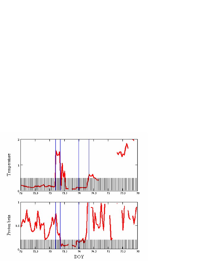
Figure 1: Temperature and proton beta decreasing under a threshold during the ICME event on 14 March 2001.

Elemental composition represents an important indicative of solar wind source and for the ICMEs presence too. Burgi and Geiss (1986) stated that the charge state information within an ICME reflects the temperature history of the CME solar counterpart. Charge state composition of elements such as O, C, and Fe, contains a coronal signature of the solar wind and extremely high charge states are associated with mass ejections. Very high charge states of Fe are considered the most reliable signature of an ICME (Lepri et al. (2001)). The $Fe/O$ abundance ratio divided by the solar $Fe/O$ ratio (about 0.05) represents a proxy for the strength of the first ionization potential fractionation. Weighted average of all charge states from $Fe(6+)$ to $Fe(16+)$ are normally between 9 and 11 in the solar wind and higher values indicate the presence of an ICME (Lepri et al. (2004)). Another signature of an ICME is the fulfilling of the condition $O(7+)/O(6+)>1$. In their study Henke et al.(Henke et al. (1998) asserted that an enhanced $O(7+)/O(6+)$ density ratio is directly correlated with magnetic clouds.

According to Burlaga, Lemaire, and Turner (1977), the magnetic clouds are also characterized by a smooth coherent rotation of the magnetic field parallel to a plane, when the spacecraft goes through the ICME considered as a flux rope. This rotation can occur in any direction on a time scale from few hours to days. These changes can be detected in the spacecraft Cartesian components of the magnetic field ($Bx,By,Bz$), where $Bx$ points from the spacecraft towards the Sun, $By$ points towards the East, and $Bz$ points normal to them towards North. The directional changes of the magnetic field can be investigated with the minimum variance method (MVA) applied to the magnetic field components in these coordinates. Klein et al. (1981) or Bothmer and Schwenn (1998) described in detail the MVA method applied to MCs.

As the CMEs propagate in the heliosphere, their internal properties and configuration change and extend, so it is difficult to relate back an ICME registered at several AU. One parameter that can be measured in-situ by satellites remains yet unchanged: this is the ionization level of the solar wind. By measuring charge states of solar wind ions, thermodynamic properties present in the source region of the solar wind can be analyzed at any distance in the heliosphere. The charge state is higher inside most of ICMEs, especially inside the magnetic clouds. Rodriguez et al. (2004) extended the analysis made by Henke et al. (1998) to a set of 40 magnetic clouds detected by Ulysses and found that the increase of the charge state is present at all latitudes and phases of solar cycle. Wurz et al. (2001) detected the elemental composition in magnetic clouds observed in 1997 and 1998. They observed that the heavy elements (carbon through iron), which can be regarded as tracers in the solar wind plasma, display a mass-dependent enrichment of ions monotonically increasing with mass. When comparing the MC plasma to regular solar wind composition, a net depletion of the lighter ions, helium through oxygen, was always observed.

3 The ICMEs propagation

One way to better understand how ICMEs evolve in the solar wind is to track specific ICMEs observed by spacecraft at different heliospheric distances. Wang et al. (2005) described the most important characteristics of the interplanetary coronal mass ejections in the heliosphere between 0.3 and 5.4 AU, using data from several spacecraft.

An excellent work was also done by Foullon et al. (2007) that investigated in detail a low latitude event coming from an active region filament and registered by more than one spacecraft. In the high-latitude ICME case we cannot perform a follow up using satellites like Ace, Wind or Helios 1 since the event is not near the ecliptic. Using data from Ulysses we could track an event occurred at high latitude and far from Earth orbit (1AU), at times when the satellite passed over the solar poles. The latitude distribution of the CMEs occurrence is solar cycle dependent and this implies that only during some periods we could expect to observe high latitude CMEs and ICMEs.

Many authors derived empirical models from observational data, concerning the CMEs propagation through heliosphere. Lindsay et al. (1999) and Gopalswamy et al. (2001) developed simple shock time of arrival models using the initial CME speed and ambient solar wind speed to predict the acceleration or deceleration of the CME. Gopalswamy et al. (2001) assumed that the CME speed remains constant from the Sun to 1 AU. Owens et al. (2004) analyzed the existing models of ICMEs travel between Sun and Earth and found a similar accuracy of the 1 AU arrival predictions of all models, eventual errors being due to the CME geometry of trajectory and expansion.

Another way to track an ICME is to observe the associated CME with a coronagraph at the solar limb and the in situ ICME with a spacecraft in quadrature with the coronagraph. It means to follow up a CME in space until it reaches a spacecraft and we get recorders from this. Demoulin (2009) showed that the slow CMEs (with $v<400$ km/s) accelerate and reach the solar wind speed, while the most rapid CMEs slow down and tend, to long distance, to the solar wind ambient speed. A similar idea is accounted by Borgazzi et al. (2008) who also took into consideration the drag force between the ICME and the solar wind. Typically the strongest deceleration occurs close to the Sun, and ICMEs have a nearly constant velocity in most of the heliosphere. Demoulin et al. (2008) analyzed the expected in situ velocities from a hierarchical model for expanding interplanetary coronal mass ejections and showed that the global acceleration of ICMEs has, at most, a small contribution to the in situ measurements of the velocity. He also analytically proved that MCs are expanding at a comparable rate, independently of their size or field strength, despite very different magnitudes in their velocity profiles.

Observations have proved that a coronal mass ejection expand into heliosphere as it travel. Simultaneous observations by widely separated spacecraft show that in large events particles reach widespread regions of the heliosphere, up to $300^{o}$ in longitude (Cliver et al. (1995)); and up to at least $80^{o}$ in latitude (Lario et al. (2003)). Energetic particle observations from interplanetary spacecraft can be used to infer the properties of the traveling CMEs. Cane et al. (1988) have shown that the proton intensity profiles of the solar energetic particle (SEP) events observed in the ecliptic plane at 1 AU are organized in terms of the longitude of the observer with respect to the traveling CME-driven shock, and resume their results in Fig. 2.

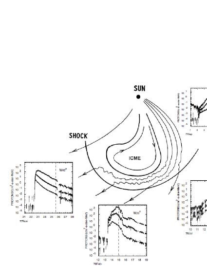
Figure 2: The shape of an ICME and surrounding interplanetary field structure including the presence of a shock (Cane et.al., 1988).

However at large heliocentric distances and at high heliolatitudes the relation between the origin of the event and the time-intensity profiles is less clear, so this result can not be applied to Ulysses observations.

Observations of the energetic particles during the passage of an ICME over the observer (spacecraft) provide valuable information about the structure of the ICME. We should distinguish the signatures of an ICME at the ecliptic level and one astronomical unity (near Earth) and those at high latitude and long distances in heliosphere. For example, an ICME passage in the ecliptic plane is associated with the energetic particle intensity depletion, known as the Forbush decreases (Cane (2000)). In contrast to this, the high-latitude ICMEs display an enhancement of the particle intensities.

4 The tracking back to the Sun

The track back to the Sun of an ICME registered at distances greater than 1 AU still remains a challenge. Several authors have identified the solar counterparts of Ulysses’ ICMEs using different methods. We remind here a few: energetic particle flux (Watari et al. (2002); Simnett (2003)), flux rope modeling (Demoulin et al. (2008)), tracking the interplanetary scintillation close to the Sun and out of ecliptic (Tokumaru et al. (2006)). Gazis et al. (2006) provided a list of works about Ulysses’ ICMEs and their solar counterparts’ determination, but this list contains events occurred until 2001.

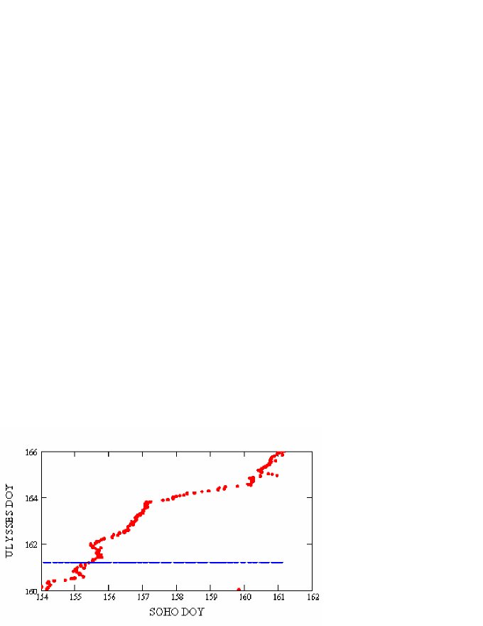
Figure 3: The track back to the Sun diagram of the ICME event from 10 June 2001 registered by Ulysses spacecraft. (Dumitrache and Popescu (2010b)).

Dumitrache (2010), Dumitrache and Popescu (2010a), Dumitrache and Popescu (2010b), Dumitrache, Popescu, and Oncica (2010), Dumitrache, Popescu, and Oncica (2011) treated the problem of the track back to the Sun of some ICME events registered by Ulysses spacecraft and identified their solar sources. They considered a linear kinematic law to track the ICME back to the Sun using the velocity registered in situ by Ulysses. Therefore they introduced a graphical method to detect the day of the year when a specific event occurred on the Sun. Fig. 3 plots a diagram with the days of the year of events registered by Ulysses on vertical axis, while on the horizontal axis are the days of the year of events should appear on the Sun and registered by SOHO. Using the CDAW catalog the authors investigated more CMEs candidates as being the solar counterpart of a specific ICME event. The dashed horizontal line marks the DOY of the ICME registered by Ulysses, so the intersection of this one with the curve of the events must give on abscise the day of the solar counterpart apparition. They also performed the follow up of all CMEs candidates registered by SOHO spacecraft until their Ulysses’ arrival. This follow up was based on a linear model but using two different velocities: first, the initial linear CMEs’ velocity, and, second, a velocity empirical formula fitted by Lindsay et al. (1999), that can be considered as the CMEs are embedded in the solar wind. Both computations indicated the same solar counterpart and the errors are of the order of hours. Formula deduced by Lindsay et al. (1999), i.e. the radial velocity ($vr$) is deduced from the initial coronograph measured velocity ($vi$), $vr=vi\cdot 0.25+360$, gives more accurate results.

Lindsay et al. (1999) studied statistical relationships between the speeds of coronal mass ejections observed near the Sun and key characteristics of the associated interplanetary disturbances (ICMEs) detected near the ecliptic at distances less than 1 AU, using a combination of Solwind and SMM coronagraph data and Helios-1 and Pioneer Venus Orbiter interplanetary field and plasma. These observations confirm that while the occurrence of large interplanetary magnetic field magnitudes and high bulk plasma speeds associated with ICME passage may be predictable from coronagraph-derived CME speeds, other important ICME features like large-magnitude southward $Bz$ require other diagnostics and tools for forecasts.

5 About the solar sources

A major step to understand the variability of the space environment is to link the sources of coronal mass ejections (CMEs) to their interplanetary counterparts or vice versa, to track back to the Sun the interplanetary disturbances and found their solar source.

A coronal mass ejection has different signatures in its core region of apparition as well as large-scale signatures by the neighborhood structures involved in. A CME can be detected by the occurrence of filament eruption or flare loop arcade, and X-ray/EUV double dimming. These signatures are observable in many wavelengths, but especially in H$\alpha$, EUV, soft X-ray and/or radio. Disturbances along coronal hole boundaries have also been reported as possible signatures of CMEs (Hudson, Acton, and Freeland (1996); Attrill et al. (2006); Veronig et al. (2006); Harra et al. (2007)).

The principal sources of CMEs are the filaments or prominences. Very often the prominences form in more complex structure where these ones are situated at the base. Above it, a coronal streamer build up, separated by a cavity. Considering the filaments classifications, we could distinguish more type of sources for the mass ejections, i.e. CME starting from polar filaments, from active regions filaments or from complex filaments.

Flares represent another important source of CMEs. Here we could distinguish also few aspects: there are flares occurring in active regions and spotless flares. However, the basic process of CMEs sources is linked to magnetic field change from quasi-static state to an erupting stage.

We remind here an interesting statistics made by Wenbin, Xueshang, and Yanqi (2007): they analyzed the solar cycle variation of the real CME latitudes. Their conclusions are that high-latitude CMEs constituted only $3\%$ of all CMEs and mainly occurred during the period of solar polar magnetic field reversal, while $4\%$ of all CMEs occurred in between $45^{0}$ and $60^{0}$ latitude. These mid-latitude CMEs occurrence presented three peaks in 2000, 2002 and in 2005. The highest occurrence rate of low-latitude CMEs (with latitude less than $45^{0}$) was at the maximum and during the declining phase of the solar cycle 23. The latitudinal evolution of low-latitude CMEs does not obey the Spörer sunspot law and this fact suggests that many CMEs originated outside of active regions and consequently to be eruptive prominences or spotless flares signatures.

Vilmer et al. (2003) analyzed and identified their solar sources for 32 interplanetary disturbances that affected the Earth. They found a large proportion to be associated with flares originating in active regions and only ten cases were associated to filament activity situated at the disk center. Other statistics, considering generally the CMEs, found that filaments are mostly sources for these explosive phenomena. VDGesztelyi synthesized the magnetic clouds characteristics and their relation to the solar sources in a comprehensive work.

Gopalswamy et al. (2010) identified a large number of interplanetary disturbances that do not have a discernable driver by the spacecraft near Earth observations. These shocks are associated with fast and wide CMEs and radio bursts type II. These CMEs were located near coronal holes. The CME-coronal hole interaction must be widespread in the declining phase of the cycle 23 and may have a significant impact on the geoeffectiveness of CMEs.

Schmieder (2006) analyzed the magnetic source regions of coronal mass ejections and revealed mainly two of them: the decaying active regions and the filaments. Usually an ICME keeps its solar source magnetic helicity. However, Chandra et al. (2010) reported the observation of a solar source with negative helicity generating a magnetic cloud with positive polarity. This magnetic cloud gave the largest geomagnetic storm of the solar cycle 23.

6 Conclusions

Many authors studied specific CME-ICMEs events and found many general properties of their in-situ identification, their propagation and evolution, but there are also many others things that make unique each event. There are also many unsolved aspects of the ICMEs diagnostic. A special class of the ICMEs is represented by the magnetic clouds, which are very important for their space weather amplified effects. The ICMEs were registered in situ by many satellites and there are few catalogues that attempted to link them to their solar sources, but the majority of these satellites are near the ecliptic and one astronomical unity (near Earth). Only Ulysses spacecraft had a unique orbit allowing registrations far from the ecliptic plane and beyond 1 AU, giving us a 3D view of the heliosphere. The tracking of a CME far than 1 AU is not an easy task and is more complicated when the events are at high-latitudes and no one additional registrations between the Sun and spacecraft can be found. For this reason the results of our PECS-ESA project (2007-2009) that focused on all these aspects represented an important step in the understanding of the CME-ICMEs events. We have analyzed in a series of articles more ICME events and their solar sources: 10 June 2001, 18 August 2001, 24 August 2001, 18 January 2002, 14 March 2002, 5 May 2002, and 15 July 2007.

References

- Attrill et al. (2006) Attrill, G., Nakwacki, M. S., Harra, L. K., van Driel-Gesztelyi, L., Mandrini, C. H., Dasso, S., Wang, J.: 2006, Sol. Phys., 238, 117.
- Borgazzi et al. (2008) Borgazzi, A., Lara, A., Romero-Salazar, L., Ventura, A.: 2008, Geofisica Internacional, 47, 301.
- Bothmer and Schwenn (1998) Bothmer, V., Schwenn, R.: 1998, \ag, 16, 1.
- Burgi and Geiss (1986) Burgi, A., Geiss, J.: 1986, Sol. Phys., 103, 347.
- Burlaga, Lemaire, and Turner (1977) Burlaga, L.F., Lemaire, J.F., and Turner, J.M.: 1977, ]jgr, 82, 3191.
- Cane et al. (1988) Cane, H. V., D. V. Reames, T. T. von Rosenvinge: 1988, J. Geophys. Res., 93, 9555.
- Cane (2000) Cane, H. V.: 2000, Space Sci. Rev., 93, 55.
- Chandra et al. (2010) Chandra R., Pariat E., Schmieder B., Mandrini C., Uddin W.: 2010, Sol. Phys., 261, 127.
- Cliver et al. (1995) Cliver, E. W., Kahler, S. W., Neidig, D. F., Cane, H. V., Richardson, I. G., Kallenrode, M.-B., Wibberenz, G.: 1995, in Proc. 24th Int. Cosmic Ray Conf., 4, 257.
- Dasso (2009) Dasso, S.: 2009, \iau, 257, eds N. Gopalswamy, D. F. Webb, 379.
- Dasso et al. (2005) Dasso, S., Mandrini, C. H., Demoulin, P., Luoni, M. L., Gulisano, A. M.: 2005, \adv, 35, 711.
- Dasso et al. (2006) Dasso, S., Mandrini, C. H., Demoulin, P., Luoni, M. L.: 2006, Astron. Astrophys., 455, 349.
- Dasso et al. (2007) Dasso, S., Nakwacki, M. S., Demoulin, P., Mandrini, C. H.: 2007, Sol. Phys., 244, 115.
- Dasso et al. (2009) Dasso, S., Mandrini, C. H., Schmieder, B., Cremades, H., Cid, C., Cerrato, Y., Saiz, E., Demoulin, P., Zhukov, A. N., Rodriguez, L., Aran, A., Menvielle, M., Poedts S.: 2009, J. Geophys. Res., 114, A02109.
- Demoulin et al. (2008) Demoulin, P., Nakwacki, M. S., Dasso, S., Mandrini, C. H.: 2008, Solar Phys., 250, 347.
- Demoulin (2008) Demoulin, P: 2008, \ag, 26, 3113.
- Demoulin (2009) Demoulin,P: 2009, \aip, 1216, 329.
- Demoulin and Dasso (2009) Demoulin, P., Dasso, S.: 2009, Astron. Astrophys., 498, 551.
- Du, Zuo, and Zhang (2010) Du, D., Zuo, P.B., and Zhang, X.X.: 2010, Sol. Phys., 262, 171.
- Dumitrache and Popescu (2009) Dumitrache, C., Popescu, N. A.: 2009, ”The 3rd Hinode Science Meeting”, Tokyo, Japan, ASP Conf. S., submitted.