Alleviating the tension at low $\ell$ through Axion Monodromy

Abstract

There exists some tension on large scales between the Planck data and the $\Lambda$CDM concordance model of the Universe, which has been amplified by the recently claimed discovery of non-zero tensor to scalar ratio $r$. At the same time, the current best-fit value of $r$ suggests large field inflation $\Delta\phi_{\rm inf}>M_{p}$, which requires a UV complete description of inflation. A very promising working example that predicts large tensor modes and can be UV completed is axion monodromy inflation. This realization of inflation naturally produces oscillating features, as consequence of a broken shift symmetry. We analyse a combination of Planck, ACT, SPT, WMAP low $\ell$ polarization and BICEP2 data, and show a long wavelength feature from an periodic potential can alleviate the tension at low multipoles with an improvement $\Delta\chi^{2}\simeq 2.5-4$ per degree of freedom, depending on the level of foreground subtraction. As with an introduction of running, one expects that any scale dependence should lead to a worsened fit at high multipoles. We show that the logarithmic nature of the axion feature in combination with a tilt $n_{s}\sim 1$ allows the fit to be identical to a no-feature model at the $2$ percent level on scales $100\leq\ell\leq 3500$, and quite remarkable actually slightly improves the fit at scales $\ell>2000$. We also consider possible unremoved dust foregrounds and show that including these hardly changes the best-fit parameters. Corrected for potential foregrounds and fixing the frequency to the best fit value, we find an amplitude of the feature $\delta n_{s}=0.095^{+0.03}_{-0.05}$, a spectral index $n_{s}=1.0^{+0.03}_{-0.04}$, the overall amplitude $\log 10^{10}A_{s}=3.06\pm 0.04$ and a phase $\phi=0.85^{+0.9}_{-1.6}$. These parameters suggest an axion decay constant of $f/M_{p}\sim\mathcal{O}(.01)$. We discuss how Planck measurements of the TE and EE spectra can further constrain axion monodromy inflation with such a large feature. A measurement of the large scale structure power spectrum is even more promising, as the effect is much bigger since the tensor modes do not affect the large scales. At the same time, a feature could also lead to a lower $\sigma_{8}$, lifting the tension between CMB and SZ constraints on $\sigma_{8}$.

I Introduction

The recent discovery of B-mode polarization in the sky BICEP2 Collaboration et al. (2014) has created enormous excitement in the community. Foremost, if the B-modes are sourced by primordial gravitational waves, the discovery can be considered additional evidence for the inflation paradigm; in the very early Universe, a yet unknown scalar field dominated the energy density in the Universe causing the Universe to expand at least $60$-efolds in a very short time. Secondly, the associated amplitude of the primordial signal is bigger than anticipated from earlier experiments, where the constraint is derived from the CMB temperature power spectrum. In a $\Lambda$CDM + $r$ concordance cosmology, Planck Planck Collaboration et al. (2013a) derived that $r_{0.05}<0.135$ at $95\%$ . The BICEP experiments derives a non-zero value of $r_{0.05}=0.2_{-0.05}^{+0.07}$, which is almost $2$ sigma away from this value. It is obvious then, that this adds to the existing tension on large angular scales between the data and the $\Lambda$CDM + $r$ concordance cosmology, as gravitational waves do not only source B-modes but also add to the scalars. Though this part of the spectrum has large cosmic variance, if the large value of $r$ persists, we will possibly have to reconsider a simple power law inflation. Naturally any power law will have some higher order deviation from scale invariance beyond the tilt. However, for any polynomial power law, the running will always be slow-roll suppressed compared to the tilt . Besides, when considering the BICEP evidence for a large $r$, a running does not lead to a significantly better fit on large scales, and at the same time it will lead to a worsened fit on small scales (see e.g. Abazajian et al. (2014); Hazra et al. (2014) for several recent attempts ). Thirdly, the large tensor to scalar ratio indicates that the field driving inflation has been displaced overall several $M_{p}$, which can be considered an issue from a model building perspective. It would be interesting if there exists a model that fits the data in 3 ways; it has naturally large tensor modes, it has some sort of running on large scales (and possibly on not yet observed small scales) and deals with super Planckian displacements in field space. In this paper we will show that such a model already exists in the form of axion monodromy inflation and it will turn out that it actually provides a significantly better fit to the data at large scales and even improves the fit on the very small scales. In addition, it makes clear testable prediction for the TE, EE and large scale structure power spectra, which should be measured with running and upcoming experiments. Interestingly, a large feature also lowers the derived value of $\sigma_{8}$, relieving some of the tension with measurements of $\sigma_{8}$ using the SZ signal Planck Collaboration et al. (2013b).

This paper is organized as follows. We will briefly give a theoretical background and motivation to consider a large scale (i.e. long wavelength) feature in light of the recent BICEP2 measurements in §II. In §III, we present our results and show that a long wavelength feature provides an improved fit to the data. We will consider the most pessimistic foreground models derived in BICEP2 Collaboration et al. (2014) in combination with large and small scale CMB experiments. Our findings will be discussed in §IV, where we will present some simple estimate of how much a large feature could be due to cosmic variance. In addition, we will discuss the possible implications for EE and TE polarization as well the matter power spectrum. We conclude in §V.

II Theoretical Background

Under the assumption that the discovery of non-zero B-modes in the CMB sky BICEP2 Collaboration et al. (2014) is caused by the production of primordial gravitational waves (see Flauger et al. (2014) for a thorough discussion on this topic), together with the COBE normalization $\delta_{H}\simeq 1.9\times 10^{-9}$ we can infer the scale of inflation

$$\Lambda\simeq\left(\frac{r}{0.2}\right)^{1/4}2.4\;10^{16}\;{\rm Gev},$$ (1)

which implies $\Lambda\sim 10^{16}$ GeV for the current measured $r\simeq 0.2$. In addition, besides a measurement of $V=\Lambda^{4}$, through $r=16\epsilon$, and $\epsilon\propto(V^{\prime}/V)^{2}$, we also learn about $V^{\prime}$. As such, the detection of $B$-modes has already allowed one to limit the number of inflationary models, while the simplest model has persisted. However simple, the measurement of large $r$ has implications for inflation beyond the presence of primordial gravitational waves. According to the Lyth bound (Lyth and Riotto, 1999; Easther et al., 2006)

$$\Delta\phi_{\rm inf}\geq M_{p}\sqrt{\frac{r}{4\pi}}.$$ (2)

The bound is valid for slow-roll single-field inflationary models but can be generalized (Baumann and Green, 2012). The main idea is that the production of observable gravitational waves can only be accomplished during inflation if the field driving inflation displaces over super Planckian distances, during the time the observable scales exit the horizon. This approximate theoretical bound poses a challenge for model builders, as it requires one to fully formalize a model that is UV complete; the absence of such prescription, would introduce an infinite fine tuning of higher order operators. Although this is only a theoretical complaint, it is considered unsatisfying and to some extend nonpredictive, arguably driving us towards an anthropic point of view; the precise cancelation of higher order terms can only be explained by assuming that enough E-folds of inflation would not have occurred without it and hence, we would have not been here to observe it.

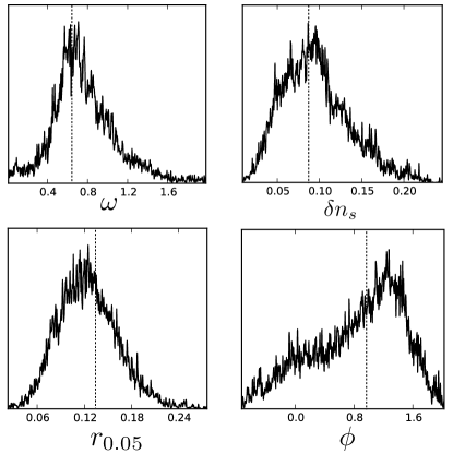
Figure 1: Marginalized posterior probability distribution for $\omega$, $\delta n_{s}$, $r_{0.05}$ and the phase $\phi$ derived from Planck+Lensing+WP+high $\ell$+BICEP-DDM2. The dashed line is the best fit value, which coincides reasonably well with the marginalized values.

Although other models exist Liddle et al. (1998); Dimopoulos et al. (2008), a thoroughly investigated UV-complete model known as axion monodromy Kim et al. (2005); Silverstein and Westphal (2008); McAllister et al. (2010); Flauger et al. (2010), originally motivated by natural inflation Freese et al. (1990), can currently be considered as one of the few examples that addresses super Planckian displacements. Derived within string theory, monodromy models unwrap angular directions in field space, and have monomial potentials over super-Planckian distance . The shift symmetry of the model is broken non-perturbatively to a discrete shift symmetry which results in an sinusodal feature in the potential . The resulting power spectrum can be approximated by a power law modified with logarithmically spaced osculations. In our analysis we will use the parametric form (scalars)

$$\Delta^{2}_{\mathcal{R}}(k) = A_{s}\left(\frac{k}{k_{*}}\right)^{n_{s}-1}\left(1+\delta n_{s}\cos[\omega\log k/k_{*}+\phi]\right),$$

and for the tensors (see the appendix for a derivation)

$$\Delta^{2}_{\mathcal{D}}(k) = A_{s}\frac{r_{*}}{4}\left(\frac{k}{k_{*}}\right)^{-r_{*}/8}\left(1-\delta n_{s}\frac{r_{*}}{8\omega}\sin[\omega\log k/k_{*}+\phi]\right).$$

Specifically, for axion monodromy inflation $\omega=\sqrt{2\epsilon_{*}}/f=\sqrt{r_{*}}/(f\sqrt{8})$, with $f$ the axion decay constant. The oscillatory term in Eq. (LABEL:eq:tensorspectra) is generally subleading, since it suppressed by a factors of $r_{*}$, and one power of the frequency. For $f<M_{p}$ (note that $[f]=M_{p}^{\rm red}$) and $r\sim 10^{-1}$, we have $\omega\gtrsim 10^{-2}$. Hence, at best, such a level of primordial gravitional waves suggest oscillations in the tensor modes are suppressed with respect to those in the scalar spectrum by about an order of magnitude. In fact, the suppression is always $\sqrt{r_{*}}f$, and hence one expects this term to be subdominant unless $f*M_{p}^{\rm red}>M_{p}$.

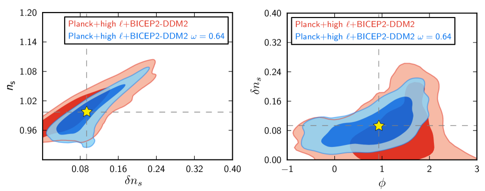
Figure 2: 2 Dimensional posterior probability distribution for $n_{s}$ vs $\delta n_{s}$ (left) and $\phi$ vs $\delta n_{s}$ (right). The stars represent the best fit points. The contours in red shades are derived from the chains with a prior on $\omega$ as specified in the text, while the blue shaded contours are derived from a chain with a set value for the frequency, close to the best fit value found using the previous chains. In the left it is clear that he tilt and amplitude are highly correlated; effectively the long wavelength oscillation acts a a tilt on low multipoles.

Note that the above paramaterization also puts a constraint on the priors; the spectrum could become negative if the amplitude were to become too large. The results presented here are derived in the assumption that the oscillations are small. We put a prior on the amplitude $0\leq\delta n_{s}\leq 0.3$, $0\leq r\leq 0.4$ and $0.01\leq\omega\leq 2$, where the latter upper limit is somewhat arbitrary as axion monodromy does allow for higher frequency oscillations. Since we are only interested in at most a single oscillation to account for power suppression at large scales, we decided to cut off the frequency at this value, which roughly corresponds to 1 oscillation in the observed CMB. It can also be shown that oscillations with a frequency lower than this will be strongly correlated with other primordial parameters, while the correlation mostly disappears for higher frequencies, which favors a dedicated search varying all cosmological parameters at these low frequencies.

This parametric form (without the tensor part) has been investigated in multiple publications Flauger et al. (2010); Meerburg et al. (2012); Easther and Flauger (2013); Meerburg et al. (2014a, b, c), while Peiris et al. (2013) computed the exact numerical power spectrum directly from the potential. For further background on the details of axion monodromy inflation we would like to refer the reader to these excellent reviews Pajer and Peloso (2013) and more generally Baumann and McAllister (2014). Other models that introduce logarithmic oscillations in the primordial power spectrum include e.g. models with a modified initial state Greene et al. (2005), unwinding inflation D’Amico et al. (2013) and cascade inflation Ashoorioon et al. (2009). Recent attempts to look for features in the CMB data can be found in e.g. Refs. Meerburg et al. (2012); Achúcarro et al. (2014); Hazra et al. (2013).

III Results

Data set \Parameter	$\Omega_{b}h^{2}$	$\Omega_{c}h^{2}$	$\tau$	$H_{0}$	$n_{s}$	$\log 10^{10}A_{s}$	$\delta n_{s}$	$\phi$	$\omega$	$r_{0.05}$	$\Delta\chi^{2}$
Planck+high $\ell$ + BICEP2	$0.022$	0.119	0.096	67.54	1.004	3.082	0.0743	1.28	0.802	0.21	$\sim 11$
Planck+high $\ell$ + BICEP2 - DDM2	$0.022$	0.119	0.098	67.74	0.997	3.076	0.09	0.93	0.64	0.13	$\sim 7$

Table 1: Best-fit parameters for various data combinations. Note the tilt is $n_{s}\simeq 1$ in order to account for effects on small scales due to the long wavelength oscillation. Subtracting potential foregrounds does not significantly change the parameter values, nor the significance.

In light of the observed level of B-modes, as well as the presence of a slight tension at large scales between the data and the theory, we performed an analysis of the BICEP2 data BICEP2 Collaboration et al. (2014) in combination with the Planck public likelihood Planck collaboration et al. (2013) and a modified version of the public cosmology package Cosmomc Lewis and Bridle (2002). We also included small scale CMB data from the ACT Das et al. (2014) and SPT Keisler et al. (2011); Reichardt et al. (2012) experiments. Data from these experiments act as an extension of the leverage arm, suppressing large deviations from scale invariance (which is not preferred by these experiments). As we will see however, the best fit model does not affect the small scale power spectrum on CMB scales, but does affect the matter power spectrum, both on large scales and on small scales.

Regarding the BICEP measurement, we will include a no-foreground, as well as foreground corrected analysis, where the latter is taken from the BICEP paper (the data-drives models, auto DDM1, and cross DDM2 spectra BICEP2 Collaboration et al. (2014)). We use the standard Metropolis-Hasting sampling, and vary all parameters, including Planck foregrounds. Because of the high irregularity of the likelihood in the frequency direction, such a chain will never converge according to the $R-1$ convergence test. However, we terminate the chain by considering the convergence of each troubled parameter has reached $R-1<0.1$. It must be noted, that the derived distributions are not a very accurate representation of the true distribution, as parts of the likelihood will be oversampled. The significance bounds we quote are derived from an analysis where we fixed the frequency to its best-fit value, derived from a sampling that included the frequency as a free parameters as described above. We also investigated using the nested sampler Multinest Feroz et al. (2009, 2013), however we found that including high $\ell$ data, oscillations and BICEP2 data resulted in very slow convergence. For our low $\ell$ analysis with fixed foregrounds we recover the same results as with the Metropolis-Hastings sampling, providing confidence in our obtained results using the MH sampler. Simply looking for the best-fit point also proofed troublesome, as existing methods are quite sensitive to the initial search volume.

Figure 1 shows an example of a 1D marginalized distribution derived from $Planck$ + high $\ell$+ $BICEP2$, where the latter has been corrected for foregrounds using the DDM2 dust model. The dashed lines represent the best-fit values of the 4 parameters. We obtained the distribution for $\omega$ from varying all parameters, and the other 3 have been obtained by fixing the frequency to the best-fit value. We find $\delta n_{s}=0.095^{+0.03}_{-0.05}$, $n_{s}=1.0^{+0.03}_{-0.04}$, $\log 10^{10}A_{s}=3.06\pm 0.04$ and $\phi=0.85^{+0.9}_{-1.6}$.

In Fig. 2 we show the marginalized 2 dimensional contours between $n_{s}$ and the amplitude (left) and $\phi$ and the amplitude (right). The two contours in each plot are derived from the combination of Planck, SPT, ACT and foreground corrected BICEP data. The figure on the left shows that the tilt and the amplitude are correlated, which is unsurprising since the long wavelength oscillation + associated amplitude can replace the scale dependence coming from the tilt. In Table 1 we show the best-fit parameters derived from foreground cleaned and uncleaned analysis. Interestingly we find a best-fit value of $n_{s}\sim 1$, i.e. close to a scale invariant form of the non-oscillating part of the potential. We will discuss this in the next section.

component	$\Delta\chi^{2}$
Lowlike	$\sim-0.3$
Lensing	$\sim 0.6$
BICEP2	$\sim-3.4$
Commander	$\sim-8$
CAMspec	$\sim 1.1$
ACTSPT	$\sim-1.2$
total	$\sim-11.2$

Table 2: $\Delta\chi^{2}$ breakdown per component for the analysis of the axion model versus concordance model without foreground corrections. The improvement is most significant in commander and in BICEP2 as expected. Note also that there is small improvement in the high $\ell$ fit. Including foreground subtraction, the improvement in commander and BICEP are lowered.

IV Discussion

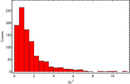
Figure 3: Distribution of $\chi^{2}$ improvements simulating 1000 Universes and fitting for a feature on $\ell<1000$. This simple analysis suggest that cosmic variance can account for $\Delta\chi^{2}\sim 2$.

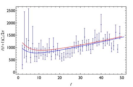
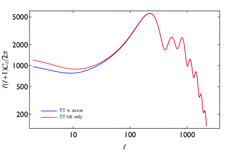
Figure 4: The best fit TT spectrum for a concordance cosmology (red) and the axion monodromy fitted model (blue). These plots are generated using the parameters derived from Planck+high $\ell$+lensing+WP+BICEP data.

In previous work Easther and Flauger (2013); Meerburg et al. (2014a) it was investigated to what extent the noise + cosmic variance can mimic a feature . It was shown that for a broad prior on the frequency, improvements are generally expected around $\Delta\chi^{2}=10$ making any improvement of this order in the data suspicious. The relatively small improvement here suggests we should worry about a fitting to the noise. However, as can be imagined, it becomes much harder to fit to the noise with a long wavelength feature, because points are correlated over a large range of scales (something that in principle the noise should not be). In Fig. 3 we show the resulting distribution from a simple analysis where we try to fit an oscillation to the TT spectrum with cosmic variance an Planck-like noise, varying only the amplitude and the phase of a fixed feature. We only consider up to $\ell=1000$, since we are interested in the improvement at low multipole. This simple analysis suggests that the noise alone can not account for a fit, given that the typical improvement from cosmic variance + noise os of the order $\Delta\chi^{2}\sim 2$. Unlike for high frequencies therefore, a long wavelength modulation follows a typical $\chi^{2}$ distribution for $\sim 2$ parameters, which is not unexpected given the nature of the modulation (an effective rescaling of the amplitude).

In Table 2 we break down the contribution to the improved $\Delta\chi^{2}$. The nature of the feature would suggest the improvement is dominated by large scales, hence by the commander component of the likelihood, which captures $\ell\leq 50$. It is reassuring to see that for the the contribution is indeed dominated by the commander likelihood as well as the BICEP2 likelihood (which causes the tension). At the same time, the likelihood at small scales is effectively unchanged.

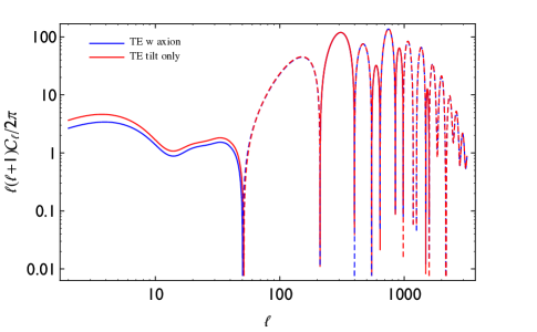
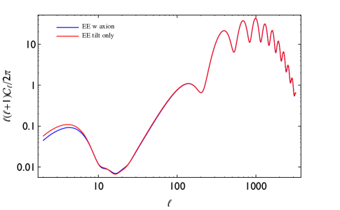
Figure 5: The best fit TE (left) and TT(right) spectrum for a concordance cosmology (red) and the axion monodromy fitted model (blue). These plots are generated using the parameters derived from Planck+high $\ell$+lensing+WP+BICEP data. For TE, the difference for the range $\ell=2-40$ is of order 20$\%$ for EE on the same range, the difference is about 10$\%$.

In Fig. 4 we show the best fit TT spectrum from this analysis and we compare this with the best fit concordance cosmology. Quite interestingly, the resulting plot has a strong overlap at all $100\leq\ell\leq 3500$. The larger value of the tilt compensates for any deviations at large $\ell$ from the oscillation. In Fig. 5 we show the anticipated difference with the EE and TE spectra. The difference between the concordance model for TE is relatively largest, and a Planck polarization measurements might be able to give further evidence for a large feature. These are relatively large scales, so they are cosmic variance limited. For TE over the range $\ell=2-40$ the difference is about 20$\%$. We can estimate a detection by computing the signal to noise of the difference, i.e. for a full sky experiment

$$\left(S/N\right)^{2}\simeq\sum_{\ell=2}^{40}(2\ell+1)\frac{(C^{\rm tilt}_{\ell}-C_{\ell}^{\rm axion})^{2}}{(C_{\ell}+N_{\ell})^{2}}$$ (5)

Given the difference of around $20\%$, and in the assumption we are limited by cosmic variance, we obtain $S/N\sim 8$, i.e. such a difference should be detectible. If one includes noise (which will be there for Planck) and the fact that for cosmology the sky fraction is about 30$\%$, we expect that Planck will be near the detection limit. What should be emphasized is that this simple estimate shown that a combined analysis of TT, TE and EE would help discriminate between the axion model and concordance cosmology.

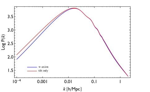
Figure 6: The best fit matter spectrum for a concordance cosmology (red) and the axion monodromy fitted model (blue) at redshift $z=1.5$. These plots are generated using the parameters derived from Planck+high $\ell$+lensing+WP+BICEP data.

In Fig. 6 we also show the matter power spectrum. At linear order the matter power spectrum is not affected by tensor modes, so the difference with the concordance model is much bigger as shown in the left panel of Fig. 7. In theory therefore, a measurement of the matter power spectrum at large scales would be the ideal way to constrain features on large scales. At very small scales, the model should start to deviate again, and a measure of small scales could further constrain a feature model. Interestingly, note that a feature also lowers the derived value of $\sigma_{8}$, putting it closer to the value estimated from $SZ$ measurements. We show the projected error of WFIRST on the right panel in Fig. 7. From this projection WFIRST Spergel et al. (2013) should be able to distinguish a feature for modes $k\geq 10^{-2}$ Mpc^-1.

V Conclusion

Figure 7: (Left) The ratio of the measured power spectra with $r$ and $r+$ axion monodromy. We also show the contribution from the tensor modes only (which actually gives a positive contribution) with the aim of showing that the tensor are not contributing to the matter power spectrum and deviations from scale invariance of the form presented in this paper should be best constraint with a large scale measure of the matter power at redshift $z=1.5$. (Right) The projected detection of a feature in the large scale power spectrum with a spectroscopic galaxy survey with a volume $21$ Gpc³ such as WFIRST Spergel et al. (2013).

In this short paper we considered the novel possibility that a feature at large scales exists, alleviating marginal existing tension between the data and the $\Lambda$CDM concordance cosmology. Such a feature can be produced by various models, but in light of the super Planckian displacement of the field, the axion monodromy model appears to be a very interesting candidate. Although the predicted signal of such a model should produce a feature that persists even to the smallest scales, the logarithmic nature of the feature does not violate any measurements at small scales for very long wavelengths. We find that both $Planck+BICEP$ as well as the inclusion of small scale measurements of the CMB from $ACT$ and $SPT$, prefer such a feature and give an improvement of $\Delta\chi^{2}\sim 11$. This result is obtained from taking the BICEP data at face value and not correcting for foregrounds. We are however seriously concerned by the foregrounds and if we include the most optimistic foregrounds model, the improvement is reduced, but parameters are hardly affected.

We have also shown that such a feature cannot be the result of cosmic variance, hence if the $BICEP$ findings are real, a feature of this type could persist. We discussed the potential of $Planck$ polarization measurements as a possible way to confirm of debunk such a feature in the near future. We also showed that because the matter power spectrum is not affected by tensors, the deviation at large scales from the concordance model would be bigger and WFIRST should be able to test the presence of such a feature with high significance. At the same time, a suppression of the matter power spectrum leads to a smaller value of the derived $\sigma_{8}$.

The fitted feature introduces 3 additional parameters, we find that the best-fit tilt is close to 1, and the feature can take care of all the scale dependence within the observed window. Hence, one could argue, that at least within the observed window, one needs only 2 additional parameters. Obviously, this would require a model that naturally explains $n_{s}=1$ (i.e. no power law scale dependence). We acknowledge that such a model would most likely be fine tuned and we should really count all 3 additional degrees of freedom if we want to address the significance of the improvement. Quite surprisingly, the large tilt in combination with the feature, agrees excellently with the small scale measurements from $ACT$ and $SPT$, resulting to a spectrum that differs $<2\%$ for $100\leq\ell\leq 3200$ and does not worsen the fit at (the observed) small scales, a handicap of most models that try to alter the spectrum on large scales.

The intriguing possibility exists that the data prefers an axion monodromy inflation scenario, with $f/M_{p}\simeq 0.01$ . The model has the advantage of being UV complete and there is no need for fine-tuning. That being said, in principle the theoretical prior on the axion decay constant is weak and for completeness one should include all possible frequencies. Here we decided to focus on the low frequency end, since the new information in the form of a non-zero tensor-to scalar ratio will most likely not change the conclusion drawn in e.g. Easther and Flauger (2013); Meerburg et al. (2014a); i.e. there is no compelling evidence for high oscillatory features in the CMB data. A problem with the current constraint is that the best-fit tensor to scalar ratio is rather large, and possibly too large for axion monodromy (although a new proposal results in larger values McAllister et al. (2014)). At the same time a tilt that close to $1$ is hard to achieve (although, naturally, for axion monodromy the tilt is closer to 1 than what is measured without a modulation). However, it is very plausible that future data, including a better understanding of the foregrounds will lower the value of $r$ and this would probably also lead to a tilt that is more consistent with axion monodromy potentials. This is already apparent from the simple analysis we have done here, where we subtracted data driven foreground models from the BB spectrum. The foregrounds subtraction indeed lowers $r$ and $n_{s}$ bringing them closer to theoretically predicted values. At the same time, the significance is lowered because the tension between the data and the concordance model is weakened. Ultimately, a full understanding of the foregrounds is necessary in order to address the evidence of axion monodromy inflation, which could be a serious concern Flauger et al. (2014). We hope to report on this in future work.

Appendix A Scalar and tensor power spectra for large modulations.

The axion monodromy potential is given by

$$V(\phi) = V_{0}(\phi)+\Lambda^{4}\cos\left(\frac{\phi}{f}\right),$$ (6)

where $\phi$ is a canonically normalized scalar field and $V_{0}(\phi)$ is the slow-roll potential in the absence of modulations. A model with a linear potential has been derived from string theory, but for the remainder of this derivation will not be specifically considered. $\Lambda$ and $f$ have the dimensions of mass. One can define a monoticity parameter

$$b_{*}\equiv\frac{\Lambda^{4}}{V^{\prime}(\phi_{*})f}<1,$$ (7)

which sets the requirement that the potential is monotonic for the scales observed the the CMB. The monoticity parameter is computed at $\phi=\phi_{*}$ when the mode $k=k_{*}$ exists the horizon. We will be using the following Hubble slow-roll parameters

$$\epsilon\equiv-\frac{\dot{H}}{H^{2}}\;\;\;\delta\equiv\frac{\ddot{H}}{2\dot{H}H}.$$ (8)

One can derive a the time dependence of the scalar field from the potential

$$\phi(t) = \phi_{0}(t)-\frac{3b_{*}f^{2}}{\sqrt{2\epsilon_{*}}}\sin\left(\frac{\phi_{0}(t)}{f}\right),$$ (9)

where $\epsilon_{*}$ is the slow-roll parameter in the absence of modulations evaluated at $\phi_{0}=\phi_{*}$. We expend the slow-roll parameters in power of the monoticity parameter (which has to be small)

$$\epsilon=\epsilon_{0}+\epsilon_{1}+\mathcal{O}(b_{*}^{2}),$$ (10)

$$\delta=\delta_{0}+\delta_{1}+\mathcal{O}(b_{*}^{2}).$$ (11)

In the slow-roll approximation for the unmodulated field $\phi_{0}$ and

$$\epsilon_{0} = \epsilon_{*}$$ (12)

$$\epsilon_{1} = -3b_{*}\frac{f\sqrt{2\epsilon_{*}}}{1+(3f/\sqrt{2\epsilon_{*}})^{2}}\left[\cos\left(\frac{\phi_{0}}{f}\right)+\right.$$ (13)

$$\left.(3f/\sqrt{3\epsilon_{*}})\sin\left(\frac{\phi_{0}}{f}\right)\right],$$

$$\delta_{1} = -3b_{*}\frac{1}{1+(3f/\sqrt{2\epsilon_{*}})^{2}}\left[\sin\left(\frac{\phi_{0}}{f}\right)-\right.$$ (14)

$$\left.(3f/\sqrt{3\epsilon_{*}})\cos\left(\frac{\phi_{0}}{f}\right)\right].$$

One can compute the scalar perturbations and the tensor perturbations as follows. We pick the following gauge

$$\delta g_{ij}({\bf x},t) = 2a(t)^{2}\mathcal{R}({\bf x},t)\delta_{ij},$$ (15)

and

$$\mathcal{R}({\bf x},t) = \int\frac{d^{3}{\bf k}}{(2\pi)^{3}}\mathcal{R}({\bf k},t)e^{i{\bf k}\cdot{\bf x}}.$$ (16)

The most general solution $\mathcal{R}$ in case of rotational invariance and hermiticity can be written as

$$\mathcal{R}({\bf k},t) = \mathcal{R}_{k}a({\bf k})+\mathcal{R}_{k}^{*}a^{\dagger}(-{\bf k}),$$ (17)

where the creation and annihilation operators satisfy the usual commutation relations

$$\left[a({\bf k}),a^{\dagger}({\bf k}^{\prime})\right] = (2\pi)^{3}\delta({\bf k}-{\bf k}^{\prime}).$$ (18)

The Mukhanov-Sasaki equation can be written as

$$\frac{d^{2}\mathcal{R}_{k}}{dx^{2}}-\frac{2(1+2\epsilon+\delta)}{x}\frac{d\mathcal{R}_{k}}{dx}+\mathcal{R}_{k} = 0,$$ (19)

with $x=-k\tau$ and $\tau$ the conformal time. In de Sitter, the infinite past lies at $\tau\rightarrow-\infty$ and the initial conditions are such that

$$\mathcal{R}_{k}(x)\rightarrow-\frac{H}{\sqrt{2k}a\dot{\phi}}e^{ix}.$$ (20)

In the future, $\tau\rightarrow 0$ and the mode functions $R_{k}$ approach a constant which will be donated by $\mathcal{R}^{(0)}_{k}$. The associated spectrum of perturbations is related to $\mathcal{R}_{k}$ as

$$\left|\mathcal{R}^{(0)}_{k}\right|^{2}=(2\pi)^{2}\frac{\Delta_{\mathcal{R}}^{2}(k)}{k^{3}}.$$ (21)

For tensors we can derive a similar equation Weinberg (2008)

$$\frac{d^{2}\mathcal{D}_{k}}{dx^{2}}-2\frac{1+\epsilon}{x}\frac{d\mathcal{D}_{k}}{dx}+\mathcal{D}_{k} = 0.$$ (22)

In Flauger et al. (2010) it was shown that the quantity of interest to first order in $b_{*}$ is given by

$$\left|\mathcal{R}^{(0)}_{k}\right|^{2} = \left|\mathcal{R}^{(0)}_{k,0}\right|^{2}\left[1+2{\rm Re}g_{1}(0)\right],$$ (23)

for scalars and

$$\left|\mathcal{D}^{(0)}_{k}\right|^{2} = \left|\mathcal{D}^{(0)}_{k,0}\right|^{2}\left[1+2{\rm Re}g_{2}(0)\right],$$ (24)

for tensors. $\left|\mathcal{R}^{(0)}_{k,0}\right|^{2}$ and $\left|\mathcal{D}^{(0)}_{k,0}\right|^{2}$ are the solutions without modulations as in Eq. (21), and the correction obey the Mukhanov-Sasaki equations

$$\frac{d^{2}g_{1,2}}{dx^{2}}-\frac{2}{x}\frac{dg_{1,2}}{dx}+g_{1,2}=2e^{ix}S_{1,2},$$ (25)

with $S_{1}=2\epsilon_{1}+\delta_{1}$ for scalars and $S_{2}=\epsilon_{1}$ for tensors. We will work to leading order in slow-roll for tensors and scalars, dropping the contribution from $\epsilon$ for scalars.

Using trigonometric identities, one can show that

$$\epsilon_{1} = \frac{-3b_{*}f\sqrt{2\epsilon_{*}}}{\sqrt{1+(3f/{\sqrt{2\epsilon_{*}})^{2}}}}\sin\left(\frac{\phi_{0}(x)}{f}+\psi\right),$$ (26)

$$\delta_{1} = \frac{3b_{*}}{\sqrt{1+(3f/{\sqrt{2\epsilon_{*}})^{2}}}}\cos\left(\frac{\phi_{0}(x)}{f}+\psi\right).$$ (27)

with $\psi=\arcsin\left[(1+(3f/\sqrt{2\epsilon_{*}})^{2})^{-1/2}\right]$. Here we will neglect this phase, since it will be unimportant and in the search for modulations in the data, we only care about the relative phase between the tensor and scalar modulations.

Using the relation $\phi_{0}(x)=(2\epsilon_{*})^{-1/2}-(2\epsilon_{*})^{1/2}\ln(k/k_{*})=\phi_{k}+(2\epsilon_{*})^{1/2}\ln x$, and $r_{1,2}(x)\equiv{\rm Re}(g_{1,2}(x))$ we write the Mukhanov-Sasaki equations for the scalars as

$$\frac{d^{2}r_{1}}{dx^{2}}-\frac{2}{x}\frac{dr_{1}}{dx}+r_{1}=\frac{6b_{*}}{\sqrt{1+(3f/{\sqrt{2\epsilon_{*}})^{2}}}}\cos(x)\cos\left(\phi_{k}/f+\sqrt{2\epsilon_{*}}\ln x/f\right),$$ (28)

and for tensors

$$\frac{d^{2}r_{2}}{dx^{2}}-\frac{2}{x}\frac{dr_{2}}{dx}+r_{2}=\frac{-6b_{*}f\sqrt{2\epsilon_{*}}}{\sqrt{1+(3f/{\sqrt{2\epsilon_{*}})^{2}}}}\cos(x)\sin\left(\phi_{k}/f+\sqrt{2\epsilon_{*}}\ln x/f\right).$$ (29)

The solutions can be found using Green’s functions. We are interested in the solution at late times when $x\rightarrow 0$. Following Flauger et al. (2010) and Flauger and Pajer (2011) we find up to a phase

$$r_{1}(0)=\delta n_{s}\cos\left(\frac{\phi_{k}}{f}\right),$$ (30)

and

$$r_{2}(0)=-f\sqrt{2\epsilon_{*}}\delta n_{s}\sin\left(\frac{\phi_{k}}{f}\right),$$ (31)

with

$$\delta n_{s} = \frac{12b_{*}}{\sqrt{1+(3f/{\sqrt{2\epsilon_{*}})^{2}}}}\sqrt{\frac{\pi}{8}\coth\left(\frac{\pi\sqrt{2\epsilon_{*}}}{2f}\right)\frac{f}{\sqrt{2\epsilon_{*}}}}.$$

Note that compared to the scalar power spectrum, the tensor modulation is suppressed in amplitude with a factor $\frac{\sqrt{2\epsilon_{*}}}{f}>1$. We can use the definition of the tensor to scalar ratio (note there are 2 helicity modes for the tensors)

$$r_{k}\equiv 4\left|\mathcal{D}^{(0)}_{k}\right|^{2}/\left|\mathcal{R}^{(0)}_{k}\right|^{2},$$ (33)

and for the power law of the potential $r=16\epsilon$ or, for a fixed pivot scale $r_{*}=16\epsilon_{*}$. We can thus write down our power spectra as

$$\Delta_{\mathcal{R}}^{2}(k)=\Delta_{\mathcal{R}}^{2}(k_{*})\left(\frac{k}{k_{*}}\right)^{n_{s}-1}\left[1+\delta n_{s}\cos\left(\frac{\phi_{k}}{f}\right)\right],$$

and

$$\Delta_{\mathcal{D}}^{2}(k)=\frac{r_{*}}{4}\Delta_{\mathcal{R}}^{2}(k_{*})\left(\frac{k}{k_{*}}\right)^{-r_{*}/8}\left[1-\delta n_{s}\frac{(r_{*}^{1/2}f)}{(8)^{1/2}}\sin\left(\frac{\phi_{k}}{f}\right)\right].$$

We can use these expressions to build consistent templates

$$\Delta^{2}_{\mathcal{R}}(k) = A_{s}\left(\frac{k}{k_{*}}\right)^{n_{s}-1}\left(1+\delta n_{s}\cos[\omega\log k/k_{*}+\phi]\right),$$

$$\Delta^{2}_{\mathcal{D}}(k) = A_{s}\frac{r_{*}}{4}\left(\frac{k}{k_{*}}\right)^{-r_{*}/8}\left(1-\delta n_{s}\frac{r_{*}}{8\omega}\sin[\omega\log k/k_{*}+\phi]\right).$$

Note that the term is subleading term in the scalars (i.e. $\propto\epsilon$) is of the same order as the tensors. However, in the derivation of the equation of motion, terms of the same order have been dropped and these terms are suppressed by almost 2 orders of magnitude for $\omega\sim 1$ (the frequency range of interest for a long wavelength modulation).

References

- BICEP2 Collaboration et al. (2014) BICEP2 Collaboration, P. A. R. Ade, R. W. Aikin, D. Barkats, S. J. Benton, C. A. Bischoff, J. J. Bock, J. A. Brevik, I. Buder, E. Bullock, et al., ArXiv e-prints (2014), eprint 1403.3985.
- Planck Collaboration et al. (2013a) Planck Collaboration, P. A. R. Ade, N. Aghanim, C. Armitage-Caplan, M. Arnaud, M. Ashdown, F. Atrio-Barandela, J. Aumont, C. Baccigalupi, A. J. Banday, et al., ArXiv e-prints (2013a), eprint 1303.5076.
- Abazajian et al. (2014) K. N. Abazajian, G. Aslanyan, R. Easther, and L. C. Price, ArXiv e-prints (2014), eprint 1403.5922.
- Hazra et al. (2014) D. K. Hazra, A. Shafieloo, G. F. Smoot, and A. A. Starobinsky, ArXiv e-prints (2014), eprint 1404.0360.
- Planck Collaboration et al. (2013b) Planck Collaboration, P. A. R. Ade, N. Aghanim, C. Armitage-Caplan, M. Arnaud, M. Ashdown, F. Atrio-Barandela, J. Aumont, C. Baccigalupi, A. J. Banday, et al., ArXiv e-prints (2013b), eprint 1303.5080.
- Flauger et al. (2014) R. Flauger, J. C. Hill, and D. N. Spergel, ArXiv e-prints (2014), eprint 1405.7351.
- Lyth and Riotto (1999) D. H. Lyth and . A. Riotto, Phys. Rep. 314, 1 (1999), eprint hep-ph/9807278.
- Easther et al. (2006) R. Easther, W. H. Kinney, and B. A. Powell, J. Cosm. Astropart. Phys. 8, 004 (2006), eprint astro-ph/0601276.
- Baumann and Green (2012) D. Baumann and D. Green, J. Cosm. Astropart. Phys. 5, 017 (2012), eprint 1111.3040.
- Liddle et al. (1998) A. R. Liddle, A. Mazumdar, and F. E. Schunck, Phys.Rev. D58, 061301 (1998), eprint astro-ph/9804177.
- Dimopoulos et al. (2008) S. Dimopoulos, S. Kachru, J. McGreevy, and J. G. Wacker, J. Cosm. Astropart. Phys. 8, 003 (2008), eprint hep-th/0507205.
- Kim et al. (2005) J. E. Kim, H. P. Nilles, and M. Peloso, J. Cosm. Astropart. Phys. 1, 005 (2005), eprint hep-ph/0409138.
- Silverstein and Westphal (2008) E. Silverstein and A. Westphal, Phys. Rev. D 78, 106003 (2008), eprint 0803.3085.
- McAllister et al. (2010) L. McAllister, E. Silverstein, and A. Westphal, Phys. Rev. D 82, 046003 (2010), eprint 0808.0706.
- Flauger et al. (2010) R. Flauger, L. McAllister, E. Pajer, A. Westphal, and G. Xu, J. Cosm. Astropart. Phys. 6, 009 (2010), eprint 0907.2916.
- Freese et al. (1990) K. Freese, J. A. Frieman, and A. V. Olinto, Phys. Rev. Lett. 65, 3233 (1990), URL http://link.aps.org/doi/10.1103/PhysRevLett.65.3233.
- Meerburg et al. (2012) P. D. Meerburg, R. A. M. J. Wijers, and J. P. van der Schaar, Mon. Not. R. Astron. Soc. 421, 369 (2012), eprint 1109.5264.
- Easther and Flauger (2013) R. Easther and R. Flauger, ArXiv e-prints (2013), eprint 1308.3736.
- Meerburg et al. (2014a) P. D. Meerburg, D. N. Spergel, and B. D. Wandelt, Phys. Rev. D 89, 063536 (2014a), eprint 1308.3704.
- Meerburg et al. (2014b) P. D. Meerburg, D. N. Spergel, and B. D. Wandelt, Phys. Rev. D 89, 063537 (2014b), eprint 1308.3705.
- Meerburg et al. (2014c) P. D. Meerburg, D. N. Spergel, and B. D. Wandelt, ArXiv e-prints (2014c), eprint 1406.0548.
- Peiris et al. (2013) H. Peiris, R. Easther, and R. Flauger, ArXiv e-prints (2013), eprint 1303.2616.
- Pajer and Peloso (2013) E. Pajer and M. Peloso, Classical and Quantum Gravity 30, 214002 (2013), eprint 1305.3557.
- Baumann and McAllister (2014) D. Baumann and L. McAllister, ArXiv e-prints (2014), eprint 1404.2601.
- Greene et al. (2005) B. Greene, K. Schalm, J. P. van der Schaar, and G. Shiu, in 22nd Texas Symposium on Relativistic Astrophysics, edited by P. Chen, E. Bloom, G. Madejski, and V. Patrosian (2005), pp. 1–8, eprint arXiv:astro-ph/0503458.
- D’Amico et al. (2013) G. D’Amico, R. Gobbetti, M. Kleban, and M. Schillo, J. Cosm. Astropart. Phys. 3, 004 (2013), eprint 1211.4589.
- Ashoorioon et al. (2009) A. Ashoorioon, A. Krause, and K. Turzynski, J. Cosm. Astropart. Phys. 2, 014 (2009), eprint 0810.4660.
- Achúcarro et al. (2014) A. Achúcarro, V. Atal, P. Ortiz, and J. Torrado, Phys. Rev. D 89, 103006 (2014), eprint 1311.2552.
- Hazra et al. (2013) D. K. Hazra, A. Shafieloo, and G. F. Smoot, J. Cosm. Astropart. Phys. 12, 035 (2013), eprint 1310.3038.
- Planck collaboration et al. (2013) Planck collaboration, P. A. R. Ade, N. Aghanim, C. Armitage-Caplan, M. Arnaud, M. Ashdown, F. Atrio-Barandela, J. Aumont, C. Baccigalupi, A. J. Banday, et al., ArXiv e-prints (2013), eprint 1303.5075.
- Lewis and Bridle (2002) A. Lewis and S. Bridle, Phys. Rev. D 66, 103511 (2002), eprint arXiv:astro-ph/0205436.
- Das et al. (2014) S. Das, T. Louis, M. R. Nolta, G. E. Addison, E. S. Battistelli, J. R. Bond, E. Calabrese, D. Crichton, M. J. Devlin, S. Dicker, et al., J. Cosm. Astropart. Phys. 4, 014 (2014), eprint 1301.1037.
- Keisler et al. (2011) R. Keisler, C. L. Reichardt, K. A. Aird, B. A. Benson, L. E. Bleem, J. E. Carlstrom, C. L. Chang, H. M. Cho, T. M. Crawford, A. T. Crites, et al., Astrophys. J. 743, 28 (2011), eprint 1105.3182.
- Reichardt et al. (2012) C. L. Reichardt, L. Shaw, O. Zahn, K. A. Aird, B. A. Benson, L. E. Bleem, J. E. Carlstrom, C. L. Chang, H. M. Cho, T. M. Crawford, et al., Astrophys. J. 755, 70 (2012), eprint 1111.0932.
- Feroz et al. (2009) F. Feroz, M. P. Hobson, and M. Bridges, Mon. Not. R. Astron. Soc. 398, 1601 (2009), eprint 0809.3437.
- Feroz et al. (2013) F. Feroz, M. P. Hobson, E. Cameron, and A. N. Pettitt, ArXiv e-prints (2013), eprint 1306.2144.
- Spergel et al. (2013) D. Spergel, N. Gehrels, J. Breckinridge, M. Donahue, A. Dressler, B. S. Gaudi, T. Greene, O. Guyon, C. Hirata, J. Kalirai, et al., ArXiv e-prints (2013), eprint 1305.5422.
- McAllister et al. (2014) L. McAllister, E. Silverstein, A. Westphal, and T. Wrase, ArXiv e-prints (2014), eprint 1405.3652.
- Weinberg (2008) S. Weinberg, Cosmology, Cosmology (OUP Oxford, 2008), ISBN 9780191523601, URL http://books.google.com/books?id=nqQZdg020fsC.
- Flauger and Pajer (2011) R. Flauger and E. Pajer, J. Cosm. Astropart. Phys. 1, 017 (2011), eprint 1002.0833.
- Audren et al. (2014) B. Audren, D. G. Figueroa, and T. Tram, ArXiv e-prints (2014), eprint 1405.1390.
- Choudhury and Mazumdar (2014) S. Choudhury and A. Mazumdar, ArXiv e-prints (2014), eprint 1403.5549.
- Wan et al. (2014) Y. Wan, S. Li, M. Li, T. Qiu, Y. Cai, and X. Zhang, ArXiv e-prints (2014), eprint 1405.2784.
- Freese and Kinney (2014) K. Freese and W. H. Kinney, ArXiv e-prints (2014), eprint 1403.5277.
- Barnaby et al. (2011) N. Barnaby, R. Namba, and M. Peloso, J. Cosm. Astropart. Phys. 4, 009 (2011), eprint 1102.4333.
- Meerburg and Pajer (2013) P. D. Meerburg and E. Pajer, J. Cosm. Astropart. Phys. 2, 017 (2013), eprint 1203.6076.
- Linde et al. (2013) A. Linde, S. Mooij, and E. Pajer, Phys. Rev. D 87, 103506 (2013), eprint 1212.1693.