Abstract

We have obtained the metric operator $\Theta=\exp T$ for the non-Hermitian Hamiltonian model $H=\omega(a^{{\dagger}}a+1/2)+\alpha(a^{2}-a^{{\dagger}^{2}})$. We have also found the intertwining operator which connects the Hamiltonian to the adjoint of its pseudo-supersymmetric partner Hamiltonian for the model of hyperbolic Rosen-Morse II potential.

keyword: metric operator, pt symmetry, pseudo-super-symmetry

PACS: 03.65.w, 03.65.Fd, 03.65.Ge.

1 Introduction

For over a decade, quantum mechanics in complex domain, i.e. the field of $\mathcal{PT}$ symmetric quantum mechanics[1] have attracted much more attention [2, 3, 4, 5, 6, 7, 8, 9, 10]. On the other hand, studies on the observations of $\mathcal{PT}$ symmetry in experimental physics have been attracted much interest [11, 12, 13]. The Hamiltonian is $\mathcal{PT}$ symmetric if $[H,\mathcal{PT}]=0$ and coordinate, momentum operators acting on the Hilbert space are affected as $\mathcal{PT}$: $p\rightarrow p$, $x\rightarrow-x$, $i\rightarrow-i$ and linear operator $\mathcal{P}$ commutes with the anti-linear operator $\mathcal{T}$, $[\mathcal{P},\mathcal{T}]=0$ where $\mathcal{P}^{2}=\mathcal{T}^{2}=1$. The non-Hermitian quantum mechanics can be generalized to $\eta$-pseudo-Hermitian quantum mechanics within the inner products [14]. If $\hat{A}$ is the pseudo-Hermitian operator, it satisfies $\eta A\eta^{-1}=A^{{\dagger}}$ where $\eta=\eta^{{\dagger}}$. The real spectrum of a non-Hermitian Hamiltonian is connected to a positive definite metric operator and quasi-Hermiticity[15] which is related to $\mathcal{PT}$ symmetry is analyzed in the context of pseudo-Hermitian theory. Moreover, generalization of super-symmetric quantum mechanics within the pseudo-Hermiticity which is pseudo-supersymmetry has been studied by several authors [16, 17, 18, 19]. The non-Hermitian oscillator was first explored in [20] and in a series of papers the metric operator and algebraic properties are discussed [21, 22, 23, 24, 25], as well as it has generalized to the solvable models in quantum mechanics [26]. In this paper we have introduced a special form of the Swanson Hamiltonian in [20] which was studied in [27, 28] and we have obtained the metric operator. Moreover, the construction of metrics and Hermitian counterparts associated with $su(2)$ algebra can be found in [21]. Then, we have examined the Hamiltonian operator in a differential form and given the pseudo-Hermiticity of the Hamiltonian for a specific potential model called as complex hyperbolic Rosen Morse II.

2 Pseudo-Hermitian Model

The reality of the spectrum is obtained with respect to a positive inner product $<.,.>_{+}$ on the Hilbert space $\mathcal{H}$ in which $H$ is acting $\eta:\mathcal{H}\rightarrow\mathcal{H}$. Thus, the pseudo-Hermiticity of the Hamiltonian is given by

$$H^{{\dagger}}=\eta H\eta^{-1}$$ (1)

where $\eta$ is positive definite, invertible operator that is related to $\mathcal{C}$ operator by $\eta=\mathcal{CP}$ [4] and it may be given as $\eta=e^{-Q}$, especially in perturbation theory [5, 6]. There may be some operators $\mathcal{O}$ will also be observables, having real eigenvalues, such as

$$\mathcal{O}^{{\dagger}}=\eta\mathcal{O}\eta^{-1}.$$ (2)

If there is a similarity transformation

$$h=\Theta H\Theta^{-1}$$ (3)

where $\Theta=\sqrt{\eta}$, $h$ is known as the Hermitian equivalent of $H$ and this is called as the quasi-Hermiticity of $H$ [15, 23]. Let us introduce a non-Hermitian model which is $\mathcal{PT}$ symmetric

$$H=\omega(a^{{\dagger}}a+\frac{1}{2})+\alpha(a^{2}-a^{{\dagger}^{2}})$$ (4)

where $a,a^{{\dagger}}$ are standard boson operators

$$a=\sqrt{\frac{\omega}{2}}\hat{x}+i\frac{\hat{p}}{\sqrt{2\omega}}.$$ (5)

The spectrum of $H$ is $E_{n}=(n+1/2)\sqrt{\omega^{2}+4\alpha^{2}}$ which is the spectrum of $h$ too. Now we use the symbol $\Theta$ for the metric operator and an ansatz for $\Theta$ which is

$$\Theta=\exp T$$ (6)

where the operator $T$ can be taken as

$$T=\varepsilon a^{{\dagger}}a+\kappa(a^{2}-a^{{\dagger}^{2}})$$ (7)

where $\epsilon,\kappa$ are constants. If we use the transformations with $\Theta$ as given below

$$\Theta a\Theta^{-1}=\left(\cosh\theta-\frac{\varepsilon}{\theta}\sinh\theta\right)a+\frac{2\kappa}{\theta}\sinh\theta~{}a^{{\dagger}}$$ (8)

$$\Theta a^{{\dagger}}\Theta^{-1}=\left(\cosh\theta+\frac{\varepsilon}{\theta}\sinh\theta\right)a^{{\dagger}}+\frac{2\kappa}{\theta}\sinh\theta~{}a$$ (9)

where we use $\theta=\sqrt{\varepsilon^{2}+4\kappa^{2}}$. To find the Hermitian equivalent $h$, (3) can be expressed as below

$$h=\Theta H\Theta^{-1}=f_{1}(\varepsilon,\kappa)(a^{{\dagger}}a+\frac{1}{2})+f_{2}(\varepsilon,\kappa)a^{2}-f_{3}(\varepsilon,\kappa)a^{{\dagger}^{2}}.$$ (10)

Here, $f_{i}(\varepsilon,\kappa),i=1,2,3$ are some functions depend on the Hamiltonian parameters. Now we can use

$$\Theta\Theta^{-1}\Theta a^{{\dagger}}\Theta^{-1}\Theta a\Theta^{-1}=\Theta a^{{\dagger}}a\Theta^{-1}$$ (11)

and $\Theta a\Theta^{-1}$, $\Theta a^{{\dagger}}\Theta^{-1}$ in order to obtain $h$. If we perform some algebra, we obtain

$$f_{1}(\varepsilon,\kappa) = \omega\cosh^{2}\theta-\frac{\omega(\varepsilon^{2}-4\kappa^{2})+8\kappa\varepsilon\alpha}{\theta^{2}}\sinh^{2}\theta$$ (12)

$$f_{2}(\varepsilon,\kappa) = \frac{2\kappa\omega}{\theta}L_{-}\sinh\theta+\alpha L^{2}_{-}-\frac{4\kappa^{2}\alpha}{\theta^{2}}\sinh\theta$$ (13)

$$f_{3}(\varepsilon,\kappa) = -\frac{2\kappa\omega}{\theta}L_{+}\sinh\theta+\alpha L^{2}_{+}-\frac{4\kappa^{2}\alpha}{\theta^{2}}\sinh\theta$$ (14)

where

$$L_{-} = \cosh\theta-\frac{\epsilon}{\theta}$$ (15)

$$L_{+} = \cosh\theta+\frac{\epsilon}{\theta}.$$ (16)

Then, because $h$ must be Hermitian, considering (10) one can see that $f_{2}(\epsilon,\kappa)=-f_{3}(\epsilon,\kappa)$, thus we arrive at a condition which is

$$\frac{\tanh^{2}\theta}{\theta^{2}}=\frac{\alpha}{\alpha(4\kappa^{2}-\varepsilon^{2})+2\kappa\omega\varepsilon}$$ (17)

and this can be thought as the Hermiticity condition. We can use a parameter $z=\frac{2\kappa}{\varepsilon}$ as used in [22], then, $\varepsilon$ is given as

$$\varepsilon=\pm\frac{1}{\sqrt{1-z^{2}}}\tanh^{-1}\sqrt{\frac{\alpha(1-z^{2})}{\omega z-\alpha(1-z^{2})}}.$$ (18)

Using (5), we can obtain

$$x=\Theta^{-1}\hat{x}\Theta=\left(\cosh\theta+\frac{2\kappa}{\theta}\sinh\theta\right)\hat{x}-i\frac{\varepsilon}{\omega\theta}\sinh\theta\hat{p}$$ (19)

$$p=\Theta^{-1}\hat{x}\Theta=\left(\cosh\theta-\frac{2\kappa}{\theta}\sinh\theta\right)\hat{p}+i\frac{\varepsilon\omega}{\theta}\sinh\theta\hat{x}.$$ (20)

Thus, the Hermitian equivalent $h$ will have a form

$$h=\lambda_{1}(z)\hat{p}^{2}+\lambda_{2}(z)\hat{x}^{2}$$ (21)

where $\lambda_{1}(z)$ and $\lambda_{2}(z)$ can be found by using (19), (20) and $\varepsilon$ as

$$\lambda_{1}(z)=\frac{\omega}{2}\left(U(1+\sigma(z))+V\left(\frac{2z(\omega+\alpha z)}{z\omega-2\alpha(1-z^{2})}+2\sqrt{\alpha}\sigma(z)\right)\right)$$ (22)

and

$$\lambda_{2}(z)=\frac{1}{2\omega}\left(U(1-\sqrt{\alpha}\sigma(z))+V\left(-\frac{4\alpha z}{\omega z-2\alpha(1-z^{2})}+2\sqrt{\alpha}\frac{\sigma(z)}{z}\right)\right)$$ (23)

where

$$\sigma(z)=z\frac{\sqrt{\alpha(1-z^{2})-z\omega}}{z\omega-2\alpha(1-z^{2})}$$ (24)

$$U=\omega-\frac{4\alpha^{2}}{\omega z-2\alpha(1-z^{2})}$$ (25)

$$V=\frac{z\omega(1-\alpha)}{z\omega-2\alpha(1-z^{2})}+(\frac{\omega}{2}-\frac{\alpha}{z})\sqrt{\alpha}\sigma(z).$$ (26)

Finally, we have obtained $\Theta(z)$ as

$$\Theta(z)=\left(\frac{1+\sqrt{\frac{\alpha(1-z^{2})}{\omega z-\alpha(1-z^{2})}}}{1-\sqrt{\frac{\alpha(1-z^{2})}{\omega z-\alpha(1-z^{2})}}}\right)^{\pm\frac{1}{2\sqrt{1-z^{2}}}(a^{{\dagger}}a+\frac{z}{2}(a^{2}-a^{{\dagger}^{2}}))}$$ (27)

If we take $z=0$, then, Hermitian equivalent becomes

$$h=\frac{\omega}{2}(\omega-2\alpha)\hat{p}^{2}+\frac{1}{2\omega}(\omega-2\alpha)\hat{x}^{2}$$ (28)

that agrees with the results in [22] and [20].

3 Pseudo-Supersymmetry

Let us give (4) in terms of the differential operators using $a,a^{{\dagger}}$ which can be generally given by

$$a=A(x)\frac{d}{dx}+B(x),~{}~{}~{}~{}a^{{\dagger}}=-A(x)\frac{d}{dx}+B(x)-A(x)^{\prime}$$ (29)

where $A(x)$, $B(x)$ are real functions. Now, in terms of differential operators, (4) becomes

$$\begin{split}H&=-\omega A(x)^{2}\frac{d^{2}}{dx^{2}}+(4\alpha A(x)B(x)-2\omega A(x)A(x)^{\prime})\frac{d}{dx}\\ -&(\omega-2\alpha)A(x)B(x)^{\prime}-(\omega-2\alpha)A(x)^{\prime}B(x)+\omega B(x)^{2}-\alpha(A(x)A(x)^{{}^{\prime\prime}}+A(x)^{\prime 2})+\frac{\omega}{2}.\end{split}$$ (30)

The Hamiltonian can be mapped into a Hermitian operator form by using a mapping function $\rho$

$$h=\rho H\rho^{-1}$$ (31)

where

$$\rho=e^{-\frac{2\alpha}{\omega}\int dx\frac{B(x)}{A(x)}}.$$ (32)

Here we note that $H\Psi=\varepsilon\Psi$, $h\psi=\varepsilon\psi$, $\Psi=\rho^{-1}\psi$. So we can introduce operator $h$ which is the Hermitian equivalent of $H$ as

$$h=-\omega\frac{d}{dx}A(x)^{2}\frac{d}{dx}+U_{eff}(x)$$ (33)

here $U_{eff}(x)$ takes the form

$$U_{eff}(x)=\frac{\omega}{2}-\omega(A(x)B(x))^{{}^{\prime}}-\alpha\left((A^{{}^{\prime}}(x))^{2}+A(x)A^{{}^{\prime\prime}}(x)\right)+(\omega+\frac{4\alpha^{2}}{\omega})B^{2}(x)$$ (34)

where the primes denote the derivatives. Then (33) can be mapped into a Schrödinger-like form by using

$$\psi(x)=\frac{1}{A(x)}\Phi(x)$$ (35)

Hence, Schrödinger-like equation becomes [19]

$$-\Phi^{{}^{\prime\prime}}(x)+\left(\frac{\omega/2-\varepsilon}{\omega A^{2}(x)}-\frac{(A(x)B(x))^{{}^{\prime}}}{A^{2}(x)}+\frac{\omega^{2}+4\alpha^{2}}{\omega^{2}}\frac{B^{2}(x)}{A^{2}(x)}+\frac{\omega-\alpha}{\omega}\frac{A^{{}^{\prime\prime}}(x)}{A(x)}-\frac{\alpha}{\omega}\frac{(A^{{}^{\prime}}(x))^{2}}{A^{2}(x)}\right)\Phi=0.$$ (36)

If we use $A(x)=\cosh x$ and $B(x)=\delta\cosh x$ in above equation, we obtain the $V(x)$ which is seen as a part in (36) or $-\Phi^{{}^{\prime\prime}}(x)+V(x)\Phi(x)=\lambda\Phi(x)$ as

$$V(x)=\delta^{2}\frac{\omega^{2}+4\alpha^{2}}{\omega^{2}}-\left(\epsilon-\frac{1}{2}-\frac{\alpha}{\omega}\right)\sec h^{2}x+2\delta\tanh x$$ (37)

where $\lambda=\frac{2\alpha}{\omega}$ is taken. This model is known as hyperbolic Rosen- Morse II potential [29]. Let us give a factorization procedure for the model in (37), so we write

$$H_{p}=-\frac{d^{2}}{dx^{2}}+V(x)=-\frac{d^{2}}{dx^{2}}+W(x)^{2}-W(x)^{\prime}$$ (38)

$$H=-\frac{d^{2}}{dx^{2}}+\bar{V}(x)=-\frac{d^{2}}{dx^{2}}+W(x)^{2}+W(x)^{\prime}$$ (39)

where $W(x)$ is the super-potential, $H_{p}$ is the partner Hamiltonian of $H$ which is [14, 16]

$$\eta H=H^{{\dagger}}_{p}\eta$$ (40)

where $\eta$ is the intertwining operator and is a linear invertible operator in pseudo-Hermitian quantum theory. Let us give the super-potential that has a form as

$$W(x)=a\tanh x+b$$ (41)

and partner potentials are

$$V(x)=b^{2}+a^{2}-a(a+1)\sec h^{2}x+2ab\tanh x$$ (42)

$$\bar{V}(x)=b^{2}+a^{2}+a(1-a)\sec h^{2}x+2ab\tanh x$$ (43)

where

$$a = -\frac{4\alpha^{2}\delta^{2}+2\alpha\omega+\omega^{2}(1+\delta^{2}-2\epsilon)}{2\omega^{2}}\pm\delta\frac{\sqrt{(\delta^{2}-4)\omega^{4}+8\alpha^{2}\delta^{2}\omega^{2}+16\alpha^{4}\delta^{2}}}{2\omega^{2}}$$ (44)

$$b = \frac{\delta}{a}$$ (45)

Let us choose the parameter $b$ as $b\rightarrow ib$, then we have complex partner potentials

$$V(x) = -b^{2}+a^{2}-a(a+1)\sec h^{2}x+2iab\tanh x$$ (46)

$$\bar{V}(x) = -b^{2}+a^{2}+a(1-a)\sec h^{2}x+2iab\tanh x.$$ (47)

And the adjoint of $H_{p}$ is

$$H^{{\dagger}}_{p}=-\frac{d^{2}}{dx^{2}}+V^{{\dagger}}(x)=-\frac{d^{2}}{dx^{2}}-b^{2}+a^{2}+a(a+1)\sec h^{2}x-2iab\tanh x$$ (48)

where $W(x)$ can be given as $W(x)=a\tanh x+ib$. Now, let us find the $\eta_{1}$ which intertwines $H$ and $H_{p}$ as $\eta_{1}H=H_{p}\eta_{1}$. Then, we find $\eta_{1}$ as given below

$$\eta_{1}(x)=\frac{d}{dx}-a\tanh x+ib$$ (49)

On the other hand, we can give

$$\eta_{2}H_{p}=H^{{\dagger}}_{p}\eta_{2}$$ (50)

which means that $H_{p}$ is $\eta_{2}$-pseudo-Hermitian [16]. Then, we may give $\eta_{2}$ as

$$\eta_{2}=\frac{d}{dx}-i\frac{a+1}{2b}\sec h^{2}x$$ (51)

and finally one can give the operator $\eta$ as

$$\eta=\left(\frac{d}{dx}-i\frac{a+1}{2b}\sec h^{2}x\right)\left(\frac{d}{dx}-a\tanh x+ib\right).$$ (52)

The energy spectrum and the exact solutions of the (38) can be given as [30]

$$\lambda_{n} = -(a-n)^{2}+\frac{a^{2}b^{2}}{(a-n)^{2}}$$ (53)

$$\Phi_{n} = N(1-\tanh x)^{\frac{c_{1}}{2}}(1+\tanh x)^{\frac{c_{2}}{2}}P^{(c_{1},c_{2})}_{n}(\tanh x)$$ (54)

where $Re~{}(c_{1})>0,Re~{}(c_{2})>0$

$$n=0,1,...n_{max},~{}~{}~{}~{}\frac{c_{1}+c_{2}}{2}-a=-n,~{}~{}~{}~{}~{}c_{1n}=a-n+\frac{i\lambda}{a-n},~{}~{}~{}~{}c_{2n}=a-n-\frac{i\lambda}{a-n}.$$ (55)

$H$ and $H^{{\dagger}}_{p}$ are pseudo-super-partner Hamiltonians with the energy spectrum given above. In [30], the pseudo-norm for the wave-function was given in detail. One can look at [30] for obtaining the normalization constant $N$. Then, we gave probability density graphs using the Hamiltonian parameters in figures $1,2,3$.

4 Conclusion

In conclusion, the metric operator is constructed for the model in (4). Taking $z=0$ gives the parallel results with [22]. In [24], the authors studied a generalized quantum condition for the Swanson Hamiltonian and the symmetric nature of the Hamiltonian with respect to the parameters $\alpha$ and $\beta$. The model studied in this paper is the special case of the general frame related to the Hamiltonian in [24] when the parameters are taken as $\alpha=-\beta$. In our study we have used an operator (6) which is the metric operator where we take the operator $T$ similar to the non-Hermitian Hamiltonian. The generalized Bogoliubov transformations using a general transfomation operator and diagonalization gave the Hamiltonian in Harmonic oscillator form [20], and in this paper after obtaining the metric operator we have discussed a special case (28) which is related to the harmonic oscillator. We have also studied the exact solvability of the model as giving the bosonic operators in terms of differential operators and according to the special choices of the functions in the first order differential operators we have given a special potential model. Using the concepts of pseudo-super-symmetry, we have obtained the pseudo-super-symmetric partners of the hyperbolic Rosen-Morse II potential in case of taking the one of the potential parameter $b$ as $ib$. The operator $\eta$ which leads to the real spectrum is obtained. The spectrum and wave-functions are given in terms of Hamiltonian parameters. We have given the probability density graphs for $n=1$, $n=2$ and $n=8$. We have seen that the bound-states of the model depend on the parameters of the Hamiltonian which can also be seen from the graphs. In these graphs, the normalization constant is used as given in [30].

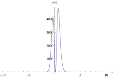
Figure 1: Graph of $\rho=|\Phi|^{2}$ for the parameters: $\alpha=2;n=1;\omega=3;\delta=10;\epsilon=5$.

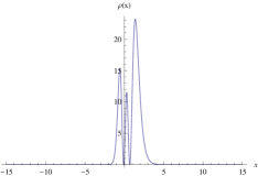
Figure 2: Graph of $\rho=|\Phi|^{2}$ for the parameters: $\alpha=2;n=2;\omega=3;\delta=10;\epsilon=4$.

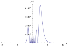
Figure 3: Graph of $\rho=|\Phi|^{2}$ for the parameters: $\alpha=2;n=8;\omega=3;\delta=10;\epsilon=4$.

References

- [1] C. M. Bender and S. Boettcher, Phys. Rev. Lett. 80 5243 1998.
- [2] For a review, see C. M. Bender Rep. Prog. Phys. 70 947 2007.
- [3] C. M. Bender and H. F. Jones, Phys. Rev. A 85 052118 2012.
- [4] C. M. Bender, Czec. J. Phys. 54 1027 2004.
- [5] C. M. Bender, D. C. Brody and H. F. Jones Phys. Rev. Lett. 89 270401 2002; 92 119902 2002.
- [6] Bender C M, Brody D C and Jones H F Phys. Rev. D 70 025001 2004; 71 049901 2004.
- [7] A. Arda, R. Sever, Phys. Scr. 82 065007 2010.
- [8] Y. N. Joglekar, B. Bagchi, J. Phys. A: Math. Theo. 45 402001 2012.
- [9] Ö. Yeşiltaş, Phys. Scr. 2007 75 41.
- [10] K. Saaidi, E. Karimi, K. Heshami and P. Seifpanahi Phys. Scr. 77 065002 2008.
- [11] Christian E. Rutter et al, Nature Physics 6 192 2010.
- [12] K. G. Makris et al, Physical Review A 81 063807 2010.
- [13] A. Guo et al, Phys. Rev. Lett. 103 093902 2009.
- [14] A. Mostafazadeh, J. Math. Phys. 43 205 2002; J. Math. Phys. 43 2814 2002; J. Math. Phys. 43 3944 2002.
- [15] F G Scholtz, H B Geyer and F J W Hahne, Ann. Phys. NY 213 74 1992; R Kretschmer and L Szymanowski, Phys. Lett. A 325 112 2004.
- [16] R. Roychoudhury, B. Roy, Phys. Lett. A 361(4-5) 291 2007.
- [17] R. Roychoudhury, B. Roy, Phys. Lett. A 372(7) 997 2008.
- [18] A. Sinha, P. Roy, J. Math. Phys. 46 032102 2005.
- [19] Ö. Yeşiltaş J. Phys. A: Math. Theor. 44 305305 2011.
- [20] M. S. Swanson J. Math. Phys. 45 585 2004.
- [21] Paulo E G Assis, J. Phys. A: Math. Theor. 44 265303 2011.
- [22] D P Musumbu, H B Geyer, W D Heiss, J. Phys. A: Math. Theor. 40 F75 2007.
- [23] C. Quesne, J. Phys. A 41 244022 2008.
- [24] B. Bagchi, C. Quesne and R. Roychoudhury, J. Phys. A 38 L647 2005.
- [25] B. Midya, P P Dube and R. Roychoudhury, J. Phys. A: Math. Theo. 44(6) 062001 2011.
- [26] A. Sinha and P. Roy, J. Phys. A: Math. Theor. 40 10599 2007; J. Phys. A: Math. Theor. 41 335306 2008.
- [27] Ö. Yeşiltaş, PT Symmetric Hamiltonian Model and Exactly Solvable Potentials, International Conference on Mathematical Modeling in Physical Sciences September 3-7, 2012 Budapest, Hungary IOP Publishing, Journal of Physics: Conference Series, 410 012076 2013.
- [28] Ö. Yeşiltaş J. Phys. A: Math. Theor. 46 015302 2013.
- [29] F. Cooper, A. Khare U. Sukhatme, Supersymmetry in Quantum Mechanics, World Sci. Pub. Co. Pte. Ltd. 2001 ISBN: 981-02-4605-6.
- [30] G. Lévai and E. Magyari, J. Phys. A: Math. Theor. 42 195302 2009.