Fermionic two-loop functional renormalization group for correlated fermions: Method and application to the attractive Hubbard model

Abstract

We derive an efficient method for treating renormalization contributions at two-loop level within the functional renormalization group in the one-particle irreducible formalism for fermions. It is based on a decomposition of the two-particle vertex in charge, magnetic and pairing channels. The method treats single-particle and collective excitations in all channels on equal footing, allows for the description of symmetry-breaking and captures collective mode fluctuation physics in the infrared. As a first application, we study the superfluid ground state of the two-dimensional attractive Hubbard model. We obtain superfluid gaps that are reduced by fluctuations in comparison to the one-loop approximation and demonstrate that the method captures the renormalization of the amplitude mode by long-range phase fluctuations.

I Introduction

In the last decade, the functional renormalization group (fRG) proved itself as an excellent tool for the study of competing instabilities in correlated electron systems and a valuable source of new approximation schemes.*[Forareview; see]Metzner2012 It treats charge, magnetic and pairing channels on equal footing and in a scale-separated way. This allows for the study of competing order and fluctuation driven instabilities. One of the major successes of fRG was to provide evidence for $d$-wave superconductivity in the two-dimensional repulsive Hubbard model at weak and intermediate couplings.Zanchi and Schulz (2000); Halboth and Metzner (2000); Honerkamp et al. (2001); Eberlein and Metzner (2014) The method was also successfully applied to quantum wires and dots in and out of equilibrium,Andergassen et al. (2004); Karrasch et al. (2010) multiband systems describing pnictide superconductors Wang et al. (2009); Thomale et al. (2009); Platt et al. (2009) and also spin models.Reuther and Wölfle (2010); Reuther and Thomale (2011)

Most of these fRG studies used the one-particle irreducible (1PI) formalism in a purely fermionic formulation and were restricted to the one-loop level without or with taking the self-energy feedback into account in the flow equation for the vertex as suggested by Katanin.Katanin (2004) The latter modification improves the fulfillment of Ward identities and allows to continue fermionic fRG flows into phases with broken symmetries.Salmhofer et al. (2004); Gersch et al. (2005, 2008); Maier and Honerkamp (2012); Eberlein and Metzner (2013, 2014); Maier et al. (2014) However, in a recent study of superfluidity in the attractive Hubbard model, it was pointed out that the singular infrared behavior of the amplitude mode of the gap due to phase fluctuations Castellani et al. (1997); Pistolesi et al. (2004) is not captured in the Katanin scheme.Eberlein and Metzner (2013); Eberlein (2013)

An alternative route to studying fluctuation physics and symmetry breaking is to decouple the fermionic fields by introducing bosonic auxiliary fields via a Hubbard-Stratonovich transformation. Applying the fRG to the resulting mixed fermion-boson action captures the asymptotic infrared behavior of fermionic superfluids already at one-loop level within a relatively simple truncation.Strack et al. (2008); Obert et al. (2013) Besides fermionic superfluidity,Birse et al. (2005); Strack et al. (2008); Obert et al. (2013) this route was also pursued for studying the BEC-BCS crossover in continuum systems,Diehl et al. (2007); Bartosch et al. (2009); Diehl et al. (2010) and antiferromagnetism Baier et al. (2004) as well as $d$-wave superconductivity Friederich et al. (2011) in the two-dimensional Hubbard model.

The choice of auxiliary fields introduces some bias if only a small number of them and simple truncations are used.Baier et al. (2004) This bias can be reduced by dynamical rebosonization.Gies and Wetterich (2002); Floerchinger and Wetterich (2009) Most fRG studies of partially bosonized actions relied on relatively simple ansätze for the bosonic potential. However, in situations with competition of instabilities, truncating the order parameter potential is not straightforward. It may therefore be advantageous to treat at least the high and intermediate scales in a purely fermionic language. In addition, results for the vertex in the Hubbard model at large couplings indicate that the effective interaction contains contributions that are not well described as boson-mediated interactions.Rohringer et al. (2012); Kinza and Honerkamp (2013) Recently, Veschgini and Salmhofer derived a hierarchy of flow equations for fermionic 1PI vertex functions from Dyson-Schwinger equations and pointed out that including all renormalization contributions at two-loop level may increase the degree of self-consistency.Veschgini and Salmhofer (2013)

All this motivates going beyond the one-loop approximation or Katanin’s scheme within the purely fermionic formalism. One fRG study at two-loop level has been carried out for the repulsive Hubbard model in the symmetric regime by Katanin.Katanin (2009) He used the $N$-patch approximation for the momentum dependence of the vertex and neglected its frequency dependence. For relatively weak couplings, he concluded that fluctuations at two-loop level do not change the flow qualitatively. This is not clear at larger couplings and in symmetry-broken phases. Besides, in such situations the frequency dependence of the vertex should be taken into account, which seems to be beyond the scope of Katanin’s two-loop approach due to the resulting numerical complexity.

In this article, we present a reformulation of the two-loop flow equations that is effectively of one-loop form. It is exact to the third order in the effective interaction and based on a decomposition of the vertex in charge, magnetic and pairing channels.Karrasch et al. (2008); Husemann and Salmhofer (2009) It allows to take the frequency dependence of the vertex into account with a reasonable numerical effort and to continue fRG flows into symmetry-broken phases. We demonstrate that the method captures the singular asymptotic infrared behavior of a fermionic $s$-wave superfluid. Besides the general scheme, we present as a first application a study of the superfluid ground state of the attractive Hubbard model. In the presence of a not too small external pairing field, the one- and two-loop flows are qualitatively similar, albeit with smaller critical scales and gaps at two-loop level. The infrared behavior is different in the two approximations, as expected.

The article is structured as follows. In Sec. II, we describe the reformulated flow equations at two-loop level that allow for an efficient numerical solution. In Sec. III, results for the attractive Hubbard model are presented, including estimates for the infrared behavior and numerical results. Section IV contains a short summary and final remarks.

II Method

In this section, we describe the reformulation of the two-loop flow equations as effective one-loop equations, which is at the heart of this article. The result is applicable to all systems whose effective actions contain vertices with an equal number of creation and annihilation operators only (see below) and in which it is meaningful to classify diagrams according to singular dependences on transfer momenta or frequencies.

A general derivation of renormalization group equations in the 1PI framework can be found for example in Ref. Metzner et al., 2012. Flow equations at two-loop level were derived for example in Refs. Salmhofer et al., 2004; Veschgini and Salmhofer, 2013.

II.1 Flow equations at two-loop level

In this section, we outline the derivation of flow equations at two-loop level in order to make the article self-contained, following the presentations in Refs. Salmhofer et al., 2004; Eberlein, 2013.

Flow equations at two-loop level are based on a truncation of the flowing effective action $\Gamma^{\Lambda}[\bar{\phi},\phi]$ at the three-particle level,

$$\begin{split}\Gamma^{\Lambda}&[\bar{\phi},\phi]=\Gamma^{(0)\Lambda}+\sum_{\alpha,\beta}\Gamma^{(2)\Lambda}_{\alpha\beta}\bar{\phi}_{\alpha}\phi_{\beta}\\ &+\frac{1}{4}\sum_{\alpha,\beta,\gamma,\delta}\Gamma^{(4)\Lambda}_{\alpha\beta\gamma\delta}\bar{\phi}_{\alpha}\bar{\phi}_{\beta}\phi_{\gamma}\phi_{\delta}\\ &+\frac{1}{(3!)^{2}}\sum_{\alpha,\beta,\gamma,\delta,\epsilon,\zeta}\Gamma^{(6)\Lambda}_{\alpha\beta\gamma\delta\epsilon\zeta}\bar{\phi}_{\alpha}\bar{\phi}_{\beta}\bar{\phi}_{\gamma}\phi_{\delta}\phi_{\epsilon}\phi_{\zeta}+\ldots,\end{split}$$ (1)

where $\bar{\phi}$, $\phi$ are anticommuting Grassmann fields and $\Gamma^{(2n)\Lambda}$ the 1PI $n$-particle vertex functions. The ellipsis represents four-particle and higher-order terms. The Greek indices $\alpha=(k,s)$, with $k=(k_{0},\boldsymbol{k})$, collect momenta $\boldsymbol{k}$ as well as fermionic Matsubara frequencies $k_{0}$ and the spin or Nambu index $s$. For describing a system in the symmetric phase, the fermionic fields can be chosen in spinor representation, $\phi_{\alpha}\rightarrow\psi_{ks}$ and $\bar{\phi}_{\alpha}\rightarrow\bar{\psi}_{ks}$, where $s=\uparrow\downarrow$ is the spin orientation. For a fermionic singlet superfluid or superconductor, as considered in the following, the fields are most conveniently chosen in Nambu representation, where $s=\pm$ is the Nambu index and

$$\phi_{k+}=\psi_{k\uparrow},\quad\bar{\phi}_{k+}=\bar{\psi}_{k\uparrow},\quad\phi_{k-}=\bar{\psi}_{-k\downarrow},\quad\bar{\phi}_{k-}=\psi_{-k\downarrow}.$$ (2)

Using this representation in the presence of spin rotation invariance, only vertices that create and annihilate an equal number of Nambu quasiparticles appear in the effective action.Gersch et al. (2008); Eberlein and Metzner (2010)

Inserting the ansatz for the effective action Eq. (1) into the functional flow equation and evaluating appropriate functional derivatives with respect to the fields (see Ref. Metzner et al., 2012) yields flow equations for the self-energy

$$\frac{d}{d\Lambda}\Sigma^{\Lambda}_{\alpha\beta}=\sum_{\gamma,\delta}S^{\Lambda}_{\delta\gamma}\Gamma^{(4)\Lambda}_{\alpha\gamma\delta\beta}$$ (3)

and the two-particle vertex

$$\begin{split}\frac{d}{d\Lambda}&\Gamma^{(4)\Lambda}_{\alpha\beta\gamma\delta}=\\ &\sum_{a,b,c,d}\Bigr{[}\partial_{\Lambda,S}(G^{\Lambda}_{ab}G^{\Lambda}_{cd})(\Gamma^{(4)\Lambda}_{\alpha bc\delta}\Gamma^{(4)\Lambda}_{d\beta\gamma a}-\Gamma^{(4)\Lambda}_{\beta bc\delta}\Gamma^{(4)\Lambda}_{d\alpha\gamma a})\\ &-\frac{1}{2}\partial_{\Lambda,S}(G^{\Lambda}_{ab}G^{\Lambda}_{cd})\Gamma^{(4)\Lambda}_{\alpha\beta ca}\Gamma^{(4)\Lambda}_{bd\gamma\delta}\Bigr{]}+\sum_{a,b}S^{\Lambda}_{ba}\Gamma^{(6)\Lambda}_{\alpha\beta ab\gamma\delta},\end{split}$$ (4)

where $G^{\Lambda}_{\alpha\beta}=(\Gamma^{(2)\Lambda})^{-1}_{\alpha\beta}$ is the full fermionic propagator and $S^{\Lambda}_{\alpha\beta}=(\frac{d}{d\Lambda}G^{\Lambda}_{\alpha\beta})_{\Sigma^{\Lambda}=\text{const.}}\equiv\partial_{\Lambda,S}G^{\Lambda}_{\alpha\beta}$ the so-called single-scale propagator. The self-energy is connected to $\Gamma^{(2)\Lambda}$ via a Dyson-Schwinger equation, $(G^{\Lambda})^{-1}_{\alpha\beta}=(G^{\Lambda}_{0})^{-1}_{\alpha\beta}-\Sigma^{\Lambda}_{\alpha\beta}$, where $G^{\Lambda}_{0}$ is the regularized bare propagator at scale $\Lambda$. The flow equation for the two-particle vertex is illustrated diagrammatically in Fig. 1.

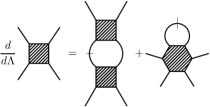
Figure 1: Simplified diagrammatic representation of the one-loop renormalization group equation for the two-particle vertex.

Figure 2: Simplified diagrammatic representation of the one-loop renormalization group equation for the three-particle vertex.

The flow equation for the three-particle vertex can be written schematically as

$$\begin{split}\frac{d}{d\Lambda}\Gamma^{(6)\Lambda}=&\Gamma^{(4)\Lambda}\partial_{\Lambda,S}(G^{\Lambda}G^{\Lambda})\Gamma^{(6)\Lambda}+S^{\Lambda}\Gamma^{(8)\Lambda}\\ &+\partial_{\Lambda,S}\operatorname{tr}(G^{\Lambda}\Gamma^{(4)\Lambda}G^{\Lambda}\Gamma^{(4)\Lambda}G^{\Lambda}\Gamma^{(4)\Lambda})\end{split}$$ (5)

and is illustrated diagrammatically in Fig. 2. A solution for $\Gamma^{(6)\Lambda}$ in $\mathcal{O}((\Gamma^{(4)\Lambda})^{3})$ is obtained by neglecting the contributions in the first line of Eq. (5), because these are at least of fourth order in the effective interaction. At the same level of approximation, the scale-derivative $\partial_{\Lambda,S}$ in the second line of Eq. (5) can be replaced by a full scale-derivative $\frac{d}{d\Lambda}$ that acts also on the self-energy and the vertex. The latter modification generates terms at least of $\mathcal{O}((\Gamma^{(4)\Lambda})^{4})$. The resulting flow equation Salmhofer et al. (2004)

$$\frac{d}{d\Lambda}\Gamma^{(6)\Lambda}=\frac{d}{d\Lambda}\operatorname{tr}(G^{\Lambda}\Gamma^{(4)\Lambda}G^{\Lambda}\Gamma^{(4)\Lambda}G^{\Lambda}\Gamma^{(4)\Lambda})$$ (6)

can straightforwardly be integrated because the right hand side is a total derivative, yielding

$$\Gamma^{(6)\Lambda}=\operatorname{tr}(G^{\Lambda}\Gamma^{(4)\Lambda}G^{\Lambda}\Gamma^{(4)\Lambda}G^{\Lambda}\Gamma^{(4)\Lambda})$$ (7)

in a system with only two-particle interactions at the microscopic level. In more detail, the three-particle vertex in $\mathcal{O}((\Gamma^{(4)\Lambda})^{3})$ reads

$$\Gamma^{(6)\Lambda}_{\alpha\beta ab\gamma\delta}=(\Gamma^{(6)\Lambda}_{\alpha\beta ab\gamma\delta})_{(1)}+(\Gamma^{(6)\Lambda}_{\alpha\beta ab\gamma\delta})_{(2)},$$ (8)

$$\begin{split}(\Gamma^{(6)\Lambda}_{\alpha\beta ab\gamma\delta})_{(1)}=-\sum_{c,d,e,f,m,n}&G^{\Lambda}_{cd}G^{\Lambda}_{ef}G^{\Lambda}_{mn}\bigl{(}\Gamma^{(4)\Lambda}_{\alpha ne\delta}\Gamma^{(4)\Lambda}_{\beta dmb}\Gamma^{(4)\Lambda}_{afc\gamma}-\Gamma^{(4)\Lambda}_{\alpha ne\delta}\Gamma^{(4)\Lambda}_{admb}\Gamma^{(4)\Lambda}_{\beta fc\gamma}+\Gamma^{(4)\Lambda}_{\alpha ne\gamma}\Gamma^{(4)\Lambda}_{admb}\Gamma^{(4)\Lambda}_{\beta fc\delta}-\Gamma^{(4)\Lambda}_{\alpha ne\gamma}\Gamma^{(4)\Lambda}_{\beta dmb}\Gamma^{(4)\Lambda}_{afc\delta}\\[-8.61108pt] &\hskip 40.00006pt+\Gamma^{(4)\Lambda}_{\alpha ne\delta}\Gamma^{(4)\Lambda}_{adm\gamma}\Gamma^{(4)\Lambda}_{\beta fcb}-\Gamma^{(4)\Lambda}_{\alpha ne\delta}\Gamma^{(4)\Lambda}_{\beta dm\gamma}\Gamma^{(4)\Lambda}_{afcb}-\Gamma^{(4)\Lambda}_{\alpha ne\gamma}\Gamma^{(4)\Lambda}_{adm\delta}\Gamma^{(4)\Lambda}_{\beta fcb}+\Gamma^{(4)\Lambda}_{\alpha ne\gamma}\Gamma^{(4)\Lambda}_{\beta dm\delta}\Gamma^{(4)\Lambda}_{afcb}\\ &\hskip 40.00006pt-\Gamma^{(4)\Lambda}_{\alpha neb}\Gamma^{(4)\Lambda}_{adm\gamma}\Gamma^{(4)\Lambda}_{\beta fc\delta}+\Gamma^{(4)\Lambda}_{\alpha neb}\Gamma^{(4)\Lambda}_{\beta dm\gamma}\Gamma^{(4)\Lambda}_{afc\delta}+\Gamma^{(4)\Lambda}_{\alpha neb}\Gamma^{(4)\Lambda}_{adm\delta}\Gamma^{(4)\Lambda}_{\beta fc\gamma}-\Gamma^{(4)\Lambda}_{\alpha neb}\Gamma^{(4)\Lambda}_{\beta dm\delta}\Gamma^{(4)\Lambda}_{afc\gamma}\bigr{)},\end{split}$$ (9)

$$\begin{split}(\Gamma^{(6)\Lambda}_{\alpha\beta ab\gamma\delta})_{(2)}=-\sum_{c,d,e,f,m,n}&G^{\Lambda}_{cd}G^{\Lambda}_{ef}G^{\Lambda}_{mn}\bigl{(}\Gamma^{(4)\Lambda}_{\beta acm}\Gamma^{(4)\Lambda}_{fd\gamma\delta}\Gamma^{(4)\Lambda}_{\alpha neb}+\Gamma^{(4)\Lambda}_{a\alpha cm}\Gamma^{(4)\Lambda}_{fd\gamma\delta}\Gamma^{(4)\Lambda}_{\beta neb}+\Gamma^{(4)\Lambda}_{\alpha\beta cm}\Gamma^{(4)\Lambda}_{fd\gamma\delta}\Gamma^{(4)\Lambda}_{aneb}+\Gamma^{(4)\Lambda}_{\alpha\beta cm}\Gamma^{(4)\Lambda}_{fdb\gamma}\Gamma^{(4)\Lambda}_{ane\delta}\\[-8.61108pt] &\hskip 40.00006pt+\Gamma^{(4)\Lambda}_{\alpha\beta cm}\Gamma^{(4)\Lambda}_{fd\delta b}\Gamma^{(4)\Lambda}_{ane\gamma}+\Gamma^{(4)\Lambda}_{\beta acm}\Gamma^{(4)\Lambda}_{fdb\gamma}\Gamma^{(4)\Lambda}_{\alpha ne\delta}+\Gamma^{(4)\Lambda}_{\beta acm}\Gamma^{(4)\Lambda}_{fd\delta b}\Gamma^{(4)\Lambda}_{\alpha ne\gamma}+\Gamma^{(4)\Lambda}_{a\alpha cm}\Gamma^{(4)\Lambda}_{fdb\gamma}\Gamma^{(4)\Lambda}_{\beta ne\delta}\\ &\hskip 40.00006pt+\Gamma^{(4)\Lambda}_{a\alpha cm}\Gamma^{(4)\Lambda}_{fd\delta b}\Gamma^{(4)\Lambda}_{\beta be\gamma}\bigr{)}.\end{split}$$ (10)

In Eq. (9) all internal propagators run into the same direction, while this is not the case in Eq. (10). Inserting these expressions in Eq. (4) yields the flow equation for the two-particle vertex at two-loop level, which is illustrated schematically in Fig. 3.

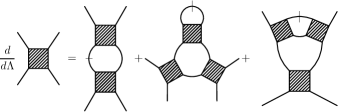
Figure 3: Simplified diagrammatic representation of the two-loop flow equation for the two-particle vertex. The second and third diagrams on the right hand side can be classified as two-loop contributions with non-overlapping and overlapping loops, respectively.

The two-loop diagrams can be classified in contributions with non-overlapping and overlapping loops, which have the topological structure of the second and third diagram on the right hand side of Fig. 3, respectively. In two-loop diagrams with non-overlapping loops, the single-scale propagator in Eq. (4) contracts two indices at the same vertex. As discussed by Katanin,Katanin (2004) these contributions can be rewritten as one-loop diagrams with an insertion of $\dot{\Sigma}^{\Lambda}$. Exploiting the relation $\dot{G}^{\Lambda}=S^{\Lambda}+G^{\Lambda}\dot{\Sigma}^{\Lambda}G^{\Lambda}$, they allow to replace the single-scale propagators in the one-loop contributions in Eq. (4) by scale-differentiated full propagators.

The two-loop contributions with overlapping loops can be treated in a similar fashion after decomposing the vertex in interaction channels, which is discussed in the next section.

II.2 Channel-decomposed flow equations at two-loop level: $\boldsymbol{\dot{\Gamma}}$ scheme

In this section, we discuss how the two-loop contributions with overlapping loops can be reformulated effectively as one-loop contributions, and derive a channel-decomposition scheme for the vertex and the flow equations at two-loop level. The latter allows to extend the one-loop schemes by Karrasch et al. Karrasch et al. (2008) and Husemann and Salmhofer Husemann and Salmhofer (2009) for the symmetric phase, by the author and Metzner for singlet superconductors,Eberlein and Metzner (2010) and by Maier and Honerkamp for antiferromagnets.Maier and Honerkamp (2012)

The basic idea is to rewrite the insertions of two vertices that are connected by a full and a single-scale propagator in the two-loop contributions with overlapping loops (see third diagram on the right hand side of Fig. 3) as one-loop contribution (see first diagram on right hand side of Fig. 3). In order to make use of this idea, the vertex has to be decomposed in interaction channels and the diagrams in the flow equation have to be assigned to channels according to their leading singular dependence on external momenta and frequencies.

For a decomposition in interaction channels, the two-particle vertex is written as a sum of several terms, where each describes a possibly singular dependence of the vertex on momenta and frequencies. Assuming translation invariance, the multiindex notation of section II.1 is specialized to

$$\Gamma^{(4)\Lambda}_{\alpha\beta\gamma\delta}\equiv\Gamma^{(4)\Lambda}_{s_{\alpha}s_{\beta}s_{\gamma}s_{\delta}}(k_{\alpha},k_{\beta},k_{\gamma},k_{\delta}),$$ (11)

where $\Gamma^{(4)\Lambda}$ is nonzero only for $k_{\alpha}+k_{\beta}=k_{\gamma}+k_{\delta}$. For the sake of compactness of the presentation, we stick to the multiindex notation in the major part of this section. The channel-decomposition of the vertex reads

$$\begin{split}\Gamma^{(4)\Lambda}_{\alpha\beta\gamma\delta}&=u_{\alpha\beta\gamma\delta}+V^{\text{PH},\Lambda}_{\alpha\beta\gamma\delta}-V^{\text{PH},\Lambda}_{\beta\alpha\gamma\delta}+V^{\text{PP},\Lambda}_{\alpha\beta\gamma\delta},\end{split}$$ (12)

where $u$ is the microscopic interaction and

$$V^{\text{PH},\Lambda}_{\alpha\beta\gamma\delta}=V^{\text{PH},\Lambda}_{s_{\alpha}s_{\beta}s_{\gamma}s_{\delta}}\bigl{(}k_{\gamma}-k_{\beta};\tfrac{k_{\alpha}+k_{\delta}}{2},\tfrac{k_{\beta}+k_{\gamma}}{2}\bigr{)},$$ (13)

$$V^{\text{PP},\Lambda}_{\alpha\beta\gamma\delta}=V^{\text{PP},\Lambda}_{s_{\alpha}s_{\beta}s_{\gamma}s_{\delta}}\bigl{(}k_{\alpha}+k_{\beta};\tfrac{k_{\alpha}-k_{\beta}}{2},\tfrac{k_{\delta}-k_{\gamma}}{2}\bigr{)}$$ (14)

describe fluctuation corrections in the (Nambu) particle-hole and (Nambu) particle-particle channel, respectively. The first argument of $V^{\text{PH},\Lambda}$ and $V^{\text{PP},\Lambda}$ describes the possibly singular dependence on the transfer momentum, while the last two momentum arguments describe dependences on fermionic relative momenta. The decomposition of the vertex is illustrated diagrammatically in Fig. 4.

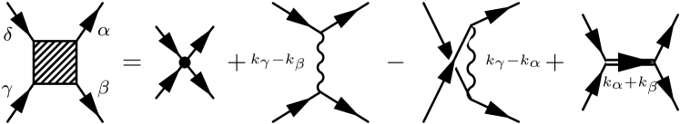
Figure 4: Diagrammatic representation of the decomposition of the (Nambu) two-particle vertex in bare interaction, particle-hole channels and particle-particle channel.

Flow equations for the effective interactions in the particle-hole and particle-particle channels are derived by inserting the ansatz Eq. (12) into the flow equation (4) and assigning diagrams to interaction channels according to their leading singular dependence on external momenta. The one-loop contributions (i. e., Eq. (4) without the last term) are assigned to interaction channels as in the channel-decomposition schemes at one-loop level in such a way that the transfer momentum is transported through the diagrams by the fermionic propagators. The first and second contributions in the square bracket in Eq. (4) are assigned to the direct and crossed particle-hole channel, respectively. The third contribution is assigned to the particle-particle channel. This yields

$$\begin{split}\bigl{(}\frac{d}{d\Lambda}V^{\text{PH},\Lambda}_{\alpha\beta\gamma\delta}\bigr{)}_{\text{1L}}&=\sum_{a,b,c,d}\partial_{\Lambda,S}(G^{\Lambda}_{ab}G^{\Lambda}_{cd})\Gamma^{(4)\Lambda}_{\alpha bc\delta}\Gamma^{(4)\Lambda}_{d\beta\gamma a}\\ &\equiv\dot{V}^{\text{PH},\Lambda}_{\alpha\beta\gamma\delta},\end{split}$$ (15)

$$\begin{split}\bigl{(}\frac{d}{d\Lambda}V^{\text{PP},\Lambda}_{\alpha\beta\gamma\delta}\bigr{)}_{\text{1L}}&=-\frac{1}{2}\sum_{a,b,c,d}\partial_{\Lambda,S}(G^{\Lambda}_{ab}G^{\Lambda}_{cd})\Gamma^{(4)\Lambda}_{\alpha\beta ca}\Gamma^{(4)\Lambda}_{bd\gamma\delta}\\ &\equiv\dot{V}^{\text{PP},\Lambda}_{\alpha\beta\gamma\delta}\end{split}$$ (16)

After rewriting the two-loop diagrams with non-overlapping loops as one-loop diagrams with $\dot{\Sigma}$-insertions, they are assigned similarly according to the transfer momentum in the fermionic loops,

$$\bigl{(}\frac{d}{d\Lambda}V^{\text{PH},\Lambda}_{\alpha\beta\gamma\delta}\bigr{)}_{\dot{\Sigma}}=\sum_{a,b,c,d}\partial_{\Lambda,\Sigma}(G^{\Lambda}_{ab}G^{\Lambda}_{cd})\Gamma^{(4)\Lambda}_{\alpha bc\delta}\Gamma^{(4)\Lambda}_{d\beta\gamma a},$$ (17)

$$\bigl{(}\frac{d}{d\Lambda}V^{\text{PP},\Lambda}_{\alpha\beta\gamma\delta}\bigr{)}_{\dot{\Sigma}}=-\frac{1}{2}\sum_{a,b,c,d}\partial_{\Lambda,\Sigma}(G^{\Lambda}_{ab}G^{\Lambda}_{cd})\Gamma^{(4)\Lambda}_{\alpha\beta ca}\Gamma^{(4)\Lambda}_{bd\gamma\delta},$$ (18)

where $\partial_{\Lambda,\Sigma}$ is a shorthand for a $\Lambda$-derivative that acts on the fermionic self-energy only, $\partial_{\Lambda,\Sigma}G^{\Lambda}=G^{\Lambda}\dot{\Sigma}^{\Lambda}G^{\Lambda}$.

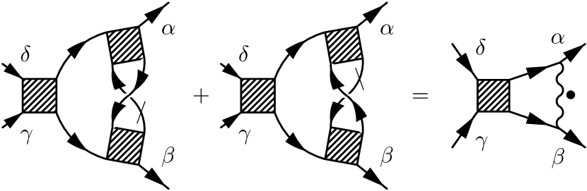
Figure 5: Illustration of the reorganization of two-loop diagrams with overlapping loops in a one-loop diagram with a scale-differentiated effective interaction.

Before assigning the two-loop contributions with overlapping loops to the interaction channels, it is convenient to rewrite them effectively as one-loop diagrams. This is possible after expressing insertions of two vertices that are connected by a full and a single-scale propagator as one-loop scale-derivatives of effective interactions. Consider as an example the renormalization contribution to the two-particle vertex arising from the first two terms in the first line of Eq. (10). After insertion into Eq. (4), these contributions read

$$-\sum S^{\Lambda}_{ba}G^{\Lambda}_{cd}G^{\Lambda}_{ef}G^{\Lambda}_{mn}(\Gamma^{(4)\Lambda}_{\beta acm}\Gamma^{(4)\Lambda}_{\alpha neb}+\Gamma^{(4)\Lambda}_{a\alpha cm}\Gamma^{(4)\Lambda}_{\beta neb})\Gamma^{(4)\Lambda}_{fd\gamma\delta}.$$ (19)

Renaming summation indices and exploiting the antisymmetry of the vertex under particle exchange, this expression can be rewritten as

$$-\sum\Gamma^{(4)\Lambda}_{fd\gamma\delta}G^{\Lambda}_{ef}G^{\Lambda}_{cd}\underbrace{(S^{\Lambda}_{ba}G^{\Lambda}_{mn}+G^{\Lambda}_{ba}S^{\Lambda}_{mn})\Gamma^{(4)\Lambda}_{\alpha nbe}\Gamma^{(4)\Lambda}_{a\beta cm}}_{=\bigl{(}\frac{d}{d\Lambda}V^{\text{PH},\Lambda}_{\alpha\beta ce}\bigr{)}_{\text{1L}}}$$

$$=-\sum_{c,d,e,f}\bigl{(}\frac{d}{d\Lambda}V^{\text{PH},\Lambda}_{\alpha\beta ce}\bigr{)}_{\text{1L}}G^{\Lambda}_{ef}G^{\Lambda}_{cd}\Gamma^{(4)\Lambda}_{fd\gamma\delta},$$ (20)

where Eq. (15) was exploited. This reorganization is illustrated diagrammatically in Fig. 5 and works similarly for all contributions in Eq. (4) after inserting Eqs. (9) and (10). Collecting terms yields the two-loop flow equation for the vertex expressed effectively as a one-loop equation,

$$\begin{split}\frac{d}{d\Lambda}\Gamma^{(4)\Lambda}_{\alpha\beta\gamma\delta}&=\sum_{a,b,c,d}\Bigr{[}\frac{d}{d\Lambda}(G^{\Lambda}_{ab}G^{\Lambda}_{cd})(\Gamma^{(4)\Lambda}_{\alpha bc\delta}\Gamma^{(4)\Lambda}_{d\beta\gamma a}-\Gamma^{(4)\Lambda}_{\beta bc\delta}\Gamma^{(4)\Lambda}_{d\alpha\gamma a})-\frac{1}{2}\frac{d}{d\Lambda}(G^{\Lambda}_{ab}G^{\Lambda}_{cd})\Gamma^{(4)\Lambda}_{\alpha\beta ca}\Gamma^{(4)\Lambda}_{bd\gamma\delta}\Bigr{]}\\ &+\sum_{a,b,c,d}G^{\Lambda}_{ab}G^{\Lambda}_{cd}\Bigl{[}\Gamma^{(4)\Lambda}_{\alpha bc\delta}\dot{V}^{\text{PP},\Lambda}_{\beta da\gamma}-\Gamma^{(4)\Lambda}_{\alpha bc\gamma}\dot{V}^{\text{PP},\Lambda}_{\beta da\delta}+\dot{V}^{\text{PP},\Lambda}_{\alpha bc\delta}\Gamma^{(4)\Lambda}_{\beta da\gamma}-\dot{V}^{\text{PP},\Lambda}_{\alpha bc\gamma}\Gamma^{(4)\Lambda}_{\beta da\delta}-\Gamma^{(4)\Lambda}_{\alpha bc\delta}\dot{V}^{\text{PH},\Lambda}_{\beta d\gamma a}\\ &\hskip 50.00008pt+\Gamma^{(4)\Lambda}_{\alpha bc\gamma}\dot{V}^{\text{PH},\Lambda}_{\beta d\delta a}+\dot{V}^{\text{PH},\Lambda}_{\alpha d\gamma a}\Gamma^{(4)\Lambda}_{\beta bc\delta}-\dot{V}^{\text{PH},\Lambda}_{\alpha d\delta a}\Gamma^{(4)\Lambda}_{\beta bc\gamma}-\Gamma^{(4)\Lambda}_{\alpha\beta ca}\dot{V}^{\text{PH},\Lambda}_{bd\gamma\delta}-\dot{V}^{\text{PH},\Lambda}_{\alpha\beta ca}\Gamma^{(4)\Lambda}_{bd\gamma\delta}\Bigr{]}.\end{split}$$ (21)

Figure 6: Examples for (a) vertex correction and (b,c) box diagrams. At two-loop level, the scale-derivative acts on the effective interactions that transport the loop momentum $p$. The transfer momentum is transported through the diagram by the fermionic propagators in (a) and (b), while it is transported by the effective interactions in (c).

In order to make use of this reorganization, we insert the decomposition of the vertex in interaction channels Eq. (12) on both sides of Eq. (21) and assign diagrams to interaction channels according to their leading singular dependence on external momenta. The assignment of the contributions in the first line of Eq. (21) was discussed above. After inserting the decomposition of the vertex, the second and third lines contain diagrams that can be classified in two-loop vertex correction diagrams (for an example see Fig. 6) and two-loop box diagrams (for examples see Figs. 6 and 6). No two-loop propagator renormalization diagrams appear as a consequence of the topological structure of the two-loop diagrams with overlapping loops.

Like at one-loop level, the vertex correction diagrams are assigned to interaction channels according to the transfer momentum in the fermionic loop and in one effective interaction. The singular dependence on momentum in the other effective interaction is integrated and does not give rise to singular renormalization contributions in the ground state of a fermionic $s$-wave superfluid (see section III.2). Differently from one-loop level, the two-loop box diagrams are assigned to interaction channels in such a way that the transfer momentum is transported through the diagram by the effective interactions (as shown in the example in Fig. 6). The reason is that these diagrams become important close to and below the critical scale,Salmhofer and Honerkamp (2001) where the effective interactions and their scale-derivatives already developed a strong dependence on momentum and frequency. The assignment according to the “bosonic” singularity yields a better treatment of the strong momentum and frequency dependence of the scale-differentiated effective interactions. In section III.2, we demonstrate that this assignment allows to capture the singular renormalization of the amplitude mode by long-range phase fluctuations in a fermionic $s$-wave superfluid. The two-loop renormalization contributions to the effective interaction in the (Nambu) particle-hole and particle-particle channels read

$$\begin{split}\bigl{(}\frac{d}{d\Lambda}V^{\text{PH},\Lambda}_{\alpha\beta\gamma\delta}\bigr{)}_{\text{2L}}=\sum_{a,b,c,d}G^{\Lambda}_{ab}G^{\Lambda}_{cd}&\Bigl{[}\bigl{(}u_{\alpha bc\delta}+V^{\text{PH},\Lambda}_{\alpha bc\delta}\bigr{)}\bigl{(}\dot{V}^{\text{PP},\Lambda}_{d\beta\gamma a}-\dot{V}^{\text{PH},\Lambda}_{\beta d\gamma a}\bigr{)}+\bigl{(}\dot{V}^{\text{PP},\Lambda}_{\alpha bc\delta}-\dot{V}^{\text{PH},\Lambda}_{b\alpha c\delta}\bigr{)}\bigl{(}u_{d\beta\gamma a}+V^{\text{PH},\Lambda}_{d\beta\gamma a}\bigr{)}\\ &-\frac{d}{d\Lambda}\bigl{(}V^{\text{PP},\Lambda}_{\alpha bc\gamma}V^{\text{PP},\Lambda}_{d\beta\delta a}+V^{\text{PH},\Lambda}_{\alpha\beta ca}V^{\text{PH},\Lambda}_{bd\gamma\delta}+V^{\text{PH},\Lambda}_{\alpha d\gamma a}V^{\text{PH},\Lambda}_{b\beta c\delta}\bigr{)}_{\text{1L}}\Bigr{]},\end{split}$$ (22)

$$\begin{split}\bigl{(}\frac{d}{d\Lambda}V^{\text{PP},\Lambda}_{\alpha\beta\gamma\delta}\bigr{)}_{\text{2L}}=-\sum_{a,b,c,d}G^{\Lambda}_{ab}G^{\Lambda}_{cd}&\Bigl{[}\bigl{(}u_{\alpha\beta ca}+V^{\text{PP},\Lambda}_{\alpha\beta ca}\bigr{)}\dot{V}^{\text{PH},\Lambda}_{bd\gamma\delta}+\dot{V}^{\text{PH},\Lambda}_{\alpha\beta ca}\bigl{(}u_{bd\gamma\delta}+V^{\text{PP},\Lambda}_{bd\gamma\delta}\bigr{)}\\ &+\frac{d}{d\Lambda}\bigl{(}V^{\text{PH},\Lambda}_{\alpha b\delta c}V^{\text{PP},\Lambda}_{\beta da\gamma}+V^{\text{PP},\Lambda}_{\alpha da\delta}V^{\text{PH},\Lambda}_{\beta b\gamma c}-V^{\text{PH},\Lambda}_{\alpha b\gamma c}V^{\text{PP},\Lambda}_{\beta da\delta}-V^{\text{PP},\Lambda}_{\alpha da\gamma}V^{\text{PH},\Lambda}_{\beta b\delta c}\bigr{)}_{\text{1L}}\Bigr{]}.\end{split}$$ (23)

Taking into account the one-loop contributions and the two-loop contributions with non-overlapping loops yields the channel-decomposed flow equations at two-loop level

$$\begin{split}\frac{d}{d\Lambda}V^{\text{PH},\Lambda}_{\alpha\beta\gamma\delta}&=\bigl{(}\frac{d}{d\Lambda}V^{\text{PH},\Lambda}_{\alpha\beta\gamma\delta}\bigr{)}_{\text{1L}}+\bigl{(}\frac{d}{d\Lambda}V^{\text{PH},\Lambda}_{\alpha\beta\gamma\delta}\bigr{)}_{\dot{\Sigma}}\\ &+\bigl{(}\frac{d}{d\Lambda}V^{\text{PH},\Lambda}_{\alpha\beta\gamma\delta}\bigr{)}_{\text{2L}},\end{split}$$ (24)

$$\begin{split}\frac{d}{d\Lambda}V^{\text{PP},\Lambda}_{\alpha\beta\gamma\delta}&=\bigl{(}\frac{d}{d\Lambda}V^{\text{PP},\Lambda}_{\alpha\beta\gamma\delta}\bigr{)}_{\text{1L}}+\bigl{(}\frac{d}{d\Lambda}V^{\text{PP},\Lambda}_{\alpha\beta\gamma\delta}\bigr{)}_{\dot{\Sigma}}\\ &+\bigl{(}\frac{d}{d\Lambda}V^{\text{PP},\Lambda}_{\alpha\beta\gamma\delta}\bigr{)}_{\text{2L}}.\end{split}$$ (25)

These flow equations are illustrated diagrammatically in Figs. 7 and 8. The two-loop contributions are computed using $\bigl{(}\frac{d}{d\Lambda}V^{\text{PH},\Lambda}_{\alpha\beta\gamma\delta}\bigr{)}_{\text{1L}}$ and $\bigl{(}\frac{d}{d\Lambda}V^{\text{PP},\Lambda}_{\alpha\beta\gamma\delta}\bigr{)}_{\text{1L}}$.

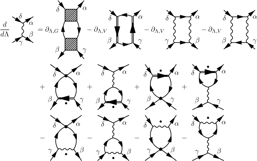
Figure 7: Diagrammatic representation of the two-loop renormalization group equation for the effective interaction in the (Nambu) particle-hole channel $V^{\text{PH},\Lambda}$. The first term on the right hand side represents the one-loop contributions where $\partial_{\Lambda,G}=\partial_{\Lambda,S}+\partial_{\Lambda,\Sigma}$ acts on fermionic propagators. The other terms in the first line represent two-loop box diagrams where $\partial_{\Lambda,V}$ is a shorthand for a scale-derivative acting on effective interactions and yielding the one-loop result. The other terms represent two-loop vertex correction diagrams where the effective interactions with dots represent the one-loop contribution.

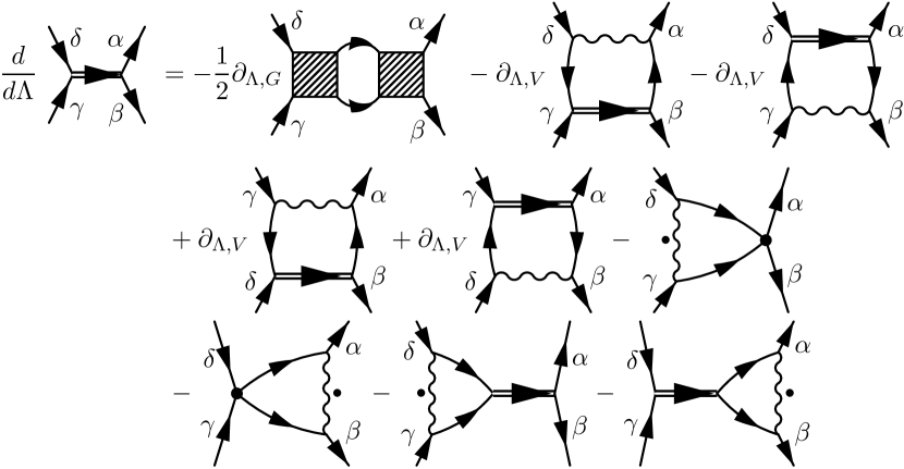
Figure 8: Diagrammatic representation of the two-loop renormalization group equation for the effective interaction in the (Nambu) particle-particle channel $V^{\text{PP},\Lambda}$. The first term on the right hand side represents the one-loop contribution. The last term in the second line and the contributions in the third line represent two-loop vertex correction diagrams. The other contributions are two-loop box diagrams. The notation is the same as in Fig. 7.

In the next section, we give a few remarks about the assignment of diagrams in the two-loop channel-decomposition scheme.

II.3 Discussion of assignment of diagrams

The channel-decomposition scheme derived in section II.2 is exact to the third order in the effective interaction. Due to the use of an approximation for the three-particle vertex of that order for its derivation, no $\dot{\Sigma}$-insertions appear in the scale-differentiated effective interactions in the two-loop contributions. However, within the same order of approximation the $\dot{\Sigma}$-insertions can be added to the scale-differentiated effective interactions in the two-loop contributions, because this introduces terms of $\mathcal{O}((\Gamma^{(4)\Lambda})^{4})$. The resulting channel-decomposition scheme would correspond to the two-loop flow equations for the two-particle vertex proposed by Veschgini and Salmhofer.Veschgini and Salmhofer (2013) For the attractive Hubbard model, we checked such an assignment and found only minor differences in the results in the presence of a not too small external pairing field. Note however that this may change in other contexts. For pairing field flows, including the $\dot{\Sigma}$-insertions in the two-loop contributions leads to a somewhat stronger renormalization of exchange propagators, but qualitatively similar results. In the numerical study of the attractive Hubbard model, we therefore did not include the $\dot{\Sigma}$-insertions in the two-loop contributions.

The scheme presented in the last section is relatively compact, because we only distinguished between singularities arising from fermionic propagators or effective interactions when assigning diagrams to interaction channels. For very small external pairing fields, it may be advantageous to further distinguish between one-loop box diagrams with normal or anomalous fermionic propagators. The reason is that the anomalous self-energy receives strong renormalizations in the pairing field flow due to the singular behavior of the amplitude mode. Insertions of the resulting $\dot{\Sigma}$ in the one-loop box diagrams may lead to artificial logarithmic singularities in non-Cooper channels when assigned as described above. These can be avoided by assigning the one-loop box diagrams with anomalous fermionic propagators in such a way that the transfer momentum is transported through the diagrams by the effective interactions. The one-loop box diagrams with normal fermionic propagators do not cause difficulties and should be assigned as described above. These subtleties matter only for very small external pairing fields (well beyond those that were accessible in the numerics). Therefore we decided to present the two-loop channel-decomposition scheme in the simpler form as above, but consider the more sophisticated version in the estimates in section III.2. We checked that the alternative assignment of one-loop box diagrams with anomalous propagators indeed yields very similar results in the numerically accessible range of external pairing fields.

III Attractive Hubbard model

In this section, we study the ground state of the attractive Hubbard model on the square lattice as a prototype for a singlet superfluid *[Forareview; see][]Micnas1990 using the two-loop channel-decomposition scheme. Progress in experiments with cold atoms in optical lattices sparked renewed research interest in this model in the last decade, because it can be simulated in such systems.Bloch et al. (2008); Esslinger (2010)

The attractive Hubbard model describes spin-$\frac{1}{2}$ fermions with a local attractive interaction on a lattice. Its Hamiltonian is

$$H=\sum_{i,j,\sigma}t_{ij}c^{\dagger}_{i\sigma}c_{j\sigma}+U\sum_{i}n_{i\uparrow}n_{i\downarrow},$$ (26)

where $c^{\dagger}_{i\sigma}$ and $c_{i\sigma}$ are creation and annihilation operators for fermions with spin orientation $\sigma$ on lattice site $i$. The interaction parameter $U$ is negative. The hopping of fermions is restricted to nearest- and next-nearest-neighbour sites with amplitudes $-t$ and $-t^{\prime}$, respectively, yielding the dispersion relation

$$\epsilon(\boldsymbol{k})=-2t(\cos k_{x}+\cos k_{y})-4t^{\prime}\cos k_{x}\cos k_{y}.\\$$ (27)

In the following, we use $t\equiv 1$ as the unit of energy.

The ground state of this model is an $s$-wave spin-singlet superfluid at any fermionic density. For $t^{\prime}=0$ and $n=1$ (half-filling), superfluidity is degenerate with charge-density wave order. The model has been studied in its ground state and at finite temperatures with a variety of methods, including resummations of perturbation theory,Fresard et al. (1992); Pedersen et al. (1997); Letz and Gooding (1998); Keller et al. (1999) quantum Randeria et al. (1992); Trivedi and Randeria (1995); Santos (1994); Singer et al. (1996) and variational Tamura and Yokoyama (2012) Monte Carlo methods, dynamical mean-field theory,Keller et al. (2001, 2002); Capone et al. (2002) and functional renormalization group.Gersch et al. (2008); Strack et al. (2008); Eberlein and Metzner (2013); Obert et al. (2013)

III.1 Parametrization and approximations

We now describe the approximate parametrization of the interaction vertex and self-energy, which allow for a numerical solution of the two-loop flow equations. The parametrizations are similar to those of Ref. Eberlein and Metzner, 2013.

In order to describe the superfluid state, we use Nambu fields (see Eq. (2)). In this representation, the fermionic propagator is a $2\times 2$ matrix and reads

$$\boldsymbol{G}^{\Lambda}(k)=\begin{pmatrix}G^{\Lambda}_{++}(k)&G^{\Lambda}_{+-}(k)\\ G^{\Lambda}_{-+}(k)&G^{\Lambda}_{--}(k)\end{pmatrix}=\begin{pmatrix}G^{\Lambda}(k)&F^{\Lambda}(k)\\ F^{\Lambda\ast}(k)&-G^{\Lambda}(-k),\end{pmatrix}$$ (28)

where $G^{\Lambda}(k)$ and $F^{\Lambda}(k)$ are its normal and anomalous components, respectively. The propagator is connected with the regularized bare propagator $\boldsymbol{G}_{0}^{\Lambda}$ and the Nambu self-energy $\boldsymbol{\Sigma}^{\Lambda}$ by the Dyson equation $(\boldsymbol{G}^{\Lambda})^{-1}=(\boldsymbol{G}_{0}^{\Lambda})^{-1}-\boldsymbol{\Sigma}^{\Lambda}$. $\boldsymbol{G}_{0}^{\Lambda}$ reads

$$\bigl{(}\boldsymbol{G}^{\Lambda}_{0}(k)\bigr{)}^{-1}=\begin{pmatrix}ik_{0}-\xi(\boldsymbol{k})-\delta\xi^{\Lambda}(\boldsymbol{k})+R^{\Lambda}(k_{0})&\Delta_{0}\\ \Delta_{0}&ik_{0}+\xi(\boldsymbol{k})+\delta\xi^{\Lambda}(\boldsymbol{k})+R^{\Lambda}(k_{0})\end{pmatrix},$$ (29)

where $\xi(\boldsymbol{k})=\epsilon(\boldsymbol{k})-\mu$ and $\delta\xi^{\Lambda}(\boldsymbol{k})$ is a counterterm. The regulator function

$$R^{\Lambda}(k_{0})=i\operatorname{sgn}(k_{0})\sqrt{k_{0}^{2}+\Lambda^{2}}-ik_{0}$$ (30)

regularizes the fermionic singularities by replacing small frequencies $k_{0}$ with $|k_{0}|\ll\Lambda$ by $\operatorname{sgn}(k_{0})\Lambda$. The external pairing field $\Delta_{0}$ appears in the bare propagator, because it serves as a regulator for pairing field flows,Eberlein and Metzner (2013) in which $\Delta_{0}$ is eliminated after integrating out the fermionic modes at $\Lambda>0$. The Nambu self-energy is given by

$$\boldsymbol{\Sigma}^{\Lambda}(k)=\begin{pmatrix}\Sigma^{\Lambda}(k)&\Delta_{0}-\Delta^{\Lambda}(k)\\ \Delta_{0}-\Delta^{\Lambda\ast}(k)&-\Sigma^{\Lambda}(-k)\end{pmatrix},$$ (31)

where the off-diagonal entries are chosen in such a way that the fermionic gap is $\Delta^{\Lambda}(k)$. The counterterm is related to the normal component of the self-energy via

$$\delta\xi^{\Lambda}(\boldsymbol{k})+\Sigma^{\Lambda}(0,\boldsymbol{k})=0$$ (32)

for $\boldsymbol{k}$ on the Fermi surface at all $\Lambda$, such that the Fermi surface remains fixed during the flow. Similar to Ref. Eberlein and Metzner, 2013, we neglect the momentum dependence of the self-energy but keep its dependence on frequency,

$$\Delta^{\Lambda}(k) =\Delta^{\Lambda}(k_{0}), \Sigma^{\Lambda}(k) =\Sigma^{\Lambda}(k_{0}), \delta\xi^{\Lambda}(\boldsymbol{k}) =\delta\xi^{\Lambda}.$$ (33)

The momentum dependence of the self-energy is not expected to be important at low fermionic densities, where the Fermi surface is almost circular. Furthermore, it lead only to minor changes of fRG flows for the weakly-coupled repulsive Hubbard model at van Hove filling.Giering and Salmhofer (2012) By choosing the external pairing field $\Delta_{0}$ to be real, we fix the phase of the anomalous self-energy so that $\Delta^{\Lambda}$ is also real. The frequency dependence of the self-energy is discretized on a grid of 30 points that is denser near $k_{0}=0$ and becomes sparser towards higher frequencies, with a maximal frequency around 300. Cubic spline interpolation is used to determine the self-energy at intermediate frequencies.

The interaction vertex is fully described by several coupling functions:Eberlein and Metzner (2010, 2013) $C^{\Lambda}_{kk^{\prime}}(q)$ and $M^{\Lambda}_{kk^{\prime}}(q)$ describe charge and spin fluctuations, respectively. The amplitude and phase mode of the superfluid gap are described by $A^{\Lambda}_{kk^{\prime}}(q)$ and $\Phi^{\Lambda}_{kk^{\prime}}(q)$. The imaginary part of the normal interaction in the Cooper channel is denoted as $P^{\prime\prime\Lambda}_{kk^{\prime}}(q)$. The real and imaginary part of the anomalous $(3+1)$ effective interaction is described by $X^{\prime\Lambda}_{kk^{\prime}}(q)$ and $X^{\prime\prime\Lambda}_{kk^{\prime}}(q)$, respectively. The coupling functions are expanded in exchange propagators that describe the singular dependence on the transfer momentum $q$ and fermion-boson vertices for the more regular dependences on the fermionic relative momenta $k$ and $k^{\prime}$. As in Ref. Eberlein and Metzner, 2013, we restrict this expansion to the $s$-wave channel and approximate the coupling functions by the following ansatz:

$$\begin{split}C^{\Lambda}_{kk^{\prime}}(q)&=C^{\Lambda}(q),\\ M^{\Lambda}_{kk^{\prime}}(q)&=M^{\Lambda}(q),\\ A^{\Lambda}_{kk^{\prime}}(q)&=A^{\Lambda}(q)g_{a}^{\Lambda}(k_{0})g_{a}^{\Lambda}(k_{0}^{\prime}),\\ \Phi^{\Lambda}_{kk^{\prime}}(q)&=\Phi^{\Lambda}(q)g_{\phi}^{\Lambda}(k_{0})g_{\phi}^{\Lambda}(k_{0}^{\prime}),\\ P^{\prime\prime\Lambda}_{kk^{\prime}}(q)&=P^{\prime\prime\Lambda}(q),\\ X^{\prime\Lambda}_{kk^{\prime}}(q)&=X^{\prime\Lambda}(q),\\ X^{\prime\prime\Lambda}_{kk^{\prime}}(q)&=X^{\prime\prime\Lambda}(q).\end{split}$$ (34)

In comparison to Ref. Eberlein and Metzner, 2013, we neglect the renormalization of the fermion-boson vertices in the particle-hole channel, for the anomalous $(3+1)$ effective interactions and for the imaginary part of the normal interaction in the Cooper channel. $g_{a}^{\Lambda}(k_{0})$ and $g_{\phi}^{\Lambda}(k_{0})$ are kept in order to obtain a meaningful frequency dependence of the gap function and to improve the fulfillment of the Ward identity for the global $U(1)$ charge symmetry. These simplifications are justified because the neglected frequency-dependences of fermion-boson vertices had only a minor influence on the flow at one-loop level. The effective interactions in the Nambu particle-hole and Nambu particle-particle channel then read

$$V^{\text{PH},\Lambda}_{s_{1}s_{2}s_{3}s_{4}}(q;k,k^{\prime}) =C^{\Lambda}(q)\tau^{(3)}_{s_{1}s_{4}}\tau^{(3)}_{s_{2}s_{3}}+M^{\Lambda}(q)\tau^{(0)}_{s_{1}s_{4}}\tau^{(0)}_{s_{2}s_{3}}$$

$$+\frac{1}{2}A^{\Lambda}(q)g_{a}^{\Lambda}(k_{0})g_{a}^{\Lambda}(k_{0}^{\prime})\tau^{(1)}_{s_{1}s_{4}}\tau^{(1)}_{s_{2}s_{3}}$$

$$+\frac{1}{2}\Phi^{\Lambda}(q)g_{\phi}^{\Lambda}(k_{0})g_{\phi}^{\Lambda}(k_{0}^{\prime})\tau^{(2)}_{s_{1}s_{4}}\tau^{(2)}_{s_{2}s_{3}}$$ (35)

$$+\frac{1}{2}P^{\prime\prime\Lambda}(q)(\tau^{(1)}_{s_{1}s_{4}}\tau^{(2)}_{s_{2}s_{3}}-\tau^{(2)}_{s_{1}s_{4}}\tau^{(1)}_{s_{2}s_{3}})$$

$$+X^{\prime}(q)(\tau^{(3)}_{s_{1}s_{4}}\tau^{(1)}_{s_{2}s_{3}}+\tau^{(1)}_{s_{1}s_{4}}\tau^{(3)}_{s_{2}s_{3}})$$

$$+X^{\prime\prime}(q)(\tau^{(3)}_{s_{1}s_{4}}\tau^{(2)}_{s_{2}s_{3}}-\tau^{(2)}_{s_{1}s_{4}}\tau^{(3)}_{s_{2}s_{3}}),$$

$$V^{\text{PP},\Lambda}_{s_{1}s_{2}s_{3}s_{4}}(q;k,k^{\prime}) =2M^{\Lambda}(q)\tau^{(2)}_{s_{1}s_{2}}\tau^{(2)}_{s_{3}s_{4}}$$ (36)

where $\tau^{(i)}$ are Pauli matrices ($i=1,2,3$) and the unit matrix ($i=0$). All functions in Eqs. (35) and (36) are even functions of momentum. $P^{\prime\prime\Lambda}$ and $X^{\prime\prime\Lambda}$ are odd functions of frequency, while all other functions are even. The frequency dependence of the fermion-boson vertices is discretized like for the self-energy. For the exchange propagators, we discretize the dependence on momenta and frequencies on a three-dimensional grid and trilinear interpolation is used at intermediate momenta and frequencies. The frequency dependence is discretized with 40 frequencies between $q_{0}=0$ and 300, with grid points denser at small frequencies. The momentum dependence is discretized with cylindrical coordinates around $\boldsymbol{q}=\boldsymbol{0}$ and $\boldsymbol{\pi}$, similar to Ref. Husemann and Salmhofer, 2009. The angular dependences are resolved with three angles between $0$ and $\pi/4$. At quarter-filling, the radial dependence of the singular exchange propagators $A(q)$, $\Phi(q)$, $P^{\prime\prime}(q)$ and $X^{\prime\prime}(q)$ around $\boldsymbol{q}=\boldsymbol{0}$ is discretized with 25 points between radius 0 and $\pi$, with denser distribution of points near $|\boldsymbol{q}|=0$. All other exchange propagators have a weaker dependence on momentum and are thus described with only 10 points in the radial direction.

The flow of the exchange propagators and fermion-boson vertices is extracted from the flow equations for the coupling functions as described in Ref. Eberlein and Metzner, 2013 by averaging the external fermionic momenta $\boldsymbol{k}$ and $\boldsymbol{k}^{\prime}$ over the Fermi surface for suitable choices of the transfer momentum and the fermionic frequencies. The flow of the exchange propagators is evaluated for $k_{0}=k_{0}^{\prime}=0$. The renormalization contributions to $g^{\Lambda}_{a}$ and $g^{\Lambda}_{\phi}$ are obtained after setting $q=0$ and $k_{0}^{\prime}=0$. The flow of the fermionic self-energy is evaluated similarly by averaging the external fermionic momentum over the Fermi surface.

By discretizing the dependences on momenta and frequencies, the functional flow equations were transformed into a system of around 20000 non-linear ordinary differential equations with three-dimensional loop integrals on the right-hand sides. These loop integrals were performed with an adaptive integration algorithm. The system of differential equations was integrated using an adaptive third-order Runge-Kutta routine. Depending on the parameters, the numerical integration of a flow on 32 CPU cores required around three days at one-loop level and between two and four weeks at two-loop level. Due to the large number of flowing couplings and the fact that the computations of their renormalization contributions are independent at a given scale, the flow equations are well suited for parallelization.

The numerical integration of the flow equations was started at a large finite scale $\Lambda_{0}\approx 100$, which is of the order of several times the band width. The fermionic modes for $\Lambda>\Lambda_{0}$ were treated in second-order perturbation theory, yielding exchange propagators of the order of $-U^{2}/\Lambda_{0}$ for $q=0$, so that the contributions from $\Lambda>\Lambda_{0}$ are small compared to $U$. Treating the high energy scales in perturbation theory also provides a well defined starting point for the flow of the fermion-boson vertices, which were set to one at $\Lambda_{0}$. The normal self-energy receives a sizeable contribution from the tadpole diagram at any finite $\Lambda_{0}$, yielding $\Sigma^{\Lambda_{0}}=-\delta\xi^{\Lambda_{0}}\approx U/2+\mathcal{O}(\Lambda_{0}^{-1})$. The anomalous self-energy $\Delta^{\Lambda_{0}}$ is determined self-consistently from the gap equation at scale $\Lambda_{0}$, but the corrections to $\Delta_{0}$ are small (of order $\mathcal{O}(U/\Lambda_{0})$).

Due to the truncation of the hierarchy of flow equations and the approximations for the coupling functions, the Ward identity for the global $U(1)$ charge symmetry is violated in the two-loop flows.Eberlein (2013) We did not systematically study how large these violation are quantitatively. For computing the results in section III.3, the Ward identity was enforced by a projection of the coupling constants as in Ref. Eberlein and Metzner, 2013. At low scales, this procedure effectively amounts to determining the Goldstone mass from the Ward identity instead of the flow equation.

III.2 Analytical estimates for infrared behavior

Before presenting results from numerical solutions of the flow equations, we discuss the infrared behavior of the vertex in a fermionic $s$-wave superfluid in the BCS regime at zero temperature. We assume that the fermionic modes at $\Lambda>0$ have been integrated out in the presence of an external pairing field $\Delta_{0}$. The latter regularizes the phase mode of the superfluid gap and is treated in a pairing field flow Eberlein and Metzner (2013) in this section. For simplicity, we assume a circular Fermi surface, but its shape is not expected to influence the conclusions. The infrared behavior at one-loop level was discussed in Ref. Eberlein and Metzner, 2013. In this section, we discuss only estimates for the most singular contributions to the flow at two-loop level. The flow equations including all terms are rather lengthy and can be found in Ref. Eberlein, 2013.

At small transfer momenta and frequencies, the exchange propagators in the Cooper channel and for the imaginary part of the anomalous (3+1) effective interaction are well described by

$$\begin{aligned} \Phi^{\Delta_{0}}(q)&\sim-\frac{1}{\Delta_{0}+Z_{\Phi}^{\Delta_{0}}q_{0}^{2}+A_{\Phi}^{\Delta_{0}}\boldsymbol{q}^{2}},\\ P^{\prime\prime\Delta_{0}}(q)&\sim-\frac{q_{0}}{\Delta_{0}+Z_{P^{\prime\prime}}^{\Delta_{0}}q_{0}^{2}+A_{P^{\prime\prime}}^{\Delta_{0}}\boldsymbol{q}^{2}},\\ X^{\prime\prime\Delta_{0}}(q)&\sim\frac{q_{0}}{\Delta_{0}+Z_{X^{\prime\prime}}^{\Delta_{0}}q_{0}^{2}+A_{X^{\prime\prime}}^{\Delta_{0}}\boldsymbol{q}^{2}},\\ A^{\Delta_{0}}(q)&\sim-\frac{1}{\sqrt{\Delta_{0}+Z_{A}^{\Delta_{0}}q_{0}^{2}+A_{A}^{\Delta_{0}}\boldsymbol{q}^{2}}},\end{aligned}$$ (37)

where the superscripts indicate that $\Delta_{0}$ is the flow parameter. The ansätze for $\Phi^{\Delta_{0}}$, $P^{\prime\prime\Delta_{0}}$ and $X^{\prime\prime\Delta_{0}}$ are consistent with a resummation of all chains of Nambu particle-hole diagrams Eberlein and Metzner (2013) and can be justified non-perturbatively for $\Phi^{\Delta_{0}}$ and $P^{\prime\prime\Delta_{0}}$ using Ward identities.Castellani et al. (1997); Pistolesi et al. (2004) The ansatz for $A^{\Delta_{0}}$ is consistent with the expected singular infrared behavior of the amplitude mode in an interacting Bose gas and reproduces the singular infrared scaling that was described in Refs. Strack et al., 2008; Obert et al., 2013 in terms of divergent wave function renormalization factors. The above-mentioned works indicate that the coefficients $A_{i}^{\Delta_{0}}$ and $Z_{i}^{\Delta_{0}}$ in the ansätze remain finite when defined as above. We assume that all other exchange propagators are less singular in the limit where the external pairing field vanishes. Below we show that these assumptions are justified and the ansätze consistent with the infrared behavior of the flow. The fermion-boson vertices are set to one in this section, as they are not expected to influence the singular behavior.

In the presence of a superfluid gap and close to the Fermi surface, the fermionic propagator behaves like

$$\begin{aligned} F^{\Delta_{0}}(k+p)&\approx\frac{1}{\Delta^{\Delta_{0}}},\\ G^{\Delta_{0}}(k+p)&\approx-\frac{ip_{0}+v_{F}\boldsymbol{p}\cdot\boldsymbol{e}_{\boldsymbol{k}_{F}}}{(\Delta^{\Delta_{0}})^{2}}\end{aligned}$$ (38)

for small $p$ and $k=(0,\boldsymbol{k}_{F})$, together with appropriate ultraviolet cutoffs, where $v_{F}$ is the Fermi velocity and $\boldsymbol{e}_{\boldsymbol{k}_{F}}$ a unit vector pointing in the direction of $\boldsymbol{k}_{F}$. In this section, we neglect the normal self-energy and assume that it can be subsumed into Fermi liquid like renormalization factors, which do not influence the singular infrared behavior as they remain finite (see below).

The most singular contributions at two-loop level arise from diagrams involving scale-derivatives of the phase mode. The two-loop vertex correction diagrams of this kind involve an integral of the form

$$\int\negthickspace\negthinspace\frac{d^{3}p}{(2\pi)^{3}}\partial_{\Delta_{0}}\Phi^{\Delta_{0}}(p),$$ (39)

where we suppressed the fermionic propagators and the second effective interaction. The integrals should be evaluated with some ultraviolet cutoff arising from the decay of the fermionic propagators at high frequencies and the lattice. In case the integrals do not cause problems at the upper integration limit, we send the cutoffs to infinity as the interesting behavior arises from the region around $p=0$. Neglecting the contributions from the (finite) $\Delta_{0}$-derivatives of the renormalization factors for the dependence on momenta and frequencies, this integral yields

$$\int\negthickspace\negthinspace\frac{d^{3}p}{(2\pi)^{3}}\frac{1}{(\Delta_{0}+Z^{\Delta_{0}}_{\Phi}p_{0}^{2}+A^{\Delta_{0}}p^{2})^{2}}\sim\frac{1}{A^{\Delta_{0}}_{\Phi}\sqrt{Z^{\Delta_{0}}_{\Phi}\Delta_{0}}}.$$ (40)

In the following, the renormalization factors for the momentum and frequency dependences are suppressed, as they are assumed to be finite and non-singular in the limit of a vanishing external pairing field and thus do not change the infrared behavior qualitatively. When multiplying this contribution with a finite effective interaction, as in the flow equations for the exchange propagators in the particle-hole channel, it may give rise to non-analytic behavior but not to divergences as a function of $\Delta_{0}$ after integrating the flow. In the flow equations for the exchange propagators in the particle-particle channel, more singular contributions appear either from propagator renormalization or two-loop box diagrams.

The two-loop box diagrams are potentially more singular than the vertex correction diagrams, as they contain loops with two exchange propagators for the phase mode. The biggest change in the infrared behavior in comparison to the one-loop approximation is found for the amplitude mode $A^{\Delta_{0}}$. Evaluating the two-loop box diagram for external momenta $k=k^{\prime}=(0,\boldsymbol{k}_{F})$, the leading contributions read

$$\begin{split}\frac{d}{d\Delta_{0}}&A^{\Delta_{0}}(0)|_{\text{2L}}\sim-\int\negthickspace\negthinspace\frac{d^{3}p}{(2\pi)^{3}}\Bigl{[}F(k+p)^{2}\\ &\times\partial_{\Delta_{0}}\bigl{(}A^{\Delta_{0}}(p)^{2}+\Phi^{\Delta_{0}}(p)^{2}-8X^{\prime\prime\Delta_{0}}(p)^{2}+P^{\prime\prime\Delta_{0}}(p)^{2}\bigr{)}\\ &+8\operatorname{Im}G(k+p)F(k+p)\partial_{\Delta_{0}}\bigl{(}X^{\prime\prime\Delta_{0}}(p)\Phi^{\Delta_{0}}(p)\bigr{)}\Bigr{]}\\ &+\ldots.\end{split}$$ (41)

The ellipsis represents less singular terms in $\Delta_{0}$ that either involve less singular exchange propagators or where their singularities are suppressed by momentum and frequency factors stemming from the fermionic propagators. The most singular contribution arises from the squared exchange propagator for the phase mode, for which an estimate yields

$$\begin{split}\frac{d}{d\Delta_{0}}A^{\Delta_{0}}(0)|_{\text{2L}}&\sim\int\negthickspace\negthinspace\frac{d^{3}p}{(2\pi)^{3}}\Phi^{\Delta_{0}}(p)\frac{d}{d\Delta_{0}}\Phi^{\Delta_{0}}(p)\\ &\sim\Delta_{0}^{-3/2}.\end{split}$$ (42)

After integration, this gives rise to the expected infrared scaling behavior of the amplitud mode,Castellani et al. (1997); Pistolesi et al. (2004); Strack et al. (2008); Obert et al. (2013) expressed in terms of an external pairing field,

$$A^{\Delta_{0}}(0)\sim\Delta_{0}^{-1/2}.$$ (43)

More generally, in dimension $2<d<4$ it reads $A^{\Delta_{0}}(0)\sim\Delta_{0}^{(d-4)/2}$, which is similar to the behavior of the longitudinal susceptibility in the non-linear sigma model in an external magnetic field Belitz et al. (2005) (here, the case $d=2+1$ is relevant).

The leading contributions to the charge mode look similar to Eq. (41), but with the anomalous fermionic propagators replaced by normal ones,

$$\begin{split}\frac{d}{d\Delta_{0}}&C^{\Delta_{0}}(0)|_{\text{2L}}\sim-\int\negthickspace\negthinspace\frac{d^{3}p}{(2\pi)^{3}}\operatorname{Re}G(k+p)^{2}\\ &\times\partial_{\Delta_{0}}\bigl{(}A^{\Delta_{0}}(p)^{2}+\Phi^{\Delta_{0}}(p)^{2}\bigr{)}+\ldots\end{split}$$ (44)

The momentum factors resulting from the normal propagators weaken the singularity of $\Phi^{\Delta_{0}}(p)^{2}$, so that the integral yields $\tfrac{d}{d\Delta_{0}}C^{\Delta_{0}}(0)|_{\text{2L}}\sim\Delta_{0}^{-1/2}$ and thus $C^{\Delta_{0}}(0)|_{\text{2L}}\sim\Delta_{0}^{1/2}+\operatorname{const}$. The leading renormalization contribution to the anomalous (3+1) effective interaction reads

$$\begin{split}\frac{d}{d\Delta_{0}}&X^{\prime\Delta_{0}}(0)|_{\text{2L}}\sim-\int\negthickspace\negthinspace\frac{d^{3}p}{(2\pi)^{3}}\operatorname{Re}G(k+p)F(k+p)\\ &\times\partial_{\Delta_{0}}\bigl{(}\Phi^{\Delta_{0}}(p)^{2}-A^{\Delta_{0}}(p)^{2}\bigr{)}+\ldots\end{split}$$ (45)

and is slightly more singular than $\tfrac{d}{d\Delta_{0}}C^{\Delta_{0}}(0)|_{\text{2L}}$ due to the presence of one anomalous fermionic propagator. A simple estimate hints at a logarithmic singularity of $X^{\prime\Delta_{0}}(0)$, but its prefactor vanishes due to the approximate particle-hole symmetry in the vicinity of the Fermi surface. In the magnetic channel, the two-loop box diagrams yield a logarithmically singular contribution to $\frac{d}{d\Delta_{0}}M^{\Delta_{0}}(0)|_{\text{2L}}$, which does not give rise to singular behavior after integration. The two-loop contributions to the phase mode are less singular than the propagator renormalization diagrams. Note that simple estimates as above for propagator renormalization diagrams with $\dot{\Sigma}$-insertions would yield a contribution to the phase mode that diverges as $\Delta_{0}^{-3/2}$. Such a divergence would be inconsistent with Eq. (37) and would lead to a drastic violation of the $U(1)$ Ward identity. We did not detect such a contribution numerically (see section III.3), potentially due to cancellations caused by Ward identities.

The change in the infrared behavior of the vertex also impacts the self-energy. The normal self-energy does not receive singular contributions, as $C^{\Delta_{0}}(0)$ and $X^{\prime\Delta_{0}}(0)$ remain finite and the fluctuation contributions are integrable in two dimensions at zero temperature. The flow of the anomalous self-energy is altered due to the singular behavior of $A^{\Delta_{0}}(0)\sim\Delta_{0}^{-1/2}$ to

$$\begin{split}\frac{d}{d\Delta_{0}}\Delta^{\Delta_{0}}&=-A^{\Delta_{0}}(0)\int\negthickspace\negthinspace\frac{d^{3}p}{(2\pi)^{3}}S_{F}^{\Delta_{0}}(p)+\ldots\\ &\sim\Delta_{0}^{-1/2},\end{split}$$ (46)

where $S_{F}^{\Delta_{0}}$ is the anomalous component of the single-scale propagator, which depends only weakly on $\Delta_{0}$. At one-loop level, one obtains $\tfrac{d}{d\Delta_{0}}\Delta^{\Delta_{0}}\sim\mathcal{O}(1)$. The anomalous self-energy thus becomes non-analytic at two-loop level as a function of the external pairing field,

$$\Delta^{\Delta_{0}}-\Delta^{\Delta_{0}=0}\sim\Delta_{0}^{1/2}.$$ (47)

More generally, this result reads $\Delta^{\Delta_{0}}-\Delta^{\Delta_{0}=0}\sim\Delta_{0}^{(d-2)/2}$ in $2<d<4$ dimensions. Such a non-analytic behavior is also found in the magnetization of the non-linear sigma model in an external magnetic field.Belitz et al. (2005)

III.3 Numerical results

We now present results for the effective interactions and the self-energy from numerical solutions of the flow equations at two-loop level for a quarter-filled system ($n=1/2$), where the Fermi surface is almost circular. The results were obtained by first integrating out the fermionic modes at $\Lambda>0$ in the presence of an external pairing field of the order of $\Delta_{\text{MF}}/100$, where $\Delta_{\text{MF}}$ is the mean-field gap, and subsequently reducing the external pairing field in another flow.

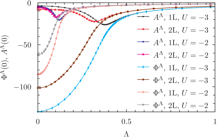
Figure 9: (Color online) Renormalization group flow of the amplitude ($A^{\Lambda}$) and phase ($\Phi^{\Lambda}$) coupling functions at fixed external pairing field at one-loop (1L) and two-loop (2L) level for different interactions $U$ for $n=1/2$, $t^{\prime}=-0.1$ and $\Delta_{0}\approx\Delta_{\text{MF}}/100$.

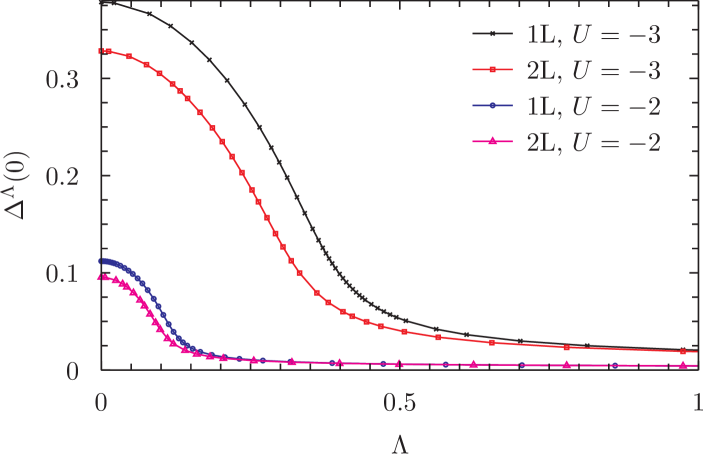
Figure 10: (Color online) Renormalization group flow of the superfluid gap at fixed external pairing field at one-loop (1L) and two-loop (2L) level for different interactions $U$ for $n=1/2$, $t^{\prime}=-0.1$ and $\Delta_{0}\approx\Delta_{\text{MF}}/100$.

In the presence of a not too small external pairing field, the flows at two-loop level are qualitatively similar to those at one-loop level. This can be seen in Fig. 9, which shows the flow of the amplitude and phase mode of the gap at vanishing momentum and frequency, $A^{\Lambda}(0)$ and $\Phi^{\Lambda}(0)$, for a quarter-filled ($n=1/2$) system with $t^{\prime}=-0.1$ for different values of $U$. The critical scales $\Lambda_{c}$ (the scales where $|A^{\Lambda}(0)|$ is maximal) are, however, reduced due to fluctuation corrections at two-loop level. The same observations can be made for the flow of the anomalous self-energy at zero frequency, which is shown in Fig. 10 for the same parameters as in Fig. 9. In the presence of a not too small external pairing field and for $|U|\leq 3$, the $\Lambda$-dependence of the anomalous self-energy is still qualitatively similar to that in mean-field theory, $\Delta^{\Lambda}\approx\sqrt{\Lambda_{c}^{2}-\Lambda^{2}}$ for $\Lambda<\Lambda_{c}$, even at two-loop level. This means that the critical scale and gap are mainly reduced by fluctuations above $\Lambda_{c}$. For smaller external pairing fields or larger values of $|U|$, the agreement worsens because the gap at $\Lambda=0$ gets somewhat larger than expected from the above relation. This indicates an increasing impact of phase fluctuations and is accompanied by a change in the behavior of $A^{\Lambda}(0)$ for small $\Lambda$. Instead of a monotonic decrease in absolute value below the critical scale as shown in Fig. 9, $A^{\Lambda}(0)$ first decreases in absolute value below the critical scale and then slightly increases at low scales. For $\Delta_{0}\approx\Delta_{\text{MF}}/100$, this effect was either absent ($|U|\leq 3$) or small, so that long-range phase fluctuations were mostly treated in the pairing field flows.

The momentum and frequency dependence of the self-energy and exchange propagators is qualitatively similar to the one-loop approximation.Eberlein and Metzner (2013) The same holds for the flows of the effective interactions in the magnetic, charge and anomalous (3+1) channels. We therefore do not show results for these quantities.

The impact of phase fluctuations can be studied in a controlled way by eliminating the external pairing field in a second flow. The results of such pairing field flows are shown in Figs. 11, 12 and 13. Figure 11 shows the reduction of the anomalous self-energy in pairing field flows at one- and two-loop level for $U=-3$, $t^{\prime}=-0.1$ and $n=1/2$, which is mainly caused by amplitude and long-range phase fluctuations. Depending on the initial size of the external pairing field, the anomalous self-energy is reduced around 10 % in the pairing field flow, with a slightly stronger reduction for larger initial external pairing fields. The $\Delta_{0}$-dependence of the gap at one- and two-loop level is linear to a very good approximation. This is expected at one-loop level. At two-loop level, the numerically accessible external pairing fields are too large for resolving the expected non-analytic behavior on the scale of Fig. 11. Fitting $\Delta^{\Delta_{0}}=a+b\Delta_{0}^{1/2}+c\Delta_{0}$ to the $\Delta_{0}$-dependence of the gap at two-loop level yields only a small coefficient for the term $\sim\Delta_{0}^{1/2}$.

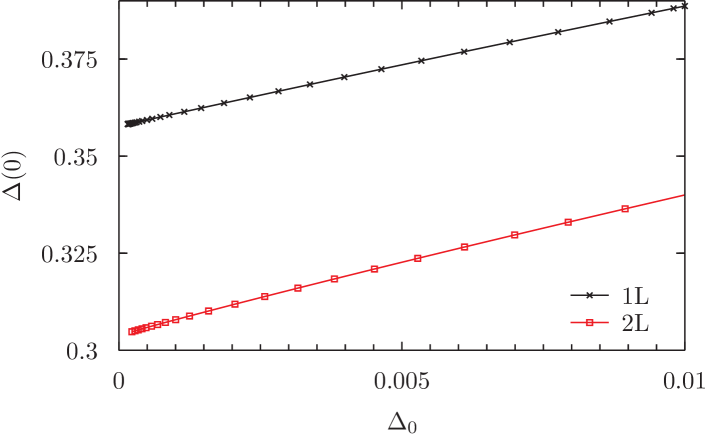
Figure 11: (Color online) Pairing field flow of the anomalous self-energy at one-loop (1L) and two-loop (2L) level for $U=-3$, $t^{\prime}=-0.1$ and $n=1/2$. The external pairing field $\Delta_{0}$ is used as the flow parameter and was chosen as $\Delta_{0}=\Delta_{\text{MF}}/50$ in the fermionic flow.

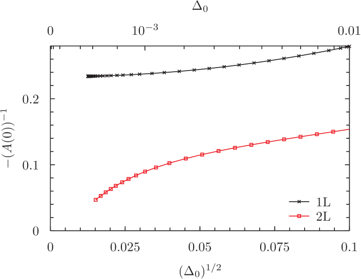
Figure 12: (Color online) Pairing field flow of the amplitude coupling function $A$ at one-loop (1L) and two-loop (2L) level for the same parameters as in Fig. 11.

Figure 13: (Color online) Pairing field flow of the inverse of the derivatives of the amplitude $A$ and phase $\Phi$ coupling functions with respect to the external pairing field $\Delta_{0}$ at two-loop level for the same parameters as in Fig. 11. The red and magenta lines are fits to the expected dependence on the external pairing field (see text). For a better presentation, the result for the phase mode is rescaled by factors of $50$.

The amplitude mode $A^{\Delta_{0}}$ gets strongly renormalized during the pairing field flow as can be seen in Fig. 12, which compares the one- and two-loop approximations for a quarter-filled system with $U=-3$ and $t^{\prime}=-0.1$. In both cases, the flows for $\Lambda>0$ were computed in the presence of an external pairing field $\Delta_{0}=\Delta_{\text{MF}}/50$, which was reduced by a factor $\approx 50$ in the pairing field flow. Smaller external pairing fields were not accessible within our framework of approximations due to remnants of the violation of the Ward identity for the global $U(1)$ charge symmetry that cannot be cured with the abovementioned simple projection method for enforcing the Ward identity. The results in Fig. 12 are plotted in such a way that the scaling in Eq. (43) would yield a linear dependence near $\Delta_{0}=0$. Fluctuations at two-loop level clearly lead to a strong renormalization of the amplitude mode and tend to suppress $(-A(0))^{-1}$ towards zero. However, due to the limited range of accessible pairing fields, the behavior in the limit $\Delta_{0}\rightarrow 0$ is not apparent from this plot. From the numerical data, we also cannot draw conclusions on the behavior of the effective interactions in the particle-hole channel in this limit for the same reason. Figure 13 shows the inverse of the derivatives of the amplitude and phase coupling functions at $q=0$ with respect to the external pairing field as computed during the same pairing field flow as in Fig. 12. From Eq. (37) and (42) one expects $(\text{d}\Phi/\text{d}\Delta_{0})(0)\propto\Delta_{0}^{-2}$ and $(\text{d}A/\text{d}\Delta_{0})(0)\propto\Delta_{0}^{-3/2}$. In Fig. 13, the numerical results are compared to fits using the function $f(\Delta_{0})=a+b\Delta_{0}^{n}$, where $n=2$ for $(\text{d}\Phi/\text{d}\Delta_{0})^{-1}$ and $n=3/2$ for $(\text{d}A/\text{d}\Delta_{0})^{-1}$, showing good agreement with the expected dependence on $\Delta_{0}$. The small offsets near $\Delta_{0}=0$ are remnants of the violation of the Ward identity for the global $U(1)$ charge symmetry.

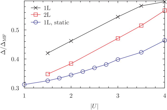
Figure 14: (Color online) Gap ratio $\Delta/\Delta_{\text{MF}}$ as a function of $U$ from one-loop (1L) and two-loop (2L) flows for $n=1/2$ and $t^{\prime}=-0.1$. Also shown are results from a static approximation (1L, static) in which all frequency dependences are neglected.

Figures 9 and 10 already gave an impression of the renormalization of the critical scale and the gap by fluctuations at two-loop level. The impact of these fluctuations also depends on the size of $U$. This can be seen in Fig. 14, which shows the gap ratio $\Delta/\Delta_{\text{MF}}$ as a function of the interaction for a quarter-filled system with $t^{\prime}=-0.1$. $\Delta=\Delta(0)$ is the gap as obtained from extrapolating pairing field flows to the limit $\Delta_{0}\rightarrow 0$ and $\Delta_{\text{MF}}$ is the gap in mean-field approximation. The one-loop results are in very good agreement with those of Ref. Eberlein and Metzner, 2013 despite the differences in the approximations for the momentum and frequency dependence of exchange propagators. The observed increase of $\Delta/\Delta_{\text{MF}}$ with $|U|$ is consistent with the behavior in the limits $U\rightarrow 0^{-}$ and $U\rightarrow-\infty$. These limits are accessible in perturbation theory Georges and Yedidia (1991); Martín-Rodero and Flores (1992) or by mapping the attractive Hubbard model at finite doping to the Heisenberg model in a magnetic field, respectively. Results for the staggered magnetization in the latter were obtained numerically in Ref. Lüscher and Läuchli, 2009. In the coupling range considered, the gaps at two-loop level are 5 - 20 % smaller than at one-loop level. For smaller values of $|U|$, it is difficult to compute the gap from a numerical solution of the flow equations, because the gap and the critical scale decrease exponentially. It is expected that the two-loop result approaches the one-loop result for smaller values of $U$, because the phase space for fluctuations at two-loop level decreases with $|U|$. It is interesting that the gap ratios at one- and two-loop level approach each other with increasing $|U|$. This may indicate that the Katanin scheme overestimates certain fluctuation contributions, which are compensated by two-loop contributions with overlapping loops at larger $|U|$. Figure 14 also shows results from a static one-loop approximation, in which the frequency dependence of the self-energy and vertex is neglected. Note that the gaps from this approximation are even smaller than those from the two-loop approximation, indicating that the former overestimates the impact of fluctuations when using the frequency regulator in Eq. (30).

IV Summary

We have analyzed flow equations for the two-particle vertex in the fermionic functional renormalization group at two-loop level and reformulated them effectively as one-loop equations. In two-loop contributions with overlapping loops, the insertion of two vertices that are connected by a full and a single-scale propagator can be reexpressed through the one-loop result for the scale-derivative of the vertex. This is similar in spirit to the replacement of tadpole insertions by scale-derivatives of the self-energy in the Katanin scheme. The reformulation is exact to the third order in the effective interaction, sheds light on the physics described by the two-loop renormalization contributions, and allows for their efficient numerical treatment.

The proposed scheme is based on a decomposition of the vertex in charge, magnetic and pairing channels. Using this decomposition, the singular dependence of the vertex on momenta and frequencies can be described within a reasonable numerical effort also at two-loop level. The scheme allows to continue renormalization group flows into phases with broken symmetries, which we demonstrated for the superfluid ground state of the attractive Hubbard model.

Using simple estimates for the most singular diagrams, we analyzed the infrared behavior of the vertex and the self-energy in the ground state of an $s$-wave superfluid in the BCS regime. We find that the two-loop scheme captures the expected singular behavior of the amplitude mode as well as the non-analytic behavior of the order parameter in the limit where the external pairing field vanishes. In a description using auxiliary bosons for the order parameter, this infrared behavior is governed by a non-Gaussian fixed point.Pistolesi et al. (2004); Strack et al. (2008) Thus, our approach captures non-Gaussian fluctuations, although the related fixed point structure is less transparent than in the partially bosonized approach.

We argue that the vertex in the ground state of a fermionic $s$-wave superfluid in two dimensions does not exhibit infrared singularities beyond those in the Cooper channel that are already known from the singular infrared behavior of interacting bosons. Our formalism yields a unified description of the reduction of the anomalous self-energy by particle-hole and collective fluctuations. In comparison to the one-loop approximation, the obtained superfluid order parameters at two-loop order are slightly smaller.

The formalism presented in this article may be useful also in other contexts. As it treats all interaction channels on equal footing and captures single-particle as well as collective fluctuations, it might be a convenient tool for the study of competing orders in systems of correlated fermions, like the repulsive Hubbard model, possibly in conjunction with mean-field theory for the low-energy modes below the scale for symmetry breaking.Wang et al. (2014) Quite generally, it may be helpful for applying the fermionic functional renormalization group at larger interactions.