Hessian Recovery for Finite Element Methods

Abstract.

In this article, we propose and analyze an effective Hessian recovery strategy for the Lagrangian finite element method of arbitrary order. We prove that the proposed Hessian recovery method preserves polynomials of degree $k+1$ on general unstructured meshes and superconverges at a rate of $O(h^{k})$ on mildly structured meshes. In addition, the method is proved to be ultraconvergent (two order higher) for translation invariant finite element space of any order. Numerical examples are presented to support our theoretical results.

1. Introduction

Post-processing is an important technique in scientific computing, where it is necessary to draw some useful information that have physical meanings such as velocity, flux, stress, etc., from the primary results of the computation. These quantities of interest usually involve derivatives of the primary data. Some popular post-processing techniques include the celebrated Zienkiewicz-Zhu superconvergent patch recovery (SPR) [26], polynomial preserving recovery (PPR) [25, 15], and edge based recovery [19], which were proposed to obtain accurate gradients with reasonable cost. Similarly, post-processing for second order derivatives, which are related to physical quantities such as momentum and Hessian, are also desirable. Hessian matrix is particularly significant in adaptive mesh design, since it can indicate the direction where the function changes the most and guide us to construct anisotropic meshes to cope with the anisotropic properties of the solution of the underlying partial differential equation [2, 4]. It also plays an important role in finite element approximation of second order non-variational elliptic problems [12], numerical solution of some fully nonlinear equations such as Monge-Amp$\grave{\text{e}}$re equation [13, 16], and designing nonlocal finite element technique [7].

There have been some works in literature on this subject. In 1998, Lakhany-Whiteman used a simple averaging twice at edge centers of the regular uniform triangular mesh to produce a superconvergent Hessian [11]. Later, some other reseachers such as Agouzal et al. [1] and Ovall [18] also studied Hessian recovery. Comparsion studies of existing Hessian recovery techniques are found in Vallet et al. [21] and Picasso et al. [20]. However, there is no systematic theory guarantees convergence in general circumstances. Moreover, there are certain technical difficulties in obtaining rigorous convergence proof for meshes other than the regular pattern triangular mesh. In a very recent work, Kamenski-Huang argued that it is not necessary to have very accurate or even convergent Hessian in order to obtain a good mesh [10].

Our current work is not targeted on the direction of adaptive mesh refinement; instead, our emphasis is to obtain accurate Hessian matrices via recovery techniques. We propose an effective Hessian recovery method and establish a solid theoretical analysis for such a recovery method. Our approach is to apply PPR twice to the primarily computed data. This idea is natural. However, the mathematical theory behind is non-trivial and quite involved, especially in the ultraconvergence analysis of the recovered Hessian. A direct calculation of the gradient from the linear finite element space has linear convergent rate and the Hessian has no convergence at all. Our Hessian recovery can achieve second-order convergence under some uniform meshes, which is a very surprising result!

2. Preliminaries

In this section, we first introduce some frequently used notation and then briefly describe the polynomial preserving recovery (PPR) operator [25, 15], which is the basis of our Hessian recovery method.

2.1. Notation

Let $\Omega$ be a bounded polygonal domain with Lipschitz boundary $\partial\Omega$ in $\mathbb{R}^{2}$. Throughout this article, the standard notation for classical Sobolev spaces and their associate norms are adopted as in [3, 5]. A multi-index $\alpha$ is a $2$-tuple of non-negative integers $\alpha_{i}$, $i=1,2$. The length of $\alpha$ is given by

$$|\alpha|=\sum_{i=1}^{2}\alpha_{i}.$$

For $u\in W^{k}_{p}(\Omega)$ and $|\alpha|\leq k$, denote $D^{\alpha}u$ the weak partial derivative $(\frac{\partial}{\partial x})^{\alpha_{1}}(\frac{\partial}{\partial y})^{\alpha_{2}}u$. Also, $D^{k}u$ with $|\alpha|=k$ is the vector of all partial derivatives of order $k$. The Hessian operator $H$ is denoted by

(2.1) $$H=\begin{pmatrix}\partial_{xx}&\partial_{xy}\\ \partial_{yx}&\partial_{yy}\end{pmatrix}.$$

For a subdomain $\mathcal{A}$ of $\Omega$, let $\mathbb{P}_{m}(\mathcal{A})$ be the space of polynomials of degree less than or equal to $m$ over $\mathcal{A}$ and $n_{m}$ be the dimension of $\mathbb{P}_{m}(\mathcal{A})$ with $n_{m}=\frac{1}{2}(m+1)(m+2)$. $W^{k}_{p}(\mathcal{A})$ denotes the classical Sobolev space with norm $\|\cdot\|_{k,p,\mathcal{A}}$ and seminorm $|\cdot|_{k,p,\mathcal{A}}$. When $p=2$, we denote simply $H^{k}(\mathcal{A})=W^{k}_{2}(\mathcal{A})$ and the subscript $p$ is omitted.

For any $0<h<\frac{1}{2}$, let $\mathcal{T}_{h}$ be a shape regular triangulation of $\bar{\Omega}$ with mesh size at most $h$, i.e.

$$\bar{\Omega}=\bigcup_{K\in\mathcal{T}_{h}}K,$$

where $K$ is a triangle. For any $k\in\mathbb{N}$, define the continuous finite element space $S_{h}$ of order $k$ as

$$S_{h}=\{v\in C(\bar{\Omega}):v|_{K}\in\mathbb{P}_{k}(K),\quad\forall K\in\mathcal{T}_{h}\}\subset H^{1}(\Omega).$$

Let $\mathcal{N}_{h}$ denote the set of mesh nodes, i.e. the dual space of $S_{h}$. The standard Lagrange basis of $S_{h}$ is denoted by $\{\phi_{z}:z\in\mathcal{N}_{h}\}$ with $\phi_{z}(z^{\prime})=\delta_{zz^{\prime}}$ for all $z,z^{\prime}\in\mathcal{N}_{h}$. For any $v\in H^{1}(\Omega)\cap C(\Omega)$, let $v_{I}$ be the interpolation of $v$ in $S_{h}$, i.e.,$v_{I}=\sum\limits_{z\in\mathcal{N}_{h}}v(z)\phi_{z}$.

For $\mathcal{A}\subset\Omega$, let $S_{h}(\mathcal{A})$ denote the restrictions of functions in $S_{h}$ to $\mathcal{A}$ and let $S_{h}^{\text{comp}}(\mathcal{A})$ denote the set of those functions in $S_{h}(\mathcal{A})$ with compact support in the interior of $\mathcal{A}$ [22]. Let $\Omega_{0}\subset\subset\Omega_{1}\subset\subset\Omega_{2}\subset\subset\Omega$ be separated by $d\geq c_{o}h$ and $\ell$ be a direction, i.e., a unit vector in $\mathbb{R}^{2}$. Let $\tau$ be a parameter, which will typically be a multiply of $h$. Let $T^{\ell}_{\tau}$ denote translation by $\tau$ in the direction $\ell$, i.e.,

(2.2) $$T^{\ell}_{\tau}v(x)=v(x+\tau\ell),$$

and for an integer $\nu$

(2.3) $$T^{\ell}_{\nu\tau}v(x)=v(x+\nu\tau\ell).$$

Following the definition of [22], the finite element space $S_{h}$ is called translation invariant by $\tau$ in the direction $\ell$ if

(2.4) $$T^{\ell}_{\nu\tau}v\in S^{\text{comp}}_{h}(\Omega),\quad\forall v\in S^{\text{comp}}_{h}(\Omega_{1}),$$

for some integer $\nu$ with $|\nu|<M$. Equivalently, $\mathcal{T}_{h}$ is called a translation invariant mesh. To clarify the matter, we consider five popular triangular mesh patterns: Regular, Chevron, Union-Jack, Criss-cross, and equilateral patterns, as shown in Figure 1.

Figure 1. Five types of uniform meshes: (a) Regular pattern; (b) Chevron pattern; (c) Criss-cross pattern; (d) Union-Jack pattern; (e) Equilateral pattern

We see that:

1) Regular pattern is translation invariant by $h$ in directions $(1,0)$ and $(0,1)$, by $2\sqrt{2}h$ in directions $(\pm\frac{\sqrt{2}}{2},\frac{\sqrt{2}}{2})$, and by $\sqrt{5}h$ in directions $(\frac{2\sqrt{5}}{5},\pm\frac{\sqrt{5}}{5})$ and $(\pm\frac{\sqrt{5}}{5},\frac{2\sqrt{5}}{5})$, ……

2) Chevron pattern is translation invariant by $h$ in the direction $(0,1)$, by $2h$ in the direction $(1,0)$, and by $2\sqrt{2}h$ in directions $(\pm\frac{\sqrt{2}}{2},\frac{\sqrt{2}}{2})$, and by $\sqrt{5}h$ in directions $(\pm\frac{\sqrt{5}}{5},\frac{2\sqrt{5}}{5})$, ……

3) Criss-cross pattern is translation invariant by $\sqrt{2}h$ in directions $(1,0)$ and $(0,1)$, and by $2h$ in directions $(\pm\frac{\sqrt{2}}{2},\frac{\sqrt{2}}{2})$, ……

4) Union-Jack pattern is translation invariant by $2h$ in directions $(1,0)$ and $(0,1)$, and by $2\sqrt{2}h$ in directions $(\pm\frac{\sqrt{2}}{2},\frac{\sqrt{2}}{2})$, ……

5) Equilateral pattern is translation invariant by $h$ in directions $(1,0)$ and $(\pm\frac{1}{2},\frac{\sqrt{3}}{2})$, and by $\sqrt{3}h$ in directions $(0,1)$ and $(\frac{\sqrt{3}}{2},\pm\frac{1}{2})$, ……

Throughout this article, the letter $C$ or $c$, with or without subscript, denotes a generic constant which is independent of $h$ and may not be the same at each occurrence. To simplify notation, we denote $x\leq Cy$ by $x\lesssim y$.

2.2. Polynomial preserving recovery

Let $G_{h}:S_{h}\rightarrow S_{h}\times S_{h}$ be the PPR operator. Given a function $u_{h}\in S_{h}$, it suffices to define $(G_{h}u_{h})(z)$ for all $z\in\mathcal{N}_{h}$. Let $z\in\mathcal{N}_{h}$ be a vertex and $\mathcal{K}_{z}$ be a patch of elements around $z$ which is defined in [25, 15]. Select all nodes in $\mathcal{N}_{h}\cap\mathcal{K}_{z}$ as sampling points and fit a polynomial $p_{z}\in\mathbb{P}_{k+1}(\mathcal{K}_{z})$ in the least squares sense at those sampling points, i.e.

(2.5) $$p_{z}=\arg\min_{p\in\mathbb{P}_{k+1}(\mathcal{K}_{z})}\sum_{\tilde{z}\in\mathcal{N}_{h}\cap\mathcal{K}_{z}}(u_{h}-p)^{2}(\tilde{z}).$$

Then the recovered gradient at $z$ is defined as

$$(G_{h}u_{h})(z)=\nabla p_{z}(z).$$

For linear element, all nodes in $\mathcal{N}_{h}$ are vertices and hence $G_{h}u_{h}$ is well defined. However, $\mathcal{N}_{h}$ may contain edge nodes or interior nodes for higher order elements. If $z$ is an edge node which lies on an edge between two vertices $z_{1}$ and $z_{2}$, we define

$$(G_{h}u_{h})(z)=\beta\nabla p_{z_{1}}(z)+(1-\beta)\nabla p_{z_{2}}(z)$$

where $\beta$ is determined by the ratio of distances of $z$ to $z_{1}$ and $z_{2}$. If $z$ is an interior node which lies in a triangle formed by three vertices $z_{1}$, $z_{2}$, and $z_{3}$, we define

$$(G_{h}u_{h})(z)=\sum_{j=1}^{3}\beta_{j}\nabla p_{z_{j}}(z),$$

where $\beta_{j}$ is the barycentric coordinate of $z$.

Remark 2.1.

It was proved in [14] that certain rank condition and geometric condition guarantee the uniqueness of $p_{z}$ in (2.5).

Remark 2.2.

In order to avoid numerical instability, a discrete least squares fitting process is carried out on a reference patch $\omega_{z}$ .

3. Hessian recovery method

Given $u\in S_{h}$, let $G_{h}u\in S_{h}\times S_{h}$ be the recovered gradient using PPR as defined in previous section. We rewrite $G_{h}u$ as

(3.1) $$G_{h}u=\begin{pmatrix}G_{h}^{x}u\\ G_{h}^{y}u\end{pmatrix}.$$

In order to recover the Hessian matrix of $u$, we apply gradient recovery operator $G_{h}$ to $G_{h}^{x}u$ and $G_{h}^{y}u$ one more time, respectively, and define the Hessian recovery operator $H_{h}$ as follows

(3.2) $$H_{h}u=\begin{pmatrix}G_{h}(G_{h}^{x}u),&G_{h}(G_{h}^{y}u)\end{pmatrix}=\begin{pmatrix}G_{h}^{x}(G_{h}^{x}u)&G_{h}^{x}(G_{h}^{y}u)\\ G_{h}^{y}(G_{h}^{x}u)&G_{h}^{y}(G_{h}^{y}u)\end{pmatrix}.$$

Just as PPR, we obtain $H_{h}:S_{h}\rightarrow S_{h}^{2}\times S_{h}^{2}$ on the whole domain $\Omega$ by interpolation after determining values of $H_{h}u$ at all nodes in $\mathcal{N}_{h}$.

Remark 3.1.

The two gradient recovery operators in definition (3.2) of $H_{h}$ can be different. Actually we can define the Hessian recovery operator $H_{h}$ as following

$$H_{h}u=\begin{pmatrix}\tilde{G}_{h}(G_{h}^{x}u),&\tilde{G}_{h}(G_{h}^{y}u)\end{pmatrix}.$$

By choosing $G_{h}$ and $\tilde{G}_{h}$ as PPR or SPR operator, we obtain four different Hessian recovery operators, i.e., PPR-PPR, PPR-SPR, SPR-PPR, and SPR-SPR. However, numerical tests have shown that PPR-PPR is the best one.

In order to demonstrate our method, we shall discuss two examples in detail. For the sake of simplicity, only linear element on uniform meshes will be considered. In practice, the method can be applied to arbitrary meshes and higher order elements.

Example 1. Consider the regular pattern uniform mesh as in Figure 3. We want to recovery the Hessian matrix at $z_{0}$. As deduced in [25], the recovered gradient at $z_{0}$ is given by

$$(G_{h}u)(z_{0})=\frac{1}{6h}\left(\begin{pmatrix}2\\ 1\end{pmatrix}u_{1}+\begin{pmatrix}1\\ 2\end{pmatrix}u_{2}+\begin{pmatrix}-1\\ 1\end{pmatrix}u_{3}+\begin{pmatrix}-2\\ -1\end{pmatrix}u_{4}+\begin{pmatrix}-1\\ -2\end{pmatrix}u_{5}+\begin{pmatrix}1\\ -1\end{pmatrix}u_{6}\right).$$

Here $u_{i}=u(z_{i}),(i=0,1,\ldots 18)$ represents function value of $u$ at node $z_{i}$. Thus, according to the definition (3.2) of the Hessian recovery operator $H_{h}$, we have

(3.3) $$\begin{split}\begin{pmatrix}H^{xx}_{h}u\\ H^{xy}_{h}u\end{pmatrix}(z_{0})=\frac{1}{6h}\left(2(G_{h}u)(z_{1})+(G_{h}u)(z_{2})-(G_{h}u)(z_{3})-\right.\\ \left.2(G_{h}u)(z_{4})-(G_{h}u)(z_{5})+(G_{h}u)(z_{6})\right),\end{split}$$

and

(3.4) $$\begin{split}\begin{pmatrix}H^{yx}_{h}u\\ H^{yy}_{h}u\end{pmatrix}(z_{0})=\frac{1}{6h}\left((G_{h}u)(z_{1})+2(G_{h}u)(z_{2})+(G_{h}u)(z_{3})-\right.\\ \left.(G_{h}u)(z_{4})-2(G_{h}u)(z_{5})-(G_{h}u)(z_{6})\right),\end{split}$$

where

$$(G_{h}u)(z_{1})=\frac{1}{6h}\left(\begin{pmatrix}2\\ 1\end{pmatrix}u_{7}+\begin{pmatrix}1\\ 2\end{pmatrix}u_{8}+\begin{pmatrix}-1\\ 1\end{pmatrix}u_{2}+\begin{pmatrix}-2\\ -1\end{pmatrix}u_{0}+\begin{pmatrix}-1\\ -2\end{pmatrix}u_{18}+\begin{pmatrix}1\\ -1\end{pmatrix}u_{6}\right),$$

and $(G_{h}u)(z_{2}),\ldots,(G_{h}u)(z_{6})$ follow the similar pattern. Direct calculation reveals that

$$(H_{h}^{xx}u)(z_{0})=\frac{1}{36h^{2}}( -12u_{0}+2u_{1}-4u_{2}-4u_{3}+2u_{4}-4u_{5}-4u_{6}+4u_{7}+4u_{8}+u_{9}$$

$$-2u_{10}+u_{11}+4u_{12}+4u_{13}+4u_{14}+u_{15}-2u_{16}+u_{17}+4u_{18}),$$

$$(H_{h}^{xy}u)(z_{0})=\frac{1}{36h^{2}}( 6u_{0}-u_{1}+5u_{2}-u_{3}-u_{4}+5u_{5}-u_{6}-2u_{7}+u_{8}+u_{9}$$

$$+u_{10}-2u_{11}-5u_{12}-2u_{13}+u_{14}+u_{15}+u_{16}-2u_{17}-5u_{18}),$$

$$(H_{h}^{yx}u)(z_{0})=\frac{1}{36h^{2}}( 6u_{0}-u_{1}+5u_{2}-u_{3}-u_{4}+5u_{5}-u_{6}-2u_{7}+u_{8}+u_{9}$$

$$+u_{10}-2u_{11}-5u_{12}-2u_{13}+u_{14}+u_{15}+u_{16}-2u_{17}-5u_{18}),$$

$$(H_{h}^{yy}u)(z_{0})=\frac{1}{36h^{2}}( -12u_{0}-4u_{1}-4u_{2}+2u_{3}-4u_{4}-4u_{5}+2u_{6}+u_{7}-2u_{8}+u_{9}$$

$$+4u_{10}+4u_{11}+4u_{12}+u_{13}-2u_{14}+u_{15}+4u_{16}+4u_{17}+4u_{18}).$$

It is observed that $(H^{xy}_{h}u)(z_{0})=(H^{yx}_{h}u)(z_{0})$, which means the recovered Hessian matrix is symmetric, a property of the exact Hessian we would like to maintain.

Using Taylor expansion, we can show that

$$(H_{h}^{xx}u)(z_{0})=u_{xx}(z_{0})+\frac{h^{2}}{3}(u_{xxxx}(z_{0})+u_{xxxy}(z_{0})+u_{xxyy}(z_{0}))+O(h^{4}),$$

$$(H_{h}^{xy}u)(z_{0})=u_{xy}(z_{0})+\frac{h^{2}}{3}(u_{xxxy}(z_{0})+u_{xxyy}(z_{0})+u_{xyyy}(z_{0}))+O(h^{4}),$$

$$(H_{h}^{yx}u)(z_{0})=u_{yx}(z_{0})+\frac{h^{2}}{3}(u_{xxxy}(z_{0})+u_{xxyy}(z_{0})+u_{xyyy}(z_{0}))+O(h^{4}),$$

$$(H_{h}^{yy}u)(z_{0})=u_{yy}(z_{0})+\frac{h^{2}}{3}(u_{xxyy}(z_{0})+u_{xyyy}(z_{0})+u_{yyyy}(z_{0}))+O(h^{4}),$$

which imply that $H_{h}u$ provides a second order approximation of $Hu$ at $z_{0}$.

Example 2. Consider the Chevron pattern uniform mesh as shown in Figure 3. Repeating the procedure as in Example 1, we derive the recovered Hessian matrix at $z_{0}$ as

$$(H_{h}^{xx}u)(z_{0})=\frac{1}{144h^{2}}( -72u_{0}+36u_{13}+36u_{7}),$$

$$(H_{h}^{xy}u)(z_{0})=\frac{1}{144h^{2}}( -12u_{1}+12u_{3}+24u_{4}-24u_{6}+6u_{7}+$$

$$+36u_{9}-36u_{11}-6u_{13}+6u_{14}-6u_{18}),$$

$$(H_{h}^{yx}u)(z_{0})=\frac{1}{144h^{2}}( 12u_{1}-12u_{3}+36u_{4}-36u_{6}-6u_{7}+$$

$$6u_{8}+24u_{9}-24u_{11}-6u_{12}+6u_{13}),$$

$$(H_{h}^{yy}u)(z_{0})=\frac{1}{144h^{2}}( -48u_{0}-10u_{1}-22u_{2}-10u_{3}-10u_{4}+18u_{5}-$$

$$10u_{6}-2u_{7}+u_{8}+10u_{9}+36u_{10}+10u_{11}+u_{12}-$$

$$2u_{13}+u_{14}+10u_{15}+16u_{16}+10u_{17}+u_{18}).$$

In addition, we have the following Taylor expansion

$$(H_{h}^{xx}u)(z_{0})=u_{xx}(z_{0})+\frac{h^{2}}{3}u_{xxxx}(z_{0})+\frac{2h^{4}}{45}u_{xxxxxx}(z_{0})+O(h^{5}),$$

$$(H_{h}^{xy}u)(z_{0})=u_{xy}(z_{0})+\frac{h^{2}}{12}(3u_{xxxy}(z_{0})+2u_{xyyy}(z_{0}))-\frac{h^{3}}{24}u_{xxxyy}(z_{0})+O(h^{4}),$$

$$(H_{h}^{yx}u)(z_{0})=u_{yx}(z_{0})+\frac{h^{2}}{12}(3u_{xxxy}(z_{0})+2u_{xyyy}(z_{0}))+\frac{h^{3}}{24}u_{xxxyy}(z_{0})+O(h^{4}),$$

$$(H_{h}^{yy}u)(z_{0})=u_{yy}(z_{0})+\frac{h^{2}}{6}(u_{xxyy}(z_{0})+2u_{yyyy}(z_{0}))-\frac{5h^{3}}{72}u_{xxyyy}(z_{0})+O(h^{4}).$$

We conclude that $H_{h}u$ is a second order approximation to the Hessian matrix. It is worth pointing out that, though $H_{h}^{xy}\neq H_{h}^{yx}$ for the Chevron pattern uniform mesh, they are both second order finite difference schemes at $z_{0}$.

Remark 3.2.

PPR-PPR is the only one among the four Hessian recovery methods mentioned in Remark 3.1 that provides second order approximation for all five mesh patterns, especially the Chevron pattern.

Figure 2. Regular Pattern

Figure 3. Chevron Pattern

Both example 1 and 2 indicate that for linear element the PPR-PPR approach is equivalent to a finite difference scheme of second order accuracy at vertex $z_{0}$. In general, we can show that $H_{h}$ preserves polynomials of degree up to $k+1$ for $k$th order element.

Consider $P_{k}$-element. Let $u$ be a polynomial of degree $k+1$. Since $G_{h}$ preserves polynomials of degree $k+1$, it follows that $G_{h}u=\nabla u$ which is a polynomial of degree $k$. Therefore, we have

(3.5) $$H_{h}u=(G_{h}(G^{x}_{h}u),G_{h}(G^{y}_{h}u))=(G_{h}\frac{\partial u}{\partial x},G_{h}\frac{\partial u}{\partial x})=(\nabla\frac{\partial u}{\partial x},\nabla\frac{\partial u}{\partial x})=Hu.$$

It means that $H_{h}$ preserves polynomials of degree $k+1$ for arbitrary mesh.

Now we proceed translation invariant mesh. Under the polynomial preserving property, the recovered gradient is exact for polynomials of degree $k+1$. Therefore

(3.6) $$G_{h}^{x}u=D_{x}u+h^{k+1}\boldsymbol{a}^{x}\cdot D^{k+2}u+h^{k+2}\boldsymbol{b}^{x}\cdot D^{k+3}u+h^{k+3}\boldsymbol{c}^{x}\cdot D^{k+4}u+\cdots;$$

(3.7) $$G_{h}^{y}u=D_{y}u+h^{k+1}\boldsymbol{a}^{y}\cdot D^{k+2}u+h^{k+2}\boldsymbol{b}^{y}\cdot D^{k+3}u+h^{k+3}\boldsymbol{c}^{y}\cdot D^{k+4}u+\cdots.$$

Note that $\boldsymbol{a}^{x},\boldsymbol{a}^{y},\boldsymbol{b}^{x},\boldsymbol{b}^{y},\boldsymbol{c}^{x},\boldsymbol{c}^{y},\cdots$ are functions of $(x,y)$ if $z=(x,y)$ a nodal point of arbitrary mesh.

Let $\boldsymbol{z}=(x,y)$ be any node on a translation invariant mesh. We further assume that $\boldsymbol{z}$ is a local symmetry center for all sampling points involved. Notice that coefficients $\boldsymbol{a}^{x}$, $\boldsymbol{a}^{y}$, $\boldsymbol{b}^{x}$, $\boldsymbol{b}^{y},\ldots$ depend only on the coordinates of nodes, since we recover gradient at nodes only. Thus for translation invariant meshes, $\boldsymbol{a}^{x}$, $\boldsymbol{a}^{y}$, $\boldsymbol{b}^{x}$, $\boldsymbol{b}^{y},\ldots$ are constants. In addition, due to symmetry, it makes no difference if we perform $G^{x}_{h}$ or $G^{y}_{h}$ first. Hence,

(3.8) $$\begin{split}&(H_{h}^{xy}u)(\boldsymbol{z})=(G_{h}^{y}(G_{h}^{x}u))(\boldsymbol{z})\\ =&G_{h}^{y}[D_{x}u(\boldsymbol{z})+h^{k+1}\boldsymbol{a}^{x}\cdot D^{k+2}u(\boldsymbol{z})+h^{k+2}\boldsymbol{b}^{x}\cdot D^{k+3}u(\boldsymbol{z})+\cdots]\\ =&(G_{h}^{y}(D_{x}u))(\boldsymbol{z})+h^{k+1}(\boldsymbol{a}^{x}\cdot G_{h}^{y}(D^{k+2}u))(\boldsymbol{z})+h^{k+2}(\boldsymbol{b}^{x}\cdot G_{h}^{y}(D^{k+3}u))(\boldsymbol{z})+\cdots\\ =&(D_{y}D_{x}u)(\boldsymbol{z})+h^{k+1}(\boldsymbol{a}^{y}\cdot D^{k+2}D_{x}u)(\boldsymbol{z})+h^{k+2}(\boldsymbol{b}^{y}\cdot D^{k+3}D_{x}u)(\boldsymbol{z})\\ &+h^{k+1}(\boldsymbol{a}^{x}\cdot D_{y}(D^{k+2}u))(\boldsymbol{z})+h^{k+2}(\boldsymbol{b}^{x}\cdot D_{y}(D^{k+3}u))(\boldsymbol{z})+O(h^{k+3})\\ =&(D_{y}D_{x}u)(\boldsymbol{z})+h^{k+1}[\boldsymbol{a}^{y}\cdot D^{k+2}D_{x}u+\boldsymbol{a}^{x}\cdot D_{y}(D^{k+2}u)](\boldsymbol{z})+\\ &h^{k+2}[\boldsymbol{b}^{y}\cdot D^{k+3}D_{x}u+\boldsymbol{b}^{x}\cdot D_{y}(D^{k+3}u)](\boldsymbol{z})+O(h^{k+3}).\end{split}$$

Notice that (3.8) is valid only at nodal points. Similarly,

(3.9) $$\begin{split}(H_{h}^{yx}u)(\boldsymbol{z})=&(D_{x}D_{y}u)(\boldsymbol{z})+h^{k+1}[\boldsymbol{a}^{x}\cdot D^{k+2}D_{y}u+\boldsymbol{a}^{y}\cdot D_{x}(D^{k+2}u)](\boldsymbol{z})+\\ &h^{k+2}[\boldsymbol{b}^{x}\cdot D^{k+3}D_{y}u+\boldsymbol{b}^{y}\cdot D_{x}(D^{k+3}u)](\boldsymbol{z})+O(h^{k+3});\end{split}$$

(3.10) $$\begin{split}(H_{h}^{xx}u)(\boldsymbol{z})=&(D_{x}D_{x}u)(\boldsymbol{z})+h^{k+1}[\boldsymbol{a}^{x}\cdot D^{k+2}D_{x}u+\boldsymbol{a}^{x}\cdot D_{x}(D^{k+2}u)](\boldsymbol{z})+\\ &h^{k+2}[\boldsymbol{b}^{x}\cdot D^{k+3}D_{x}u+\boldsymbol{b}^{x}\cdot D_{x}(D^{k+3}u)](\boldsymbol{z})+O(h^{k+3});\end{split}$$

(3.11) $$\begin{split}(H_{h}^{yy}u)(\boldsymbol{z})=&(D_{y}D_{y}u)(z)+h^{k+1}[\boldsymbol{a}^{y}\cdot D^{k+2}D_{y}u+\boldsymbol{a}^{y}\cdot D_{y}(D^{k+2}u)](\boldsymbol{z})+\\ &h^{k+2}[\boldsymbol{b}^{y}\cdot D^{k+3}D_{y}u+\boldsymbol{b}^{y}\cdot D_{y}(D^{k+3}u)](\boldsymbol{z})+O(h^{k+3}).\end{split}$$

(3.8)–(3.11) imply that the Hessian recovery operator $H_{h}$ is exact for polynomials of degree $k+2$ for translation invariant meshes. Also, we observe $H_{h}^{xy}=H_{h}^{yx}$ from (3.8) and (3.9).

It is worth pointing out that, except for the Chevron pattern, (3.8)–(3.11) are valid for the other four patterns of uniform meshes, since the recovered gradient $G_{h}u$ produces the same stencil at each node.

Next we consider even order ($k=2r)$ element on translation invariant meshes, in which case

(3.12) $$\boldsymbol{a}^{x}(\boldsymbol{z})=\boldsymbol{0},\quad\boldsymbol{c}^{x}(\boldsymbol{z})=\boldsymbol{0},\quad\boldsymbol{a}^{y}(\boldsymbol{z})=\boldsymbol{0},\quad\boldsymbol{c}^{y}(\boldsymbol{z})=\boldsymbol{0};$$

(3.13) $$D\boldsymbol{a}^{x}(\boldsymbol{z})=\boldsymbol{0},\quad D\boldsymbol{c}^{x}(\boldsymbol{z})=\boldsymbol{0},\quad D\boldsymbol{a}^{y}(\boldsymbol{z})=\boldsymbol{0},\quad D\boldsymbol{c}^{y}(\boldsymbol{z})=\boldsymbol{0}.$$

and $\boldsymbol{b}^{x},\boldsymbol{b}^{y},\cdots$ are constants in (3.7). Here the symbol $D$ is understood as taking all partial derivatives to each entry of the vector. Consequently,

(3.14) $$(G_{h}^{y}u)(\boldsymbol{z})=(D_{y}u)(\boldsymbol{z})+h^{k+2}(\boldsymbol{b}^{y}\cdot D^{k+3}u)(\boldsymbol{z})+O(h^{k+4}),$$

Also, (3.14) is valid only at nodal points. Plugging (3.6) into (3.14) yields

$$\begin{split}&(H_{h}^{xy}u)(\boldsymbol{z})=(G_{h}^{y}G_{h}^{x}u)(\boldsymbol{z})\\ =&(D_{y}G_{h}^{x}u)(\boldsymbol{z})+h^{k+2}(\boldsymbol{b}^{y}\cdot D^{k+3}G_{h}^{x}u)(\boldsymbol{z})+O(h^{k+4})\\ =&D_{y}(D_{x}u+h^{k+1}\boldsymbol{a}^{x}\cdot D^{k+2}u+h^{k+2}\boldsymbol{b}^{x}\cdot D^{k+3}u+h^{k+3}\boldsymbol{c}^{x}\cdot D^{k+4}u\\ &+\cdots)(\boldsymbol{z})+h^{k+2}(\boldsymbol{b}^{y}\cdot D^{k+3}D_{x}u)(\boldsymbol{z})+O(h^{k+4})\\ =&(D_{y}D_{x}u)(\boldsymbol{z})+h^{k+2}(\boldsymbol{b}^{x}\cdot D_{y}D^{k+3}u+\boldsymbol{b}^{y}\cdot D^{k+3}D_{x}u)(\boldsymbol{z})+O(h^{k+4}).\end{split}$$

In the last identity we have used (3.12) and (3.13).

The argument for the other three entries of recovered Hessian matrix are similar. We conclude that the Hessian recovery operator $H_{h}$ is exact for polynomials of degree up to $k+3$ when $k$ is even and the mesh is translation invariant and symmetric with respect to $x$ and $y$.

The above results can be summarized as the following theorem:

Theorem 3.3.

The Hessian recovery operator $H_{h}$ preserves polynomials of degree $k+1$ for an arbitrary mesh. If $z$ is a node of a translation invariant mesh, then $H_{h}$ preserves polynomials of degree $k+2$ for odd $k$, and of degree $k+3$ for even $k$. Moreover, if the sampling points are symmetric with respect to $x$ and $y$, then $H_{h}$ is symmetric.

Remark 3.4.

According to [21], the best Hessian recovery method in the literature preserves polynomial of degree 2 for linear element. Our method preserves polynomial of degree 2 on general unstructured meshes and preserves polynomials of degree 3 on translation invariant meshes for linear element.

Theorem 3.5.

Let $u\in W_{\infty}^{k+2}(\mathcal{K}_{z})$; then

$$\|Hu-H_{h}u\|_{0,\infty,\mathcal{K}_{z}}\lesssim h^{k}|u|_{k+2,\infty,\mathcal{K}_{z}}.$$

If $z$ is a node of translation invariant mesh and $u\in W_{\infty}^{k+3}(\mathcal{K}_{z})$, then

$$|(Hu-H_{h}u)(z)|\lesssim h^{k+1}|u|_{k+3,\infty,\mathcal{K}_{z}}.$$

Furthermore, if $z$ is a node of translation invariant mesh and $u\in W_{\infty}^{k+4}(\mathcal{K}_{z})$ with $k$ an even number, then

$$|(Hu-H_{h}u)(z)|\lesssim h^{k+2}|u|_{k+4,\infty,\mathcal{K}_{z}}.$$

Proof.

It is a direct result of Theorem 3.3 and application of the Hilbert-Bramble Lemma. ∎

4. Superconvergence analysis

In this section, we first use the supercloseness between the gradient of the finite element solution $u_{h}$ and the gradient of the interpolation $u_{I}$ [2, 4, 8, 9, 23, 24], and properties of the PPR operator [25, 14] to establish the superconvergence property of our Hessian recovery operator on mildly structured mesh. Then we utilize the tool of superconvergence by difference quotients from [22] to prove the proposed Hessian recovery method is ultraconvergent for translation invariant finite element space of any order.

In this section, we consider the following variational problem: find $u\in H^{1}(\Omega)$ such that

(4.1) $$B(u,v)=\int_{\Omega}(\mathcal{D}\nabla u+\mathbf{b}u)\cdot\nabla v+cuvdx=(f,v),\quad\forall v\in H^{1}(\Omega).$$

Here $\mathcal{D}$ is a $2\times 2$ symmetric positive definite matrix, $\mathbf{b}$ is a vector, and $c$ as well as $f$ are scalars. All coefficient functions are assumed to be smooth.

In order to insure (4.1) has a unique solution, we assume the bilinear form $B(\cdot,\cdot)$ satisfies the continuity condition

(4.2) $$|B(u,v)|\leq\nu\|u\|_{1,\Omega}\|v\|_{1,\Omega},$$

for all $u,v\in H^{1}(\Omega)$. We also assume the inf-sup conditions [5, 3, 2]

(4.3) $$\inf_{u\in H^{1}(\Omega)}\sup_{v\in H^{1}(\Omega)}\frac{B(u,v)}{\|u\|_{1,\Omega}\|v\|_{1,\Omega}}=\sup_{u\in H^{1}(\Omega)}\inf_{v\in H^{1}(\Omega)}\frac{B(u,v)}{\|u\|_{1,\Omega}\|v\|_{1,\Omega}}\geq\mu>0.$$

The finite element approximation of (4.1) is to find $u_{h}\in S_{h}$ satisfying

(4.4) $$B(u_{h},v_{h})=(f,v_{h}),\quad\forall v_{h}\in S_{h}.$$

To insure a unique solution for (4.4), we assume the inf-sup conditions

(4.5) $$\inf_{u\in S_{h}}\sup_{v\in S_{h}}\frac{B(u,v)}{\|u\|_{1,\Omega}\|v\|_{1,\Omega}}=\sup_{u\in S_{h}}\inf_{v\in S_{h}}\frac{B(u,v)}{\|u\|_{1,\Omega}\|v\|_{1,\Omega}}\geq\mu>0.$$

From (4.1) and (4.4), it is easy to see that

(4.6) $$B(u-u_{h},v)=0$$

for any $v\in S_{h}$. In particular, (4.6) holds for any $v\in S^{\text{comp}}_{h}(\Omega)$.

4.1. Linear element

Linear finite element space $S_{h}$ on quasi-uniform mesh $\mathcal{T}_{h}$ is considered in this subsection.

Definition 4.1.

The triangulation $\mathcal{T}_{h}$ is said to satisfy Condition $(\sigma,\alpha)$ if there exist a partition $\mathcal{T}_{h,1}\cup\mathcal{T}_{h,2}$ of $\mathcal{T}_{h}$ and positive constants $\alpha$ and $\sigma$ such that every two adjacent triangles in $\mathcal{T}_{h,1}$ form an $O(h^{1+\alpha})$ parallelogram and

$$\sum_{T\in{\mathcal{T}_{h,2}}}|T|=O(h^{\sigma}).$$

An $O(h^{1+\alpha})$ parallelogram is a quadrilateral shifted from a parallelogram by $O(h^{1+\alpha})$.

For general $\alpha$ and $\sigma$, Xu and Zhang [24] proved the following theorem.

Theorem 4.2.

Let $u$ be the solution of (4.1), let $u_{h}\in S_{h}$ be the finite element solution of (4.4), and let $u_{I}\in S_{h}$ be the linear interpolation of $u$. If the triangulation $\mathcal{T}_{h}$ satisfies Condition $(\sigma,\alpha)$ and $u\in H^{3}(\Omega)\cap W^{2}_{\infty}(\Omega)$, then

$$|u_{h}-u_{I}|_{1,\Omega}\lesssim h^{1+\rho}(|u|_{3,\Omega}+|u|_{2,\infty,\Omega}),$$

where $\rho=\min(\alpha,\sigma/2,1/2)$.

Using the above result, we are able to obtain a convergence rate for our Hessian recovery operator.

Theorem 4.3.

Suppose that the solution of (4.1) belongs to $H^{3}(\Omega)\cap W^{2}_{\infty}(\Omega)$ and $\mathcal{T}_{h}$ satisfies Condition $(\sigma,\alpha)$, then we have

$$\|Hu-H_{h}u_{h}\|_{0,\Omega}\leq h^{\rho}\|u\|_{3,\infty,\Omega}.$$

Proof.

We decompose $Hu-H_{h}u_{h}$ as $(Hu-H_{h}u)+H_{h}(u_{I}-u_{h})$, since $H_{h}u=H_{h}u_{I}$. Using the triangle inequality and the definition of $H_{h}$, we obtain

$$\|Hu-H_{h}u_{h}\|_{0,\Omega} \leq\|Hu-H_{h}u\|_{0,\Omega}+\|H_{h}(u_{I}-u_{h})\|_{0,\Omega}$$

$$=\|Hu-H_{h}u\|_{0,\Omega}+\|G_{h}(G_{h}(u_{I}-u_{h}))\|_{0,\Omega}.$$

The first term in the above expression is bounded by $h|u|_{3,\infty,\Omega}$ according to Theorem 3.5. Since $G_{h}$ is a bounded linear operator [15], it follows that

$$\|H_{h}(u_{I}-u_{h})\|_{0,\Omega}\lesssim\|\nabla(G_{h}(u_{I}-u_{h}))\|_{0,\Omega}$$

Notice that $G_{h}(u_{I}-u_{h})$ is a function in $S_{h}$ and hence the inverse estimate [5, 3] can be applied. Thus,

$$\|H_{h}(u_{I}-u_{h})\|_{0,\Omega}\lesssim h^{-1}\|G_{h}(u_{I}-u_{h})\|_{0,\Omega}\lesssim h^{-1}\|u_{I}-u_{h}\|_{1,\Omega}$$

and hence Theorem 4.2 implies that

$$\|H_{h}(u_{I}-u_{h})\|_{0,\Omega}\lesssim h^{\rho}\|u\|_{3,\infty,\Omega}.$$

Combining the above two estimates completes our proof. ∎

4.2. Quadratic element

We proceed to quadratic finite element space $S_{h}$. According to [9], a triangulation $\mathcal{T}_{h}$ is strongly regular if any two adjacent triangles in $\mathcal{T}_{h}$ form an $O(h^{2})$ approximate parallelogram. Huang and Xu proved the following superconvergence results in [9].

Theorem 4.4.

If the triangulation $\mathcal{T}_{h}$ is uniform or strongly regular, then

$$|u_{h}-u_{I}|_{1,\Omega}\lesssim h^{3}|u|_{4,\Omega}.$$

Based on the above theorem, we obtain the following superconvergent result.

Theorem 4.5.

Suppose that the solution of (4.1) belongs to $H^{4}(\Omega)$ and $\mathcal{T}_{h}$ is uniform or strongly regular. Then we have

$$\|Hu-H_{h}u_{h}\|_{0,\Omega}\leq h^{2}\|u\|_{4,\Omega}.$$

Proof.

The proof is similar to the proof of Theorem 4.3 by using Theorem 4.4 and the inverse estimate. ∎

Remark 4.6.

Theorem 4.5 can be generalized to mildly structured meshes as in [9].

4.3. Translation invariant element of any order

First, we observe that the Hessian recovery operator results in a difference quotient. It is due to the fact that $G_{h}$ is a difference quotient [25] and the composition of two difference quotients is still a difference quotient. Let us take linear element on uniform triangular mesh of the regular pattern as an example, see Figure 3. The recovered second order derivative at a nodal point $z$ is

$$\begin{split}(H_{h}^{xx}u_{h})(z)=\frac{1}{36h^{2}}(&-12u_{0}+2u_{1}-4u_{2}-4u_{3}+2u_{4}-4u_{5}-4u_{6}+4u_{7}+4u_{8}+u_{9}\\ &-2u_{10}+u_{11}+4u_{12}+4u_{13}+4u_{14}+u_{15}-2u_{16}+u_{17}+4u_{18}).\end{split}$$

Let $\phi_{j}$ be the nodal shape functions. Since $\phi_{z}(z^{\prime})=\delta_{zz^{\prime}}$, it follows that

$$(H_{h}^{xx}u_{h})\phi_{0}(x,y)$$

$$= \frac{1}{36h^{2}}[-12u_{0}\phi_{0}(x,y)+2u_{1}\phi_{1}(x+h,y)-4u_{2}\phi_{2}(x+h,y+h)$$

$$-4u_{3}\phi_{3}(x,y+h)+2u_{4}\phi_{4}(x-h,y)-4u_{5}\phi_{5}(x-h,y-h)$$

$$-4u_{6}\phi_{6}(x,y-h)+4u_{7}\phi_{7}(x+2h,y)+4u_{8}\phi_{8}(x+2h,y+h)$$

$$+u_{9}\phi_{9}(x+2h,y+2h)-2u_{10}\phi_{10}(x+h,y+2h)+u_{11}\phi_{11}(x,y+2h)$$

$$+4u_{12}\phi_{12}(x-h,y+h)+4u_{13}\phi_{13}(x-2h,y)+4u_{14}\phi_{14}(x-2h,y-h)$$

$$+u_{15}\phi_{15}(x-2h,y-2h)-2u_{16}\phi_{16}(x-h,y-2h)+u_{17}\phi_{17}(x,y-2h)$$

$$+4u_{18}\phi_{18}(x+h,y-h)].$$

The translations are in the directions of $\ell_{1}=(1,0)$, $\ell_{2}=(0,1)$, $\ell_{3}=(\frac{\sqrt{2}}{2},\frac{\sqrt{2}}{2})$, $\ell_{4}=(\frac{\sqrt{2}}{2},-\frac{\sqrt{2}}{2})$, $\ell_{5}=(\frac{\sqrt{5}}{5},\frac{2\sqrt{5}}{5})$, and $\ell_{6}=(\frac{2\sqrt{5}}{5},\frac{\sqrt{5}}{5})$. Therefore, we can express the recovered second order derivative as

(4.7) $$(H_{h}^{xx}u_{h})(z)=\sum_{|\nu|\leq M}\sum_{i=1}^{6}C^{i}_{\nu,h}u_{h}(z+\nu h\ell_{i}),$$

for some integer $M$.

Let all coefficients in the bilinear form $B(\cdot,\cdot)$ be constant. Then

$$B(T^{\ell}_{\nu\tau}(u-u_{h}),v)=B(u-u_{h},T^{\ell}_{-\nu\tau}v)=B(u-u_{h},(T^{\ell}_{\nu\tau})^{*}v)=0.$$

Since $H_{h}^{xx}$ is a difference operator constructed from translation of type (4.7), it follows that

(4.8) $$B(H_{h}^{xx}(u-u_{h}),v)=B(u-u_{h},(H^{xx}_{h})^{*}v)=0,\quad v\in S^{\text{comp}}_{h}(\Omega_{1}).$$

Therefore, Theorem 5.5.2 of [22] (with $F\equiv 0$) implies that

(4.9) $$\begin{split}\|H_{h}^{xx}(u-u_{h})\|_{0,\infty,\Omega_{0}}\lesssim&\left(\ln\frac{d}{h}\right)^{\bar{r}}\min_{v\in S_{h}}\|H_{h}^{xx}u-v\|_{0,\infty,\Omega_{1}}\\ &+d^{-s-\frac{2}{q}}\|H_{h}^{xx}(u-u_{h})\|_{-s,q,\Omega_{1}}.\end{split}$$

Here $\bar{r}=1$ for linear element and $\bar{r}=0$ for higher order element. Note that $H_{h}^{xx}u\in S_{h}$ and hence the first term on the right hand side of (4.9) can be estimated by standard approximation theory under the assumption that the finite element space includes piecewise polynomial of degree $k$:

(4.10) $$\min_{v\in S_{h}}\|H_{h}^{xx}u-v\|_{0,\infty,\Omega_{1}}\lesssim h^{k+1}|u|_{k+3,\infty,\Omega_{1}},$$

provided $u\in W^{k+3}_{\infty}(\Omega)$, see [3, 5]. It remains to attack the second term on the right hand side of (4.9). Note that

(4.11) $$\|H_{h}^{xx}(u-u_{h})\|_{-s,q,\Omega_{1}}=\sup_{\phi\in C^{\infty}_{0}(\Omega_{1}),\|\phi\|_{s,q^{\prime},\Omega_{1}}=1}(H^{xx}_{h}(u-u_{h}),\phi).$$

Here $\frac{1}{q}+\frac{1}{q^{\prime}}=1$ and

(4.12) $$\begin{split}(H^{xx}_{h}(u-u_{h}),\phi)&=(u-u_{h},(H^{xx}_{h})^{*}\phi)\\ &\lesssim\|u-u_{h}\|_{0,\infty,\Omega_{2}}\|(H^{xx}_{h})^{*}\phi\|_{0,1,\Omega_{2}}\\ &\lesssim\|u-u_{h}\|_{0,\infty,\Omega_{2}},\end{split}$$

where we use the fact that $\|(H^{xx}_{h})^{*}\phi\|_{0,1,\Omega_{2}}$ is bounded uniformly with respect to $h$ when $s\geq 1$. We now once again apply Theorem 5.5.1 from [22] to $\|u-u_{h}\|_{0,\infty,\Omega_{2}}$ with $\Omega_{2}\subset\subset\Omega$ separated by $d$, then

(4.13) $$\begin{split}\|u-u_{h}\|_{0,\infty,\Omega_{2}}\lesssim&\left(\ln\frac{d}{h}\right)^{\bar{r}}\min_{v\in S_{h}}\|u-v\|_{0,\infty,\Omega}\\ &+d^{-s-\frac{2}{q}}\|u-u_{h}\|_{-s,q,\Omega}.\end{split}$$

If the separation parameter $d=O(1)$ , then we combine (4.9), (4.10) and (4.13) to obtain

(4.14) $$\|H_{h}^{xx}(u-u_{h})\|_{0,\infty,\Omega_{0}}\lesssim\left(\ln\frac{1}{h}\right)^{\bar{r}}h^{k+1}\|u\|_{k+3,\infty,\Omega}+\|u-u_{h}\|_{-s,q,\Omega}.$$

Following the same argument, we can establish the same result for $H_{h}^{xy}$, $H_{h}^{yx}$, and $H_{h}^{yy}$. Therefore, (4.14) is satisfied by replacing $H_{h}^{xx}$ with $H_{h}$:

(4.15) $$\|H_{h}(u-u_{h})\|_{0,\infty,\Omega_{0}}\lesssim\left(\ln\frac{1}{h}\right)^{\bar{r}}h^{k+1}\|u\|_{k+3,\infty,\Omega}+\|u-u_{h}\|_{-s,q,\Omega}.$$

Now we are in a perfect position to prove our main result for translation invariant finite element space of any order.

Theorem 4.7.

Let all the coefficients in the bilinear operator $B(\cdot,\cdot)$ be constant; let $\Omega_{0}\subset\subset\Omega_{2}\subset\subset\Omega$ be separated by $d=O(1)$; let the finite element space $S_{h}$, which includes piecewise polynomials of degree $k$, be translation invariant in the directions required by the Hessian recovery operator $H_{h}$ on $\Omega_{2}$; and let $u\in W^{k+3}_{\infty}(\Omega)$. Assume that Theorem 5.2.2 from [22] is applicable. Then

(4.16) $$\|Hu-H_{h}u_{h}\|_{0,\infty,\Omega_{0}}\lesssim\left(\ln\frac{1}{h}\right)^{\bar{r}}h^{k+1}\|u\|_{k+3,\infty,\Omega}+\|u-u_{h}\|_{-s,q,\Omega}.$$

for some $s\geq 0$ and $q\geq 1$.

Proof.

We decompose

(4.17) $$Hu-H_{h}u_{h}=(Hu-(Hu)_{I})+((Hu)_{I}-H_{h}u)+H_{h}(u-u_{h}),$$

where $(Hu)_{I}\in S_{h}^{2}\times S_{h}^{2}$ is the standard Lagrange interpolation of $Hu$ in the finite element space $S_{h}$. By the standard approximation theory, we obtain

(4.18) $$\|Hu-(Hu)_{I}\|_{0,\infty,\Omega}\lesssim h^{k+1}|Hu|_{k+1,\infty,\Omega}\lesssim h^{k+1}|u|_{k+3,\infty,\Omega}.$$

For the second term, using Theorem 3.5, we have

(4.19) $$\begin{split}\|(Hu)_{I}-H_{h}u\|_{0,\infty,\Omega_{0}}=&\|\sum_{z\in\mathcal{N}_{h}}((Hu)(z)-(H_{h}u)(z))\phi_{z}\|_{0,\infty,\Omega_{0}}\\ \lesssim&\max_{z\in\mathcal{N}_{h}\cap\Omega_{0}}|(Hu)(z)-(H_{h}u)(z)|\\ \lesssim&h^{k+1}|u|_{k+3,\infty,\Omega}.\end{split}$$

The last term in (4.17) is bounded by (4.15). The conclusion follows by combining (4.15), (4.18) and (4.19). ∎

Remark 4.8.

Theorem 4.7 is a ultraconvergence result under the condition

$$\|u-u_{h}\|_{-s,q,\Omega}\lesssim h^{k+\sigma},\quad\sigma>0.$$

The reader is referred to [17] for negative norm estimates.

5. Numerical tests

In this section, two numerical examples are provided to illustrate our Hessian recovery method. The first one is designed to demonstrate the polynomial preserving property of the proposed Hessian recovery method. The second one is devoted to a comparison of our method and some existing Hessian recovery methods in the literature on both uniform and unstructured meshes.

In order to evaluate the performance of Hessian recovery methods, we split mesh nodes $\mathcal{N}_{h}$ into $\mathcal{N}_{h,1}$ and $\mathcal{N}_{h,2}$, where $\mathcal{N}_{h,2}=\{z\in\mathcal{N}_{h}:\text{dist}(z,\partial\Omega)\leq L\}$ denotes the set of nodes near boundary and $\mathcal{N}_{h,1}=\mathcal{N}_{h}\setminus\mathcal{N}_{h,2}$ denotes rest interior nodes. Now, we can define

$$\Omega_{h,1}=\bigcup\{\tau\in\mathcal{T}_{h}:\tau\ \text{has\ all\ of\ its\ vertices\ in}\ \mathcal{N}_{h,1}\},$$

and $\Omega_{h,2}=\Omega\setminus\Omega_{h,1}$. In the following examples we choose $L=0.1$.

Let $\tilde{G}_{h}$ be the weighted average recovery operator. Then we define

$$H^{ZZ}_{h}u_{h}=\begin{pmatrix}\tilde{G}_{h}(\tilde{G}_{h}^{x}u_{h}),&\tilde{G}_{h}(\tilde{G}_{h}^{y}u_{h})\end{pmatrix},$$

and

$$H^{LS}_{h}u_{h}=\begin{pmatrix}\tilde{G}_{h}(G_{h}^{x}u_{h}),&\tilde{G}_{h}(G_{h}^{y}u_{h})\end{pmatrix}.$$

For any nodal point $z$, fit a quadratic polynomial $p_{z}$ at $z$ as PPR. Then $H^{QF}_{h}$ is defined as

$$H^{QF}_{h}u_{h}(z)=\begin{pmatrix}\frac{\partial^{2}p_{z}}{\partial x^{2}}(0,0)&\frac{\partial^{2}p_{z}}{\partial x\partial y}(0,0)\\ \frac{\partial^{2}p_{z}}{\partial y\partial x}(0,0)&\frac{\partial^{2}p_{z}}{\partial y^{2}}(0,0)\end{pmatrix}.$$

$H^{ZZ}_{h}$, $H^{LS}_{h}$, and $H^{QF}_{h}$ are the first three Hessian recovery methods in [20]. To compare them, define

$$De=\|H_{h}u_{h}-Hu\|_{L^{2}(\Omega_{1,h})},\quad De^{ZZ}=\|H^{ZZ}_{h}u_{h}-Hu\|_{L^{2}(\Omega_{1,h})},$$

$$De^{LS}=\|H^{LS}_{h}u_{h}-Hu\|_{L^{2}(\Omega_{1,h})},\quad De^{QF}=\|H^{QF}_{h}u_{h}-Hu\|_{L^{2}(\Omega_{1,h})}.$$

where $u_{h}$ is the finite element solution.

Example 1. Consider the following function

(5.1) $$u(x,y)=sin(\pi x)sin(\pi y),\quad(x,y)\in\Omega=(0,1)\times(0,1).$$

Let $u_{I}$ be the standard Lagrangian interpolation of $u$ in the finite element space. To validate Theorem 3.5, we apply the Hessian recovery operator $H_{h}$ to $u_{I}$ and consider the discrete maximum error of $H_{h}u_{I}-Hu$ at all vertices in $N_{1,h}$. First, linear element on uniform meshes are taken into account. Figures 5 -7 display the numerical results. The numerical errors decrease at a rate of $O(h^{2})$ for four different pattern uniform meshes. It means the proposed Hessian recovery method preserves polynomial of degree $3$ for linear element on uniform meshes.

Next, we consider unstructured meshes. We start from an initial mesh generated by EasyMesh[6] as shown in Figure 9, followed by four levels of refinement using bisection. Figure 9 shows that the recovered Hessian $H_{h}u_{I}$ converges to the exact Hessian at rate $O(h)$. This coincides with the result in Theorem 3.3 that $H_{h}$ only preserves polynomials of degree 2 on general unstructured meshes

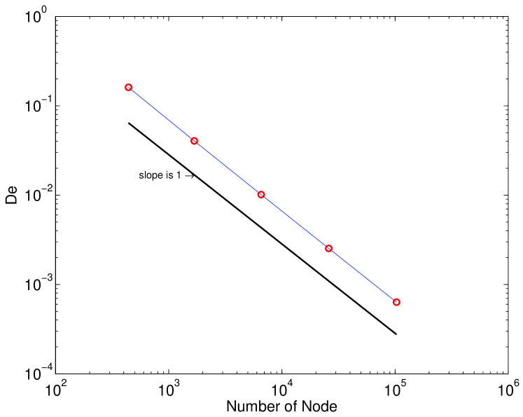
Figure 4. Linear Element: Regular Pattern

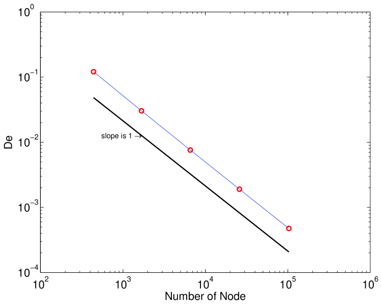
Figure 5. Linear Element: Chevron Pattern

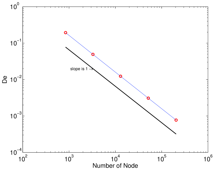
Figure 6. Linear Element: Criss-cross Pattern

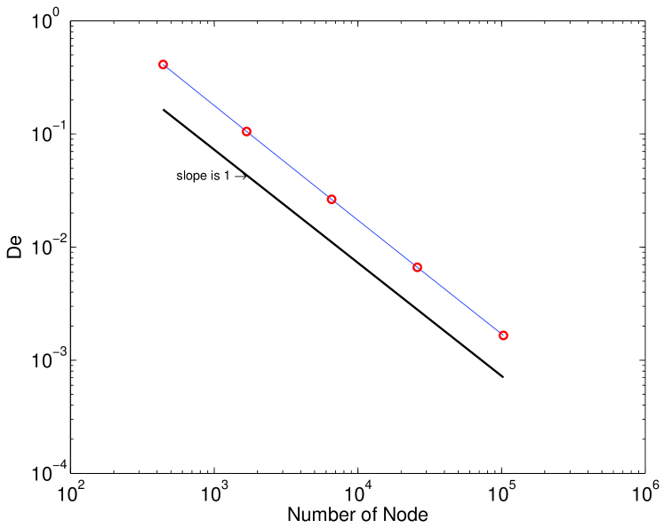
Figure 7. Linear Element: Union-Jack Pattern

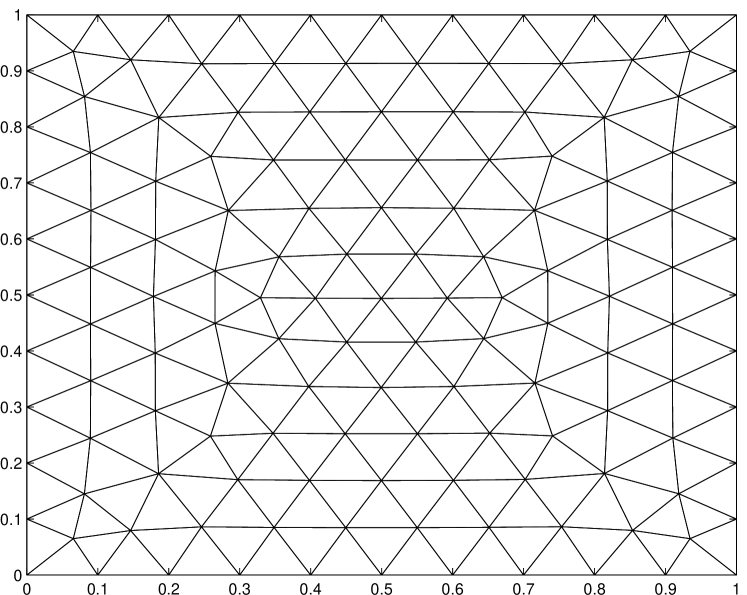
Figure 8. Delaunay

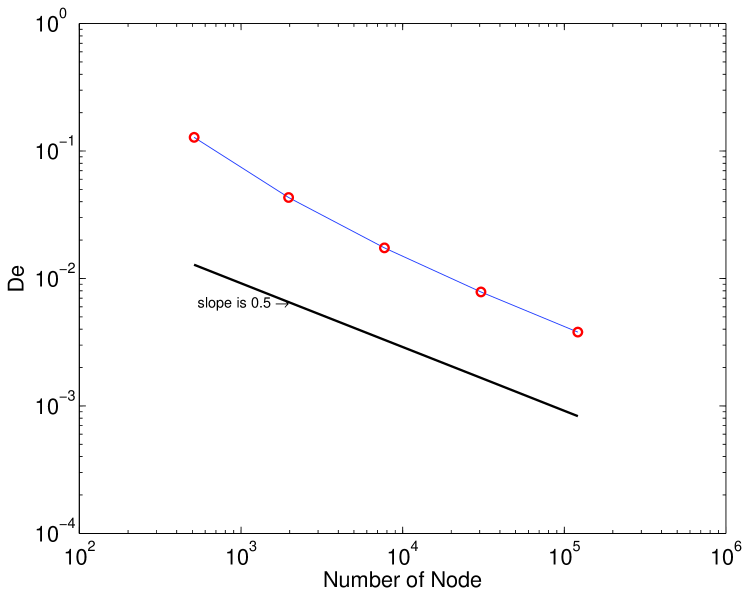
Figure 9. Linear Element: Delaunay Mesh

Then we turn to quadratic element. We test the discrete error of recovered Hessian $H_{h}u_{I}$ and the exact Hessian $Hu$ using uniform meshes of regular pattern and the same Delaunay meshes. Similarly, we define $\|\cdot\|_{\infty,h}$ as a discrete maximum norm at all vertices and edge centers in an interior region $\Omega_{1,h}$. The result of uniform mesh of regular pattern is reported in Figure 11. As predicted by Theorem 3.5, $H_{h}u_{I}$ converges to $Hu$ at rate of $O(h^{4})$ which implies $H_{h}$ preserves polynomials of degree $5$ for quadratic element on uniform triangulation. For unstructured mesh, we observe that $H_{h}u_{I}$ approximates $Hu$ at a rate of $O(h^{2})$ from Figure 11.

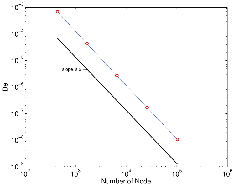
Figure 10. Quadratic Element: Regular Pattern

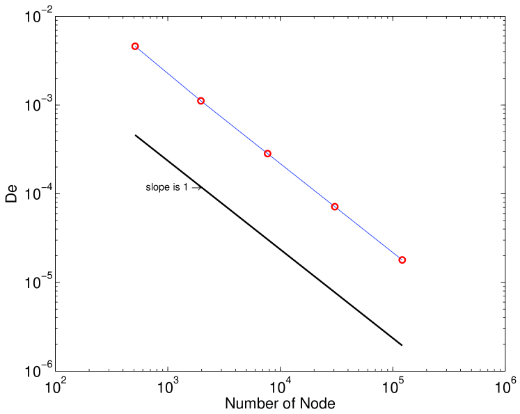
Figure 11. Quadratic Element: Delaunay Mesh

Example 2. We consider the following elliptic equation

(5.2) $$\begin{cases}-\Delta u=2\pi^{2}\sin\pi x\sin\pi y,&\text{in }\Omega=[0,1]\times[0,1],\\ u=0,&\text{on }\partial\Omega.\end{cases}$$

The exact solution is $u(x,y)=\sin(\pi x)\sin(\pi y)$. First, linear element is considered. In Table 1, we report the numerical results for regular pattern meshes. All four methods ultraconverge at a rate of $O(h^{2})$ in the interior subdomain. The fact that $H_{h}^{LS}$ and $H^{ZZ}_{h}$ perform as good as $H_{h}$ is not a surprise since it is well known that the polynomial preserving recovery is the same as weighted average for uniform triangular mesh of the regular pattern.

The results of the Chevron pattern is shown in Table 2. $H_{h}u_{h}$ approximates $Hu$ at rate $O(h^{2})$ while $H_{h}^{LS}u_{h}$, $H_{h}^{ZZ}u_{h}$ and $H_{h}^{QF}u_{h}$ approximate $Hu$ at rate $O(h)$. It is observed that our method out-performs other three Hessian recovery methods on the Chevron pattern uniform meshes. To the best of our knowledge, the proposed PPR-PPR Hessian recovery is the only method to achieve $O(h^{2})$ superconvergence for linear element under the Chevron pattern triangular mesh.

Table 1. Example 2: Regular Pattern

Dof	$De$	order	$De^{ZZ}e$	order	$De^{LS}$	order	$De^{QF}$	order
121	7.93e-001	–	9.73e-001	–	7.93e-001	–	4.01e-001	–
441	2.02e-001	1.06	2.02e-001	1.22	2.02e-001	1.06	1.03e-001	1.05
1681	5.10e-002	1.03	5.10e-002	1.03	5.10e-002	1.03	2.61e-002	1.03
6561	1.28e-002	1.02	1.28e-002	1.02	1.28e-002	1.02	6.53e-003	1.02
25921	3.20e-003	1.01	3.20e-003	1.01	3.20e-003	1.01	1.63e-003	1.01
103041	8.00e-004	1.00	8.00e-004	1.00	8.00e-004	1.00	4.08e-004	1.00

Table 2. Example 2: Chevron Pattern

Dof	$De$	order	$De^{ZZ}e$	order	$De^{LS}$	order	$De^{QF}$	order
121	6.51e-001	–	7.98e-001	–	7.82e-001	–	9.03e-001	–
441	1.34e-001	1.22	2.12e-001	1.03	2.34e-001	0.93	4.30e-001	0.57
1681	3.38e-002	1.03	7.96e-002	0.73	9.87e-002	0.64	2.11e-001	0.53
6561	8.46e-003	1.02	3.57e-002	0.59	4.68e-002	0.55	1.05e-001	0.51
25921	2.11e-003	1.01	1.73e-002	0.53	2.30e-002	0.52	5.23e-002	0.51
103041	5.29e-004	1.00	8.57e-003	0.51	1.15e-002	0.50	2.62e-002	0.50

Table 3. Example 2: Criss-cross

Dof	$De$	order	$De^{ZZ}e$	order	$De^{LS}$	order	$De^{QF}$	order
221	5.49e-001	–	3.57e-001	–	4.40e-001	–	7.14e-001	–
841	1.28e-001	1.09	8.03e-002	1.12	1.04e-001	1.08	6.17e-001	0.11
3281	3.22e-002	1.01	2.01e-002	1.02	2.62e-002	1.01	5.95e-001	0.03
12961	8.06e-003	1.01	5.04e-003	1.01	6.55e-003	1.01	5.90e-001	0.01
51521	2.02e-003	1.00	1.26e-003	1.00	1.64e-003	1.00	5.89e-001	0.00
205441	5.04e-004	1.00	3.15e-004	1.00	4.09e-004	1.00	5.88e-001	0.00

Table 4. Example 2: Unionjack Pattern

Dof	$De$	order	$De^{ZZ}e$	order	$De^{LS}$	order	$De^{QF}$	order
121	1.25e+000	–	8.40e-001	–	9.87e-001	–	1.05e+000	–
441	3.16e-001	1.06	1.77e-001	1.20	2.48e-001	1.07	6.95e-001	0.32
1681	7.96e-002	1.03	4.46e-002	1.03	6.24e-002	1.03	6.14e-001	0.09
6561	2.00e-002	1.02	1.12e-002	1.02	1.56e-002	1.02	5.95e-001	0.02
25921	5.00e-003	1.01	2.80e-003	1.01	3.91e-003	1.01	5.90e-001	0.01
103041	1.25e-003	1.00	6.99e-004	1.00	9.78e-004	1.00	5.89e-001	0.00

Table 5. Example 2: Delaunay Mesh

Dof	$De$	order	$De^{ZZ}e$	order	$De^{LS}$	order	$De^{QF}$	order
139	4.31e-001	–	4.38e-001	–	4.40e-001	–	3.26e-001	–
513	1.38e-001	0.87	2.20e-001	0.53	1.49e-001	0.83	1.79e-001	0.46
1969	5.39e-002	0.70	2.36e-001	-0.05	5.85e-002	0.69	8.88e-002	0.52
7713	2.38e-002	0.60	1.62e-001	0.28	2.55e-002	0.61	4.35e-002	0.52
30529	1.14e-002	0.54	1.13e-001	0.26	1.19e-002	0.56	2.15e-002	0.51
121473	5.59e-003	0.51	7.97e-002	0.25	5.73e-003	0.53	1.07e-002	0.51

Then the Criss-cross pattern mesh is considered and results are displayed in Table 3. An $O(h^{2})$ convergence rate is observed for our recovery method, $H^{LS}_{h}$ and $H^{ZZ}_{h}$ while no convergence rate is observed for $H^{QF}_{h}$. The results for the Union-Jack pattern mesh is very similar to the Criss-cross pattern mesh except that our recovery method superconverges at rate $O(h^{2})$ as shown in Table 4.

Now, we turn to unstructured mesh generated by EasyMesh [6] as in the previous examples. Numerical data are listed in Table 5. $H_{h}$, $H^{LS}_{h}$ and $H^{QF}_{h}$ converge at a rate of $O(h^{2})$ while $H_{h}^{ZZ}$ only converges at a rate of $O(h)$.

The results above indicate clearly that our Hessian recovery method converges at rate $O(h)$ on general Delaunay meshes, which is predicted by Theorem 4.3. On uniform meshes, we can obtain $O(h^{2})$ ultraconvergence on an interior sub-domain as predicted by Theorem 4.7.

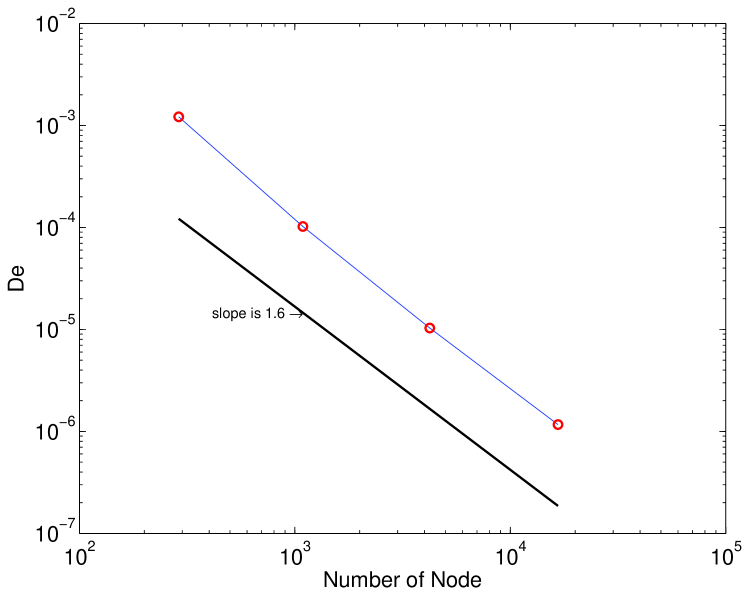
Figure 12. Example 2: Quadratic Regular Pattern

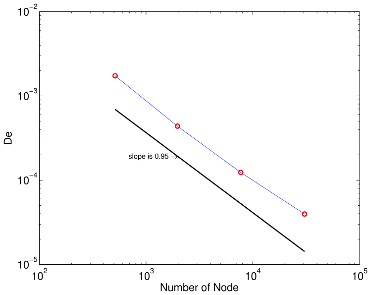
Figure 13. Example 2: Quadratic Delaunay Mesh

In the end, we consider quadratic element. Note that our Hessian recovery method is well defined for arbitrary order elements. However, the extension of the other three methods to quadratic element is not straightforward or even impossible and hence only our method is implemented here. We report the numerical results in Figure 13 for regular pattern uniform mesh. About $O(h^{3.2})$ order convergence is observed, which is a bit better than the theoretical result predicted by Theorem 4.7. Figure 13 shows the result for Delaunay mesh generated by EasyMesh [6]. About $O(h^{1.9}$ superconvergence is observed.

6. Concluding remarks

In this work, we introduced a Hessian recovery method for arbitrary order Lagrange finite elements. Theoretically, we proved that the PPR-PPR Hessian recovery operator $H_{h}$ preserves polynomials of degree $k+1$ on general unstructured meshes and preserves polynomials of degree $k+2$ on translation invariant meshes. This polynomial preserving property, combined with the supercloseness property of the finite element method, enabled us to prove convergence and superconvergence results for our Hessian recovery method on mildly structured meshes. Moreover, we proved the ultraconvergence result for translation invariant finite element space of any order by using the argument of superconvergence by difference quotient from [22].

References

- [1] A. Agouzal and Yu. Vassilevski, On a discrete Hessian recovery for finite elements, J. Numer. Math., 10(2002), 1–12.
- [2] R. E. Bank and J. Xu, Asymptotically exact a posteriori error estimators. I. Grids with superconvergence, SIAM J. Numer. Anal. 41(2003), 2294–2312.
- [3] S.C. Brenner and L.R. Scott, The mathematical theory of finite element methods, Third edition, Texts in Applied Mathematics, 15. Springer, New York, 2008.
- [4] W. Cao, Superconvergence analysis of the linear finite element method and a gradient recovery post-processing on anisotropic mesh, Math. Comp.(2013) in press.
- [5] P.G. Ciarlet, The Finite Element Method for Elliptic Problems, North-Holland, Amsterdam, 1978.
- [6] B. Niceno, EasyMesh Version 1.4: A Two-Dimensional Quality Mesh Generator, http://www-dinma.univ.trieste.it/nirftc/research/easymesh.
- [7] X. Gan and J.E. Akin, Superconvergent second order derivative recovery technique and its application in a nonlocal damage mechanics model, Finite Elements in Analysis and Design, 35(2014), 118–127.
- [8] C. Huang and Z. Zhang, Polynomial preserving recovery for quadratic elements on anisotropical meshes, Numer. Methods Partial Differential Equations, 28(2012), 966-983.
- [9] Y. Huang and J. Xu, Superconvergence of quadratic finite elements on mildly structured grids., Math. Comp., 77(2008), 1253–1268.
- [10] L. Kamenski and W. Huang, How a nonconvergent recovered Hessian works in mesh adaptation, arXiv:1211.2877v2[math.NA].
- [11] A. M. Lakhany and J. R. Whiteman Superconvergent Recovery Operators: Derivative Recovery Techniques, Finite Element Methods: Superconvergence, Post-processing, and a posteriori estimates, M. Krizek, P. Neittaanmaki, and R. Stenberg, Marcel Dekker INC, Newyork, 1998, pp. 195–216.
- [12] O. Lakkis and T. Payer, A finite element Method for second order nonvariational elliptic problems, SIAM J. Sci. Comput., 33(2011), 786–801.
- [13] O. Lakkis, Omar and T. Pryer, A finite element method for nonlinear elliptic problems, SIAM J. Sci. Comput., 35(2013), 2025–2045.
- [14] A. Naga and Z. Zhang, A posteriori error estimates based on the polynomial preserving recovery, SIAM J. Numer. Anal., 42(2004), 1780–1800.
- [15] A. Naga and Z. Zhang, The polynomial-preserving recovery for higher order finite element methods in 2D and 3D, Discrete Contin. Dyn. Syst. Ser. B 5(2005), 769–798.
- [16] M. Neilan, Finite element methods for fully nonlinear second order PDEs based on a discrete Hessian with applications to the Monge-Ampre equation, J. Comput. Appl. Math., 263(2014), 351–369.
- [17] J. A. Nitsche and A. H. Schatz, Interior estimates for Ritz-Galerkin methods, Math. Comp., 28(1974), 937–958.
- [18] J. Ovall, Function, gradient, and Hessian recovery using quadratic edge-bump functions, SIAM J. Numer. Anal. 45(2007), 1064–1080.
- [19] B. Pouliot, M. Fortin, A. Fortin and E. Chamberland, On a new edge-base gradient recovery technique, Int. J. Numer. Meth. Engng., 93(2013), 52–65.
- [20] M. Picasso, F. Alauzet, H. Borouchaki, and P. George, A numerical study of some Hessian recovery techniques on isotropic and anisotropic meshes, SIAM J. Sci. Computl., 33(2011), 1058–1076.
- [21] M.-G. Vallet, C.-M. Manole, J. Dompierre, S. Dufour, and F. Guibault, Numerical comparsion of some Hessian techniques, Internat. J. Numer. Methods Engrg., 72(2007), 987–1007.
- [22] L.B. Wahlbin, Superconvergence in Galerkin finite element methods, Lecture Notes in Mathematics, 1605, Springer-Verlag, Berkin, 1995.
- [23] H. Wu and Z. Zhang, Can we have superconvergent gradient recovery under adaptive meshes ?, SIAM J. Numer. Anal., 45(2007), 1701–1722.
- [24] J. Xu and Z. Zhang, Analysis of recovery type a posteriori error estimators for mildly structured grids, Math. Comp., 73(2004), 1139–1152.
- [25] Z. Zhang and A. Naga, A new finite element gradient recovery method: superconvergence property, SIAM J. Sci. Comput., 26(2005), 1192–1213.
- [26] O.C. Zienkiewicz and J.Z. Zhu, The superconvergent patch recovery and a posteriori error estimates. I. The recovery technique, Internat. J. Numer. Methods Engrg., 33(1992), 1331–1364.