Protein synthesis driven by dynamical stochastic transcription

Abstract

In this manuscript we propose a mathematical framework to couple transcription and translation in which mRNA production is described by a set of master equations while the dynamics of protein density is governed by a random differential equation. The coupling between the two processes is given by a stochastic perturbation whose statistics satisfies the master equations. In this approach, from the knowledge of the analytical time dependent distribution of mRNA number, we are able to calculate the dynamics of the probability density of the protein population.

1 Introduction

Stochasticity in biological processes, in particular of gene expression, has been studied, both experimentally and theoretically, at least since the pioneering work of Delbrück delbruck . Recent advances in experimental methods have enabled direct observation of stochastic features of gene expression, such as temporal fluctuations in individual cells or steady-state variations across a cell population Elowitz2002 ; OTKGO2002 ; BKCC2003 ; ROS2004 ; GPZC2005 ; CFX2006 ; YXRLX2006 , and data acquisition has experienced a huge improvement in the last decade. However, theoretical models have not yet been developed to the point of providing a comprehensive quantitative description for the dynamics of gene expression. The stationary regime has been exhaustively discussed in the literature, but studies on time dependent probability distributions are still scarce Jayaprakash2009 ; Swain2008 ; Ramos2011 .

In this paper, our main goal is to present and discuss a stochastic description for mRNA-protein dynamics. More precisely, we propose and solve a hybrid model for stochastic gene expression, consisting of a master equation (ME) coupled to a random differential equation (RDE). The ME describes the production of messenger RNA (mRNA) molecules triggered by a gene with various levels of promoter activity. The RDE governs the dynamics of protein synthesis: it is a linear ordinary differential equation randomly perturbed by the Markov jump process underlying the ME. The master equation part of the model is a particular case of a Markov process in a “random environment” CT1981 , composed by a birth-and-death process and a two-state markovian switching process, in continuous time; see PY1995 for the interpretation in the context of gene expression. Several variations of this type of model have been employed for the study of gene expression and have been extensively discussed in the literature KE2001 ; PE2004 ; Hornos2005 ; Paulsson2005 . The particular form of the master equation part used in this paper is the one analyzed in Innocentini2007 ; Innocentini2013 .

The motivations for such an approach can be justified on mathematical as well as biological grounds. From a mathematical point of view, the RDE employed here resembles a Langevin equation, with one crucial difference: the driving stochastic process is not a singular delta-like noise, but rather a non-singular, well behaved stationary stochastic process. Non-white noise driven Langevin-like equations have been widely discussed in the literature under different names, such as colored noise vKampen2007 or real noise Arnold1998 . And the mathematical advantage in dealing with RDEs is that one does not need a sophisticated theory of integration in order to solve them. As a matter of fact, RDEs are solved by Riemann integration of ordinary differential equations, sample path by sample path – hence the term “random differential equation” instead of the more familiar term “stochastic differential equation”, which is reserved for differential equations associated to a stochastic integration theory Arnold1998 .

Besides the mathematical benefit, there is a biological motivation in modeling mRNA transcription by a master equation and protein synthesis by a random differential equation, thus supposing that the transcription product should be treated as a discrete random variable (number of mRNA molecules) while the translation product should be treated as a continuous random variable (density of protein molecules). The reason behind this distinction is the large gap, typically of several orders of magnitude, between mRNA numbers and protein numbers in the cell. The hybrid model we propose here attempts to incorporate the discrepancy between mRNA and protein molecules (which concerns not only their typical numbers but also their typical lifetimes) from the very beginning, instead of assuming that it can be ignored. That is why, in conformity with procedures already adopted implicitly in some of the literature but rarely spelled out (one exception is Friedman2006 ), we suggest to model protein number by a continuous probability density rather than a discrete probability distribution.

Admittedly, this amounts to a change of paradigm, but as will be shown here, the resulting simplifications are so substantial that they allow us to solve the resulting model without constraints on the values of the parameters. Furthermore, this approach allows us to evaluate probability densities even for very high protein numbers, with no extra effort.

2 Model for Transcription and Translation

Let us describe our model in more detail. Gene transcription is described by a pair of master equations, corresponding to two states $\{1,2\}$ of promoter activity, for a birth and death process coupled by a telegraph-like process encoding the switch between promoter states (generalization to a higher number of promoter states will be left to future work):

$$\begin{split}\frac{d\phi^{1}_{n}}{dt}~{}=~{}&k_{1}[\phi^{1}_{n-1}-\phi^{1}_{n}]+\rho[(n+1)\phi^{1}_{n+1}-n\phi^{1}_{n}]-h\phi^{1}_{n}+f\phi^{2}_{n}\,,\\ \frac{d\phi^{2}_{n}}{dt}~{}=~{}&k_{2}[\phi^{2}_{n-1}-\phi^{2}_{n}]+\rho[(n+1)\phi^{2}_{n+1}-n\phi^{2}_{n}]+h\phi^{1}_{n}-f\phi^{2}_{n}\,.\end{split}$$ (1)

The discrete random variable $n$ stands for the number of mRNA molecules in the cell and $\phi^{j}_{n}(t)$ is the probability for finding the gene in state number $j$ ($j=1$ or $2$) with $n$ mRNA molecules in the cell, at time $t$; the resulting total probability will be denoted by $\phi_{n}(t)=\phi^{1}_{n}(t)+\phi^{2}_{n}(t)$. Production of mRNA is controlled by the rates $k_{1}$ and $k_{2}$, while its degradation is taken into account by the rate $\rho$ which is independent of the activity level of the promoter. The switch between the two states is controlled by the rates $h$ and $f$. Protein synthesis/degradation is governed by an RDE of the form

$$\frac{d}{dt}m_{t}\,=\,-\,Am_{t}+Bn_{t}\,,$$ (2)

where $m$ is a continuous random variable representing the protein number density in the cell, $A$ and $B$ are the protein degradation and synthesis rates, respectively, and $n$ is as before, but now with time dependence following a stochastic Markov jump process where $n_{t+\Delta t}=n_{t}\pm 1$ with probability $(k_{1}+k_{2})\Delta t$ for $+1$ and $\rho n_{t}\Delta t$ for $-1$ (and $n_{t+\Delta t}=n_{t}$ with remaining probability): this is consistent with the time evolution of the total probability distribution $\phi_{n}$ that follows from Eq. (1). With the assumption that $A$ and $B$ are constant our model focuses on the effects of the stochasticity of the transcription process and neglects the protein production/decay noise.

3 Solutions of the Model

A complete description of $n_{t}$ is achieved by obtaining the time dependent solutions of the master equations (1), and this is what we do in the following. However, before dealing with the master equations, let us first redefine the parameter space and introduce the biological quantities of the model, as in Innocentini2007 , namely: the efficiency parameters $N_{1}=k_{1}/\rho$ and $N_{2}=k_{2}/\rho$, the switching parameter $\epsilon=(h+f)/\rho$ and the occupancy probabilities $p_{1}=f/(h+f)$ and $p_{2}=h/(h+f)$. Using the generating function technique vKampen2007 the coupled master equations are transformed into a set of PDEs (partial differential equations) for the functions $\phi^{1}(z,t)=\sum^{\infty}_{n=0}\phi^{1}_{n}(t)z^{n}$ and $\phi^{2}(z,t)=\sum^{\infty}_{n=0}\phi^{2}_{n}(t)z^{n}$:

$$\begin{split}\frac{1}{\rho}\frac{\partial\phi^{1}}{\partial t}~{}=~{}&(z-1)\left[N_{1}\phi^{1}-\frac{\partial\phi^{1}}{\partial z}\right]-\epsilon p_{2}\,\phi^{1}+\epsilon p_{1}\,\phi^{2}\,,\\ \frac{1}{\rho}\frac{\partial\phi^{2}}{\partial t}~{}=~{}&(z-1)\left[N_{2}\phi^{2}-\frac{\partial\phi^{2}}{\partial z}\right]+\epsilon p_{2}\,\phi^{1}-\epsilon p_{1}\,\phi^{2}\,.\end{split}$$ (3)

The probability distributions are obtained from the generating functions using

$$\begin{split}\phi^{1}_{n}(t)~{}=~{}\left.\frac{1}{n!}\frac{\partial\phi^{1}(z,t)}{\partial z}\right|_{z=0}\,,\\ \phi^{2}_{n}(t)~{}=~{}\left.\frac{1}{n!}\frac{\partial\phi^{2}(z,t)}{\partial z}\right|_{z=0}\,,\end{split}$$ (4)

Introducing a new set of variables through the transformations $\mu=(z-1){\rm e}^{-\rho t}$ and $\nu=z-1$, Eq. (3) assumes the form

$$\begin{split}-\nu\frac{\partial\phi^{1}}{\partial\nu}+\nu N_{1}\phi^{1}-\epsilon p_{2}\,\phi^{1}+\epsilon p_{1}\,\phi^{2}&~{}=~{}0\,,\\ -\nu\frac{\partial\phi^{2}}{\partial\nu}+\nu N_{2}\phi^{2}+\epsilon p_{2}\,\phi^{1}-\epsilon p_{1}\,\phi^{2}&~{}=~{}0\,,\end{split}$$ (5)

i.e., this transformation reduces the original set of PDEs to a set of ODEs (ordinary differential equations), which have already been solved in Innocentini2007 ; a similar transformation with the same purpose has been used in Ramos2011 ; Jayaprakash2009 . Following Innocentini2007 , the solutions of Eq. (5) are:

$$\phi^{1}(\mu,\nu)~{}=~{} F(\mu)\,p_{1}\mathrm{e}^{N_{1}\nu}\operatorname{M}(a,b+1,\eta)$$ (6a)

$$-G(\mu)(1-b)\eta^{-b}\mathrm{e}^{N_{1}\nu}\operatorname{M}(a-b,1-b,\eta)\,,$$

$$\phi^{2}(\mu,\nu)~{}=~{} F(\mu)\,p_{2}\mathrm{e}^{N_{1}\nu}\operatorname{M}(a+1,b+1,\eta)$$ (6b)

$$+G(\mu)(1-b)\eta^{-b}\mathrm{e}^{N_{1}\nu}\operatorname{M}(1+a-b,1-b,\eta)\,,$$

where $F$ and $G$ are arbitrary functions that must be determined from the initial conditions, where we note that $t=0$ corresponds to $\nu=\mu$. The symbol $\operatorname{M}$ stands for the Kummer M function AandS with parameters $a=\epsilon p_{2}$, $b=\epsilon$ and $\eta=(N_{2}-N_{1})\nu$.

In order to determine $F$ and $G$ we will use matrix and vector notation to rewrite the solutions of Eq. (6) as $\vec{\phi}(\mu,\nu)=U(\nu)\vec{F}(\mu)$, where $\vec{\phi}=(\phi^{1},\phi^{2})^{\mathrm{T}}$ and $\vec{F}=(F,G)^{\mathrm{T}}$ (where $.^{\mathrm{T}}$ means matrix transposition); then the entries of the matrix $U(\nu)$ are

$$\begin{split}&U_{1,1}~{}=~{}p_{1}\,\mathrm{e}^{N_{1}\nu}\operatorname{M}(a,b+1,\eta)\,,\\[2.15277pt] &U_{1,2}~{}=~{}-(1-b)\eta^{-b}\,\mathrm{e}^{N_{1}\nu}\operatorname{M}(a-b,1-b,\eta)\,,\\[2.15277pt] &U_{2,1}~{}=~{}p_{2}\,\mathrm{e}^{N_{1}\nu}\operatorname{M}(a+1,b+1,\eta)\,,\\[2.15277pt] &U_{2,2}~{}=~{}(1-b)\eta^{-b}\,\mathrm{e}^{N_{1}\nu}\operatorname{M}(1+a-b,1-b,\eta)\,.\end{split}$$ (7)

Inverting the relation $\,\vec{\phi}(\mu,\nu)=U(\nu)\vec{F}(\mu)\,$ gives $\,\vec{F}(\mu)=U(\nu)^{-1}\vec{\phi}(\mu,\nu)$, and setting $\nu=\mu$, we obtain an expression for $\vec{F}(\mu)$ in terms of the initial conditions. Thus we have to compute the inverse of the matrix $U(\nu)$, which requires calculating its determinant. At a first glance, it might appear difficult to find a compact formula for that, since it involves products of Kummer functions. Fortunately, the well known relations for Kummer functions, especially the one concerning the Wronskian (relations 13.1.20 in AandS ), allow us to obtain a simple expression for this determinant:

$$\det(U(\nu))~{}=~{}\frac{\mathrm{e}^{-(N_{1}+N_{2})\nu}\eta^{\epsilon}}{1-\epsilon}\,.$$ (8)

Putting everything together, we obtain the time dependent probability distributions that solve Eq. (1) and will serve as input to solve Eq. (2).

Considering any given perturbation $n_{t}$ as input, the ODE (2) governing the protein dynamics is easily solved by applying the standard integral formula from the theory of ODEs. Introducing the dimensionless parameters $\tau=\rho\,t$, $\alpha=A/\rho$ and $\beta=B/\rho$, the solution reads

$$m_{\tau}~{}=~{}m_{0}\,\mathrm{e}^{-\alpha\tau}+\beta\,\mathrm{e}^{-\alpha\tau}\int_{0}^{\tau}n_{\tau^{\prime}}\,\mathrm{e}^{\alpha\tau^{\prime}}\mathrm{d}\tau^{\prime}\,,$$ (9)

where the integral is an ordinary Riemann integral (applied to the product of a step function by an exponential function) and $m_{0}=m(0)$. In the present case, where both $n_{\tau}$ and $m_{\tau}$ are stochastic processes, we can interpret this formula as an operator that maps the process $n_{\tau}$ (for mRNA number) to the process $m_{\tau}$ (for protein number density), sample by sample.

Recalling that the ultimate goal is to compute the probability density of the protein population, say $\mathscr{P}(\tau,m)$, the traditional method consists in randomly generating stochastic processes $n_{\tau}$ for mRNA number, applying the previous integral formula to produce corresponding stochastic processes $m_{\tau}$ for protein number density and looking at the resulting statistics. Here, and this is perhaps the central point of the present paper, we propose a different procedure: since the solution of Eq. (1) has already provided us with a probability distribution for mRNA number, it suffices to take its push-forward, in the sense of measure theory, under the operator defined by solving Eq. (9) to directly obtain the corresponding probability distribution for protein number density, without having to resort to random process generation. To describe how to compute the push-forward, let us consider the integral on the rhs of Eq. (9). Dividing the interval $[0,\tau]$ in $p$ subintervals we have:

$$\int_{0}^{\tau}n_{\tau^{\prime}}\,\mathrm{e}^{\alpha\tau^{\prime}}\mathrm{d}\tau^{\prime}~{}=~{}\sum_{q=0}^{p-1}\int_{\tau_{q}}^{\tau_{q+1}}n_{\tau^{\prime}}\,\mathrm{e}^{\alpha\tau^{\prime}}\mathrm{d}\tau^{\prime},$$ (10)

where $\tau_{0}=0$ and $\tau_{p}=\tau$. If the partition is sufficiently fine (i.e., for $p$ sufficiently large), the function $n_{\tau}$ will be constant on each subinterval and the integral can be performed explicitly:

$$m_{\tau}~{}=~{}m_{0}\,\mathrm{e}^{-\alpha\tau}+\frac{\beta}{\alpha}\mathrm{e}^{-\alpha\tau}\sum_{q=0}^{p-1}n_{\tau_{q}}(\mathrm{e}^{\alpha\tau_{q+1}}-\mathrm{e}^{\alpha\tau_{q}}).$$ (11)

Otherwise, i.e., for smaller values of $p$, Eq. (11) provides only a “rectangular” or “piecewise constant” approximation of the integral in Eq. (10) since it amounts to replacing, on each of the subintervals $[\tau_{q},\tau_{q+1}]$, the step function $n_{\tau^{\prime}}$ by a constant (here chosen to be its value at the left endpoint):

$$\int_{\tau_{q}}^{\tau_{q+1}}n_{\tau^{\prime}}\,\mathrm{e}^{\alpha\tau^{\prime}}\mathrm{d}\tau^{\prime}\approx n_{\tau_{q}}\int_{\tau_{q}}^{\tau_{q+1}}\mathrm{e}^{\alpha\tau^{\prime}}\mathrm{d}\tau^{\prime}~{}=~{}\frac{n_{\tau_{q}}}{\alpha}\,\bigg{|}_{\tau_{q}}^{\tau_{q+1}}.$$ (12)

Of course, a “trapezoidal” or “piecewise linear” approximation is more precise: it consists in replacing this expression by

$$\int_{\tau_{q}}^{\tau_{q+1}}n_{\tau^{\prime}}\,\mathrm{e}^{\alpha\tau^{\prime}}\mathrm{d}\tau^{\prime}\approx\int_{\tau_{q}}^{\tau_{q+1}}(a\tau^{\prime}+b)\,\mathrm{e}^{\alpha\tau^{\prime}}\mathrm{d}\tau^{\prime}=\frac{1}{\alpha}\,(a\tau^{\prime}+b-\frac{a}{\alpha})\,\mathrm{e}^{\alpha\tau^{\prime}}\,\bigg{|}_{\tau_{q}}^{\tau_{q+1}},$$ (13)

where $a$ and $b$ are determined by solving the equations $\,n_{\tau_{q}}=a\tau_{q}+b\,$ and $\,n_{\tau_{q+1}}=a\tau_{q+1}+b$.

In order to obtain a sample path for the process $m_{\tau}$ using these formulas, it suffices to represent a sample path for the process $n_{\tau}$ by the “shrunk” numerical sequence $(n_{0},\ldots,n_{p-1})$, the only modification being that we must now allow consecutive numbers to differ by more than $\pm 1$. Finally, to make our sample space finite, we also introduce a cutoff $L$ and impose that all $n_{q}$ should be $\leqslant L$. For instance, by choosing $L$ so large that the probability of $n_{q}>L$ is smaller than $10^{-20}$, say, we can certainly neglect all values higher than $L$ and restrict the set of possible values for $n_{q}$ to the finite set $\{0,1,\ldots,L-1,L\}$; then the space of sequences has $(L+1)^{p}$ elements.

Now, Eq. (11) provides a map from this space of sequences $(n_{0},\ldots,n_{p-1})$ to that of numbers $m_{\tau}$. Using this mapping we define the push-forward probability on the set of possible values of $m_{\tau}$ by

$$\mathbf{P}\bigl{(}m_{\tau}=m_{\tau}(n_{0},\ldots,n_{p-1})\bigr{)}=\Phi(n_{0};\ldots;n_{p-1}),$$ (14)

where

$$\Phi(n_{0};\ldots;n_{p-1})=\Phi^{1}(n_{0};\ldots;n_{p-1})+\Phi^{2}(n_{0};\ldots;n_{p-1})$$ (15)

is the total joint probability distribution for finding $n_{q}$ mRNA molecules at times $\tau_{q}$ $(q=0,\ldots,p-1)$, whereas $\Phi^{1}(n_{0};\ldots;n_{p-1})$ and $\Phi^{2}(n_{0};\ldots;n_{p-1})$ encode the joint probability distributions for finding $n_{q}$ mRNA molecules at times $\tau_{q}$ $(q=0,...,p-1)$ with the gene in promoter state $1$ and $2$, respectively. In general, such joint probability distributions are difficult to obtain, but in our case, the mRNA process governed by the master equations (1) is markovian and therefore we can compute the joint probabilities in terms of conditional probabilities, according to the iterated Chapman-Kolmogorov equation:

$$\begin{split}\Phi^{1}(n_{0};\ldots;n_{p-1})=\sum_{j_{0},\ldots,j_{p-2}=1}^{2}&\Phi(n_{p-1},\tau_{p-1},1|n_{p-2},\tau_{p-2},j_{p-2})\ldots\\[-4.30554pt] &\ldots\Phi(n_{1},\tau_{1},j_{1}|n_{0},\tau_{0},j_{0})\,\phi_{n_{0}}^{j_{0}}(\tau_{0})\,,\\ \Phi^{2}(n_{0};\ldots;n_{p-1})=\sum_{j_{0},\ldots,j_{p-2}=1}^{2}&\Phi(n_{p-1},\tau_{p-1},2|n_{p-2},\tau_{p-2},j_{p-2})\ldots\\[-4.30554pt] &\ldots\Phi(n_{1},\tau_{1},j_{1}|n_{0},\tau_{0},j_{0})\,\phi_{n_{0}}^{j_{0}}(\tau_{0})\,,\end{split}$$ (16)

where, as before, $\phi_{n_{0}}^{j_{0}}(\tau_{0})$ is the probability to find the gene in the state $j_{0}$ and with $n_{0}$ mRNA molecules in the cell, at time $\tau_{0}$. The quantity $\Phi(n_{q^{\prime}},\tau_{q^{\prime}},j^{\prime}|n_{q},\tau_{q},j)$ is the conditional probability of finding $n_{q^{\prime}}$ mRNA molecules at time $\tau_{q^{\prime}}$ and with the gene in state $j^{\prime}$ provided there were $n_{q}$ mRNA molecules at time $\tau_{q}$ and with the gene in state $j$, where $\tau_{q}<\tau_{q^{\prime}}$, $q,q^{\prime}=1,\ldots,p-1$ and $j,j^{\prime}=1,2$. These conditional probabilities can be obtained from the solutions of the master equations (6). To this end, one has to take as initial condition the generating function encoding the information that, at time $\tau_{q}$, the system has exactly $n_{q}$ particles and with probability $1$ is in one of the two promoter states, say 1 or 2. Such a generating function has one component equal to $0$ whereas the other is given by $(1+\mu)^{n_{q}}$, i.e.,

$$(\phi^{1}(\mu,\nu),\phi^{2}(\mu,\nu))=([1+\mu]^{q},0)\quad\mbox{with}\quad\nu=\mu$$ (17)

for promoter in state $1$ and

$$(\phi^{1}(\mu,\nu),\phi^{2}(\mu,\nu))=(0,[1+\mu]^{q})\quad\mbox{with}\quad\nu=\mu$$ (18)

for promoter in state $2$. In the $(z,\tau)$ variables, the non-vanishing component takes the form

$$\left(1+(z-1)\mathrm{e}^{-(\tau-\tau_{q})}\right)^{n_{q}}$$ (19)

since here the initial time is $\tau_{q}$, rather than $0$.

Regarding the validity of Eq. (14), it is important to note that according to the general definition of the push-forward of probabilities, one should really take the sum of the probabilities corresponding to all sequences $(n_{0},\ldots,n_{p-1})$ producing the same value of $m_{\tau}$. However, Eq. (11) implies that, generically, any two different sequences will give different values (more precisely, this will be the case if the intermediate times $\tau_{1},\ldots,\tau_{p-1}$ are chosen such that the differences of exponentials $\,\mathrm{e}^{\alpha\tau_{q+1}}-\mathrm{e}^{\alpha\tau_{q}}$, $q=0,\ldots,p-1$, are linearly independent over the integers).

For the sake of greater clarity, and to illustrate how the conditional probabilities are obtained from the explicit solution (6) of the master equations with the appropriate initial conditions (see Eqs (17),(18) and (19) above), let us consider the simplest example: $p=2$ and $L=1$. Here, the sample space has four elements, namely, $(0,0)$, $(0,1)$, $(1,0)$ and $(1,1)$, and in general each of these sequences will produce a different number $m_{\tau}$. Therefore, the probability assigned to each of these values $m_{\tau}$ is equal to the joint probability assigned to the corresponding sequence $(n_{0},n_{1})$, summed over the two possible promoter states,

$$\mathbf{P}(m_{\tau}=m_{\tau}(n_{0},n_{1}))=\Phi^{1}(n_{0};n_{1})+\Phi^{2}(n_{0};n_{1}).$$ (20)

Specializing Eq. (16) to the case $p=2$, we see that these joint probabilities are

$$\begin{array}[]{c}\Phi^{1}(n_{0};n_{1})=\Phi(n_{1},\tau_{1},1|n_{0},\tau_{0},1)\,\phi^{1}_{n_{0}}(\tau_{0})+\Phi(n_{1},\tau_{1},1|n_{0},\tau_{0},2)\,\phi^{2}_{n_{0}}(\tau_{0})\,,\\[4.30554pt] \Phi^{2}(n_{0};n_{1})=\Phi(n_{1},\tau_{1},2|n_{0},\tau_{0},1)\,\phi^{1}_{n_{0}}(\tau_{0})+\Phi(n_{1},\tau_{1},2|n_{0},\tau_{0},2)\,\phi^{2}_{n_{0}}(\tau_{0})\,,\end{array}$$ (21)

where, as before, the conditional probabilities $\Phi(n_{1},\tau_{1},j_{1}|n_{0},\tau_{0},j_{0})$ take into account the promoter states. To exemplify how these are obtained from the solutions of the master equations, let us, by way of example, focus on the conditional probability $\Phi(n_{1}=5,\tau_{1},j_{1}=1|n_{0}=10,\tau_{0},j_{0}=1)$. This means that we are considering the situation where, at time $\tau_{0}$, the system has 10 mRNA molecules and the promoter is found in the state 1, corresponding to the initial condition

$$(\phi^{1}(\mu,\nu),\phi^{2}(\mu,\nu))=([1+\mu]^{10},0)\quad\mbox{with}\quad\nu=\mu,$$ (22)

or in the $(z,\tau)$ variables,

$$(\phi^{1}(z,\tau_{1}),\phi^{2}(z,\tau_{1}))=\left(\left[1+(z-1)\,\mathrm{e}^{-(\tau_{1}-\tau_{0})}\right]^{10},0\right).$$ (23)

Using Eq. (22) to determine the vector

$$\vec{F}(\mu)=U(\nu)^{-1}\vec{\phi}(\mu,\nu)\Bigr{|}_{\nu=\mu},$$ (24)

substituting the entries of this vector in Eq. (6a) for $\phi^{1}$ and returning to the variables $(z,\tau)$, we arrive at the generating function, let’s say $\Psi(z,\tau)$, of the conditional probabilities $\Phi(n_{1},\tau_{1},j_{1}=1|n_{0}=10,\tau_{0},j_{0}=1)$, from which the conditional probability under consideration can be obtained by taking derivatives, as follows:

$$\Phi(n_{1}=5,\tau_{1},j_{1}=1|n_{0}=10,\tau_{0},j_{0}=1)=\frac{1}{5!}\frac{\partial^{5}\Psi(z,\tau)}{\partial z^{5}}\Bigr{|}_{z=0}.$$ (25)

When the system at initial time $\tau_{0}$ is in promoter state 2 rather than 1, we have to switch the two components in the vector of Eqs (22) and (23), use the entries of this vector to determine $\vec{F}$, according to Eq. (24), and again apply Eq. (6a) for $\phi^{1}$ to obtain the generating function for the conditional probability $\Phi(n_{1}=5,\tau_{1},j_{1}=1|n_{0}=10,\tau_{0},j_{0}=2)$. And finally, to compute the conditional probabilities $\Phi(n_{1}=5,\tau_{1},j_{1}=2|n_{0}=10,\tau_{0},j_{0})$, with $j_{0}=1\,\mbox{or}\,2$, we proceed in the same way, the only difference being that instead of using Eq. (6a) for $\phi^{1}$ we use Eq. (6b) for $\phi^{2}$.

From Eq. (14) the probability density for protein number is obtained as the limit

$$\mathscr{P}(\tau,m)=\lim_{L,p\to\infty}\mathbf{P}(m_{\tau}(n_{0},\ldots,n_{p-1})),$$ (26)

where $\tau_{q+1}-\tau_{q}\to 0$ as $p\to\infty$ in such a way that the product $p\,(\tau_{q+1}-\tau_{q})$ remains finite. The computational implementation of this limit is obtained by approximating the probability density by a histogram.

Finally, to consider arbitrarily long times, we take advantage of the fact that Eq. (2) is autonomous and hence its solutions have a composition property, namely:

$$m_{\tau,\tau}=\operatorname{id}\quad,\qquad m_{\tau,\tau^{\prime}}\circ m_{\tau^{\prime},\tau^{\prime\prime}}=m_{\tau,\tau^{\prime\prime}}\,.$$ (27)

These formulas are obtained from the general solution of the initial value problem with $m(\tau^{\prime})=m_{\tau^{\prime}}$ ($\tau^{\prime}<\tau$),

$$m_{\tau,\tau^{\prime}}=m_{\tau^{\prime}}\,\mathrm{e}^{-\alpha(\tau-\tau^{\prime})}+\beta\int_{\tau^{\prime}}^{\tau}n_{\tau^{\prime\prime}}\,\mathrm{e}^{-\alpha(\tau-\tau^{\prime\prime})}\mathrm{d}\tau^{\prime\prime},$$ (28)

which defines a family of transformations acting on the set of initial conditions. By iteration, it follows that the solution may be written as $m_{\tau}=m_{\tau_{p},\tau_{p-1}}\circ\cdots\circ m_{\tau_{1},\tau_{0}}$, where $\{\tau_{0}=0,\ldots,\tau_{p}=\tau\}$ is any subdivision of the time interval $[0,\tau]$ and each $m_{\tau_{q+1},\tau_{q}}$ is given by Eq. (28), with the initial condition $m(\tau_{q})=m_{\tau_{q}}$ having probability density $\mathscr{P}(\tau_{q},m)$, for $q=0,\ldots,p-1$.

4 Moments of mRNA number and protein number distribution

The time dependent mRNA moments can be obtained directly from the solutions of Eqs (5) given in Eqs (6), by transforming back to the original $(z,\tau)$ variables and taking derivatives of these generating functions with respect to the variable $z$ at $z=1$:

$$\langle n^{(r)}_{\tau}\rangle_{j}=\left(z\frac{\partial}{\partial z}\right)^{\!r}\phi^{j}(z,\tau)\Big{|}_{z=1}\quad(j=1,2).$$ (29)

Alternatively, we can view each of these moments as the solution of its own system of ordinary differential equations, obtained by applying the operator $(z\,\partial/\partial z)^{r}|_{z=1}$ directly to the system of partial differential equations (3), rather than its solutions. This is the procedure we shall adopt in what follows, for the first two moments.

As a preliminary step, we note that taking $r=0$ (which amounts to simply evaluating Eq. (3) at $z=1$) gives, for the promoter state occupancy probabilities

$$\pi_{j}(\tau)=\sum_{n\geq 0}\phi_{n}^{j}(\tau)=\phi^{j}(\tau,z=1)\quad(j=1,2),$$ (30)

the following system of differential equations,

$$\begin{array}[]{c}{\displaystyle\frac{\mathrm{d}}{\mathrm{d}\tau}{\pi_{1}}=-\,\epsilon p_{2}\,\pi_{1}+\epsilon p_{1}\,\pi_{2}}\,,\\[8.61108pt] {\displaystyle\frac{\mathrm{d}}{\mathrm{d}\tau}{\pi_{2}}=\epsilon p_{2}\,\pi_{1}-\epsilon p_{1}\,\pi_{2}}\,.\end{array}$$ (31)

Its solution is immediate,

$$\begin{array}[]{c}\pi_{1}(\tau)=p_{1}+(\pi_{1}(0)-p_{1})\,\mathrm{e}^{-\epsilon\tau},\\[4.30554pt] \pi_{2}(\tau)=p_{2}+(\pi_{2}(0)-p_{2})\,\mathrm{e}^{-\epsilon\tau},\end{array}$$ (32)

provided we take into account that $p_{1}+p_{2}=1$: this will imply that the constraint $\,\pi_{1}(\tau)+\pi_{2}(\tau)=1\,$ is conserved (it holds for all $\tau$ provided it holds for the initial condition, i.e., for $\tau=0$) and allow us to interpret the coefficients $p_{j}$ as the asymptotic promoter state occupancy probabilities:

$$p_{j}=\lim_{\tau\to\infty}\pi_{j}(\tau)\quad(j=1,2).$$ (33)

4.1 Mean values

Considering the case $r=1$, we apply the operator $(z\,\partial/\partial z)$ to Eqs (3) and evaluate at $z=1$ to obtain, for the mean partial mRNA numbers

$$\langle n_{\tau}^{(1)}\rangle_{j}=\sum_{n\geq 0}n\,\phi_{n}^{j}(\tau)=\Bigl{(}z\frac{\partial}{\partial z}\Bigr{)}\phi^{j}(z,\tau)\Big{|}_{z=1}\quad(j=1,2),$$ (34)

the following system of differential equations,

$$\begin{array}[]{c}\dfrac{\mathrm{d}}{\mathrm{d}\tau}\langle n^{(1)}_{\tau}\rangle_{1}=-(1+\epsilon p_{2})\langle n^{(1)}_{\tau}\rangle_{1}+\epsilon p_{1}\langle n^{(1)}_{\tau}\rangle_{2}+N_{1}\pi_{1}(\tau)\,,\\[8.61108pt] \dfrac{\mathrm{d}}{\mathrm{d}\tau}\langle n^{(1)}_{\tau}\rangle_{2}=-(1+\epsilon p_{1})\langle n^{(1)}_{\tau}\rangle_{2}+\epsilon p_{2}\langle n^{(1)}_{\tau}\rangle_{1}+N_{2}\pi_{2}(\tau)\,.\end{array}$$ (35)

The corresponding differential equation for the mean total mRNA number

$$\langle n_{\tau}^{(1)}\rangle=\langle n_{\tau}^{(1)}\rangle_{1}+\langle n_{\tau}^{(1)}\rangle_{2}$$ (36)

is obtained by summing over $j$:

$$\dfrac{\mathrm{d}}{\mathrm{d}\tau}\langle n_{\tau}^{(1)}\rangle=-\langle n_{\tau}^{(1)}\rangle+N_{1}\pi_{1}(\tau)+N_{2}\pi_{2}(\tau)\,.$$ (37)

Note that we can solve this equation without having to solve the full system (35). Namely, introducing the constants

$$\bar{N}=N_{1}p_{1}+N_{2}p_{2}\quad,\quad\Delta N=N_{1}-N_{2}\,,$$ (38)

we get from Eq. (32)

$$N_{1}\pi_{1}(\tau)+N_{2}\pi_{2}(\tau)=\bar{N}+\Delta N\,(\pi_{1}(0)-p_{1})\,\mathrm{e}^{-\epsilon\tau},$$

and this can be used to integrate Eq. (37), after putting it in the form

$$\mathrm{e}^{-\tau}\frac{\mathrm{d}}{\mathrm{d}\tau}{\bigl{(}\mathrm{e}^{\tau}\langle n^{(1)}_{\tau}\rangle\bigr{)}}=N_{1}\pi_{1}(\tau)+N_{2}\pi_{2}(\tau)\,.$$

The solution is

$$\langle n^{(1)}_{\tau}\rangle=\bar{N}+(\langle n^{(1)}_{0}\rangle-\bar{N})\,\mathrm{e}^{-\tau}+\frac{\Delta N}{1-\epsilon}\bigl{(}\pi_{1}(0)-p_{1}\bigr{)}\bigl{(}\mathrm{e}^{-\epsilon\tau}-\mathrm{e}^{-\tau}\bigr{)}\,,$$ (39)

with the asymptotic value

$$\langle n^{(1)}_{\infty}\rangle=\lim_{\tau\to\infty}\langle n^{(1)}_{\tau}\rangle=\bar{N}\,.$$ (40)

For later use, we record here the complete solution of the system (35) because it will be needed at the next stage; it reads

$$\begin{split}\langle n^{(1)}_{\tau}\rangle_{1}=\;&\langle n^{(1)}_{\infty}\rangle_{1}+\frac{\epsilon\,\Delta N\,p_{1}(\pi_{1}(0)-p_{1})}{1-\epsilon}\,\mathrm{e}^{-\tau}\\ &+\frac{[\epsilon(\Delta N\,p_{1}-N_{1})+N_{1}](\pi_{1}(0)-p_{1})}{1-\epsilon}\,\mathrm{e}^{-\epsilon\tau}\\ &-\frac{\epsilon\,\Delta N(\pi_{1}(0)-p_{1})(\pi_{2}(0)-p_{1})}{1+\epsilon}\,\mathrm{e}^{-(1+\epsilon)\tau}\end{split}$$ (41)

for the partial mean value when the gene is in the state 1, and

$$\begin{split}\langle n^{(1)}_{\tau}\rangle_{2}=\;&\langle n^{(1)}_{\infty}\rangle_{2}+\frac{\epsilon\,\Delta N\,p_{2}(\pi_{1}(0)\!-\!p_{1})}{1-\epsilon}\,\mathrm{e}^{-\tau}\\ &-\frac{[\epsilon(\Delta N\,p_{1}-N_{1})+N_{2}](\pi_{1}(0)-p_{1})}{1-\epsilon}\,\mathrm{e}^{-\epsilon\tau}\\ &+\frac{\epsilon\,\Delta N(\pi_{1}(0)-p_{1})(\pi_{2}(0)-p_{1})}{1+\epsilon}\,\mathrm{e}^{-(1+\epsilon)\tau}\end{split}$$ (42)

for the partial mean value when the gene is in the state 2, with the asymptotic values

$$\langle n^{(1)}_{\infty}\rangle_{1}=N_{1}p_{1}+\frac{\epsilon N_{2}p_{2}}{1+\epsilon}\quad,\quad\langle n^{(1)}_{\infty}\rangle_{2}=N_{2}p_{2}+\frac{\epsilon N_{1}p_{1}}{1+\epsilon}\,.$$ (43)

The ordinary differential equation governing the mean protein number density is obtained by averaging Eq. (2) which, in terms of the rescaled variables, gives

$$\dfrac{\mathrm{d}}{\mathrm{d}\tau}\langle m_{\tau}\rangle=-\,\alpha\,\langle m_{\tau}\rangle+\beta\,\langle n^{(1)}_{\tau}\rangle.$$ (44)

The solution of this equation is as in Eq. (9):

$$\langle m_{\tau}\rangle=\langle m_{0}\rangle\,\mathrm{e}^{-\alpha\tau}+\beta\,\mathrm{e}^{-\alpha\tau}\int_{0}^{\tau}\langle n^{(1)}_{\tau^{\prime}}\rangle\,\mathrm{e}^{\alpha\tau^{\prime}}\mathrm{d}\tau^{\prime}.$$ (45)

Using Eqs (39) and (45), we integrate this to find

$$\begin{split}\langle m_{\tau}\rangle~{}=&~{}\langle m_{0}\rangle\,\mathrm{e}^{-\alpha\tau}+\bar{N}\frac{\beta}{\alpha}(1-\mathrm{e}^{-\alpha\tau})+\beta(\langle n^{(1)}_{0}\rangle-\bar{N})\left(\frac{\mathrm{e}^{-\tau}-\mathrm{e}^{-\alpha\tau}}{\alpha-1}\right)\\ &~{}+\Delta N\frac{\beta}{1-\epsilon}(\pi_{1}(0)-p_{1})\left(\frac{\mathrm{e}^{-\epsilon\tau}-\mathrm{e}^{-\alpha\tau}}{\alpha-\epsilon}-\frac{\mathrm{e}^{-\tau}-\mathrm{e}^{-\alpha\tau}}{\alpha-1}\right).\end{split}$$ (46)

with the asymptotic value

$$\langle m_{\infty}\rangle=\lim_{\tau\to\infty}\langle m_{\tau}\rangle=\bar{N}\frac{\beta}{\alpha}\,.$$ (47)

4.2 Variance

Passing to the case $r=2$, we apply the operator $(z\,\partial/\partial z)$ to Eqs (3) twice and evaluate at $z=1$ to obtain, for the partial second moments

$$\langle n_{\tau}^{(2)}\rangle_{j}=\sum_{n\geq 0}n^{2}\,\phi_{n}^{j}(\tau)=\Bigl{(}z\frac{\partial}{\partial z}\Bigr{)}^{\!2}\phi^{j}(z,\tau)\Big{|}_{z=1}\quad(j=1,2),$$ (48)

the following system of ordinary differential equations,

$$\begin{array}[]{c}\dfrac{\mathrm{d}}{\mathrm{d}\tau}\langle n^{(2)}_{\tau}\rangle_{1}=-\,2\langle n^{(2)}_{\tau}\rangle_{1}+(2N_{1}+1-\epsilon p_{2})\langle n^{(1)}_{\tau}\rangle_{1}+\epsilon p_{1}\langle n^{(1)}_{\tau}\rangle_{2}+N_{1}\pi_{1}(\tau),\\[8.61108pt] \dfrac{\mathrm{d}}{\mathrm{d}\tau}\langle n^{(2)}_{\tau}\rangle_{2}=-\,2\langle n^{(2)}_{\tau}\rangle_{2}+(2N_{2}+1-\epsilon p_{1})\langle n^{(1)}_{\tau}\rangle_{2}+\epsilon p_{2}\langle n^{(1)}_{\tau}\rangle_{1}+N_{2}\pi_{2}(\tau).\end{array}$$ (49)

The corresponding differential equation for the total second moment

$$\langle n_{\tau}^{(2)}\rangle=\langle n_{\tau}^{(2)}\rangle_{1}+\langle n_{\tau}^{(2)}\rangle_{2}$$ (50)

is obtained by summing over $j$:

$$\dfrac{\mathrm{d}}{\mathrm{d}\tau}\langle n_{\tau}^{(2)}\rangle=-\,2\langle n^{(2)}_{\tau}\rangle+(2N_{1}+1)\langle n^{(1)}_{\tau}\rangle_{1}+(2N_{2}+1)\langle n^{(1)}_{\tau}\rangle_{2}+N_{1}\pi_{1}(\tau)+N_{2}\pi_{2}(\tau).$$ (51)

Equivalently, we can derive a differential equation directly for the variance

$$V(n_{\tau})=\langle n^{(2)}_{\tau}\rangle-\langle n^{(1)}_{\tau}\rangle^{2}$$ (52)

by using Eq. (37) to deduce that

$$\dfrac{\mathrm{d}}{\mathrm{d}\tau}\langle n^{(1)}_{\tau}\rangle^{2}=2\langle n^{(1)}_{\tau}\rangle\,\dfrac{\mathrm{d}}{\mathrm{d}\tau}\langle n^{(1)}_{\tau}\rangle=-2\langle n^{(1)}_{\tau}\rangle^{2}+2\langle n^{(1)}_{\tau}\rangle(N_{1}\pi_{1}(\tau)+N_{2}\pi_{2}(\tau))$$

and subtracting this result from Eq. (51) to arrive at

$$\begin{split}\dfrac{\mathrm{d}}{\mathrm{d}\tau}V(n_{\tau})=\;&-2V(n_{\tau})+\langle n^{(1)}_{\tau}\rangle[1-2(N_{1}\pi_{1}(\tau)+N_{2}\pi_{2}(\tau))]\\ &+2N_{1}\langle n^{(1)}_{\tau}\rangle_{1}+2N_{2}\langle n^{(1)}_{\tau}\rangle_{2}+N_{1}\pi_{1}(\tau)+N_{2}\pi_{2}(\tau).\end{split}$$ (53)

Again, we can solve Eqs (51) and (53) without having to solve the full system (49), but here we now need the full solution of the system (35), Eqs (41) and (42). For the variance, this solution has the following structure:

$$V(n_{\tau})=A_{1}+B_{1}\mathrm{e}^{-\tau}+C_{1}\mathrm{e}^{-2\tau}+D_{1}\mathrm{e}^{-\epsilon\tau}+E_{1}\mathrm{e}^{-(1+\epsilon)\tau}+F_{1}\mathrm{e}^{-2\epsilon\tau},$$ (54)

with coefficients given by:

$$\begin{array}[]{c}{\displaystyle A_{1}=\bar{N}+\frac{(\Delta N)^{2}\,p_{1}(1-p_{1})}{1+\epsilon}\,,}\\[12.91663pt] {\displaystyle B_{1}=-\,\frac{\epsilon\,\Delta N\,(\pi_{1}(0)-p_{1})}{1-\epsilon}\,,}\\[12.91663pt] {\displaystyle C_{1}=-\,\frac{\epsilon\,(\Delta N)^{2}\,(\pi_{1}(0)-p_{1})\,[2\pi_{1}(0)-\epsilon(\pi_{1}(0)-p_{2})-1]}{(1-\epsilon)^{2}(2-\epsilon)}\,,}\\[12.91663pt] {\displaystyle D_{1}=\Delta N\,(\pi_{1}(0)-p_{1})\left[\frac{1}{1-\epsilon}+\frac{2\,\Delta N\,(1-2p_{1})}{2-\epsilon}\right]\,,}\\[12.91663pt] {\displaystyle E_{1}=\frac{2\,\epsilon\,(\Delta N)^{2}\,(\pi_{1}(0)-p_{1})\,[2\pi_{1}(0)-\epsilon(1-2p_{1})-1]}{(1+\epsilon)(1-\epsilon)^{2}}\,,}\\[12.91663pt] {\displaystyle F_{1}=-\,\frac{(\Delta N)^{2}\,(\pi_{1}(0)-p_{1})^{2}}{(1-\epsilon)^{2}}\,.}\end{array}$$ (55)

Our final goal will be to analyze the variance of the protein number density,

$$V(m_{\tau})=\langle m^{2}_{\tau}\rangle-\langle m_{\tau}\rangle^{2}\,.$$ (56)

Using the solution for $\langle m_{\tau}\rangle$ in its integral representation, Eq. (45), the expression for $\langle m_{\tau}\rangle^{2}$ is

$$\begin{split}\langle m_{\tau}\rangle^{2}=\;&\langle m_{0}\rangle^{2}\,\mathrm{e}^{-2\alpha\tau}+2\beta\,\mathrm{e}^{-2\alpha\tau}\int_{0}^{\tau}\langle m_{0}\rangle\langle n^{(1)}_{\tau^{\prime}}\rangle\,\mathrm{e}^{\alpha\tau^{\prime}}d\tau^{\prime}\\ &+\beta^{2}\mathrm{e}^{-2\alpha\tau}\int_{0}^{\tau}\int_{0}^{\tau}\langle n^{(1)}_{\tau^{\prime}}\rangle\langle n^{(1)}_{\tau^{\prime\prime}}\rangle\,\mathrm{e}^{\alpha(\tau^{\prime}+\tau^{\prime\prime})}d\tau^{\prime}d\tau^{\prime\prime}.\end{split}$$ (57)

The expression for $\langle m^{2}_{\tau}\rangle$ is obtained by first squaring Eq. (9) and then averaging, leading to:

$$\begin{split}\langle m^{2}_{\tau}\rangle=\;&\langle m^{2}_{0}\rangle\,\mathrm{e}^{-2\alpha\tau}+2\beta\,\mathrm{e}^{-\alpha\tau}\int_{0}^{\tau}\langle m_{0}\,n_{\tau^{\prime}}\rangle\,\mathrm{e}^{\alpha\tau^{\prime}}d\tau^{\prime}\\ &+\beta^{2}\mathrm{e}^{-2\alpha\tau}\int_{0}^{\tau}\int_{0}^{\tau}\langle n_{\tau^{\prime}}n_{\tau^{\prime\prime}}\rangle\,\mathrm{e}^{\alpha(\tau^{\prime}+\tau^{\prime\prime})}d\tau^{\prime}d\tau^{\prime\prime}.\end{split}$$ (58)

With these expressions at hand and in view of the fact that $\langle m_{0}n_{\tau}\rangle=\langle m_{0}\rangle\langle n^{(1)}_{\tau}\rangle$, which means that the initial condition $m_{0}$ for protein number is independent of the mRNA process $n_{\tau}$, we arrive at an explicit expression for the variance of protein number:

$$V(m_{\tau})=\mathrm{e}^{-2\alpha\tau}\left[V(m_{0})+\beta^{2}\underbrace{\int_{0}^{\tau}\int_{0}^{\tau}\mathrm{e}^{\alpha(s+s^{\prime})}\bigl{(}\langle n_{s}n_{s^{\prime}}\rangle-\langle n^{(1)}_{s}\rangle\langle n^{(1)}_{s^{\prime}}\rangle)\,ds\,ds^{\prime}}_{I_{\tau}}\right],$$ (59)

where $\langle n_{s}n_{s^{\prime}}\rangle$ is the mRNA correlation function. Using the tower property of the conditional expectation and the Markov property of the solution of the master equation, we get, for $s>s^{\prime}$

$$\begin{split}\langle n_{s}n_{s^{\prime}}\rangle&=\sum_{n^{\prime}}\sum_{n}\sum_{j}n\,n^{\prime}\,\Phi^{j}(n^{\prime},s^{\prime};n,s)\\ &=\sum_{n^{\prime},j^{\prime}}n^{\prime}\left[\sum_{n,j}n\,\Phi(n,s,j|n^{\prime},s^{\prime},j^{\prime})\right]\,\phi_{n^{\prime}}^{j^{\prime}}(s^{\prime})\\ &=\sum_{n^{\prime},j^{\prime}}n^{\prime}\,\langle n_{s-s^{\prime}}^{(1)}\rangle_{n^{\prime},j^{\prime}}^{\vphantom{(1)}}\,\phi_{n^{\prime}}^{j^{\prime}}(s^{\prime})\,,\end{split}$$ (60)

where the $\phi_{n^{\prime}}^{j^{\prime}}(s^{\prime})$ are the components of the solution of the master equations at time $s^{\prime}$, the $\Phi(n,s,j|n^{\prime},s^{\prime},j^{\prime})$ are the conditional probabilities as in Eq. (16) with $p=2$, and $\langle n^{(1)}_{s-s^{\prime}}\rangle_{n^{\prime},j^{\prime}}^{\vphantom{(1)}}=\sum_{n\geq 0}n\,\Phi(n,s,j|n^{\prime},s^{\prime},j^{\prime})$ is the mean mRNA number at time $s$ starting out with $n^{\prime}$ mRNA molecules and in promoter state $j^{\prime}$ at time $s^{\prime}$. Now the latter is obtained directly by adapting Eq. (39) to this shifted initial time and these initial conditions, resulting in

$$\langle n^{(1)}_{s-s^{\prime}}\rangle_{n^{\prime},j^{\prime}}^{\vphantom{(1)}}=\bar{N}+(n^{\prime}-\bar{N})\,\mathrm{e}^{-(s-s^{\prime})}+\frac{\Delta N}{1-\epsilon}(\delta_{j^{\prime},1}-p_{1})\,(\mathrm{e}^{-\epsilon(s-s^{\prime})}-\mathrm{e}^{-(s-s^{\prime})})\,,$$ (61)

where $\delta$ is the Kronecker symbol ($\delta_{j^{\prime},j}$=1 when $j^{\prime}=j$ and $\delta_{j^{\prime},j}=0$ when $j^{\prime}\neq j$). From Eqs (60) and (61), it follows that, for $s>s^{\prime}$,

$$\begin{split}&\langle n_{s}n_{s^{\prime}}\rangle-\langle n^{(1)}_{s}\rangle\langle n^{(1)}_{s^{\prime}}\rangle\\ &=V(n_{s^{\prime}})\,\mathrm{e}^{-(s-s^{\prime})}+\frac{\Delta N}{1-\epsilon}\,\bigl{(}\langle n^{{(1)}}_{s^{\prime}}\rangle_{1}-\pi_{1}(s^{\prime})\langle n^{{(1)}}_{s^{\prime}}\rangle\bigr{)}\,(\mathrm{e}^{-\epsilon(s-s^{\prime})}-\mathrm{e}^{-(s-s^{\prime})})\,.\end{split}$$ (62)

From Eqs (32) (39) and (41), it follows that the quantity $\langle n^{(1)}_{s}\rangle_{1}^{\vphantom{1}}-\pi_{1}(s)\langle n^{(1)}_{s}\rangle$ has the structure:

$$\langle n^{(1)}_{s}\rangle_{1}-\pi_{1}(s)\langle n^{(1)}_{s}\rangle=A_{2}+B_{2}\mathrm{e}^{-\epsilon s}+C_{2}\mathrm{e}^{-(1+\epsilon)s}+D_{2}\mathrm{e}^{-2\epsilon s},$$ (63)

with coefficients:

$$\begin{array}[]{c}{\displaystyle A_{2}=\frac{\Delta N\,p_{1}(1-p_{1})}{1+\epsilon}\,,}\\[12.91663pt] {\displaystyle B_{2}=\Delta N\,(1-2p_{1})(\pi_{1}(0)-p_{1})\,,}\\[12.91663pt] {\displaystyle C_{2}=\frac{\epsilon\,\Delta N\,[2\pi_{1}(0)+\epsilon(1-2p_{1})-1]\,(\pi_{1}(0)-p_{1})}{(1+\epsilon)(1-\epsilon)}\,,}\\[12.91663pt] {\displaystyle D_{2}=-\,\frac{\Delta N\,(\pi_{1}(0)-p_{1})^{2}}{1-\epsilon}\,.}\end{array}$$ (64)

Using (62),(54),(63), we find, for $s>s^{\prime}$

$$\langle n_{s}n_{s^{\prime}}\rangle-\langle n^{(1)}_{s}\rangle\langle n^{(1)}_{s^{\prime}}\rangle=\sum_{i}K_{i}\,\mathrm{e}^{c_{i}s+d_{i}s^{\prime}}\,,$$ (65)

and similarly, for $s^{\prime}>s$,

$$\langle n_{s}n_{s^{\prime}}\rangle-\langle n^{(1)}_{s}\rangle\langle n^{(1)}_{s^{\prime}}\rangle=\sum_{i}K_{i}\,\mathrm{e}^{c_{i}s^{\prime}+d_{i}s}\,,$$ (66)

with coefficients $K_{i}$, $c_{i}$, $d_{i}$ given in Table 1.

Table 1: Coefficients in Eqs (65) and (66).

$i$	$c_{i}$	$d_{i}$	$K_{i}$
$1$	$-1$	$1$	$A_{1}-A_{2}\Delta N/(1-\epsilon)$
$2$	$-\epsilon$	$\epsilon$	$A_{2}\Delta N/(1-\epsilon)$
$3$	$-1$	$0$	$B_{1}$
$4$	$-1$	$-1$	$C_{1}$
$5$	$-1$	$1-\epsilon$	$D_{1}-B_{2}\Delta N/(1-\epsilon)$
$6$	$-1$	$-\epsilon$	$E_{1}-C_{2}\Delta N/(1-\epsilon)$
$7$	$-\epsilon$	$0$	$B_{2}\Delta N/(1-\epsilon)$
$8$	$-\epsilon$	$-1$	$C_{2}\Delta N/(1-\epsilon)$
$9$	$-\epsilon$	$-\epsilon$	$D_{2}\Delta N/(1-\epsilon)$
$10$	$-1$	$1-2\epsilon$	$F_{1}-D_{2}\Delta N/(1-\epsilon)$

Putting everything together, we are now in a position to evaluate the integral $I_{\tau}$ in Eq. (59): it has the form

$$\begin{split}I_{\tau}=\;&\sum_{i}K_{i}\int_{0}^{\tau}\left(\int_{s^{\prime}}^{\tau}\mathrm{e}^{c_{i}s^{\prime}+d_{i}s}\,\mathrm{e}^{\alpha(s+s^{\prime})}ds\right)ds^{\prime}\\ &+\sum_{i}K_{i}\int_{0}^{\tau}\left(\int_{s}^{\tau}\mathrm{e}^{c_{i}s+d_{i}s^{\prime}}\,\mathrm{e}^{\alpha(s+s^{\prime})}ds^{\prime}\right)ds\,,\end{split}$$ (67)

so evaluating these integrals we get

$$I_{\tau}=\sum_{i}\left[\frac{2K_{i}\,\mathrm{e}^{(2\alpha+c_{i}+d_{i})\tau}}{(\alpha+d_{i})(2\alpha+c_{i}+d_{i})}-\frac{2K_{i}\,\mathrm{e}^{(\alpha+c_{i})\tau}}{(\alpha+c_{i})(\alpha+d_{i})}+\frac{2K_{i}}{(\alpha+c_{i})(2\alpha+c_{i}+d_{i})}\right].$$ (68)

This gives us our final result for the protein number density variance:

$$\begin{split}V(m_{\tau})=\;&V(m_{0})\mathrm{e}^{-2\alpha\tau}+\sum_{i}\frac{2\beta^{2}K_{i}\,\mathrm{e}^{(c_{i}+d_{i})\tau}}{(\alpha+d_{i})(2\alpha+c_{i}+d_{i})}\\ &-\sum_{i}\frac{2\beta^{2}K_{i}\,\mathrm{e}^{(c_{i}-\alpha)\tau}}{(\alpha+c_{i})(\alpha+d_{i})}+\sum_{i}\frac{2\beta^{2}K_{i}\,\mathrm{e}^{-2\alpha\tau}}{(\alpha+c_{i})(2\alpha+c_{i}+d_{i})}\,,\end{split}$$ (69)

with asymptotic value

$$\begin{split}\lim_{\tau\to\infty}V(m_{\tau})\;&=\,\frac{\beta^{2}}{\alpha}\sum_{c_{i}+d_{i}=0}\frac{K_{i}}{\alpha+d_{i}}\\ &=\,\frac{\beta^{2}}{\alpha}\left[\frac{A_{1}}{\alpha+1}+\frac{A_{2}\,\Delta N}{1-\epsilon}\left(\frac{1}{\alpha+\epsilon}-\frac{1}{\alpha+1}\right)\right]\\ &=\,\frac{\beta^{2}}{\alpha(\alpha+1)}\left[\bar{N}+(\Delta N)^{2}\frac{(\alpha+\epsilon+1)\,p_{1}(1-p_{1})}{(\alpha+\epsilon)(\epsilon+1)}\right].\end{split}$$ (70)

The expression (70) can be compared to the steady state protein number variance obtained from the completely discrete protein expression model in Innocentini2007 . In that model protein number is treated as a discrete variable, whereas in the present model it is a continuous variable (density). Consequently, we expect to lose the contribution to the total variance that stems from discreteness of the protein degradation process. And indeed, our expression (70) lacks the term $\langle m_{\infty}\rangle$, as compared to the steady state variance computed in Innocentini2007 . This term corresponds to the poissonian component added to the protein variations by the stochastic protein degradation and is negligible with respect to the total variance when $\alpha\ll 1$, i.e., when the lifetime of the protein is much larger than the lifetime of the mRNA.

5 Results

Following the approach discussed above we have calculated the time dependent probability distributions for mRNA molecules and protein density. More precisely, the dynamics of the probability distribution for the mRNA population is obtained by applying Eq. (4) to the exact solution of the master equations (6), written in terms of the original variables $t$ and $z$. From that, we can compute, at each instant of time $\tau$, the push-forward measure under the mapping given by Eq. (11), as defined by Eq. (14).

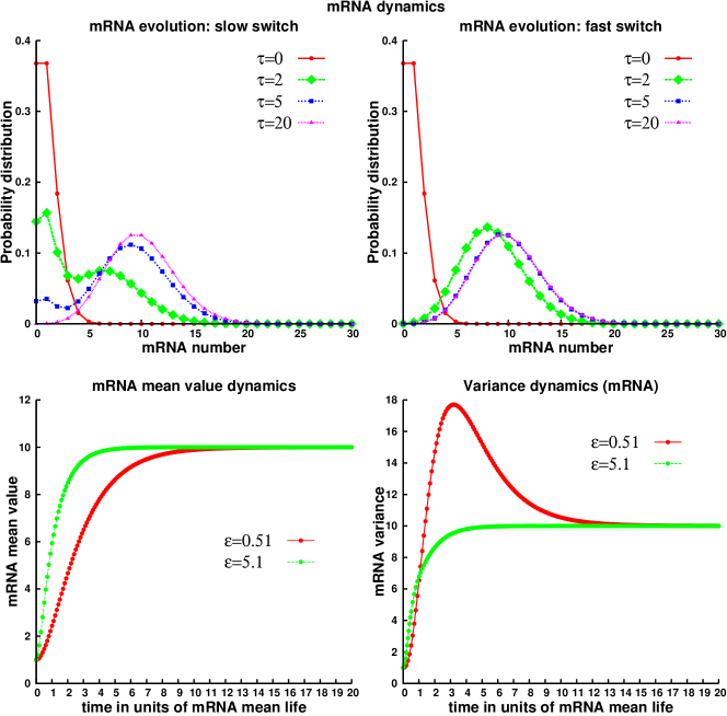
Figure 1: mRNA dynamics in slow ($\epsilon=0.51$) and fast ($\epsilon=5.1$) switch regimes. Remaining parameters: $N_{1}=10$, $N_{2}=1$, $p_{1}=1$, $p_{2}=0$.

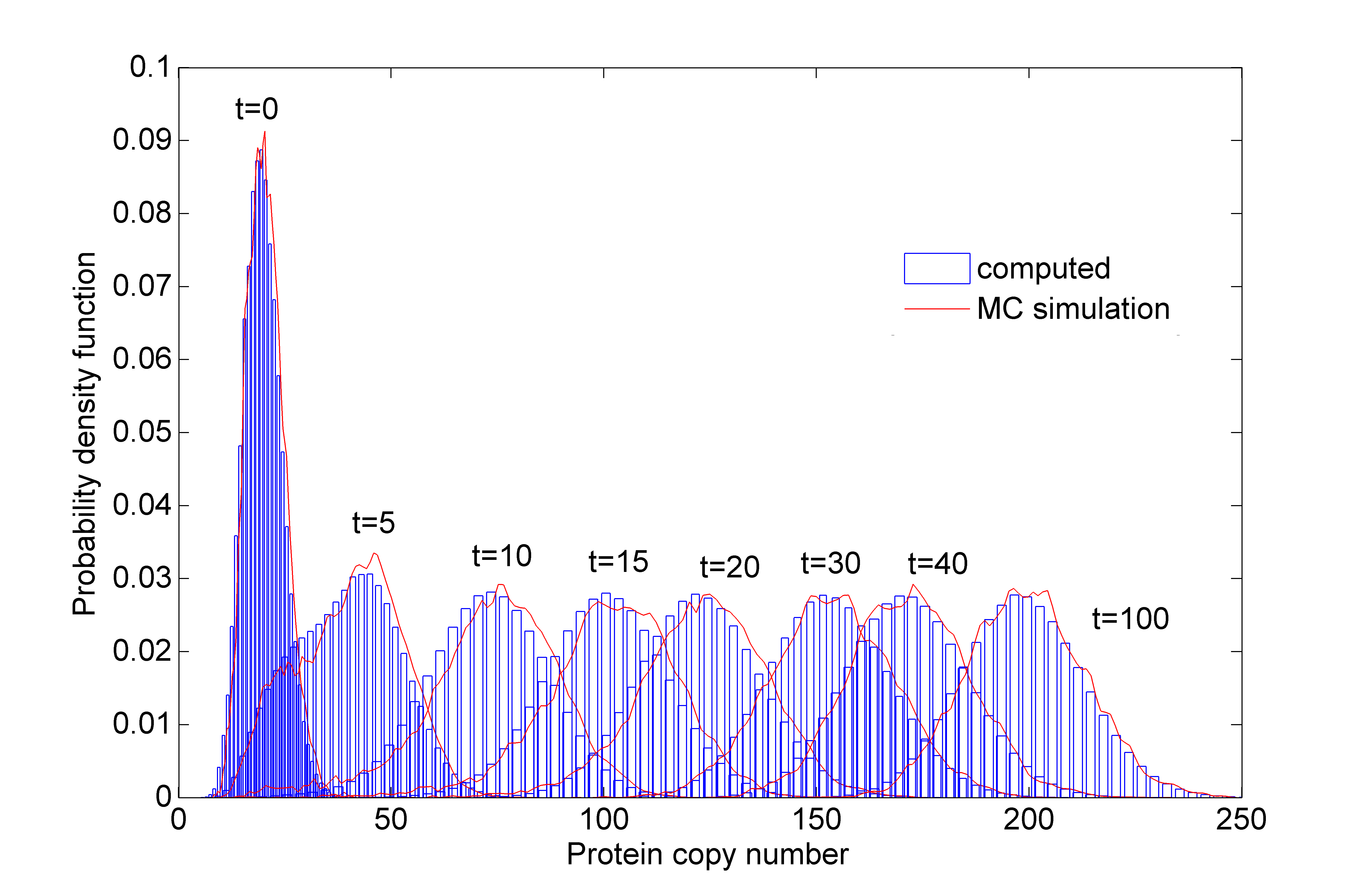
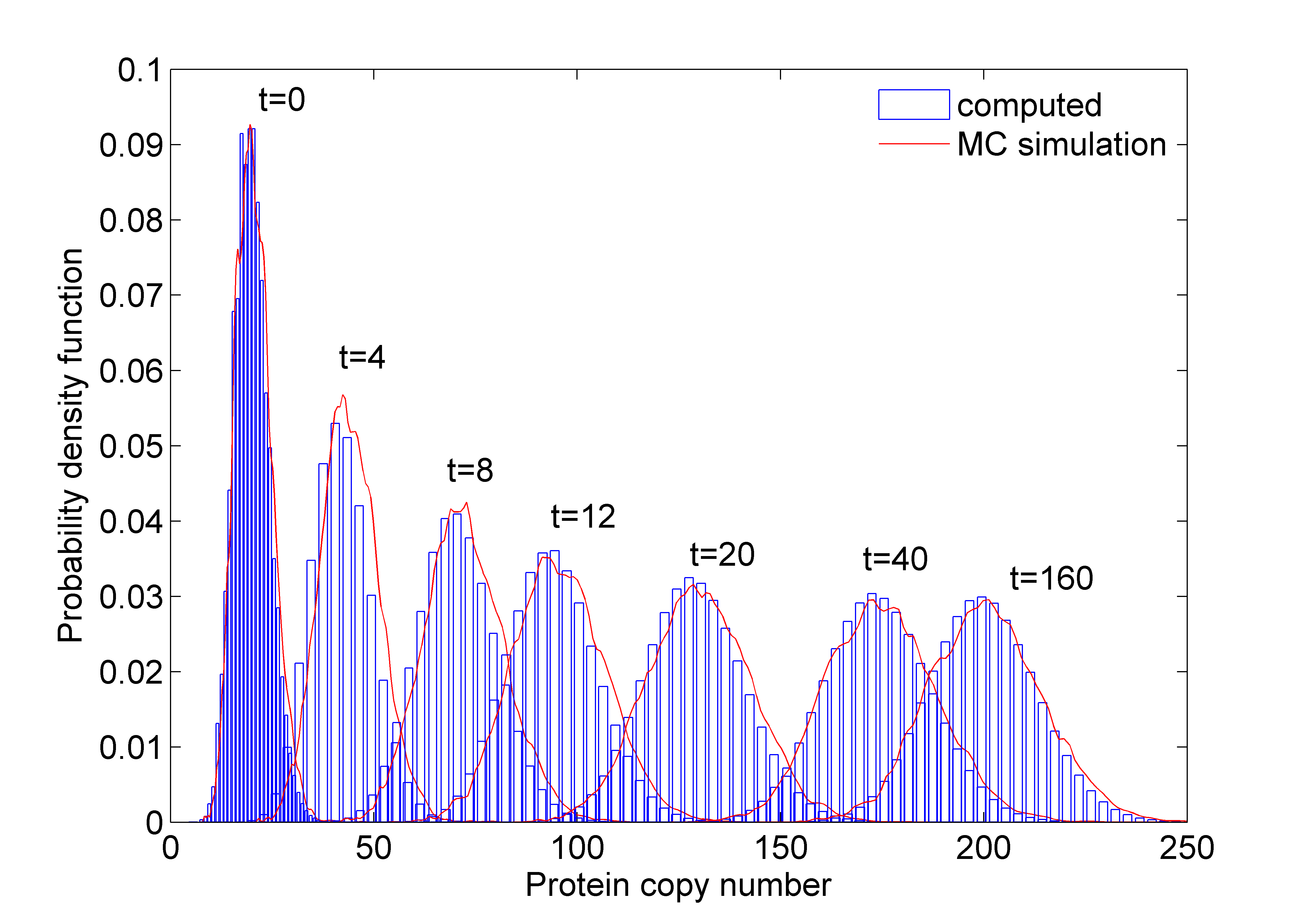
Figure 2: Comparison with Monte Carlo (MC) simulation. Slow switch ($\epsilon=0.51$) in Fig. 2 and fast switch ($\epsilon=5.1$) in Fig. 2. Remaining parameters: $N_{1}=10$, $N_{2}=1$, $p_{1}=1$, $p_{2}=0$, $\alpha=1/20$, $\beta=1$.

The result of this calculation is an ensemble of protein density values with their corresponding probabilities, $\{(m_{\tau}^{k},\mathbf{P}(m_{\tau}^{k})):k=1,\ldots,(L+1)^{p}\}$. Graphically, such ensembles will be represented by histograms where the probabilities are summed up within each bin. More precisely, if we fix a bin size and group together all $m_{\tau}^{k}$ belonging to the same bin, the probability assigned to that bin is simply the sum of all the probabilities $\mathbf{P}(m_{\tau}^{k})$ corresponding to the $m_{\tau}^{k}$ in that bin.

In order to estimate the accuracy of our method, we compare the distributions obtained by our formalism with those from a Monte Carlo (MC) simulation of the model. We have used the MC simulation to generate trajectories of the mRNA process $n_{\tau}$. Namely, let the $\tau_{q}$ be the random times when the birth and death process for mRNA molecules produces a change from $n_{\tau}$ to $n_{\tau}\pm 1$. Then Eq. (11) can be used to directly compute samples of the protein process $m_{\tau}$. Note that this makes our hybrid model much easier to simulate than the full discrete mRNA/protein model, since we avoid the separate simulation of the protein process, which is computationally costly.

As an example of our results we exhibit in Fig. 1 the time evolution for the probability distribution of the mRNA population, its mean value and variance. In all cases, we have used as initial mRNA configuration the generating function $\,\phi(\mu)=\exp(-N_{2}\mu)$, representing the gene with probability one in the off state, that is, the initial mRNA number follows a Poisson distribution with mean equal to $N_{2}$. On the other hand, the occupancy probabilities have been chosen as $p_{1}=1$, $p_{2}=0$, so as to produce a final equilibrium state which represents the gene in full activity and with mRNA number following a Poisson distribution with mean equal to $N_{1}$. Concerning the switching parameter $\epsilon$, we have selected two values: $\epsilon=5.1$ representing the “fast switch regime” and $\epsilon=0.51$ representing the “slow switch regime”. Specifically, in Fig. 2 we exhibit, for the two switch regimes, a direct comparison between the distributions obtained by our method (blue histograms) and those from MC simulation (red curves), and finally, in Fig. 3 we show the mean value and variance of the protein distribution, comparing the analytical formulas presented in Section 4 with the results of a direct simulation of the model.

Figure 3: Dynamical evolution of protein mean value and variance. Slow switch ($\epsilon=0.51$) in Fig. 3 and fast switch ($\epsilon=5.1$) in Fig. 3. Remaining parameters: $N_{1}=10$, $N_{2}=1$, $p_{1}=1$, $p_{2}=0$, $\alpha=1/20$, $\beta=1$.

The transient behavior of mRNA in the slow switch regime has a two peak distribution, indicating a more noisy configuration as compared to the fast switch regime, where the distribution is unimodal. The multi-modality in the slow switch regime is reflected in the protein probability density, where for time $\tau=5$, in Fig. 2, one can see the existence of a strong asymmetry. Also, it accounts for an increase in the noise of protein synthesis in the transient time, captured in the overshoot in Fig.3. Increasing the gene switch parameter decreases the standard deviation in mRNA production, which is a well known effect Innocentini2007 ; Innocentini2013 .

6 Discussion and Conclusion

The hybrid model presented here shows how to couple transcription and translation providing a complete picture of the entire dynamical process, without any restrictions on the parameter space. The randomness of protein synthesis due to the stochastic nature of transcription is exhibited in the dynamical behavior of the protein probability density. The main result is a full time-dependent solution for the probability distribution of mRNA as well as for the density probability for protein numbers – something that, to the best of our knowledge, has never been achieved before. Moroever, the distributions for protein number obtained by our method are in excellent agreement with those derived from MC simulations, at highly reduced computational cost. But there is a technical issue that must still be overcome. Namely, in order to improve the precision of our method, we must use joint probabilities with many events overlapping in a specific time interval (bigger values of $p$). The optimization in the implementation of our method necessary to deal with this issue will be left to future work.

It is worth mentioning that pure random differential equations (RDE) models – where the processes of mRNA production and of protein production are treated on equal footing, using random differential equations for both – have been introduced in LPCBK2006 for the continuous time case and in FBB2009 ; FBA2013 for the discrete time case. Similarly, pure master equations (ME) models – where the processes of mRNA production and of protein production are also treated on equal footing, but using master euations for both – have been discussed in the literature before; see, for instance Innocentini2007 ; Swain2008 . Both of these approaches are highly interesting and logically perfectly consistent, but a closer look reveals some drawbacks. On the one hand, using pure RDE models means that mRNA is represented by a continuous random variable, which is problematic since the number of mRNA molecules is small, of the order of a few dozen per gene. On the other hand, pure ME models are hard to solve explicitly and one has to resort to simulations or appeal to some approximation scheme in order to simplify the equations and then find expressions for the protein distribution (a discrete probability distribution) that solve these simplified equations, rather than the original ones.

Recent experiments allowing real-time observation of the expression of stochastic protein synthesis in living Escherichia coli or Bacillus subtilis cells, with single molecule sensitivity CFX2006 ; ovidiu1 , have shown that information about key parameters of protein expression can be extracted from the steady state distribution. Furthermore, measurements of protein concentration can be integrated with mRNA tagging techniques, such as MS2, that monitor mRNA production. The model discussed here can be used to extract quantitative information on transcription and translation processes from measured mRNA and protein distributions. In addition, the ability to compute the shape of the protein distribution may be used to improve the understanding of stochasticity in biological decision making processes.

Future research will also be dedicated to developing the model to include other phenomenological aspects of gene expression. One modification consists in allowing the protein synthesis/degradation rates to be random variables, thus taking into account the inherent noise due to the translational process. The model can also be extended to study eukaryotes, which requires introducing a time-delay accounting for the transport of mRNA from the nucleus to the cytoplasm. Another modification amounts to adding a non-linear term to the RDE, reflecting a decrease in protein number due to other effects than just degradation, such as complex formation by dimerization: this will introduce a bifurcation parameter and ultimately implement the observed multi-stability in the steady state of protein population (the bifurcation theory for RDEs can be found in Arnold1998 ). In contrast to multi-stability, the multi-modality originating in the controlling mechanism of protein synthesis, at the translational level, can be introduced by allowing the parameter $B$ (or $\beta$) in Eq. (2) to be a matrix, turning the RDE for protein density into a vector equation. The entries of this matrix will encode the different levels of translational efficiency.

Finally, the model can be used as a building block for constructing mathematical models of gene regulatory networks. More concretely, the idea is to take several copies of our model and couple them by allowing the binding/unbinding rates controlling the on/off switch of any gene to become functions of the mean values of the proteins expressed by the other genes. Traditionally, this coupling is performed through Hill type functions which convert protein densities into binding/unbinding rates. This strategy is in accordance with the ubiquitous idea in physics that simple models serve as building blocks for more complicated ones.

Acknowledgments.

We would like to thank the referees for their insights. Work supported by FAPESP, SP, Brazil (G.I., contract 2012/04723-4) and CNPq, Brazil (G.I., contract 202238/2014-8; M.F., contract 307238/2011-3; F.A., contract 306362/2012-0). O.R. thanks CNRS and LABEX Epigenmed for support.

References

- (1) Abramowitz, M., Stegun, I.A.: Handbook of mathematical functions with formulas, graphs and mathematical tables. U.S. Government Printing Office (1964)
- (2) Arnold, L.: Random dynamical systems. Springer-Verlag, Berlin (1998)
- (3) Blake, W.J., Kaern, M., Cantor, C.R., Collins, J.J.: Noise in eukaryotic gene expression. Nature 422, 633–637 (2003)
- (4) Cai, L., Friedman, N., Xie, X.: Stochastic protein expression in individual cells at the single molecule level. Nature 440(7082), 358–362 (2006). DOI 10.1038/nature04599
- (5) Cogburn, R., Torrez, W.C.: Birth and death processes with random environments in continuous time. J Appl Probab 18(1), 19–30 (1981)
- (6) Delbrück, M.: Statistical fluctuations in autocatalytic reactions. Journal of Chemical Physics 8, 120–124 (1940)
- (7) Elowitz, M.B., Levine, A.J., Siggia, E.D., Swain, P.S.: Stochastic gene expression in a single cell. Science 297(5584), 1183–1186 (2002). DOI 10.1126/science.1070919
- (8) Ferguson, M., Le Coq, D., Jules, M., Aymerich, S., Radulescu, O., Declerck, N., Royer, C.: Reconciling molecular regulatory mechanisms with noise patterns of bacterial metabolic promoters in induced and repressed states. P Natl Acad Sci USA 109(1), 155–160 (2012)
- (9) Ferreira, R.C., Bosco, F.A.R., Briones, M.R.S.: Scaling properties of transcription profiles in gene networks. Int J Bioinform Res Appl 5(2), 178–186 (2009)
- (10) Ferreira, R.C., Briones, M.R.S., Antoneli, F.: A model of gene expression based on random dynamical systems reveals modularity properties of gene regulatory networks. Preprint, arXiv:1309.0765
- (11) Friedman, N., Cai, L., Xie, X.S.: Linking stochastic dynamics to population distribution: an analytical framework of gene expression. Phys Rev Lett 97(16), 168302 (2006). DOI 10.1103/PhysRevLett.97.168302
- (12) Golding, I., Paulsson, J., Zawilski, S., Cox, E.: Real-time kinetics of gene activity in individual bacteria. Cell 123(6), 1025–1036 (2005). DOI 10.1016/j.cell.2005.09.031
- (13) Hornos, J.E.M., Schultz, D., Innocentini, G.C.P., Wang, J., Walczak, A.M., Onuchic, J.N., Wolynes, P.G.: Self-regulating gene: An exact solution. Phys Rev E 72(5), 051907 (2005). DOI 10.1103/PhysRevE.72.051907
- (14) Innocentini, G.C.P., Forger, M., Ramos, A., Radulescu, O., Hornos, J.E.M.: Multimodality and flexibility of stochasctic gene expression. Bull Math Biol 75, 2600–2630 (2013) DOI 10.1007/s11538-013-9909-3
- (15) Innocentini, G.C.P., Hornos, J.E.M.: Modeling stochastic gene expression under repression. Journal of Mathematical Biology 55(3), 413–431 (2007). DOI 10.1007/s00285-007-0090-x
- (16) Iyer-Biswas, S., Hayot, F., Jayaprakash, C.: Stochasticity of gene products from transcriptional pulsing. Phys Rev E 79(3), 031911 (2009). DOI 10.1103/PhysRevE.79.031911
- (17) van Kampen, N.G.: Stochastic Processes in Physics and Chemistry, 3rd edn. Elsevier, Amsterdam (2007)
- (18) Kepler, T.B., Elston, T.C.: Stochasticity in transcriptional regulation: origins, consequences, and mathematical representations. Biophys J 81(6), 3116–3136 (2001). DOI 10.1016/S0006-3495(01)75949-8
- (19) Lipniacki, T., Paszek, P., Marciniak-Czochra, A., Brasier, A.R., Kimmel, M.: Transcriptional stochasticity in gene expression. J Theor Biol 238, 348–367 (2006). DOI 10.1016/j.jtbi.2005.05.032
- (20) Ozbudak, E.M., Thattai, M., Kurtser, I., Grossman, A.D., van Oudenaarden, A.: Regulation of noise in the expression of a single gene. Nature Genetics 31, 69–73 (2002)
- (21) Paulsson, J.: Models of stochastic gene expression. Phys Life Rev 2, 157–175 (2005)
- (22) Peccoud, J., Ycart, B.: Markovian modeling of gene product synthesis. Theor Popul Biol 48(2), 222–234 (1995). DOI 10.1006/tpbi.1995.1027
- (23) Pirone, J., Elston, T.: Fluctuations in transcription factor binding can explain the graded and binary responses observed in inducible gene expression. J Theor Biol 226, 111–121 (2004). DOI 10.1016/j.jtbi.2003.08.008
- (24) Ramos, A.F., Innocentini, G.C.P., Hornos, J.E.M.: Exact time-dependent solutions for a self-regulating gene. Phys Rev E 83(6), 062902 (2011). DOI 10.1103/PhysRevE.83.062902
- (25) Raser, J.M., O’Shea, E.K.: Control of stochasticity in eukaryotic gene expression. Science 304(5678), 1811–1814 (2004). DOI 10.1126/science.1098641
- (26) Shahrezaei, V., Swain, P.S.: Analytical distributions for stochastic gene expression. P Natl Acad Sci USA 105(45), 17256–17261 (2008). DOI 10.1073/pnas.0803850105.
- (27) Yu, J., Xiao, J., Ren, X., Lao, K., Xie, X.S.: Probing gene expression in live cells, one protein molecule at a time. Science 311(5767), 1600–1603 (2006). DOI 10.1126/science.1119623