D2D Enhanced Heterogeneous Cellular Networks with Dynamic TDD

Abstract

Over the last decade, the growing amount of UL and DL mobile data traffic has been characterized by substantial asymmetry and time variations. Dynamic time-division duplex (TDD) has the capability to accommodate to the traffic asymmetry by adapting the UL/DL configuration to the current traffic demands. In this work, we study a two-tier heterogeneous cellular network (HCN) where the macro tier and small cell tier operate according to a dynamic TDD scheme on orthogonal frequency bands. To offload the network infrastructure, mobile users in proximity can engage in D2D communications, whose activity is determined by a carrier sensing multiple access (CSMA) scheme to protect the ongoing infrastructure-based and D2D transmissions. We present an analytical framework to evaluate the network performance in terms of load-aware coverage probability and network throughput. The proposed framework allows to quantify the effect on the coverage probability of the most important TDD system parameters, such as the UL/DL configuration, the base station density, and the bias factor. In addition, we evaluate how the bandwidth partition and the D2D network access scheme affect the total network throughput. Through the study of the tradeoff between coverage probability and D2D user activity, we provide guidelines for the optimal design of D2D network access.

I Introduction

As social applications in current data-centric networks continue to increase, mobile operators need to address the exponential growth of data traffic. Deploying diverse low-power small cell access points (SAPs) to complement the conventional macrocell network has proven as a cost-effective means to increase the network capacity and enhance coverage [1, 2, 3, 4]. Another technique to address the explosion of mobile data traffic is device-to-device (D2D) communications [5, 6]. With this technology, mobile users in proximity can establish a direct link and bypass the base stations, thereby offloading the network infrastructure and providing increased spectral efficiency [7, 8, 9, 10, 11, 12]. With tools from stochastic geometry [13], tractable analytical frameworks were developed for the design of D2D spectrum sharing in frequency-division duplex (FDD) cellular networks [7, 8, 9, 12]. Game theoretic models were applied to study the resource allocation for D2D communication in [6], [10], [11]. Specifically, Xu et al. [10] proposed a reverse iterative combinatorial auction based approach to efficiently assign the downlink (DL) cellular resource to D2D users. The uplink (UL) resource allocation issue between D2D and cellular users was investigated in [11], in which a coalition formation game model was proposed to maximize the system sum rate. Aside from the surge in data traffic, Internet services and video applications also lead to asymmetry and dynamic variations in the UL and DL traffic load. Time-division duplex (TDD) systems [14] have the capability to manage the UL/DL traffic asymmetry by adjusting the fraction of time dedicated to UL and DL transmissions, which we refer to as the UL/DL configuration, to the current traffic conditions. To accommodate the instantaneous traffic load among different cells, dynamic TDD with variable UL/DL configuration is under consideration and allows to make better use of the resources [15, 16].

In a two-tier HCN operating with universal frequency reuse, the major challenge is the cross-tier and co-tier interference. In addition, extra interference is imposed to the cellular transmissions if underlaid D2D transmissions are admitted. In a network operating with dynamic TDD, interference conditions can be severe and strong DL-to-UL (base station-to-base station) interference may lead to an unacceptable performance in the UL transmissions [17]. Considering the base stations and mobile users distribute as poisson point processes (PPPs), Yu et al. [18] derived the distributions of DL and UL SINR at an arbitrary mobile user and base station in a single tier dynamic TDD small cell network. However, the effect of important parameters such as UL/DL configuration and base station density on the network performance was not analyzed. Considering a two-tier HCN, a cognitive hybrid division duplex (CHDD) scheme was proposed in [19], where the macrocells operate with FDD, and small cells operate dynamic TDD on both FDD bands. Without interference management, [19] demonstrates that universal frequency reuse leads to a significant deterioration in the UL signal quality. To alleviate the cross-tier interference in a two-tier HCN, variable interference management schemes have been proposed, such as power control [20], interference cancellation [21], and spectrum allocation [22]. For spectrum allocation, a distributed disjoint subchannel allocation policy is sensible especially in dense small cell networks [22]. To address the co-tier interference, medium access control (MAC) is an effective and widely used technique in distributed ad hoc/sensor networks [23, 24, 25, 26]. Carrier sensing multiple access (CSMA) is a popular MAC protocol where the positions of simultaneously transmitting nodes can be modeled by a Matern Hard-core Process (MHP) [23, 24, 25]. In an MHP, each node respects a minimum exclusion distance with respect to each other so as to control the mutual interference. Carrier sensing is also employed in cognitive radio networks to limit the interference inflicted on primary users (PUs). In [26], secondary users (SUs) are modeled as a Poisson Hole Process (PHP), such that only SUs located outside the exclusion region of PUs can transmit.

Despite the fact that both the merit of dynamic TDD networks [15, 16], and the benefit of D2D communications in FDD networks [7, 8, 9] have been widely discussed in literature, a unifying framework for D2D enhanced TDD networks is still missing. In this work, we consider a D2D enhanced two-tier HCN operating with dynamic TDD where macrocells and small cells operate on two orthogonal frequency bands to eliminate the cross-tier interference. D2D users share the same bandwidth with the small cell tier and control their interference by means of a CSMA scheme. Furthermore, prior literature usually considers a fully-loaded model where every Voronoi cell has mobile users to connect. However, due to the small coverage of SAPs, the fully-loaded model may significantly overstate the network interference from small cells, leading to a pessimistic estimation on the coverage probability. In this work, we consider a load-aware model, where the empty cells are considered and the density of active cells is derived. Our main contributions can be listed as follows:

• We propose a simple PPP model for the active D2D transmitters based on the combined effect of a PHP and an MHP process, and we illustrate the validity of the PPP approximation by means of extensive simulations.

• We define an association policy that decouples the cell associations in UL and DL, and present an analytical framework that describes the load-aware coverage probability and network throughput as a function of all relevant system parameters. Although the effect of base station density and bias factor on the coverage probability is well understood in FDD networks [27], the effect of these system parameters in dynamic TDD networks is still unclear.

• We evaluate the effect of D2D network access scheme on network performance, and quantify its advantage over the random access scheme ALOHA.

• We study the tradeoff between coverage probability and D2D user activity. From the perspective of total network throughput, we provide guidelines for the optimal design of the network access scheme in D2D enhanced TDD networks.

The rest of the paper is organized as follows. In Section II, the system model is presented. In Section III, the load-aware coverage probability and network throughput are derived and the validity of the analytical framework is demonstrated by means of the numerical simulations. In Section IV, the impact of key parameters on the network coverage probability is evaluated and operating guidelines for the practical network design are provided. In Section V, the effect of bandwidth partition between the tiers and the impact of D2D network access control on the network performance are evaluated. Conclusions are given in Section VI.

II System Model

II-A Network Model

We consider a two-tier HCN which consists of a first tier of macro base stations (MBSs) distributed according to a homogeneous PPP $\Phi_{\mathtt{m}}$ with density $\lambda_{\mathtt{m}}$, overlaid with a network of SAPs distributed according to a PPP $\Phi_{\mathtt{s}}$ with density $\lambda_{\mathtt{s}}$. Mobile users are scattered over $\mathbb{R}^{2}$ according to a PPP $\Phi_{\mathtt{u}}$ with density $\lambda_{\mathtt{u}}$. A fraction $\zeta$ of the mobile users have their target receiver within a close distance and are considered as potential D2D transmitters. As an independent thinning of $\Phi_{\mathtt{u}}$ with probability $\zeta$, the set of potential D2D transmitters $\tilde{\Phi}_{\mathtt{d}}=\{T_{i}\}$ forms a PPP with density $\zeta\lambda_{\mathtt{u}}$. We assume that each potential D2D transmitter has an assigned receiver (not belonging to $\Phi_{\mathtt{u}}$) at a fixed distance $r_{\mathtt{d}}$ in a uniformly random direction. We consider orthogonal spectrum allocation where the total bandwidth $W$ is divided into two non-overlapping parts $\eta W$ and $\left(1-\eta\right)W$ that are allocated to the macro tier and small cell tier as depicted in Fig. 1. The potential D2D users share the spectrum with the small cell tier, thus leading to coexistence issues with the small cell users and SAPs. Both the macro tier and small cell tier operate according to the dynamic TDD scheme where at each timeslot a cell configures flexibly in DL or UL mode. The transmission mode selection for macrocells and small cells is modeled by independent Bernoulli random variables (r.v.’s), such that macrocells and small cells are configured in DL mode with probability $q_{\mathtt{D},\mathtt{m}}$ and $q_{\mathtt{D},\mathtt{s}}$, respectively, while the corresponding UL mode probabilities are given by $1-q_{\mathtt{D},\mathtt{m}}$ and $1-q_{\mathtt{D},\mathtt{s}}$. The multiplexing probabilities $q_{\mathtt{D},\mathtt{m}}$ and $q_{\mathtt{D},\mathtt{s}}$ define the UL/DL configuration for the macro tier and small cell tier. The concurrent DL and UL transmissions in neighboring cells may lead to new types of inter-cell interference, i.e. DL-to-UL and UL-to-DL (user-to-user) interference. Let $P_{\mathtt{m}}$, $P_{\mathtt{s}}$, $Q_{\mathtt{m}}$ and $Q_{\mathtt{s}}$ denote the transmit power of MBSs, SAPs, mobile users associated with the macro tier, and mobile users associated with the small cell tier. We use $Q_{\mathtt{d}}$ to represent the transmit power of potential D2D users. To avoid confusion, in the following parts the term mobile users only denotes the mobile users that are expected to communicate via infrastructures, while the term potential D2D users refers to mobile users which attempt to communicate with each other by employing D2D technology.

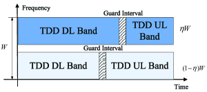
Figure 1: Dynamic TDD scheme in two-tier heterogeneous cellular networks.

We consider a load-aware resource allocation model where each base station always has data to transmit if it has a mobile user within its coverage. We adopt orthogonal multiple access, such that within a cell only a single mobile user can be active at any given timeslot and subchannel. If several mobile users connect to the same base station, the base station will randomly choose one mobile user to serve. To control the interference inflicted by D2D transmissions on small cell transmissions, we provide medium access control by means of a CSMA scheme. The channel model consists of path loss and flat-fading. The fading power from a transmitter located at point $x$ to the typical receiver located at the origin is denoted by $h_{ox}$ and is assumed to be an independent and identically distributed (i.i.d.) exponential r.v., $h\sim\textrm{exp(1)}$, which corresponds to Rayleigh fading. The path loss function is given by $g\left(\|x\|\right)=\|x\|^{-\alpha}$, with $\alpha>2$ the path loss exponent. Due to the slight impact of thermal noise in current heterogeneous networks, we consider the interference-limited regime, and ignore the thermal noise [29].

II-B Cell Association

At each timeslot, a mobile user acts as a transmitter or receiver with probability $\mu$ and $1-\mu$, respectively. Assuming open access, the association of a mobile user to a given tier is based on the maximum biased received signal power averaged over fading. The bias factor in this association policy is used to balance the traffic load among different tiers. In this paper, we consider a decoupled DL and UL association model as follows.

II-B1 Downlink Association Policy

A typical receiver is associated with the nearest base station in DL mode of tier $i$ if

$$i=\arg\underset{k\in\{\mathtt{m},\,\mathtt{s}\}}{\max}P_{k}B_{\mathtt{D},k}D_{\mathtt{D},k}^{-\alpha},$$ (1)

where $B_{\mathtt{D},k}$ is the DL bias factor of tier $k$, and $D_{\mathtt{D},k}$ denotes the distance from the typical receiver to the nearest base station of $\Phi_{k}$ operating in DL mode with thinned density $q_{\mathtt{D},k}\lambda_{k}$.

II-B2 Uplink Association Policy

A typical transmitter is associated with the nearest base station in UL mode of tier $i$ if

$$i=\arg\underset{k\in\{\mathtt{m},\,\mathtt{s}\}}{\max}Q_{k}B_{\mathtt{U},k}D_{\mathtt{U},k}^{-\alpha},$$ (2)

where $B_{\mathtt{U},k}$ is the UL bias factor of tier $k$, $D_{\mathtt{U},k}$ denotes the distance from the typical transmitter to the nearest base station of $\Phi_{k}$ operating in UL mode with thinned density $\left(1-q_{\mathtt{D},k}\right)\lambda_{k}$.

For notational brevity, we define the normalized parameters of tier $k$ conditioned on the serving tier $i$.

$$\hat{\lambda}_{k}^{(i)}\triangleq\frac{\lambda_{k}}{\lambda_{i}},\>\hat{q}_{\mathtt{D},k}^{(i)}\triangleq\frac{q_{\mathtt{D},k}}{q_{\mathtt{D},i}},\>\hat{q}_{\mathtt{U},k}^{(i)}\triangleq\frac{1-q_{\mathtt{D},k}}{1-q_{\mathtt{D},i}},\>$$

$$\hat{P}_{k}^{(i)}\triangleq\frac{P_{k}}{P_{i}},\>\hat{Q}_{k}^{(i)}\triangleq\frac{Q_{k}}{Q_{i}},\>\hat{B}_{\mathtt{D},k}^{(i)}\triangleq\frac{B_{\mathtt{D},k}}{B_{\mathtt{D},i}},\>\hat{B}_{\mathtt{U},k}^{(i)}\triangleq\frac{B_{\mathtt{U},k}}{B_{\mathtt{U},i}}.$$ (3)

Using the association rules defined in (1) and (2), the set of base stations form different multiplicatively weighted Voronoi tessellations of the two dimensional plane in DL and UL.

Definition 1.

The downlink and uplink association regions of an MBS or a SAP located at point $x$ are given by (4) and (5), respectively [30]

$$\mathcal{C}_{\mathtt{D},x} = \Bigl{\{}y\in\mathbb{R}^{2}|\|y-x\|\leq\bigl{(}\hat{P}_{k}^{(i)}\hat{B}_{\mathtt{D},k}^{(i)}\bigr{)}^{-\frac{1}{\alpha}}$$ (4)

$$\times\|y-X_{\mathtt{D},k}^{*}\left(y\right)\|,\forall k\in\{\mathtt{m},\,\mathtt{s}\}\Bigr{\}},$$

$$\mathcal{C}_{\mathtt{U},x} = \Bigl{\{}y\in\mathbb{R}^{2}|\|y-x\|\leq\Bigl{(}\hat{Q}_{k}^{(i)}\hat{B}_{\mathtt{U},k}^{(i)}\Bigr{)}{}^{-\frac{1}{\alpha}}$$ (5)

$$\times\|y-X_{\mathtt{U},k}^{*}\left(y\right)\|,\forall k\in\{\mathtt{m},\,\mathtt{s}\}\Bigr{\}},$$

where $X_{\mathtt{D},k}^{*}\left(y\right)$ and $X_{\mathtt{U},k}^{*}\left(y\right)$ denote the corresponding distances from $y$ to the nearest DL base station and to the UL base station of tier k.

As a consequence, a mobile user may associate with different base stations for DL and UL traffic. Let $\mathcal{N}_{\mathtt{D},i}$ and $\mathcal{N}_{\mathtt{U},i}$ denote the DL load and UL load, defined as the number of mobile users served by a base station of tier $i$ operating in DL and UL.

II-C CSMA model of potential D2D users

At the start of a timeslot, each potential D2D transmitter senses the active small cell transmissions which originate from SAPs in DL mode and transmitting mobile users associated with the small cell tier. Assuming channel reciprocity, the potential D2D transmitter predicts the would-be interference it may impose on the small cell transmitters and refrains from transmitting if the interference exceeds the protection threshold $\rho_{\mathtt{s}}$. As such, D2D transmissions respect an exclusion region around each small cell transmitter. The remaining potential D2D transmitters form a PHP, which can be approximated by a PPP [26]. Carrier sensing is also performed with respect to the remaining potential D2D transmitters, where the signal power from a nearby D2D transmitter is not allowed to surpass the contention threshold $\rho_{\mathtt{d}}$. To resolve the collision among the D2D contenders, we use a back-off scheme. Specifically, each remaining D2D transmitter independently samples a random timer $t_{i}\sim\mathcal{U}[0,1]$ and channel access is granted to the contender with the smallest timer within a contention region [23].

Let $U_{i}$ be the retention indicator of the $i$-th potential D2D transmitter $T_{i}$, which is given by

$$U_{i} = \prod_{Y_{j}\in\Phi_{\mathtt{s}}^{\mathtt{D}}}\mathbf{1}_{\bigl{(}\frac{Q_{\mathtt{d}}h_{ji}}{\|T_{i}-Y_{j}\|^{\alpha}}<\rho_{\mathtt{s}}\bigr{)}}\prod_{Z_{l}\in\Phi_{\mathtt{u},\mathtt{s}}^{\mathtt{T}}}\mathbf{1}_{\bigl{(}\frac{Q_{\mathtt{d}}h_{li}}{\|T_{i}-Z_{l}\|^{\alpha}}<\rho_{\mathtt{s}}\bigr{)}}$$ (6)

$$\times \prod_{T_{k}\in\Phi_{\mathtt{d}}\backslash T_{i}}\Bigl{(}\mathbf{1}_{\left(t_{i}\leq t_{k}\right)}+\mathbf{1}_{\left(t_{i}>t_{k}\right)}\mathbf{1}_{\bigl{(}\frac{Q_{\mathtt{d}}h_{ki}}{\|T_{i}-T_{k}\|^{\alpha}}<\rho_{\mathtt{d}}\bigr{)}}\Bigr{)}$$

where $h_{ji}$ denotes the channel fading from $T_{i}$ to $Y_{j}$, $\{Y_{j}\}=\Phi_{\mathtt{s}}^{\mathtt{D}}$ denotes the set of active SAPs in DL, and $\{Z_{l}\}=\Phi_{\mathtt{u},\mathtt{s}}^{\mathtt{T}}$ represents the set of transmitting mobile users associated with the small cell tier. The first two products in (6) reflect that the interference inflicted by a potential D2D transmitter on an active small cell transmitter should be smaller than $\rho_{\mathtt{s}}$. The first term inside the last product corresponds to the event where the timer $t_{i}$ is smaller than $t_{k}$, while the second term corresponds to the event where the timer $t_{i}$ is larger than $t_{k}$, yet the interference from $T_{i}$ to $T_{k}$ is smaller than $\rho_{\mathtt{d}}$.

Define $\beta\overset{\triangle}{=}\Pr[U_{i}=1]$ as the retaining probability of $T_{i}$, which depends on the timer $t_{i}$, the channel fading and the distance between $T_{i}$ and small cell transmitters. The set of winning contenders forms a point process similar to the MHP, where any two points respect a minimum exclusion distance determined by $\rho_{\mathtt{d}}$ and the instantaneous channel gain. It is known that the aggregate interference experienced by a user of an MHP can be approximated by the interference resulting from a PPP that has the same density as the MHP and exists outside the exclusion region [24], [25]. In this work, we assume that each potential D2D transmitter is retained independently with the probability $\beta$. As a result, the retained D2D transmitters $\Phi_{\mathtt{d}}$ form a PPP with density $\beta\zeta\lambda_{\mathtt{u}}$, where the combined effect of PHP and MHP is captured by $\beta$. Note that the retained D2D transmitters are the actually active D2D transmitters in the current timeslot. The potential D2D transmitters that fail to access channel will keep silent in the current timeslot and continue to execute the CSMA scheme in the next timeslot.

III Performance Analysis

In this section, we derive the load-aware coverage probability and network throughput, and we validate the theoretical model by means of simulations.

III-A Association and Load Characterization

The probability that a typical receiving and transmitting mobile user is associated with tier $i$ for DL and UL, is given by

$$\mathcal{A}_{\mathtt{D},i} = \frac{q_{\mathtt{D},i}\lambda_{i}}{\sum_{k\in\{\mathtt{m},\mathtt{s}\}}G_{\mathtt{D},k}^{(i)}},\>\mathcal{A}_{\mathtt{U},i}=\frac{\left(1-q_{\mathtt{D},i}\right)\lambda_{i}}{\sum_{k\in\{\mathtt{m},\mathtt{s}\}}G_{\mathtt{U},k}^{(i)}},$$ (7)

where $G_{\mathtt{D},k}^{(i)}=q_{\mathtt{D},k}\lambda_{k}\left(\hat{P}_{k}^{(i)}\hat{B}_{\mathtt{D},k}^{(i)}\right)^{\frac{2}{\alpha}},\>G_{\mathtt{U},k}^{(i)}=\left(1-q_{\mathtt{D},k}\right)\lambda_{k}\left(\hat{Q}_{k}^{(i)}\hat{B}_{\mathtt{U},k}^{(i)}\right)^{\frac{2}{\alpha}}.$ The result is a corollary of Lemma 1 in [27] and extends the DL association policy to the dynamic TDD scheme. For the special case of $\{q_{\mathtt{D,m}},q_{\mathtt{D,s}}\}=\{0,0\}$, we define $\{\mathcal{A}_{\mathtt{D},\mathtt{m}},\mathcal{A}_{\mathtt{D},\mathtt{s}}\}=\{0,0\}$, and the network changes into a two-tier UL network. For $\{q_{\mathtt{D,m}},q_{\mathtt{D,s}}\}=\{1,1\}$, we define $\{\mathcal{A}_{\mathtt{U},\mathtt{m}},\mathcal{A}_{\mathtt{U},\mathtt{s}}\}=\{0,0\}$, and the network transforms to a two-tier DL network. The association probabilities defined in (7) indicate how the per tier association probability in a two-tier dynamic TDD network depends on the relative transmit power, bias factor, and base station density of the corresponding transmission mode. Note that the base station density affects the per tier association probability more than transmit power or bias factor.

By considering the traffic load, we derive a more accurate load-aware coverage probability. For each tier i, we compute the void probability of a random base station in DL and UL, i.e. $\mathbb{P}_{\mathit{\mathit{e}}}^{\mathtt{D},i}$ and $\mathbb{P}_{\mathit{\mathit{e}}}^{\mathtt{U},i}$, and compare it with a threshold value to determine the network traffic load. When $\mathbb{P}_{\mathit{\mathit{e}}}^{\mathtt{D},i}<10^{-4}$ and $\mathbb{P}_{\mathit{\mathit{e}}}^{\mathtt{U},i}<10^{-4}$, we say tier i is fully-loaded, otherwise, partially-loaded. Denote $\Phi_{\mathtt{m}}^{\mathtt{D}}\sim\textrm{PPP}(\lambda_{\mathtt{m}}^{\mathtt{D}})$, $\Phi_{\mathtt{s}}^{\mathtt{D}}\sim\textrm{PPP}(\lambda_{\mathtt{s}}^{\mathtt{D}})$, $\Phi_{\mathtt{m}}^{\mathtt{U}}\sim\textrm{PPP}(\lambda_{\mathtt{m}}^{\mathtt{U}})$ and $\Phi_{\mathtt{s}}^{\mathtt{U}}\sim\textrm{PPP}(\lambda_{\mathtt{s}}^{\mathtt{U}})$ as the point processes of active DL MBSs, DL SAPs, UL MBSs, and UL SAPs, respectively, with corresponding denstities $\lambda_{\mathtt{m}}^{\mathtt{D}}$, $\lambda_{\mathtt{s}}^{\mathtt{D}}$, $\lambda_{\mathtt{m}}^{\mathtt{U}}$ and $\lambda_{\mathtt{s}}^{\mathtt{U}}$. In the following lemma, we derive the void probability of a base station in tier i, and we determine the exact density of active base stations in DL and UL.

Lemma 1.

The probability that a cell of tier $i$ is void for DL and UL is derived as

$$\mathbb{P}_{\mathit{\mathit{e}}}^{\mathtt{D},i}=\Bigl{(}1+\frac{\bigl{(}1-\mu\bigr{)}\bigl{(}1-\zeta\bigr{)}\lambda_{\mathtt{u}}\mathcal{A}_{\mathtt{D},i}}{3.5q_{\mathtt{D},i}\lambda_{i}}\Bigr{)}^{-3.5},$$ (8)

$$\mathbb{P}_{\mathit{e}}^{\mathtt{U},i}=\Bigl{(}1+\frac{\mu\bigl{(}1-\zeta\bigr{)}\lambda_{\mathtt{u}}\mathcal{A}_{\mathtt{U},i}}{3.5\left(1-q_{\mathtt{D},i}\right)\lambda_{i}}\Bigr{)}^{-3.5}.$$ (9)

Furthermore, the density of active base stations in DL and UL mode of tier $i$ is given by

$$\lambda_{i}^{\mathtt{D}}=\lambda_{i}q_{\mathtt{D},i}\bigl{(}1-\mathbb{P}_{e}^{\mathtt{D},i}\bigr{)}\>\textrm{and}\>\lambda_{i}^{\mathtt{U}}=\lambda_{i}\bigl{(}1-q_{\mathtt{D},i}\bigr{)}\bigl{(}1-\mathbb{P}_{e}^{\mathtt{U},i}\bigr{)}.$$ (10)

Proof:

The results can be proved by a minor modification of Lemma 1 in [31]. Here we give the proof for completeness. The probability density function (PDF) of the area of a random Voronoi cell is given by $f_{X}(x)=\frac{3.5^{3.5}}{\Gamma(3.5)}x^{2.5}e^{-3.5x}$, where $X$ denotes the area of a random Voronoi cell normalized by the value $1/q_{\mathtt{D},i}\lambda_{i}$ in DL and $1/(1-q_{\mathtt{D},i})\lambda_{i}$ in UL mode. Taking the DL mode as an example, the PDF of the DL load $\mathcal{N}_{\mathtt{D},i}$ is given by

$$\mathbb{\Pr}[\mathcal{N}_{\mathtt{D},i}=n]$$

$$= \int_{0}^{\infty}\Pr[\mathcal{N}_{\mathtt{D},i}=n|X=x]\cdot f_{X}(x)dx$$

$$\overset{(a)}{=} \int_{0}^{\infty}\frac{1}{n!}\bigl{(}\frac{\lambda_{\mathtt{u},i}^{\mathtt{R}}x}{q_{\mathtt{D},i}\lambda_{i}}\bigr{)}^{n}e^{-\frac{\lambda_{\mathtt{u},i}^{\mathtt{R}}x}{q_{\mathtt{D},i}\lambda_{i}}}\cdot f_{X}(x)dx$$

$$\overset{(b)}{=} \frac{3.5^{3.5}}{n!}\frac{\Gamma\left(n+3.5\right)}{\Gamma\left(3.5\right)}\bigl{(}\frac{\lambda_{\mathtt{u},i}^{\mathtt{R}}}{q_{\mathtt{D},i}\lambda_{i}}\bigr{)}^{n}\bigl{(}3.5+\frac{\lambda_{\mathtt{u},i}^{\mathtt{R}}}{q_{\mathtt{D},i}\lambda_{i}}\bigr{)}^{-\left(n+3.5\right)}$$

where $\lambda_{\mathtt{u},i}^{\mathtt{R}}=\bigl{(}1-\mu\bigr{)}\bigl{(}1-\zeta\bigr{)}\lambda_{\mathtt{u}}\mathcal{A}_{\mathtt{D},i}$ denotes the density of the receiving mobile users associated with tier $i$, $q_{\mathtt{D},i}\lambda_{i}$ is the density of total DL base stations of tier $i$, $\Gamma(\cdot)$ is the gamma function, which is given by $\Gamma\left(x\right)=\int_{0}^{\infty}t^{x-1}\exp\left(-t\right)dt$, (a) is due to the definition of Poisson distribution, and (b) takes the expectation with respect to the area distribution $f_{X}(x)$. Substituting $n=0$ into (LABEL:eq:Load_exact) derives the void probability $\mathbb{P}_{e}^{\mathtt{D},i}=\Pr[\mathcal{N}_{\mathtt{D},i}=0]=\bigl{(}1+\frac{\lambda_{\mathtt{u},i}^{\mathtt{R}}}{3.5q_{\mathtt{D},i}\lambda_{i}}\bigr{)}^{-3.5}$, which concludes the proof. ∎

III-B Coverage Probability

With the PPP approximation and the void probability derived in (8), (9), we derive the load-aware coverage probability of tier $i$, $i\in\{\mathtt{m},\>\mathtt{s}\}$ in DL and UL as

$$\mathbb{P}_{i}^{\mathtt{D}}=\Pr[\mathtt{SIR}_{i}^{\mathtt{D}}>\gamma_{i}^{\mathtt{D}}],\;\mathbb{P}_{i}^{\mathtt{U}}=\Pr[\mathtt{SIR}_{i}^{\mathtt{U}}>\gamma_{i}^{\mathtt{U}}],$$ (12)

where $\gamma_{i}^{\mathtt{D}}$ and $\gamma_{i}^{\mathtt{U}}$ denote the SIR thresholds of DL and UL transmissions in tier $i$. Similarly, the coverage probability of a typical D2D receiver is $\mathbb{P}_{\mathtt{d}}=\Pr[\mathtt{SIR}_{\mathtt{d}}>\gamma_{\mathtt{d}}]$ with $\gamma_{\mathtt{d}}$ the SIR threshold of D2D user.

Since we consider open access, the distance between a typical mobile user and its serving base station of tier $i$ in DL or UL mode, $Y_{\mathtt{D},i}$ or $Y_{\mathtt{U},i}$, is not only influenced by $\Phi_{i}^{\mathtt{D}}$ or $\Phi_{i}^{\mathtt{U}}$, but also by $\Phi_{k}^{\mathtt{D}}$ or $\Phi_{k}^{\mathtt{U}}$, $k\neq i$. The distance distribution is given by

$$f_{Y_{\mathtt{D},i}}(y)=2\pi\frac{q_{\mathtt{D},i}\lambda_{i}}{\mathcal{A}_{\mathtt{D},i}}y\exp\{-\pi\frac{q_{\mathtt{D},i}\lambda_{i}}{\mathcal{A}_{\mathtt{D},i}}y^{2}\},$$ (13)

$$f_{Y_{\mathtt{U},i}}(y)=2\pi\frac{\left(1-q_{\mathtt{D},i}\right)\lambda_{i}}{\mathcal{A}_{\mathtt{U},i}}y\exp\{-\pi\frac{\left(1-q_{\mathtt{D},i}\right)\lambda_{i}}{\mathcal{A}_{\mathtt{U},i}}y^{2}\},$$ (14)

where the result is a modification of Lemma 4 in [27] for dynamic TDD networks.

The DL and UL SIR of a typical receiver associated with the macro tier is given by

$$\mathtt{SIR}_{\mathtt{m}}^{\mathtt{D}}=\frac{P_{\mathtt{m}}h_{or}r^{-\alpha}}{I_{\mathtt{D\rightarrow D}}^{\mathtt{(m)}}+I_{\mathtt{U\rightarrow D}}^{\mathtt{(m)}}},\;\mathtt{SIR_{m}^{U}}=\frac{Q_{\mathtt{m}}h_{or}r^{-\alpha}}{I_{\mathtt{D\rightarrow U}}^{\mathtt{(m)}}+I_{\mathtt{U\rightarrow U}}^{(\mathtt{m})}},$$ (15)

where $h_{or}$ and $r$ are the fading power and the typical link length, and

$$I_{\mathtt{D\rightarrow D}}^{\mathtt{(m)}}=\sum_{y\in\Phi_{\mathtt{m}}^{\mathtt{D}}\backslash\{y_{0}\}}P_{\mathtt{m}}h_{oy}y^{-\alpha},\>I_{\mathtt{U\rightarrow D}}^{\mathtt{(m)}}=\sum_{x\in\Phi_{\mathtt{u,m}}^{\mathtt{T}}}Q_{\mathtt{m}}h_{ox}x^{-\alpha},$$

$$I_{\mathtt{D\rightarrow U}}^{\mathtt{(m)}}=\sum_{y\in\Phi_{\mathtt{m}}^{\mathtt{D}}}P_{\mathtt{m}}h_{oy}y^{-\alpha},\>I_{\mathtt{U\rightarrow U}}^{(\mathtt{m})}=\sum_{x\in\Phi_{\mathtt{u,m}}^{\mathtt{T}}\backslash\{x_{0}\}}Q_{\mathtt{m}}h_{ox}x^{-\alpha},$$

where $y_{0}$ and $x_{0}$ represent the position of typical transmitter in DL and UL mode, $\Phi_{\mathtt{u},\mathtt{m}}^{\mathtt{T}}$ represents the set of transmitting mobile users associated with macro tier. Due to the orthogonal multiple access technology, there is a one-to-one mapping from the transmitting mobile users associated with macro tier to the active UL MBSs. Since the coupling between the location of MBSs and transmitting mobile users has little effect on the coverage probability [19, 28], we neglect the coupling and model $\Phi_{\mathtt{u},\mathtt{m}}^{\mathtt{T}}$ as a PPP with density $\lambda_{\mathtt{u,m}}^{\mathtt{T}}=\lambda_{\mathtt{m}}^{\mathtt{U}}$. The simulation results in Section IV also validate the accuracy of the approximation.

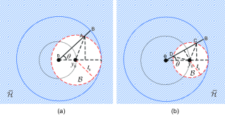
Figure 2: In the small cell tier, the typical receiver locates at the origin, and the serving transmitter $y_{0}$ employs $\iota_{\mathtt{s}}$ to form an exclusion region, within which no D2D transmitter can exist. (a) is for $\|y_{0}\|\leq\iota_{\mathtt{s}}$ and (b) is for $\|y_{0}\|>\iota_{\mathtt{s}}$.

The DL and UL SIR of a typical receiver associated with small cell tier is denoted by

$$\mathtt{SIR}_{\mathtt{s}}^{\mathtt{D}}=\frac{P_{\mathtt{s}}h_{or}r^{-\alpha}}{I_{\mathtt{D\rightarrow D}}^{\mathtt{(s)}}+I_{\mathtt{U\rightarrow D}}^{\mathtt{(s)}}+I_{\mathtt{d\rightarrow D}}},\>\mathtt{SIR}_{\mathtt{s}}^{\mathtt{U}}=\frac{Q_{\mathtt{s}}h_{or}r^{-\alpha}}{I_{\mathtt{D\rightarrow U}}^{\mathtt{(s)}}+I_{\mathtt{U\rightarrow U}}^{\mathtt{(s)}}+I_{\mathtt{d\rightarrow U}}},$$

(16)

where

$$I_{\mathtt{D\rightarrow D}}^{\mathtt{(s)}}=\sum_{y\in\Phi_{\mathtt{s}}^{\mathtt{D}}\backslash\{y_{0}\}}P_{\mathtt{s}}h_{oy}y^{-\alpha},\>I_{\mathtt{U\rightarrow D}}^{\mathtt{(s)}}=\sum_{x\in\Phi_{\mathtt{u},\mathtt{s}}^{\mathtt{T}}}Q_{\mathtt{s}}h_{ox}x^{-\alpha},$$

$$I_{\mathtt{d\rightarrow D}}=\sum_{z\in\Phi_{\mathtt{d}}\backslash b\left(y_{0},\iota_{\mathtt{s}}\right)}Q_{\mathtt{d}}h_{oz}z^{-\alpha},\>I_{\mathtt{D\rightarrow U}}^{\mathtt{(s)}}=\sum_{y\in\Phi_{\mathtt{s}}^{\mathtt{D}}}P_{\mathtt{s}}h_{oy}y^{-\alpha},$$

$$I_{\mathtt{U\rightarrow U}}^{\mathtt{(s)}}=\sum_{x\in\Phi_{\mathtt{u},\mathtt{s}}^{\mathtt{T}}\backslash\{x_{0}\}}Q_{\mathtt{s}}h_{ox}x^{-\alpha},\>I_{\mathtt{d\rightarrow U}}=\sum_{z\in\Phi_{\mathtt{d}}\backslash b\left(x_{0},\iota_{\mathtt{s}}\right)}Q_{\mathtt{d}}h_{oz}z^{-\alpha},$$

where $\Phi_{\mathtt{u},\mathtt{s}}^{\mathtt{T}}\sim\textrm{PPP}(\lambda_{\mathtt{u,s}}^{\mathtt{T}})$ represents the set of transmitting mobile users associated with small cell tier with density $\lambda_{\mathtt{u,s}}^{\mathtt{T}}=\lambda_{\mathtt{s}}^{\mathtt{U}}$. As is shown in Fig. 2, the active D2D transmitters are distributed in the shaded region, i.e. the whole $\mathbb{R}^{2}$ plane except for the exclusion region centered at $y_{0}$, which is approximated by a ball $\mathcal{B}$. The shaded region can be divided into two disjoint parts by the circle $\mathcal{H}$ with the center at the origin. Define $\mathcal{H}\overset{\triangle}{=}b\left(0,\|y_{0}\|+\iota_{\mathtt{s}}\right)$, $\mathcal{B}\overset{\triangle}{=}b\left(y_{0},\iota_{\mathtt{s}}\right)$, where $\mathcal{B}$ is the exclusion region for D2D transmissions around each small cell transmitter. Note that as a function of $\rho_{\mathtt{s}}$ and the instantaneous channel fading, the exclusion region is not a ball but an irregular shape, which varies in different timeslot. To simplify the analysis, we use a ball to approximate the exclusion region, where the equivalent exclusion distance is determined by imposing a small miss detection probability threshold $\epsilon$. The constraint is met when $\mathbb{\Pr}[Q_{\mathtt{d}}h_{x_{0}z}/\iota_{\mathtt{s}}^{\alpha}>\rho_{\mathtt{s}}]=\epsilon$, and solving for $\iota_{\mathtt{s}}$ yields $\iota_{\mathtt{s}}=\bigl{(}\frac{-\ln\epsilon}{\rho_{\mathtt{s}}/Q_{\mathtt{d}}}\bigr{)}^{\frac{1}{\alpha}}$, where $h_{x_{0}z}$ denotes the fading power from a D2D transmitter $z$ to the typical small cell transmitter $x_{0}$.

The SIR of a typical D2D receiver is given by

$$\mathtt{SIR_{d}}=\frac{Q_{\mathtt{d}}h_{or}r_{\mathtt{d}}^{-\alpha}}{I_{\mathtt{D\rightarrow d}}^{\mathtt{(s)}}+I_{\mathtt{U\rightarrow d}}^{\mathtt{(s)}}+I_{\mathtt{d\rightarrow d}}},$$ (17)

where

$$I_{\mathtt{D\rightarrow d}}^{\mathtt{(s)}}=\sum_{y\in\Phi_{\mathtt{s}}^{\mathtt{D}}\backslash b\left(z_{0},\iota_{\mathtt{s}}\right)}P_{\mathtt{s}}h_{oy}y^{-\alpha},\>I_{\mathtt{U\rightarrow d}}^{\mathtt{(s)}}=\sum_{x\in\Phi_{\mathtt{u},\mathtt{s}}^{\mathtt{T}}\backslash b\left(z_{0},\iota_{\mathtt{s}}\right)}Q_{\mathtt{s}}h_{ox}x^{-\alpha}$$

$$I_{\mathtt{d\rightarrow d}}=\sum_{z\in\Phi_{\mathtt{d}}\backslash b\left(z_{0},\iota_{\mathit{\mathtt{d}}}\right)}Q_{\mathtt{d}}h_{oz}z^{-\alpha}.$$

There exists two exclusion regions $b\left(z_{0},\iota_{\mathtt{s}}\right)$ and $b\left(z_{0},\iota_{\mathtt{d}}\right)$ around each retained D2D transmitter $z_{0}$, where the former one is due to the sensing for small cell transmissions, and the latter one is resulted from the sensing among D2D transmitters. Similar to the approximation for the exclusion region around each small cell transmitter, the exclusion regions around each retained D2D transmitter are also approximated by two concentric balls with radius $\iota_{\mathtt{s}}$ and $\iota_{\mathtt{d}}$, respectively. The radius $\iota_{\mathit{\mathtt{d}}}$ is constrained by $\epsilon$ as $\Pr[Q_{\mathtt{d}}h_{z_{0}z}/\iota_{\mathtt{d}}^{\alpha}>\rho_{\mathtt{d}}]=\epsilon$, and solving for $\iota_{\mathit{\mathtt{d}}}$ yields $\iota_{\mathtt{d}}=\bigl{(}\frac{-\ln\epsilon}{\rho_{\mathtt{d}}/Q_{\mathtt{d}}}\bigr{)}^{\frac{1}{\alpha}}.$

In the following lemma, we provide the retaining probability of each potential D2D transmitter and derive the density of active D2D transmitters.

Lemma 2.

The retaining probability of a potential D2D transmitter is given by

$$\beta=\exp\left(-\left(\lambda_{\mathtt{s}}^{\mathtt{D}}+\lambda_{\mathtt{u,s}}^{\mathtt{T}}\right)\mathcal{K}_{o,\mathtt{s}}\right)\frac{1-\exp\left(-\zeta\lambda_{\mathtt{u}}\mathcal{K}_{o,\mathtt{d}}\right)}{\zeta\lambda_{\mathtt{u}}\mathcal{K}_{o,\mathtt{d}}},$$ (18)

and the corresponding density of active D2D transmitters is derived as

$$\lambda_{\mathtt{d}}=\exp\left(-\left(\lambda_{\mathtt{s}}^{\mathtt{D}}+\lambda_{\mathtt{u,s}}^{\mathtt{T}}\right)\mathcal{K}_{o,\mathtt{s}}\right)\frac{1-\exp\left(-\zeta\lambda_{\mathtt{u}}\mathcal{K}_{o,\mathtt{d}}\right)}{\mathcal{K}_{o,\mathtt{d}}},$$ (19)

where $\mathcal{K}_{o,\mathtt{s}}=\frac{2\pi\Gamma\left(\frac{2}{\alpha}\right)}{\alpha\bigl{(}\frac{\rho_{\mathtt{s}}}{Q_{\mathtt{d}}}\bigr{)}^{\frac{2}{\alpha}}}$ and $\mathcal{K}_{o,\mathtt{d}}=\frac{2\pi\Gamma\left(\frac{2}{\alpha}\right)}{\alpha\bigl{(}\frac{\rho_{\mathtt{d}}}{Q_{\mathtt{d}}}\bigr{)}^{\frac{2}{\alpha}}}$.

Proof:

See Appendix A. ∎

With the per tier association probability, we derive the overall coverage probability of a mobile user associated with the infrastructure and the coverage probability of a typical D2D receiver as follows.

Theorem 1.

In a two-tier dynamic TDD heterogeneous network, the overall load-aware coverage probability of a mobile user associated with the infrastructure in DL and UL mode is given by

$$\bar{\mathbb{P}}_{\mathtt{D}}=\mathbb{P}_{\mathtt{m}}^{\mathtt{D}}\mathcal{A}_{\mathtt{D},\mathtt{m}}+\mathbb{P}_{\mathtt{s}}^{\mathtt{D}}\mathcal{A}_{\mathtt{D},\mathtt{s}},\>\bar{\mathbb{P}}_{\mathtt{U}}=\mathbb{P}_{\mathtt{m}}^{\mathtt{U}}\mathcal{A}_{\mathtt{U},\mathtt{m}}+\mathbb{P}_{\mathtt{s}}^{\mathtt{U}}\mathcal{A}_{\mathtt{U},\mathtt{s}},$$ (20)

and the coverage probability of the typical D2D receiver is derived as

$$\mathbb{P}_{\mathtt{d}}=\exp\biggl{(}-\mathcal{I}_{1}\Bigl{(}\frac{\gamma_{\mathtt{d}}r_{\mathtt{d}}^{\alpha}}{Q_{\mathtt{d}}};P_{\mathtt{s}}\Bigr{)}-\mathcal{I}_{2}\Bigl{(}\frac{\gamma_{\mathtt{d}}r_{\mathtt{d}}^{\alpha}}{Q_{\mathtt{d}}};Q_{\mathtt{s}}\Bigr{)}-\mathcal{I}_{3}\Bigl{(}\frac{\gamma_{\mathtt{d}}r_{\mathtt{d}}^{\alpha}}{Q_{\mathtt{d}}};Q_{\mathtt{d}}\Bigr{)}\biggr{)},$$ (21)

where

$$\mathbb{P}_{\mathtt{m}}^{\mathtt{D}} = \frac{q_{\mathtt{D,m}}\lambda_{\mathtt{m}}}{\lambda_{\mathtt{m}}^{\mathtt{D}}\mathcal{A}_{\mathtt{D}\mathtt{,m}}\delta\left(\gamma_{\mathtt{m}}^{\mathtt{D}},\alpha\right)+\lambda_{\mathtt{u,m}}^{\mathtt{T}}\mathcal{A}_{\mathtt{D}\mathtt{,m}}C\left(\alpha\right)\bigl{(}\frac{Q_{\mathtt{m}}}{P_{\mathtt{m}}}\gamma_{\mathtt{m}}^{\mathtt{D}}\bigr{)}^{\frac{2}{\alpha}}+q_{\mathtt{D,m}}\lambda_{\mathtt{m}}},$$

$$\mathbb{P}_{\mathtt{m}}^{\mathtt{U}} = \frac{\left(1-q_{\mathtt{D,m}}\right)\lambda_{\mathtt{m}}}{C\left(\alpha\right)\bigl{(}\gamma_{\mathtt{m}}^{\mathtt{U}}\bigr{)}^{\frac{2}{\alpha}}\mathcal{A}_{\mathtt{U}\mathtt{,m}}\Bigl{(}\lambda_{\mathtt{m}}^{\mathtt{D}}\bigl{(}\frac{P_{\mathtt{m}}}{Q_{\mathtt{m}}}\bigr{)}^{\frac{2}{\alpha}}+\lambda_{\mathtt{u,m}}^{\mathtt{T}}\Bigr{)}+\left(1-q_{\mathtt{D,m}}\right)\lambda_{\mathtt{m}}},$$

$$\mathbb{P}_{\mathtt{s}}^{\mathtt{D}} = \frac{\pi q_{\mathtt{D,s}}\lambda_{\mathtt{s}}}{\mathcal{A}_{\mathtt{D,s}}}\biggl{[}\int_{0}^{\iota_{\mathtt{s}}^{2}}e^{-\pi v\mathcal{F}}\mathcal{L}_{I_{\mathtt{d\rightarrow D}}}(\frac{\gamma_{\mathtt{s}}^{\mathtt{D}}v^{\frac{\alpha}{2}}}{P_{\mathtt{s}}}\mid v\leq\iota_{\mathtt{s}}^{2})dv$$ (24)

$$+\int_{\iota_{\mathtt{s}}^{2}}^{\infty}e^{-\pi v\mathcal{F}}\mathcal{L}_{I_{\mathtt{d\rightarrow D}}}(\frac{\gamma_{\mathtt{s}}^{\mathtt{D}}v^{\frac{\alpha}{2}}}{P_{\mathtt{s}}}\mid v>\iota_{\mathtt{s}}^{2})dv\biggr{]},$$

$$\mathbb{P}_{\mathtt{s}}^{\mathtt{U}} = \frac{\pi\left(1-q_{\mathtt{D,s}}\right)\lambda_{\mathtt{s}}}{\mathcal{A}_{\mathtt{U,s}}}\biggl{[}\int_{0}^{\iota_{\mathtt{s}}^{2}}e^{-\pi v\mathcal{G}}\mathcal{L}_{I_{\mathtt{d\rightarrow U}}}(\frac{\gamma_{\mathtt{s}}^{\mathtt{U}}v^{\frac{\alpha}{2}}}{Q_{\mathtt{s}}}\mid v\leq\iota_{\mathtt{s}}^{2})dv$$ (25)

$$+\int_{\iota_{\mathtt{s}}^{2}}^{\infty}e^{-\pi v\mathcal{G}}\mathcal{L}_{I_{\mathtt{d\rightarrow U}}}(\frac{\gamma_{\mathtt{s}}^{\mathtt{U}}v^{\frac{\alpha}{2}}}{Q_{\mathtt{s}}}\mid v>\iota_{\mathtt{s}}^{2})dv\biggr{]},$$

$$\mathcal{I}_{1}\left(s;P_{\mathtt{s}}\right) = \pi\lambda_{\mathtt{s}}^{\mathtt{D}}\bigl{(}\iota_{\mathtt{s}}+r_{\mathtt{d}}\bigr{)}^{2}\delta\Bigl{(}\frac{sP_{\mathtt{s}}}{\bigl{(}\iota_{\mathtt{s}}+r_{\mathtt{d}}\bigr{)}^{\alpha}},\alpha\Bigr{)}$$ (26)

$$+\lambda_{\mathtt{s}}^{\mathtt{D}}\mathcal{Z}_{0,l_{OE}}^{\pi,\iota_{\mathtt{s}}+r_{\mathtt{d}}}\bigl{(}s;P_{\mathtt{s}}\bigr{)},$$

$$\mathcal{I}_{2}\left(s;Q_{\mathtt{s}}\right) = \pi\lambda_{\mathtt{u,s}}^{\mathtt{T}}\bigl{(}\iota_{\mathtt{s}}+r_{\mathtt{d}}\bigr{)}^{2}\delta\Bigl{(}\frac{sQ_{\mathtt{s}}}{\bigl{(}\iota_{\mathtt{s}}+r_{\mathtt{d}}\bigr{)}^{\alpha}},\alpha\Bigr{)}$$ (27)

$$+\lambda_{\mathtt{u,s}}^{\mathtt{T}}\mathcal{Z}_{0,l_{OE}}^{\pi,\iota_{\mathtt{s}}+r_{\mathtt{d}}}\bigl{(}s;Q_{\mathtt{s}}\bigr{)},$$

$$\mathcal{I}_{3}\left(s;Q_{\mathtt{d}}\right) = \pi\lambda_{\mathtt{d}}\bigl{(}\iota_{\mathtt{d}}+r_{\mathtt{d}}\bigr{)}^{2}\delta\Bigl{(}\frac{sQ_{\mathtt{d}}}{\bigl{(}\iota_{\mathtt{d}}+r_{\mathtt{d}}\bigr{)}^{\alpha}},\alpha\Bigr{)}$$ (28)

$$+\lambda_{\mathtt{d}}\mathcal{Z}_{0,l_{OF}}^{\pi,\iota_{\mathtt{d}}+r_{\mathtt{d}}}\bigl{(}s;Q_{\mathtt{d}}\bigr{)}.$$

The variables in (21)-(28) are defined as

$$\mathcal{F\triangleq}\lambda_{\mathtt{s}}^{\mathtt{D}}\delta\bigl{(}\gamma_{\mathtt{s}}^{\mathtt{D}},\alpha\bigr{)}+\lambda_{\mathtt{u,s}}^{\mathtt{T}}C\left(\alpha\right)\bigl{(}\frac{Q_{\mathtt{s}}}{P_{\mathtt{s}}}\gamma_{\mathtt{s}}^{\mathtt{D}}\bigr{)}^{\frac{2}{\alpha}}+\frac{q_{\mathtt{D,s}}\lambda_{\mathtt{s}}}{\mathcal{A}_{\mathtt{D,s}}},$$

$$\mathcal{G\triangleq}C\left(\alpha\right)\bigl{(}\gamma_{\mathtt{s}}^{\mathtt{U}}\bigr{)}^{\frac{2}{\alpha}}\Bigl{(}\lambda_{\mathtt{s}}^{\mathtt{D}}\bigl{(}\frac{P_{\mathtt{s}}}{Q_{\mathtt{s}}}\bigr{)}^{\frac{2}{\alpha}}+\lambda_{\mathtt{u,s}}^{\mathtt{T}}\Bigr{)}+\frac{\left(1-q_{\mathtt{D,s}}\right)\lambda_{\mathtt{s}}}{\mathcal{A}_{\mathtt{U,s}}},$$

$$\mathcal{L}_{I_{\mathtt{d\rightarrow D}}}(s\mid r\leq\iota_{\mathtt{s}}) = \mathcal{L}_{I_{\mathtt{d\rightarrow U}}}(s\mid r\leq\iota_{\mathtt{s}})$$

$$= \mathcal{L}_{I_{out}}(s\mid r)\exp\Bigl{(}-\lambda_{\mathtt{d}}\mathcal{Z}_{0,l_{OA}}^{\pi,\iota_{s}+r}\left(s;Q_{\mathtt{d}}\right)\Bigr{)},$$

$$\mathcal{L}_{I_{\mathtt{d\rightarrow D}}}(s\mid r>\iota_{\mathtt{s}}) = \mathcal{L}_{I_{\mathtt{d\rightarrow U}}}(s\mid r>\iota_{\mathtt{s}})$$

$$= \mathcal{L}_{I_{out}}(s\mid r)\exp\Bigl{(}-\lambda_{\mathtt{d}}\bigl{(}\mathcal{Z}_{0,0}^{\Theta,l_{OD}}\left(s;Q_{\mathtt{d}}\right)$$

$$+\mathcal{Z}_{0,l_{OC}}^{\Theta,\iota_{\mathtt{s}}+r}\left(s;Q_{\mathtt{d}}\right)+\mathcal{Z}_{\Theta,0}^{\pi,\iota_{\mathtt{s}}+r}\left(s;Q_{\mathtt{d}}\right)\bigr{)}\Bigr{)},$$

$$\mathcal{L}_{I_{out}}(s\mid r)=\exp\Bigl{(}-\pi\lambda_{\mathtt{d}}\bigl{(}\iota_{\mathtt{s}}+r\bigr{)}^{2}\delta\Bigl{(}\frac{sQ_{\mathtt{d}}}{\bigl{(}\iota_{\mathtt{s}}+r\bigr{)}^{\alpha}},\alpha\Bigr{)}\Bigr{)},$$

$$\mathcal{Z}_{\theta_{l},\kappa_{l}}^{\theta_{u},\kappa_{u}}\left(s;Q\right)=\left(sQ\right)^{\frac{2}{\alpha}}\int_{\theta_{l}}^{\theta_{u}}\int_{\frac{\kappa_{l}^{2}}{(sQ)^{\frac{2}{\alpha}}}}^{\frac{\kappa_{u}^{2}}{\left(sQ\right)^{\frac{2}{\alpha}}}}\frac{1}{1+u^{\frac{\alpha}{2}}}dud\theta,$$

$$C\left(\alpha\right)=\frac{2\pi/\alpha}{\sin\left(2\pi/\alpha\right)},\;\delta\left(\beta,\alpha\right)=\int_{\beta^{-\frac{2}{\alpha}}}^{\infty}\frac{\beta^{\frac{2}{\alpha}}}{1+u^{\frac{\alpha}{2}}}du,$$

$$l_{OA}=\sqrt{\iota_{\mathtt{s}}^{2}-\bigl{(}r\textrm{sin}\theta\bigr{)}^{2}}+r\cos\theta,\;l_{OC}=\sqrt{\iota_{\mathtt{s}}^{2}-\left(r\textrm{sin}\theta\right)^{2}}-r\cos\theta,$$

$$\Theta=\arcsin\bigl{(}\frac{\iota_{\mathtt{s}}}{r}\bigr{)},\;l_{OD}=r\cos\theta-\sqrt{\iota_{\mathtt{s}}^{2}-\left(r\textrm{sin}\theta\right)^{2}},$$

$$l_{OE}=\sqrt{\iota_{\mathtt{s}}^{2}-\bigl{(}r_{\mathtt{d}}\textrm{sin}\theta\bigr{)}^{2}}+r_{\mathtt{d}}\cos\theta,\;l_{OF}=\sqrt{\iota_{\mathtt{d}}^{2}-\left(r_{\mathtt{d}}\textrm{sin}\theta\right)^{2}}+r_{\mathtt{d}}\cos\theta.$$

Proof:

The full proof is provided in Appendix B. In the above equations, $\mathcal{F}$ and $\mathcal{G}$, respectively, correspond to the interference inflicted by DL SAPs and transmitting mobile users on the typical small cell receiver in DL and UL. $\mathcal{L}_{I_{\mathtt{d\rightarrow D}}}(s\mid r\leq\iota_{\mathtt{s}})$, $\mathcal{L}_{I_{\mathtt{d\rightarrow D}}}(s\mid r>\iota_{\mathtt{s}})$ and $\mathcal{L}_{I_{\mathtt{d\rightarrow U}}}(s\mid r\leq\iota_{\mathtt{s}})$, $\mathcal{L}_{I_{\mathtt{d\rightarrow U}}}(s\mid r>\iota_{\mathtt{s}})$ are the Laplace transforms of interference incurred by the active D2D transmitters on the typical small cell receiver in DL and UL, differentiated by the amplitude of the exclusion distance $\iota_{\mathtt{s}}$. $\mathcal{I}_{1}(s;P_{\mathtt{s}})$, $\mathcal{I}_{2}(s;Q_{\mathtt{s}})$ and $\mathcal{I}_{3}(s;Q_{\mathtt{d}})$ correspond to the interference incurred by the DL SAPs, transmitting mobile users and active D2D transmitters, respectively. ∎

The adoption of the CSMA scheme in our analysis leads to elaborate expressions of the coverage probability for the small cell tier. For the most general case, it involves triple integrals that can be efficiently solved by employing standard mathematical software packages. In the following section, we present the asymptotic analysis related to the protection threshold $\rho_{\mathtt{s}}$, which simplifies the analysis substantially.

III-C Asymptotic Analysis

III-C1 No D2D transmissions

When $\rho_{\mathtt{s}}\rightarrow 0$, we have $\lambda_{\mathtt{d}}\rightarrow 0$. The coverage probability of small cell tier in DL and UL is respectively,

$$\lim_{\rho_{\mathtt{s}}\rightarrow 0}\mathbb{P}_{\mathtt{s}}^{\mathtt{D}}=\frac{q_{\mathtt{D,s}}\lambda_{\mathtt{s}}}{\lambda_{\mathtt{s}}^{\mathtt{D}}\mathcal{A}_{\mathtt{D}\mathtt{,s}}\delta\left(\gamma_{\mathtt{s}}^{\mathtt{D}},\alpha\right)+\lambda_{\mathtt{u,s}}^{\mathtt{T}}\mathcal{A}_{\mathtt{D}\mathtt{,s}}C\left(\alpha\right)\bigl{(}\frac{Q_{\mathtt{s}}}{P_{\mathtt{s}}}\gamma_{\mathtt{s}}^{\mathtt{D}}\bigr{)}^{\frac{2}{\alpha}}+q_{\mathtt{D,s}}\lambda_{\mathtt{s}}}$$ (29)

$$\lim_{\rho_{\mathtt{s}}\rightarrow 0}\mathbb{P}_{\mathtt{s}}^{\mathtt{U}}=\frac{\left(1-q_{\mathtt{D,s}}\right)\lambda_{\mathtt{s}}}{C\left(\alpha\right)\left(\gamma_{\mathtt{s}}^{\mathtt{U}}\right)^{\frac{2}{\alpha}}\mathcal{A}_{\mathtt{U}\mathtt{,s}}\bigl{(}\lambda_{\mathtt{s}}^{\mathtt{D}}\bigl{(}\frac{P_{\mathtt{s}}}{Q_{\mathtt{s}}}\bigr{)}^{\frac{2}{\alpha}}+\lambda_{\mathtt{u,s}}^{\mathtt{T}}\bigr{)}+\left(1-q_{\mathtt{D,s}}\right)\lambda_{\mathtt{s}}}$$ (30)

In the absence of D2D transmissions, the overall coverage probability can be found by inserting (LABEL:eq:macro_D), (LABEL:eq:macro_U), (29) and (30) into (20).

III-C2 No sensing for small cell transmissions

When $\rho_{\mathtt{s}}\rightarrow\infty$, the active D2D transmitters form an MHP with the retaining probability $\beta=\frac{1-\exp\left(-\zeta\lambda_{\mathtt{u}}\mathcal{K}_{o,\mathtt{d}}\right)}{\zeta\lambda_{\mathtt{u}}\mathcal{K}_{o,\mathtt{d}}}\overset{(a)}{\approx}\frac{1}{\zeta\lambda_{\mathtt{u}}\mathcal{K}_{o,\mathtt{d}}}$, where (a) comes from $\zeta\lambda_{\mathtt{u}}\mathcal{K}_{o,\mathtt{d}}\gg 1.$ Thereby the density of active D2D transmitters is given by $\lambda_{\mathtt{d}}=\beta\zeta\lambda_{\mathtt{u}}\approx\frac{1}{\mathcal{K}_{o,\mathtt{d}}}=\frac{\alpha\bigl{(}\frac{\rho_{\mathtt{d}}}{Q_{\mathtt{d}}}\bigr{)}^{\frac{2}{\alpha}}}{2\pi\Gamma\left(\frac{2}{\alpha}\right)}$. The coverage probability of small cell tier in DL and UL is respectively given by (31) and (32) at the top of the next page. Accordingly, without sensing for small cell transmissions, we can derive the overall coverage probability by inserting (LABEL:eq:macro_D), (LABEL:eq:macro_U), (31) and (32) into (20).

$$\lim_{\rho_{\mathtt{s}}\rightarrow\infty}\mathbb{P}_{\mathtt{s}}^{\mathtt{D}} \approx \frac{q_{\mathtt{D,s}}\lambda_{\mathtt{s}}}{\lambda_{\mathtt{s}}^{\mathtt{D}}\mathcal{A}_{\mathtt{D}\mathtt{,s}}\delta\left(\gamma_{\mathtt{s}}^{\mathtt{D}},\alpha\right)+C\left(\alpha\right)\bigl{(}\gamma_{\mathtt{s}}^{\mathtt{D}}\bigr{)}^{\frac{2}{\alpha}}\mathcal{A}_{\mathtt{D}\mathtt{,s}}\Bigl{(}\lambda_{\mathtt{u,s}}^{\mathtt{T}}\bigl{(}\frac{Q_{\mathtt{s}}}{P_{\mathtt{s}}}\bigr{)}^{\frac{2}{\alpha}}+\frac{\alpha\bigl{(}\frac{\rho_{\mathtt{d}}}{P_{\mathtt{s}}}\bigr{)}^{\frac{2}{\alpha}}}{2\pi\Gamma\left(\frac{2}{\alpha}\right)}\Bigr{)}+q_{\mathtt{D,s}}\lambda_{\mathtt{s}}},$$ (31)

$$\lim_{\rho_{\mathtt{s}}\rightarrow\infty}\mathbb{P}_{\mathtt{s}}^{\mathtt{U}} \approx \frac{\left(1-q_{\mathtt{D,s}}\right)\lambda_{\mathtt{s}}}{C\left(\alpha\right)\left(\gamma_{\mathtt{s}}^{\mathtt{U}}\right)^{\frac{2}{\alpha}}\mathcal{A}_{\mathtt{U}\mathtt{,s}}\Bigl{(}\lambda_{\mathtt{s}}^{\mathtt{D}}\bigl{(}\frac{P_{\mathtt{s}}}{Q_{\mathtt{s}}}\bigr{)}^{\frac{2}{\alpha}}+\lambda_{\mathtt{u,s}}^{\mathtt{T}}+\frac{\alpha\bigl{(}\frac{\rho_{\mathtt{d}}}{Q_{\mathtt{s}}}\bigr{)}^{\frac{2}{\alpha}}}{2\pi\Gamma\left(\frac{2}{\alpha}\right)}\Bigr{)}+\left(1-q_{\mathtt{D,s}}\right)\lambda_{\mathtt{s}}}.$$ (32)

III-D Network throughput

With the coverage probability obtained in Theorem 1, we derive the sum throughput of the two-tier network, where the bandwidth of each tier is normalized by $W$. We consider outage capacity with constant bit-rate coding, such that the total network throughput in DL and UL mode can be written as

$$\mathcal{T}_{\mathtt{D}}\left(\eta;\rho_{\mathtt{s}};\rho_{\mathtt{d}}\right)=\eta\mathcal{T}_{\mathtt{m}}^{\mathtt{D}}+\left(1-\eta\right)(\mathcal{T}_{\mathtt{s}}^{\mathtt{D}}+\frac{1}{2}\mathcal{T}_{\mathtt{d}}\bigr{)},$$ (33)

$$\mathcal{T}_{\mathtt{U}}\left(\eta;\rho_{\mathtt{s}};\rho_{\mathtt{d}}\right)=\eta\mathcal{T}_{\mathtt{m}}^{\mathtt{U}}+\left(1-\eta\right)(\mathcal{T}_{\mathtt{s}}^{\mathtt{U}}+\frac{1}{2}\mathcal{T}_{\mathtt{d}}\bigr{)}.$$ (34)

where $\mathcal{T}_{i}^{\mathtt{D}}=\lambda_{i}^{\mathtt{D}}\mathbb{P}_{i}^{\mathtt{D}}\log_{2}(1+\gamma_{i}^{\mathtt{D}})$, $\mathcal{T}_{i}^{\mathtt{U}}=\lambda_{\mathtt{u},i}^{\mathtt{T}}\mathbb{P}_{i}^{\mathtt{U}}\log_{2}(1+\gamma_{i}^{\mathtt{U}})$ and $\mathcal{T}_{\mathtt{d}}=\lambda_{\mathtt{d}}\mathbb{P}_{\mathtt{d}}\log_{2}(1+\gamma_{\mathtt{d}})$. Half of the D2D outage capacity is included in the DL and UL network throughput, respectively. Note that in (33) and (34), the load of base stations is incorporated in the calculation of active transmitter density $\lambda_{i}^{\mathtt{D}}$ and $\lambda_{\mathtt{u},i}^{\mathtt{T}}$ with the empty cells being excluded.

III-E Validation

In this section, we verify by means of simulations the validity of the theoretical model and the approximations therein made concerning the active D2D transmitters and the active transmitting mobile users. All simulations are performed over a square window of 5000 $\times$ 5000 $\textrm{m}^{\textrm{2}}$ with 10000 iterations. Unless otherwise specified, we use the default values of the system parameters as shown in Table I at the top of the next.

Table I: Notation and default values.

Notation	Description	Default Value
$\alpha$	Path loss exponent	4
$\lambda_{\mathtt{m}}$	Density of MBSs $\Phi_{\mathtt{m}}$	$1/(\pi 500^{2})$ $m^{-2}$
$\lambda_{\mathtt{s}}$	Density of SAPs $\Phi_{\mathtt{s}}$	Scenario dependent
$\lambda_{\mathtt{u}}$	Density of mobile users $\Phi_{\mathtt{u}}$	Scenario dependent
$P_{\mathtt{m}}$, $Q_{\mathtt{m}}$	DL, UL Transmit power, Macro tier	46 dBm, 20dBm
$P_{\mathtt{s}}$, $Q_{\mathtt{s}}$	DL, UL Transmit Power, Small cell tier	26 dBm, 10dBm
$Q_{\mathtt{d}}$	Transmit Power of D2D user	0 dBm
$\gamma_{\mathtt{m}}^{\mathtt{D}}$, $\gamma_{\mathtt{m}}^{\mathtt{U}}$	DL, UL SIR Threshold, Macro tier	0 dB, 0 dB
$\gamma_{\mathtt{s}}^{\mathtt{D}}$, $\gamma_{\mathtt{s}}^{\mathtt{U}}$	DL, UL SIR Threshold, Small cell tier	0 dB, 0 dB
$\gamma_{\mathtt{d}}$	D2D user Threshold	0 dB
$r_{\mathtt{d}}$	D2D link length	20 m
$\rho_{\mathtt{s}}$	Protection Threshold	-60 dBm
$\rho_{\mathtt{d}}$	Contention Threshold	-60 dBm
$\eta$	Bandwidth partition	Scenario dependent
$\zeta$	D2D transmitter fraction	Scenario dependent
$\mu$	Transmitting Mobile users fraction	0.5
$\epsilon$	Threshold of miss detection probability	$10^{-5}$

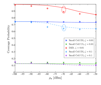
Figure 3: Comparison of D2D and small cell tier coverage probability from simulation (markers) and theoretical analysis (lines) as a function of $\rho_{\mathtt{s}}$, for $\lambda_{\mathtt{s}}=5\lambda_{\mathtt{m}}$, $\lambda_{\mathtt{u}}=100\lambda_{\mathtt{m}}$, $\{q_{\mathtt{D,m}},q_{\mathtt{D,s}}\}=\{0.5,0.5\}$, $\rho_{\mathtt{d}}=-60$ dBm, and $\{B_{\mathtt{D,m}},B_{\mathtt{D,s}},B_{\mathtt{U,m}},B_{\mathtt{U,s}}\}=\{1,1,1,1\}$.

In Fig. 3, we study the validity of the PPP approximation of active D2D transmitters in terms of coverage probability by varying $\rho_{\mathtt{s}}$. The approximation is caused by the following factors: (i) modeling the combined effect of PHP and MHP with an independent thinning of a PPP, (ii) neglecting the coupling between the locations of mobile users and base stations in the UL transmission, (iii) replacing the instantaneous exclusion distance by $\iota_{\mathtt{s}}$ and $\iota_{\mathtt{d}}$ constrained by a small miss detection probability threshold $\epsilon$. Figure 3 indicates that the PPP approximation is accurate for low and high values of $\rho_{\mathtt{s}}$. Low values of $\rho_{\mathtt{s}}$ correspond to large exclusion distances $\iota_{\mathtt{s}}$, leading to a low retaining probability $\beta$. The good agreement between simulation and analysis can be explained by the fact that the smaller density of D2D transmitters leads to little interference. For high values of $\rho_{\mathtt{s}}$ and corresponding small exclusion distances $\iota_{\mathtt{s}}$, the density of the active D2D transmitters approaches that of the initial PPP, which eliminates the inaccuracy caused by the approximation. The middle range of values of $\rho_{\mathtt{s}}$ results in inaccuracy on the coverage probability. Specifically, define the receiver sensitivity as $\rho_{\mathtt{min}}$, the extensive simulations show that the approximations are accurate (with the order of magnitude of the error less than 5%), when $\rho_{\mathtt{s}}\in[\rho_{\mathtt{min}},-95]\cup[-60,\infty)$ dBm, and reasonable (error order is within 10%) within the range $(-95,-60)$ dBm. In this example, the maximum error is achieved at $\rho_{\mathtt{s}}=-70$ dBm. However, the order of magnitude of the largest error is less than 10%. Similar effect can be seen for $\rho_{\mathtt{d}}$, and we find that the PPP approximation by varying $\rho_{\mathtt{d}}$ is more accurate than by varying $\rho_{\mathtt{s}}$. This can be explained by the larger effect of $\rho_{\mathtt{s}}$ on $\lambda_{\mathtt{d}}$ than the effect of $\rho_{\mathtt{d}}$ on $\lambda_{\mathtt{d}}$.

Figure 4 represents the coverage probability as a function of $q_{\mathtt{D,s}}$. We observe that the accuracy of the approximation deteriorates as more UL transmissions take place. For D2D users, the inaccuracy is mainly caused by the use of fixed $\iota_{\mathtt{s}}$, where the channel fading is averaged. Note that the D2D user coverage is dominated by the strong interference from DL active SAPs. As $q_{\mathtt{D,s}}$ increases, the density of DL SAPs increases and the impact of channel fading on the approximation is more apparent. To further verify the approximations, we perform extensive simulations by varying the related system parameters. Specifically, by increasing $\zeta$ or $\lambda_{\mathtt{s}}$, we observe a larger error of the approximation with regards to the D2D user coverage. In the worst case with $\zeta=0.9$, even in a sparse network scenario $\hat{\lambda}_{\mathtt{s}}^{(\mathtt{m})}=5$, the order of magnitude of the error can achieve 10%. While with a smaller D2D user fraction $\zeta=0.1$, the approximation can be accurate (error order is within 5%) in both sparse and moderate network scenario with $\hat{\lambda}_{\mathtt{s}}^{(\mathtt{m})}\leq 40$. However, in a very dense network scenario with $\hat{\lambda}_{\mathtt{s}}^{(\mathtt{m})}=100$, the order of magnitude of the error can be as large as 16%. The reasonable order of magnitude of the worst-case errors validates our theoretical model and in the following, we will present results based on our analytical framework.

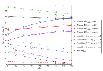
Figure 4: Comparison of coverage probability from simulation (markers) and theoretical analysis (lines) as a function of $q_{\mathtt{D},\mathtt{s}}$, ($\lambda_{\mathtt{s}}=5\lambda_{\mathtt{m}}$, $\lambda_{\mathtt{u}}=100\lambda_{\mathtt{m}}$, $\{B_{\mathtt{D,m}},B_{\mathtt{D,s}},B_{\mathtt{U,m}},B_{\mathtt{U,s}}\}=\{1,1,1,1\}$, $\zeta=0.1$, $\rho_{\mathtt{s}}=\rho_{\mathtt{d}}=-60$ dBm).

IV Coverage Probability Evaluation

In this section, we evaluate how the important network parameters, such as UL/DL configuration, base station density, and bias factor affect the load-aware coverage probability. In case of a fully-loaded network without D2D users, we derive the parameters that maximize the per tier coverage probability and overall coverage probability.

IV-A Effects of UL/DL configuration

In this section, we elucidate the non-trivial system behavior in dynamic TDD networks that results from the coexistence of UL and DL transmissions. How the UL/DL configuration $q_{\mathtt{D},i}$ affects $\mathbb{P}_{i}^{\mathtt{D}}$ and $\mathbb{P}_{i}^{\mathtt{U}}$ is not very explicit, because increasing $q_{\mathtt{D},i}$ gives rise to a reduction of the UL interference and a surge of the DL interference. However, for a given set of system parameters, we find for each tier $i$ that the relative transmit power $\frac{Q_{i}}{P_{i}}$ determines whether $\mathbb{P}_{i}^{\mathtt{D}}$ is dominated by the DL or the UL interference. According to this observation, in a fully-loaded network with $\rho_{\mathtt{s}}\rightarrow 0$, we derive the UL/DL configuration that optimizes the per tier coverage probability in DL and UL mode.

Optimization of per tier UL/DL configuration: In a fully-loaded network, i.e. $P_{e}^{\mathtt{D},k}\rightarrow 0$ and $P_{e}^{\mathtt{U},k}\rightarrow 0$, and for $\rho_{\mathtt{s}}\rightarrow 0$, the UL/DL configuration that maximizes the per tier UL coverage probability $\mathbb{P}_{\mathtt{m}}^{\mathtt{U}}$ and $\mathbb{P}_{\mathtt{s}}^{\mathtt{U}}$ is given by $q_{\mathtt{D,m}}^{\star\mathtt{U}}=0$ and $q_{\mathtt{D,s}}^{\star\mathtt{U}}=0$, respectively. The optimal UL/DL configuration for the per tier DL coverage probability is derived as follows. Define $\bar{q}_{\mathtt{D},k}=\hat{\lambda}_{i}^{(k)}\bigl{(}\hat{P}_{i}^{(k)}\hat{B}_{\mathtt{D},i}^{(k)}\bigr{)}^{\frac{2}{\alpha}}\Bigl{(}\frac{\delta\left(\gamma_{i}^{\mathtt{D}},\alpha\right)}{C(\alpha)\bigl{(}\frac{Q_{i}}{P_{i}}\gamma_{i}^{\mathtt{D}}\bigr{)}^{\frac{2}{\alpha}}}-1\Bigr{)}^{-1},\>k,i\in\{\mathtt{m},\mathtt{s}\},k\neq i.$

(i) If $\frac{\delta\left(\gamma_{i}^{\mathtt{D}},\alpha\right)}{C(\alpha)\bigl{(}\gamma_{i}^{\mathtt{D}}\bigr{)}^{\frac{2}{\alpha}}}\leq\bigl{(}\frac{Q_{i}}{P_{i}}\bigr{)}^{\frac{2}{\alpha}}$, $\mathbb{P}_{i}^{\mathtt{D}}$ is a monotone increasing function of $q_{\mathtt{D},i}$, where $\mathbb{P}_{i}^{\mathtt{D}}$ is dominated by the UL interference. The optimal UL/DL configuration is achieved at $q_{\mathtt{D,}i}^{\star\mathtt{D}}=1$;

(ii) If $\frac{\delta\left(\gamma_{i}^{\mathtt{D}},\alpha\right)}{C(\alpha)\bigl{(}\gamma_{i}^{\mathtt{D}}\bigr{)}^{\frac{2}{\alpha}}}>\bigl{(}\frac{Q_{i}}{P_{i}}\bigr{)}^{\frac{2}{\alpha}}$, the monotonicity of $\mathbb{P}_{i}^{\mathtt{D}}$ with respect to $q_{\mathtt{D},i}$ is determined by the range of $q_{\mathtt{D},k}$. When $q_{\mathtt{D},k}<\bar{q}_{\mathtt{D},k}$, $\mathbb{P}_{i}^{\mathtt{D}}$ increases with $q_{\mathtt{D},i}$, and we have $q_{\mathtt{D,}i}^{\star\mathtt{D}}=1$; when $q_{\mathtt{D},k}>\bar{q}_{\mathtt{D},k}$, $\mathbb{P}_{i}^{\mathtt{D}}$ is a decreasing function of $q_{\mathtt{D},i}$, where $\mathbb{P}_{i}^{\mathtt{D}}$ is dominated by the DL interference. The optimal UL/DL configuration is achieved at the limiting case of $q_{\mathtt{D,}i}^{\star\mathtt{D}}=0$.

The results can be obtained by taking the the first-order derivative of $\mathbb{P}_{i}^{\mathtt{D}}$ and $\mathbb{P}_{i}^{\mathtt{U}}$ with respect to $q_{\mathtt{D},i}$. In a realistic scenario, the base station has larger transmit power than that of mobile user, i.e., $P_{i}>Q_{i}$. Therefore, we have $\frac{\partial\mathbb{P}_{i}^{\mathtt{U}}}{\partial q_{\mathtt{D},i}}<0$, which means that $\mathbb{P}_{i}^{\mathtt{U}}$ decreases with $q_{\mathtt{D},i}$.

IV-B Effects of base station density

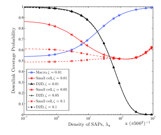
(a)

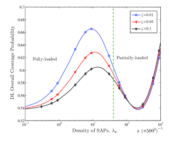
(b)

Figure 5: Downlink coverage probability vs. $\lambda_{\mathtt{s}}$, (a) for macro tier, small cell tier and D2D user, (b) for overall coverage of the infrastructure, ($\lambda_{\mathtt{m}}=\frac{1}{\pi 500^{2}}$, $\lambda_{\mathtt{u}}=10^{3}\lambda_{\mathtt{m}}$, $\{q_{\mathtt{D,m}},q_{\mathtt{D,s}}\}=\{0.5,0.5\}$, $\{B_{\mathtt{D,m}},B_{\mathtt{D,s}},B_{\mathtt{U,m}},B_{\mathtt{U,s}}\}=\{1,1,1,1\}$, $\rho_{\mathtt{s}}=\rho_{\mathtt{d}}=-60$ dBm).

From (LABEL:eq:macro_D) to (25) and the definition of $\mathcal{A}_{\mathtt{D},k}$ and $\mathcal{A}_{\mathtt{U},k}$, we observe that both the base station density and bias factor have similar effects on the coverage probability in DL and UL. Due to space limitations, we take DL coverage as an example and the conclusions can be directly applied to the UL case. We evaluate the variation of the DL load-aware coverage probability as a function of $\lambda_{\mathtt{s}}$, as depicted in Fig. 5. In terms of traffic load, the network evolves from a fully-loaded sparse network to a partially-loaded dense network. From Fig. 5(a), we observe that $\mathbb{P}_{\mathtt{m}}^{\mathtt{D}}$ increases monotonously with $\lambda_{\mathtt{s}}$, which can be ascribed to the handover of macro mobile users with low SIR to the small cell tier and the corresponding reduction of interference in the macro tier. With respect to the small cell tier, the small cell network interference increases with $\lambda_{\mathtt{s}}$, while the activity of D2D users diminishes exponentially with $\lambda_{\mathtt{s}}$ as can be verified in (18). These opposite effects are reflected in the load-aware coverage probability for the small cell tier. Figure 5(b) depicts the overall DL coverage probability $\bar{\mathbb{P}}_{\mathtt{D}}$ as a function of $\lambda_{\mathtt{s}}$ and indicates that an optimal $\lambda_{\mathtt{s}}$ can be found in the feasible region of small cell densities. As $\lambda_{\mathtt{s}}$ increases, the network load moves into the lightly loaded regime, where the aggregate small cell interference is constrained by the density of mobile users. As $\lambda_{\mathtt{s}}\rightarrow\infty$, we have $\mathcal{A}_{\mathtt{D},\mathtt{s}}\rightarrow 1$ and $\bar{\mathbb{P}}_{\mathtt{D}}\rightarrow 1$. As opposed to the fully-loaded traffic model with constant coverage probability in the asymptotic regime [29, 32], this result highlights the usefulness of the load-aware model to capture the coverage probability in realistic conditions. Given a good estimate of the user density, the proposed analytical framework allows us to find the small cell density within the realistic regime that optimizes the overall coverage probability. In the fully-loaded network and for $\rho_{\mathtt{s}}\rightarrow 0$, by taking the first-order derivative of $\bar{\mathbb{P}}_{\mathtt{D}}$ and $\bar{\mathbb{P}}_{\mathtt{U}}$ with respect to $\hat{\lambda}_{\mathtt{s}}^{(\mathtt{m})}$, the optimal relative base station density in DL mode $\hat{\lambda}_{\mathtt{s}}^{\mathtt{\left(m\right)\star D}}$ and UL mode $\hat{\lambda}_{\mathtt{s}}^{\mathtt{\left(m\right)\star U}}$ can be found as follows.

Optimization of base station density: In the fully-loaded network, the optimal $\hat{\lambda}_{\mathtt{s}}^{\mathtt{\left(m\right)\star D}}$ and $\hat{\lambda}_{\mathtt{s}}^{\mathtt{\left(m\right)\star U}}$ are given by

$$\hat{\lambda}_{\mathtt{s}}^{(\mathtt{m})\star\mathtt{D}}=\frac{q_{\mathtt{D,m}}P_{\mathtt{m}}^{\frac{2}{\alpha}}\delta(\gamma_{\mathtt{m}}^{\mathtt{D}},\alpha)+(1-q_{\mathtt{D},\mathtt{m}})\bigl{(}Q_{\mathtt{m}}\gamma_{\mathtt{m}}^{\mathtt{D}}\bigr{)}^{\frac{2}{\alpha}}}{\bigl{(}\hat{B}_{\mathtt{D,s}}^{(\mathtt{m})}\bigr{)}^{\frac{2}{\alpha}}\bigl{(}q_{\mathtt{D,s}}P_{\mathtt{s}}^{\frac{2}{\alpha}}\delta(\gamma_{\mathtt{s}}^{\mathtt{D}},\alpha)+(1-q_{\mathtt{D},\mathtt{s}})C(\alpha)\bigl{(}Q_{\mathtt{s}}\gamma_{\mathtt{s}}^{\mathtt{D}}\bigr{)}^{\frac{2}{\alpha}}\bigr{)}}$$ (35)

$$\hat{\lambda}_{\mathtt{s}}^{(\mathtt{m})\star\mathtt{U}}=\Bigl{(}\frac{\gamma_{\mathtt{m}}^{\mathtt{U}}}{\hat{B}_{\mathtt{U,s}}^{(\mathtt{m})}\gamma_{\mathtt{s}}^{\mathtt{U}}}\Bigr{)}^{\frac{2}{\alpha}}\cdot\frac{q_{\mathtt{D},\mathtt{m}}P_{\mathtt{m}}^{\frac{2}{\alpha}}+(1-q_{\mathtt{D},\mathtt{m}})Q_{\mathtt{m}}^{\frac{2}{\alpha}}}{q_{\mathtt{D},\mathtt{s}}P_{\mathtt{s}}^{\frac{2}{\alpha}}+(1-q_{\mathtt{D},\mathtt{s}})Q_{\mathtt{s}}^{\frac{2}{\alpha}}},$$ (36)

By analyzing the effect of key parameters, we can derive the following insights: (i) the optimal base station density $\hat{\lambda}_{\mathtt{s}}^{(\mathtt{m})\star\mathtt{D}}$ and $\hat{\lambda}_{\mathtt{s}}^{(\mathtt{m})\star\mathtt{U}}$ decreases with $\hat{B}_{\mathtt{D,s}}^{(\mathtt{m})}$ and $\hat{B}_{\mathtt{U,s}}^{(\mathtt{m})}$, respectively, (ii) for DL case, if $P_{\mathtt{m}}\gg Q_{\mathtt{m}}$ and $P_{\mathtt{s}}\gg Q_{\mathtt{s}}$, $\hat{\lambda}_{\mathtt{s}}^{(\mathtt{m})\star\mathtt{D}}\backsimeq\frac{q_{\mathtt{D,m}}P_{\mathtt{m}}^{\frac{2}{\alpha}}\delta\left(\gamma_{\mathtt{m}}^{\mathtt{D}},\alpha\right)}{q_{\mathtt{D,s}}\bigl{(}\hat{B}_{\mathtt{D,s}}^{(\mathtt{m})}\bigr{)}^{\frac{2}{\alpha}}P_{\mathtt{s}}^{\frac{2}{\alpha}}\delta\bigl{(}\gamma_{\mathtt{s}}^{\mathtt{D}},\alpha\bigr{)}}$, and we derive that $\hat{\lambda}_{\mathtt{s}}^{(\mathtt{m})\star\mathtt{D}}$ is proportional to $q_{\mathtt{D,m}}$ and inversely proportional to $q_{\mathtt{D,s}}$, (iii) for UL case, $\hat{\lambda}_{\mathtt{s}}^{(\mathtt{m})\star\mathtt{U}}$ increases with $q_{\mathtt{D,m}}$ while decreases with $q_{\mathtt{D,s}}$.

IV-C Effects of bias factor

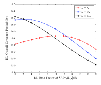
Figure 6: Overall downlink coverage probability as a function of DL bias factor of SAPs $B_{\mathtt{D,s}}$, ($\lambda_{\mathtt{u}}=10^{3}\lambda_{\mathtt{m}}$, $\{q_{\mathtt{D,m}},q_{\mathtt{D,s}}\}=\{0.5,0.5\}$, $\{B_{\mathtt{D,m}},B_{\mathtt{U,m}},B_{\mathtt{U,s}}\}=\{1,1,1\}$, $\zeta=0.01$, $\rho_{\mathtt{s}}=\rho_{\mathtt{d}}=-60$ dBm).

Figure 6 depicts the DL coverage probability as a function of the DL bias factor $B_{\mathtt{D,s}}$. We observe that increasing the density of SAPs $\lambda_{\mathtt{s}}$ decreases the optimal $B_{\mathtt{D,s}}$. This is due to the fact that a larger $\lambda_{\mathtt{s}}$ inflicts more interference on the small cell mobile users, and decreasing $B_{\mathtt{D,s}}$ helps to increase the overall coverage probability by shifting small cell mobile users with low SIR to the macro tier. It shows that with the analytical framework, we can derive the optimal $\hat{B}_{\mathtt{D,s}}^{(\mathtt{m})}$ and $\hat{B}_{\mathtt{U,s}}^{(\mathtt{m})}$ that maximize the overall coverage probability in DL and UL.

Optimization of bias factor: In the fully-loaded network, by taking the first-order derivative of $\bar{\mathbb{P}}_{\mathtt{D}}$ and $\bar{\mathbb{P}}_{\mathtt{U}}$ with respect to $\hat{B}_{\mathtt{D,s}}^{(\mathtt{m})}$ and $\hat{B}_{\mathtt{U,s}}^{(\mathtt{m})}$, we can derive the optimal $\hat{B}_{\mathtt{D,s}}^{(\mathtt{m})\star}$ and $\hat{B}_{\mathtt{U,s}}^{(\mathtt{m})\star}$ for DL and UL transmissions as

$$\hat{B}_{\mathtt{D,s}}^{(\mathtt{m})\star}=\Bigl{(}\frac{P_{\mathtt{m}}^{\frac{2}{\alpha}}q_{\mathtt{D,m}}\delta(\gamma_{\mathtt{m}}^{\mathtt{D}},\alpha)+(1-q_{\mathtt{D,m}})\bigl{(}Q_{\mathtt{m}}\gamma_{\mathtt{m}}^{\mathtt{D}}\bigr{)}^{\frac{2}{\alpha}}}{\hat{\lambda}_{\mathtt{s}}^{(\mathtt{m})}\bigl{(}P_{\mathtt{s}}^{\frac{2}{\alpha}}q_{\mathtt{D,s}}\delta(\gamma_{\mathtt{s}}^{\mathtt{D}},\alpha)+(1-q_{\mathtt{D,s}})C(\alpha)\bigl{(}Q_{\mathtt{s}}\gamma_{\mathtt{s}}^{\mathtt{D}}\bigr{)}^{\frac{2}{\alpha}}\bigr{)}}\Bigr{)}^{\frac{\alpha}{2}}$$ (37)

$$\hat{B}_{\mathtt{U,s}}^{(\mathtt{m})\star}=\Bigl{(}\frac{\bigl{(}\gamma_{\mathtt{m}}^{\mathtt{U}}\bigr{)}^{\frac{2}{\alpha}}\bigl{(}q_{\mathtt{D,m}}P_{\mathtt{m}}^{\frac{2}{\alpha}}+(1-q_{\mathtt{D,m}})Q_{\mathtt{m}}^{\frac{2}{\alpha}}\bigr{)}}{\hat{\lambda}_{\mathtt{s}}^{(\mathtt{m})}\bigl{(}\gamma_{\mathtt{s}}^{\mathtt{U}}\bigr{)}^{\frac{2}{\alpha}}\bigl{(}q_{\mathtt{D,s}}P_{\mathtt{s}}^{\frac{2}{\alpha}}+(1-q_{\mathtt{D,s}})Q_{\mathtt{s}}^{\frac{2}{\alpha}}\bigr{)}}\Bigr{)}^{\frac{\alpha}{2}}.$$ (38)

V Network Access Design

In this section, we first study the D2D enhanced network from a throughput perspective and demonstrate the substantial throughput gain achieved by D2D transmissions. Then we investigate the network access scheme both from a coverage and throughput perspective. To emphasize the benefit of network access scheme, we compare the proposed CSMA scheme with the random access scheme ALOHA.

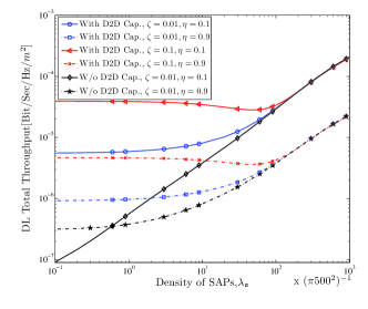
Figure 7: Downlink total throughput vs. $\lambda_{\mathtt{s}}$ ($\lambda_{\mathtt{u}}=10^{3}\lambda_{\mathtt{m}}$, $\{q_{\mathtt{D,m}},q_{\mathtt{D,s}}\}=\{0.5,0.5\}$, $\{B_{\mathtt{D,m}},B_{\mathtt{D,s}},B_{\mathtt{U,m}},B_{\mathtt{U,s}}\}=\{1,1,1,1\}$, $\rho_{\mathtt{s}}=\rho_{\mathtt{d}}=-60$ dBm).

Figure 7 presents the DL network throughput with and without D2D capabilities as a function of $\lambda_{\mathtt{s}}$ for different values of the bandwidth partition factor $\eta$. Without D2D capabilities, the potential D2D transmitters can only associate with the infrastructure in UL, and those potential D2D receivers are blocked in the current timeslot. Comparing the curves with and without D2D capabilities for the same $\zeta$, we observe that even a small D2D user fraction ($\zeta=0.01$) results in a considerable throughput gain. In the D2D enhanced network, we observe that allocating more spectrum to the small cell tier leads to a larger network throughput, ascribed to the high outage capacity of D2D users and the spatial reuse gain from small cell transmissions. Figure 7 also illustrates that the network throughput benefits from a higher fraction of potential D2D users $\zeta$. Interestingly, the network throughput with $\zeta=0.1$ features a convex behavior as a function of $\lambda_{\mathtt{s}}$. The initial decrease of network throughput follows from the decline of the retaining probability with $\lambda_{\mathtt{s}}$ as indicated in (18). Compared with Fig. 5, we also observe that the D2D user fraction $\zeta$ leads to a tradeoff between the overall coverage probability and the total network throughput for fully-loaded network. A larger $\zeta$ improves the network throughput, yet deteriorates the overall coverage probability due to the interference inflicted on the small cell tier. The results presented in Fig. 7 indicate that the bandwidth partition strongly affects the network throughput. In the following, we derive the optimal bandwidth partition factor $\eta^{\star}$ by taking the DL network throughput presented in (33) as an example.

Optimization of bandwidth partition: If $\mathcal{T}_{\mathtt{m}}^{\mathtt{D}}>\mathcal{T}_{\mathtt{s}}^{\mathtt{D}}+\frac{1}{2}\mathcal{T}_{\mathtt{d}}$, $\mathcal{T}_{\mathtt{D}}(\eta;\rho_{\mathtt{s}};\rho_{\mathtt{d}})$ is a monotone increasing function of $\eta$, we have $\eta^{\star}=1$ and $\mathcal{T}_{\mathtt{D}}^{\star}(\eta^{\star};\rho_{\mathtt{s}};\rho_{\mathtt{d}})=\mathcal{T}_{\mathtt{m}}^{\mathtt{D}}$; if $\mathcal{T}_{\mathtt{m}}^{\mathtt{D}}<\mathcal{T}_{\mathtt{s}}^{\mathtt{D}}+\frac{1}{2}\mathcal{T}_{\mathtt{d}},$ $\mathcal{T}_{\mathtt{D}}(\eta;\rho_{\mathtt{s}};\rho_{\mathtt{d}})$ monotonously decreases with $\eta$, thereby $\eta^{\star}=0$ and $\mathcal{T}_{\mathtt{D}}^{\star}(\eta^{\star};\rho_{\mathtt{s}};\rho_{\mathtt{d}})=\mathcal{T}_{\mathtt{s}}^{\mathtt{D}}+\frac{1}{2}\mathcal{T}_{\mathtt{d}}$; if $\mathcal{T}_{\mathtt{m}}^{\mathtt{D}}=\mathcal{T}_{\mathtt{s}}^{\mathtt{D}}+\frac{1}{2}\mathcal{T}_{\mathtt{d}}$, $\mathcal{T}_{\mathtt{D}}(\eta;\rho_{\mathtt{s}};\rho_{\mathtt{d}})$ is a constant and does not change with $\eta$. The result is intuitive, which means giving more bandwidth to the dominant tier is beneficial to the total network throughput.

In this work, we use the distributed network access scheme CSMA to control the channel access of D2D transmitters and protect the ongoing small cell transmissions. We study the network access scheme both from a coverage and throughput perspective. We refer to Fig. 3, which depicts that both the coverage probabilities of small cell tier and D2D user deteriorate with $\rho_{\mathtt{s}}$. Similar effect can be seen for $\rho_{\mathtt{d}}$. This is due to the fact that the retaining probability and corresponding $\lambda_{\mathtt{d}}$ increase with $\rho_{\mathtt{s}}$ and $\rho_{\mathtt{d}}$. Thus, in terms of the overall coverage probability for infrastructure based transmissions and typical D2D user, the optimal sensing threshold is given by $\rho_{\mathtt{s}}^{\star}=0$ and $\rho_{\mathtt{d}}^{\star}=0$. However, the absence of D2D transmissions results in reduced network throughput.

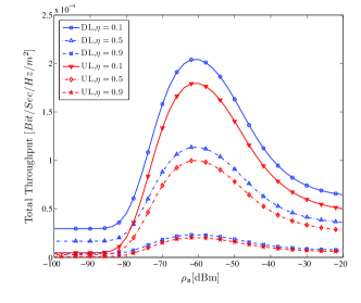
(a)

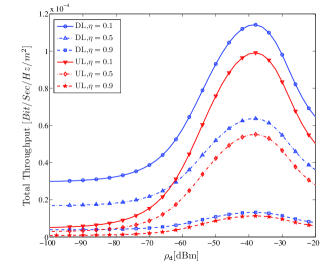
(b)

Figure 8: Total network throughput vs. protection threshold $\rho_{\mathtt{s}}$ or contention threshold $\rho_{\mathtt{d}}$, (a) for $\rho_{\mathtt{s}}$, with $\rho_{\mathtt{d}}=-20$ dBm, (b) for $\rho_{\mathtt{d}}$, with $\rho_{\mathtt{s}}=-20$ dBm, ($\lambda_{\mathtt{u}}=10^{4}\lambda_{\mathtt{m}}$, $\lambda_{\mathtt{s}}=100\lambda_{\mathtt{m}}$, $\{q_{\mathtt{D,m}},q_{\mathtt{D,s}}\}=\{0.5,0.5\}$, $\zeta=0.1$).

Figure 8 depicts the total network throughput as a function of $\rho_{\mathtt{s}}$ and $\rho_{\mathtt{d}}$. From Fig. 8(a), we observe that the network throughput exhibits a concave behavior with respect to $\rho_{\mathtt{s}}$. This is caused by the opposite effects of $\rho_{\mathtt{s}}$ on $\lambda_{\mathtt{d}}$ and the coverage probability of the small cell tier and typical D2D user, a tradeoff between coverage probability and D2D user activity that is made explicit in the expressions of the network throughput (33) and (34). From Fig. 8(b), we notice a similar effect of $\rho_{\mathtt{d}}$ on the network throughput. As for the coverage analysis, the effect of $\rho_{\mathtt{s}}$ on the network throughput is more evident than the effect of $\rho_{\mathtt{d}}$. This can be understood by the effectiveness of the protection threshold $\rho_{\mathtt{s}}$ in controlling the mutual interference and improving the coverage probability. In addition, we observe that the optimal $\rho_{\mathtt{d}}^{\star}$ is larger than $\rho_{\mathtt{s}}^{\star}$ due to the smaller effect of $\rho_{\mathtt{d}}$ on the D2D retaining probability $\beta$. Figure 8 also shows that in the dense scenario ($\lambda_{\mathtt{s}}=100\lambda_{\mathtt{m}}$), giving more bandwidth to the small cell tier can increase the total network throughput. The presented results show that the proposed analytical framework can be used to determine $\rho_{\mathtt{s}}^{\star}$ or $\rho_{\mathtt{d}}^{\star}$ that maximize the total network throughput.

In Fig. 9, we depict the coverage probability and DL network throughput as a function of retaining probability $\beta$ or access probability $p$ when D2D users utilize CSMA and ALOHA. We keep $\rho_{\mathtt{d}}=-20$ dBm, and change $\rho_{\mathtt{s}}$ to alter $\beta$. With ALOHA, each D2D transmitter activates its transmission with a certain probability $p$, $p\in(0,1]$, such that the active D2D transmitters form a PPP with density $p\lambda_{\mathtt{d}}$. To make a fair comparison, let $p=\beta$. From Fig. 9(a) and Fig. 9(b), we observe that the proposed CSMA scheme has prominent advantage over ALOHA in both coverage probability and network throughput, which indicates that better network performance can be achieved by a careful network access design.

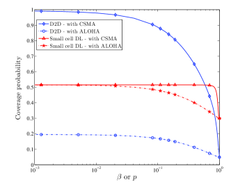
(a)

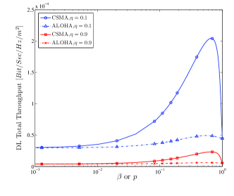
(b)

Figure 9: Comparison of coverage probability and DL total network throughput from CSMA and ALOHA as a function of retaining probability $\beta$ or access probability $p$, (a) for coverage probability, (b) for downlink total network throughput, ($\lambda_{\mathtt{u}}=10^{4}\lambda_{\mathtt{m}}$, $\lambda_{\mathtt{s}}=100\lambda_{\mathtt{m}}$, $\{q_{\mathtt{D,m}},q_{\mathtt{D,s}}\}=\{0.5,0.5\}$, $\zeta=0.1$, $\rho_{\mathtt{d}}=-20$ dBm).

Optimization of $\rho_{\mathtt{s}}$ and $\rho_{\mathtt{d}}$: The optimal sensing thresholds have been determined by using a numerical search with limited computational complexity. We take the DL total throughput derived in (33) as an example. Since $\mathcal{T}_{\mathtt{D}}(\eta;\rho_{\mathtt{s}};\rho_{\mathtt{d}})$ is a continuous function of $\rho_{\mathtt{s}}$ over [0,$\infty$], there exists at least one optimal $\rho_{\mathtt{s}}^{\star}$ where $\mathcal{T}_{\mathtt{D}}(\eta;\rho_{\mathtt{s}};\rho_{\mathtt{d}})$ is maximized. Considering the signal attenuation characteristics, $\rho_{\mathtt{s}}^{\star}$ is upper bounded by the transmit power of D2D user $Q_{\mathtt{d}}$. Therefore, we have $\rho_{\mathtt{s}}^{\star}\in[0,Q_{\mathtt{d}}]$, which reduces the complexity of the search process. Similarly, we can get $\rho_{\mathtt{d}}^{\star}\in[0,Q_{\mathtt{d}}]$. The joint optimization of $\rho_{\mathtt{s}}$ and $\rho_{\mathtt{d}}$ may be implemented with a two-stage optimization method where we first fix $\rho_{\mathtt{d}}$ and optimize the network throughput with respect to $\rho_{\mathtt{s}}$, followed by the optimization with respect to $\rho_{\mathtt{d}}$.

VI Conclusion

In this work, we studied a two-tier D2D enhanced HCN operating with dynamic TDD, where the D2D transmitters follow a CSMA scheme. We proposed a simple PPP model for the active D2D users and verified the accuracy by extensive simulations. We presented an analytical framework to evaluate the load-aware coverage probability and network throughput. The proposed model allows us to analyze the non-trivial system behavior of dynamic TDD networks and to quantify the effect of most important network parameters such as the UL/DL configuration, base station density, and bias factor on the coverage probability, and the bandwidth partition on the total network throughput. We provided guidelines on the optimal design of the network access scheme. Possible future directions to extend this work are to include a dynamic traffic model in our framework and consider the spatio-temporal correlations in the dynamic TDD network.

A. Proof of Lemma 2

Assuming $T_{0}$ locates at the origin and by Slivnyak’s Theorem, the point process of the D2D contenders forms a PPP. By using the Palm distribution $P_{0}$, we derive the retaining probability $\beta$ of a potential D2D transmitter as follows:

$$\beta = P_{0}[U_{0}=1]$$

$$= \mathbb{E}_{0}\Bigl{[}\prod_{Y_{j}\in\Phi_{\mathtt{s}}^{\mathtt{D}}}\mathbf{1}_{\bigl{(}\frac{Q_{\mathtt{d}}h_{oj}}{\|T_{0}-Y_{j}\|^{\alpha}}<\rho_{\mathtt{s}}\bigr{)}}\prod_{Z_{l}\in\Phi_{\mathtt{u},\mathtt{s}}^{\mathtt{T}}}\mathbf{1}_{\bigl{(}\frac{Q_{\mathtt{d}}h_{ol}}{\|T_{0}-Z_{l}\|^{\alpha}}<\rho_{\mathtt{s}}\bigr{)}}$$

$$\times\prod_{T_{k}\in\Phi_{\mathtt{d}}\backslash T_{0}}\bigl{(}\mathbf{1}_{(t_{0}\leq t_{k})}+\mathbf{1}_{(t_{0}>t_{k})}\mathbf{1}_{\bigl{(}\frac{Q_{\mathtt{d}}h_{ok}}{\|T_{0}-T_{k}\|^{\alpha}}<\rho_{\mathtt{d}}\bigr{)}}\bigr{)}\Bigr{]}$$

$$\overset{(a)}{=} \mathbb{E}_{0}\Bigl{[}\prod_{Y_{j}\in\Phi_{\mathtt{s}}^{\mathtt{D}}}\bigl{(}1-e^{-\frac{\rho_{\mathtt{s}}}{Q_{\mathtt{d}}}\|Y_{j}\|^{\alpha}}\bigr{)}\Bigr{]}\mathbb{E}_{0}\Bigl{[}\prod_{Z_{l}\in\Phi_{\mathtt{u},\mathtt{s}}^{\mathtt{T}}}\bigl{(}1-e^{-\frac{\rho_{\mathtt{s}}}{Q_{\mathtt{d}}}\|Z_{l}\|^{\alpha}}\bigr{)}\Bigr{]}$$

$$\times\int_{0}^{1}\mathbb{E}_{0}\Bigl{[}\prod_{T_{k}\in\Phi_{\mathtt{d}}\backslash T_{0}}\mathbb{E}\bigl{[}\left(1-t\right)+t\bigl{(}1-e^{-\frac{\rho_{\mathtt{d}}}{Q_{\mathtt{d}}}\|T_{k}\|^{\alpha}}\bigr{)}\bigr{]}\Bigr{]}dt$$

$$\overset{(b)}{=} \exp\bigl{(}-\lambda_{\mathtt{s}}^{\mathtt{D}}\int_{\mathbb{R}^{2}}e^{-\frac{\rho_{\mathtt{s}}}{Q_{\mathtt{d}}}\|x\|^{\alpha}}dx\bigr{)}\exp\bigl{(}-\lambda_{\mathtt{u,s}}^{\mathtt{T}}\int_{\mathbb{R}^{2}}e^{-\frac{\rho_{\mathtt{s}}}{Q_{\mathtt{d}}}\|x\|^{\alpha}}dx\bigr{)}$$

$$\times\int_{0}^{1}\exp\bigl{(}-\zeta\lambda_{\mathtt{u}}t\int_{\mathbb{R}^{2}}e^{-\frac{\rho_{\mathtt{d}}}{Q_{\mathtt{d}}}\|x\|^{\alpha}}dx\bigr{)}dt$$

$$\overset{\left(c\right)}{=} \exp\bigl{(}-\bigl{(}\lambda_{\mathtt{s}}^{\mathtt{D}}+\lambda_{\mathtt{u,s}}^{\mathtt{T}}\bigr{)}\mathcal{K}_{o,\mathtt{s}}\bigr{)}\frac{1-\exp\bigl{(}-\zeta\lambda_{\mathtt{u}}\mathcal{K}_{o,\mathtt{d}}\bigr{)}}{\zeta\lambda_{\mathtt{u}}\mathcal{K}_{o,\mathtt{d}}},$$

where $\mathcal{K}_{o,\mathtt{s}}=\frac{2\pi\Gamma\left(\frac{2}{\alpha}\right)}{\alpha\bigl{(}\frac{\rho_{\mathtt{s}}}{Q_{\mathtt{d}}}\bigr{)}^{\frac{2}{\alpha}}}$ and $\mathcal{K}_{o,\mathtt{d}}=\frac{2\pi\Gamma\left(\frac{2}{\alpha}\right)}{\alpha\bigl{(}\frac{\rho_{\mathtt{d}}}{Q_{\mathtt{d}}}\bigr{)}^{\frac{2}{\alpha}}}$, (a) follows by the independence of PPPs and the expectation over the channel gains $h$, (b) is obtained by using the probability generating functional (PGFL) of the PPP [13] of $\Phi_{\mathtt{s}}^{\mathtt{D}}$, $\Phi_{\mathtt{u,s}}^{\mathtt{T}}$ and $\Phi_{\mathtt{d}}$, and (c) evaluates the given integrals by changing to polar coordinates and the use of Gamma function.

B. Proof of Theorem 1

First, we derive the coverage probability of the macro tier as follows. For DL mode,

$$\mathbb{P}_{\mathtt{m}}^{\mathtt{D}}$$

$$\overset{(a)}{=} \int_{0}^{\infty}\mathbb{E}_{\Phi_{\mathtt{m}}^{\mathtt{D}},\Phi_{\mathtt{u},\mathtt{m}}^{\mathtt{T}}}\Bigl{[}\exp\bigl{(}-\frac{\gamma_{\mathtt{m}}^{\mathtt{D}}r^{\alpha}}{P_{\mathtt{m}}}\bigl{(}I_{\mathtt{D\rightarrow D}}^{\mathtt{(m)}}+I_{\mathtt{U\rightarrow D}}^{\mathtt{(m)}}\bigr{)}\bigr{)}\Bigr{]}f_{Y_{\mathtt{D,m}}}\left(r\right)dr$$

$$\overset{(b)}{=} \int_{0}^{\infty}\mathbb{E}_{\Phi_{\mathtt{m}}^{\mathtt{D}}}\Bigl{[}\exp\Bigl{(}-\frac{\gamma_{\mathtt{m}}^{\mathtt{D}}r^{\alpha}}{P_{\mathtt{m}}}I_{\mathtt{D\rightarrow D}}^{\mathtt{(m)}}\Bigr{)}\Bigr{]}$$

$$\times\mathbb{E}_{\Phi_{\mathtt{u,m}}^{\mathtt{T}}}\Bigl{[}\exp\Bigl{(}-\frac{\gamma_{\mathtt{m}}^{\mathtt{D}}r^{\alpha}}{P_{\mathtt{m}}}I_{\mathtt{U\rightarrow D}}^{\mathtt{(m)}}\Bigr{)}\Bigr{]}f_{Y_{\mathtt{D,m}}}\left(r\right)dr$$

$$\overset{(c)}{=} \int_{0}^{\infty}\exp\left(-\pi r^{2}\lambda_{\mathtt{m}}^{\mathtt{D}}\delta\left(\gamma_{\mathtt{m}}^{\mathtt{D}},\alpha\right)\right)$$

$$\times\exp\biggl{(}-\pi r^{2}\lambda_{\mathtt{u,m}}^{\mathtt{T}}C\left(\alpha\right)\Bigl{(}\frac{Q_{\mathtt{m}}}{P_{\mathtt{m}}}\gamma_{\mathtt{m}}^{\mathtt{D}}\Bigr{)}^{{}^{\frac{2}{\alpha}}}\biggr{)}f_{Y_{\mathtt{D,m}}}\left(r\right)dr$$

$$\overset{(d)}{=} \frac{q_{\mathtt{D,m}}\lambda_{\mathtt{m}}}{\lambda_{\mathtt{m}}^{\mathtt{D}}\mathcal{A}_{\mathtt{D}\mathtt{,m}}\delta\left(\gamma_{\mathtt{m}}^{\mathtt{D}},\alpha\right)+\lambda_{\mathtt{u,m}}^{\mathtt{T}}\mathcal{A}_{\mathtt{D}\mathtt{,m}}C\left(\alpha\right)\bigl{(}\frac{Q_{\mathtt{m}}\gamma_{\mathtt{m}}^{\mathtt{D}}}{P_{\mathtt{m}}}\bigr{)}^{\frac{2}{\alpha}}+q_{\mathtt{D,m}}\lambda_{\mathtt{m}}},$$

where $C\left(\alpha\right)=\frac{2\pi/\alpha}{\sin\left(2\pi/\alpha\right)}$, and $\delta\left(\beta,\alpha\right)=\int_{\beta^{-\frac{2}{\alpha}}}^{\infty}\frac{\beta^{\frac{2}{\alpha}}}{1+u^{\frac{\alpha}{2}}}du$, (a) follows by taking expectation over the channel gains $h$, (b) is due to the independence of the PPPs, (c) results from the Laplace transform, where the first exponential term is caused by the fact that the active interfering MBSs can not stay within the disk $b\left(0,r\right)$. Finally, (d) follows by integrating with respect to the PDF $f_{Y_{\mathtt{D},\mathtt{m}}}(y)$ as defined in (13). For UL mode, the coverage probability is given by

$$\mathbb{P}_{\mathtt{m}}^{\mathtt{U}}$$

$$= \int_{0}^{\infty}\mathbb{E}_{\Phi_{\mathtt{m}}^{\mathtt{D}},\Phi_{\mathtt{u},\mathtt{m}}^{\mathtt{T}}}\Bigl{[}\exp\bigl{(}-\frac{\gamma_{\mathtt{m}}^{\mathtt{U}}r^{\alpha}}{Q_{\mathtt{m}}}\bigl{(}I_{\mathtt{D\rightarrow U}}^{\mathtt{(m)}}+I_{\mathtt{U\rightarrow U}}^{(\mathtt{m})}\bigr{)}\bigr{)}\Bigr{]}f_{Y_{\mathtt{U},\mathtt{m}}}\left(r\right)dr$$

$$= \int_{0}^{\infty}\exp\bigl{(}-\pi r^{2}\lambda_{\mathtt{m}}^{\mathtt{D}}C\left(\alpha\right)\bigl{(}\frac{P_{\mathtt{m}}}{Q_{\mathtt{m}}}\gamma_{\mathtt{m}}^{\mathtt{U}}\bigr{)}^{\frac{2}{\alpha}}\bigr{)}$$

$$\times\exp\bigl{(}-\pi r^{2}\lambda_{\mathtt{u,m}}^{\mathtt{T}}C\left(\alpha\right)\left(\gamma_{\mathtt{m}}^{\mathtt{U}}\right)^{\frac{2}{\alpha}}\bigr{)}f_{Y_{\mathtt{U},\mathtt{m}}}\left(r\right)dr$$

$$= \frac{(1-q_{\mathtt{D,m}})\lambda_{\mathtt{m}}}{C\left(\alpha\right)\bigl{(}\gamma_{\mathtt{m}}^{\mathtt{U}}\bigr{)}^{\frac{2}{\alpha}}\mathcal{A}_{\mathtt{U}\mathtt{,m}}\bigl{(}\lambda_{\mathtt{m}}^{\mathtt{D}}\bigl{(}\frac{P_{\mathtt{m}}}{Q_{\mathtt{m}}}\bigr{)}^{\frac{2}{\alpha}}+\lambda_{\mathtt{u,m}}^{\mathtt{T}}\bigr{)}+(1-q_{\mathtt{D,m}})\lambda_{\mathtt{m}}}.$$

With regard to the small cell tier, the Laplace transform of the aggregate interference from active SAPs and transmitting mobile users can be derived similar to (LABEL:eq:Cov_dm) and (LABEL:eq:Cov_um), respectively. In the following, we focus on the Laplace transform of the aggregate interference from active D2D transmitters. As is shown in Fig. 2, we have

$$\mathcal{L}_{I}(s) = \mathbb{E}_{\Phi_{\mathtt{d}}}\Biggl{[}\exp\biggl{(}-s\Bigl{(}\sum_{z\in\Phi_{\mathtt{d}}\cap\overline{\mathcal{H}}}Q_{\mathtt{d}}h_{oz}z^{-\alpha}\Bigr{)}\biggr{)}\Biggr{]}$$ (41)

$$\times \mathbb{E}_{\Phi_{\mathtt{d}}}\Biggl{[}\exp\biggl{(}-s\Bigl{(}\sum_{z\in\Phi_{\mathtt{d}}\cap\mathcal{H}\cap\overline{\mathcal{B}}}Q_{\mathtt{d}}h_{oz}z^{-\alpha}\Bigr{)}\biggr{)}\Biggr{]}$$

where the first term is related to the interferer distributed outside the big circle of radius $\|y_{0}\|+\iota_{\mathtt{s}}$, i.e. the shaded region $\Phi_{\mathtt{d}}\cap\overline{\mathcal{H}}$ , and can be easily derived. The second term corresponds to the interferer scattered over the shaded region within the big circle, i.e. $\Phi_{\mathtt{d}}\cap\mathcal{H}\cap\overline{\mathcal{B}}$. Two cases are differentiated for the calculation of the Laplace transform: $\|y_{0}\|\leq\iota_{\mathtt{s}}$ (see Fig. 2(a)) and $\|y_{0}\|>\iota_{\mathtt{s}}$ (see Fig. 2(b)). Denote the Laplace transform of the interference from active D2D transmitters in $\Phi_{\mathtt{d}}\cap\overline{\mathcal{H}}$ and $\Phi_{\mathtt{d}}\cap\mathcal{H}\cap\overline{\mathcal{B}}$ as $\mathcal{L}_{I_{out}}(s)$ and $\mathcal{L}_{I_{in}}(s)$, respectively. Conditioned on the typical small cell link length being $\|y_{0}\|$, we have

$$\mathcal{L}_{I_{out}}(s\mid\|y_{0}\|)$$ (42)

$$= \mathbb{E}_{\Phi_{\mathtt{d}}}\Biggl{[}\exp\biggl{(}-s\Bigl{(}\sum_{z\in\Phi_{\mathtt{d}}\cap\overline{\mathcal{H}}}Q_{\mathtt{d}}h_{oz}z^{-\alpha}\Bigr{)}\biggr{)}\mid\|y_{0}\|\Biggr{]}$$

$$\overset{(a)}{=} \exp\Bigl{(}-2\pi\lambda_{\mathtt{d}}\int_{\iota_{\mathit{\mathtt{s}}+\|y_{0}\|}}^{\infty}\frac{y}{1+\frac{y^{\alpha}}{sQ_{\mathtt{d}}}}dy\Bigr{)}$$

$$\overset{(b)}{=} \exp\Bigl{(}-\pi\lambda_{\mathtt{d}}\bigl{(}\iota_{\mathtt{s}}+\|y_{0}\|\bigr{)}^{2}\delta\Bigl{(}\frac{sQ_{\mathtt{d}}}{\bigl{(}\iota_{\mathtt{s}}+\|y_{0}\|\bigr{)}^{\alpha}},\alpha\Bigr{)}\Bigr{)}$$

where (a) follows from the PGFL of the PPP, and (b) is due to $\delta\left(\beta,\alpha\right)=\int_{\beta^{-\frac{2}{\alpha}}}^{\infty}\frac{\beta^{\frac{2}{\alpha}}}{1+u^{\frac{2}{\alpha}}}du$, with $\iota_{\mathtt{s}}+\|y_{0}\|$ denoting the distance from the nearest interferer staying within $\Phi_{\mathtt{d}}\cap\overline{\mathcal{H}}$.

In the following, we focus on the computation of $\mathcal{L}_{I_{in}}(s)$. For notational simplicity, we first define a $\mathcal{Z}$ function as

$$\mathcal{Z}_{\theta_{l},\kappa_{l}}^{\theta_{u},\kappa_{u}}\left(s;Q\right)=\left(sQ\right)^{\frac{2}{\alpha}}\int_{\theta_{l}}^{\theta_{u}}\int_{\frac{\kappa_{l}^{2}}{(sQ)^{\frac{2}{\alpha}}}}^{\frac{\kappa_{u}^{2}}{\left(sQ\right)^{\frac{2}{\alpha}}}}\frac{1}{1+u^{\frac{2}{\alpha}}}dud\theta,$$ (43)

where $Q$ represents the transmit power of interferer, $\theta_{l}$, $\theta_{u}$, and $\kappa_{l}$, $\kappa_{u}$ denote the lower bound and upper bound of the angle and distance from the interferer distributed in the shaded region $\Phi_{\mathtt{d}}\cap\mathcal{H}\cap\overline{\mathcal{B}}$.

For $\|y_{0}\|\leq\iota_{\mathtt{s}}$, denote $l_{OA}=||OA||$, we have $l_{OA}=\sqrt{\iota_{\mathtt{s}}^{2}-\bigl{(}\|y_{0}\|\textrm{sin}\theta\bigr{)}^{2}}+\|y_{0}\|\cos\theta,\;\theta\in[0,\pi].$ The Laplace transform $\mathcal{L}_{I_{in}}(s\mid\|y_{0}\|\leq\iota_{\mathtt{s}})$ is derived as

$$\mathcal{L}_{I_{in}}(s\mid\|y_{0}\|\leq\iota_{\mathtt{s}})$$ (44)

$$= \mathbb{E}_{\Phi_{\mathtt{d}}}\Bigl{[}\exp\bigl{(}-s(\sum_{z\in\Phi_{\mathtt{d}}\cap\mathcal{H}\cap\overline{\mathcal{B}}}Q_{\mathtt{d}}h_{oz}z^{-\alpha})\bigr{)}\mid\|y_{0}\|\leq\iota_{\mathtt{s}}\Bigr{]}$$

$$\overset{(a)}{=} \exp\bigl{(}-2\lambda_{\mathtt{d}}\int_{0}^{\pi}\int_{l_{OA}}^{\iota_{\mathtt{s}}+\|y_{0}\|}\frac{y}{1+\frac{y^{\alpha}}{sQ_{\mathtt{d}}}}dyd\theta\bigr{)}$$

$$\overset{(b)}{=} \exp\Bigl{(}-\lambda_{\mathtt{d}}\mathcal{Z}_{0,l_{OA}}^{\pi,\iota_{s}+\|y_{0}\|}\left(s;Q_{\mathtt{d}}\right)\Bigr{)},$$

where (a) follows by the PGFL of the PPP and by converting to polar coordinates, and (b) follows by substituting the corresponding bounds of the angle and distance into (43). By combining (42) with (44), we have

$$\mathcal{L}_{I}(s\mid\|y_{0}\|\leq\iota_{\mathtt{s}})=\mathcal{L}_{I_{out}}(s\mid\|y_{0}\|)\mathcal{L}_{I_{in}}(s\mid\|y_{0}\|\leq\iota_{\mathtt{s}}).$$ (45)

For $\|y_{0}\|>\iota_{\mathtt{s}}$, denote $\Theta=\arcsin\bigl{(}\frac{\iota_{\mathtt{s}}}{\|y_{0}\|}\bigr{)}$, $l_{OD}=\|OD\|$ and $l_{OC}=||OC||$, where $l_{OD}$ and $l_{OC}$ can be found by simple geometric formulas, similar to $l_{OA}$ given before. The Laplace transform $\mathcal{L}_{I_{in}}(s\mid\|y_{0}\|>\iota_{\mathtt{s}})$ is given by

$$\mathcal{L}_{I_{in}}(s\mid\|y_{0}\|>\iota_{\mathtt{s}})$$ (46)

$$\overset{(a)}{=} \exp\Bigl{(}-2\lambda_{\mathtt{d}}\bigl{(}\int_{0}^{\Theta}\int_{0}^{l_{OD}}\frac{y}{1+\frac{y^{\alpha}}{sQ_{\mathtt{d}}}}dyd\theta+\int_{0}^{\Theta}\int_{l_{OC}}^{\iota_{\mathtt{s}}+\|y_{0}\|}$$

$$\times\frac{y}{1+\frac{y^{\alpha}}{sQ_{\mathtt{d}}}}dyd\theta+\int_{\Theta}^{\pi}\int_{0}^{\iota_{\mathtt{s}}+\|y_{0}\|}\frac{y}{1+\frac{y^{\alpha}}{sQ_{\mathtt{d}}}}dyd\theta\bigr{)}\Bigr{)}$$

$$= \exp\Bigl{(}-\lambda_{\mathtt{d}}\bigl{(}\mathcal{Z}_{0,0}^{\Theta,l_{OD}}\left(s;Q_{\mathtt{d}}\right)$$

$$+\mathcal{Z}_{0,l_{OC}}^{\Theta,\iota_{\mathtt{s}}+\|y_{0}\|}\left(s;Q_{\mathtt{d}}\right)+\mathcal{Z}_{\Theta,0}^{\pi,\iota_{\mathtt{s}}+\|y_{0}\|}\left(s;Q_{\mathtt{d}}\right)\bigr{)}\Bigr{)},$$

where (a) is due to the fact that when $\theta<\arcsin\bigl{(}\frac{\iota_{\mathtt{s}}}{\|y_{0}\|}\bigr{)}$, the line $\overline{OB}$ shown in Fig. 2(b) passes through the whole exclusion region. By combining (42) with (46), we obtain

$$\mathcal{L}_{I}(s\mid\|y_{0}\|>\iota_{\mathtt{s}})=\mathcal{L}_{I_{out}}(s\mid\|y_{0}\|)\mathcal{L}_{I_{in}}(s\mid\|y_{0}\|>\iota_{\mathtt{s}}).$$ (47)

For DL transmission, substituting $I=I_{\mathtt{d\rightarrow D}}=\sum_{z\in\Phi_{\mathtt{d}}\backslash b\left(y_{0},\iota_{\mathtt{s}}\right)}Q_{\mathtt{d}}h_{oz}z^{-\alpha}$, we derive

$$\mathbb{P}_{\mathtt{s}}^{\mathtt{D}} = \int_{0}^{\infty}\mathbb{E}_{\Phi_{\mathtt{s}}^{\mathtt{D}},\Phi_{\mathtt{u},\mathtt{s}}^{\mathtt{T}},\Phi_{\mathtt{d}}}\Bigl{[}\exp\Bigl{(}-\frac{\gamma_{\mathtt{s}}^{\mathtt{D}}r^{\alpha}}{P_{\mathtt{s}}}\bigl{(}I_{\mathtt{D\rightarrow D}}^{\mathtt{(s)}}$$

$$+I_{\mathtt{U\rightarrow D}}^{\mathtt{(s)}}+I_{\mathtt{d\rightarrow D}}\bigr{)}\Bigr{)}\Bigr{]}f_{Y_{\mathtt{D,s}}}\left(r\right)dr$$

$$\overset{(a)}{=} \frac{\pi q_{\mathtt{D,s}}\lambda_{\mathtt{s}}}{\mathcal{A}_{\mathtt{D,s}}}\biggl{[}\int_{0}^{\iota_{\mathtt{s}}^{2}}e^{-\pi v\mathcal{F}}\mathcal{L}_{I_{\mathtt{d\rightarrow D}}}(\frac{\gamma_{\mathtt{s}}^{\mathtt{D}}v^{\frac{\alpha}{2}}}{P_{\mathtt{s}}}\mid v\leq\iota_{\mathtt{s}}^{2})dv$$

$$+\int_{\iota_{\mathtt{s}}^{2}}^{\infty}e^{-\pi v\mathcal{F}}\mathcal{L}_{I_{\mathtt{d\rightarrow D}}}(\frac{\gamma_{\mathtt{s}}^{\mathtt{D}}v^{\frac{\alpha}{2}}}{P_{\mathtt{s}}}\mid v>\iota_{\mathtt{s}}^{2})dv\biggr{]},$$

where (a) follows by inserting $s=\frac{\gamma_{\mathtt{s}}^{\mathtt{D}}r^{\alpha}}{P_{\mathtt{s}}}$ and the change of variable $r^{2}\rightarrow v$, and

$$\mathcal{F\triangleq}\lambda_{\mathtt{s}}^{\mathtt{D}}\delta\bigl{(}\gamma_{\mathtt{s}}^{\mathtt{D}},\alpha\bigr{)}+\lambda_{\mathtt{u,s}}^{\mathtt{T}}C\left(\alpha\right)\bigl{(}\frac{Q_{\mathtt{s}}}{P_{\mathtt{s}}}\gamma_{\mathtt{s}}^{\mathtt{D}}\bigr{)}^{\frac{2}{\alpha}}+\frac{q_{\mathtt{D,s}}\lambda_{\mathtt{s}}}{\mathcal{A}_{\mathtt{D,s}}},$$ (48)

where the first term and second term, respectively, relates to the interference from DL SAPs and transmitting mobile users, and the last term comes from $f_{Y_{\mathtt{D,s}}}\left(r\right)$ derived in (13).

For UL transmission, by substituting $I=I_{\mathtt{d\rightarrow U}}=\sum_{z\in\Phi_{\mathtt{d}}\backslash b\left(x_{0},\iota_{\mathtt{s}}\right)}Q_{\mathtt{d}}h_{oz}z^{-\alpha},$ we have

$$\mathbb{P}_{\mathtt{s}}^{\mathtt{U}} = \int_{0}^{\infty}\mathbb{E}_{\Phi_{\mathtt{s}}^{\mathtt{D}},\Phi_{\mathtt{u},\mathtt{s}}^{\mathtt{T}},\Phi_{\mathtt{d}}}\Bigl{[}\exp\Bigl{(}-\frac{\gamma_{\mathtt{s}}^{\mathtt{U}}r^{\alpha}}{Q_{\mathtt{s}}}\bigl{(}I_{\mathtt{D\rightarrow U}}^{\mathtt{(s)}}$$

$$+I_{\mathtt{U\rightarrow U}}^{\mathtt{(s)}}+I_{\mathtt{d\rightarrow U}}\bigr{)}\Bigr{)}\Bigr{]}f_{Y_{\mathtt{U,s}}}\left(r\right)dr$$

$$\overset{(a)}{=} \frac{\pi\left(1-q_{\mathtt{D,s}}\right)\lambda_{\mathtt{s}}}{\mathcal{A}_{\mathtt{U,s}}}\biggl{[}\int_{0}^{\iota_{\mathtt{s}}^{2}}e^{-\pi v\mathcal{G}}\mathcal{L}_{I_{\mathtt{d\rightarrow U}}}(\frac{\gamma_{\mathtt{s}}^{\mathtt{U}}v^{\frac{\alpha}{2}}}{Q_{\mathtt{s}}}\mid v\leq\iota_{\mathtt{s}}^{2})dv$$

$$+\int_{\iota_{\mathtt{s}}^{2}}^{\infty}e^{-\pi v\mathcal{G}}\mathcal{L}_{I_{\mathtt{d\rightarrow U}}}(\frac{\gamma_{\mathtt{s}}^{\mathtt{U}}v^{\frac{\alpha}{2}}}{Q_{\mathtt{s}}}\mid v>\iota_{\mathtt{s}}^{2})dv\biggr{]},$$

where (a) follows by inserting $s=\frac{\gamma_{\mathtt{s}}^{\mathtt{U}}r^{\alpha}}{Q_{\mathtt{s}}}$ and the change of variable $r^{2}\rightarrow v$, and

$$\mathcal{G\triangleq}C\left(\alpha\right)\bigl{(}\gamma_{\mathtt{s}}^{\mathtt{U}}\bigr{)}^{\frac{2}{\alpha}}\Bigl{(}\lambda_{\mathtt{s}}^{\mathtt{D}}\bigl{(}\frac{P_{\mathtt{s}}}{Q_{\mathtt{s}}}\bigr{)}^{\frac{2}{\alpha}}+\lambda_{\mathtt{u,s}}^{\mathtt{T}}\Bigr{)}+\frac{\left(1-q_{\mathtt{D,s}}\right)\lambda_{\mathtt{s}}}{\mathcal{A}_{\mathtt{U,s}}}.$$ (49)

where the first term and second term, respectively, relates to the interference from DL SAPs and transmitting mobile users, and the last term comes from $f_{Y_{\mathtt{U,s}}}\left(r\right)$ derived in (14). Furthermore, combining (7) with (LABEL:eq:Cov_dm), (LABEL:eq:Cov_um), $\mathbb{P}_{\mathtt{s}}^{\mathtt{D}}$ and $\mathbb{P}_{\mathtt{s}}^{\mathtt{U}}$, we obtain the overall load-aware coverage probabilities in DL and UL in (20).

At last, we obtain the D2D receiver coverage probability. Due to the small value of $r_{\mathtt{d}}$, we reasonably assume $r_{\mathtt{d}}\leq\iota_{\mathtt{s}}$ and $r_{\mathtt{d}}\leq\iota_{\mathtt{d}}$ to simplify the analysis. Due to the CSMA scheme, it is equivalent to draw two exclusion regions around the serving D2D transmitter with radius $\iota_{\mathtt{s}}$ and $\iota_{\mathtt{d}}$, within which, the small cell transmitters and D2D transmitters are not allowed to exist, respectively. The typical D2D receiver is assumed to be at the origin and the serving D2D transmitter locates at $z_{0}$. The derivation of the coverage probability of typical D2D receiver is similar to the coverage probability of small cell tier with the case $\|y_{0}\|\leq\iota_{\mathtt{s}}$, as shown in Fig. 2(a). Thus, we skip the details and give the results directly.

$$\mathbb{P}_{\mathtt{d}} = \mathbb{E}_{\Phi_{\mathtt{s}}^{\mathtt{D}},\Phi_{\mathtt{u},\mathtt{s}}^{\mathtt{T}},\Phi_{\mathtt{d}}}\Bigl{[}\exp\Bigl{(}-\frac{\gamma_{\mathtt{d}}r_{\mathtt{d}}^{\alpha}}{Q_{\mathtt{d}}}\bigl{(}I_{\mathtt{D\rightarrow d}}^{\mathtt{(s)}}+I_{\mathtt{U\rightarrow d}}^{\mathtt{(s)}}+I_{\mathtt{d\rightarrow d}}\bigr{)}\Bigr{)}\Bigr{]}$$ (50)

$$= \exp\biggl{(}-\mathcal{I}_{1}\Bigl{(}\frac{\gamma_{\mathtt{d}}r_{\mathtt{d}}^{\alpha}}{Q_{\mathtt{d}}};P_{\mathtt{s}}\Bigr{)}$$

$$-\mathcal{I}_{2}\Bigl{(}\frac{\gamma_{\mathtt{d}}r_{\mathtt{d}}^{\alpha}}{Q_{\mathtt{d}}};Q_{\mathtt{s}}\Bigr{)}-\mathcal{I}_{3}\Bigl{(}\frac{\gamma_{\mathtt{d}}r_{\mathtt{d}}^{\alpha}}{Q_{\mathtt{d}}};Q_{\mathtt{d}}\Bigr{)}\biggr{)},$$

where $\mathcal{I}_{1}\left(s;P_{\mathtt{s}}\right)$, $\mathcal{I}_{2}\left(s;Q_{\mathtt{s}}\right)$ and $\mathcal{I}_{3}\left(s;Q_{\mathtt{d}}\right)$ correspond to the interference incurred by the DL SAPs, transmitting mobile users and active D2D transmitters, and are given by (26), (27) and (28), respectively.

References

- [1] T. Q. S. Quek, G. de la Roche, I. Gven, and M. Kountouris, Small Cell Networks: Deployment, PHY Techniques, and Resource Management. New York, NY, USA: Cambridge Univ. Press, 2013.
- [2] H. ElSawy and E. Hossain, “Two-tier hetnets with cognitive femtocells: Downlink performance modeling and analysis in a multichannel environment,” IEEE Trans. Mob. Comput., vol. 13, no. 3, pp. 649–663, March 2014.
- [3] J. Wen, M. Sheng, X. Wang, J. Li, and H. Sun, “On the capacity of downlink multi-hop heterogeneous cellular networks,” IEEE Trans. Wireless Commun., vol. 13, no. 8, pp. 4092–4103, Aug. 2014.
- [4] M. Wildemeersch, T. Q. S. Quek, C. Slump, and A. Rabbachin, “Cognitive small cell networks: Energy efficiency and trade-offs,” IEEE Trans. Commun., vol. 61, no. 9, pp. 4016–4029, Sept. 2013.
- [5] D. Feng, L. Lu, Y. Yuan-Wu, G. Ye Li, S. Li, and G. Feng, “Device-to-device communications in cellular networks,” IEEE Commun. Mag., vol. 52, no. 4, pp. 49–55, Apr. 2014.
- [6] L. Song, D. Niyato, Z. Han, and E. Hossain, “Game-theoretic resource allocation methods for device-to-device communication,” IEEE Wireless Commun., vol. 21, no. 3, pp. 136–144, June 2014.
- [7] X. Lin, J. Andrews, and A. Ghosh, “Spectrum sharing for device-to-device communication in cellular networks,” IEEE Trans. Wireless Commun., vol. 13, no. 12, pp. 6727–6740, Dec. 2014.
- [8] H. ElSawy, E. Hossain, and M.-S. Alouini, “Analytical modeling of mode selection and power control for underlay D2D communication in cellular networks,” IEEE Trans. Commun., vol. 62, no. 11, pp. 4147–4161, Nov 2014.
- [9] Q. Ye, M. Al-Shalash, C. Caramanis, and J. Andrews, “Resource optimization in device-to-device cellular systems using time-frequency hopping,” IEEE Trans. Wireless Commun., vol. 13, no. 10, pp. 5467–5480, Oct 2014.
- [10] C. Xu, L. Song, Z. Han, Q. Zhao, X. Wang, X. Cheng, and B. Jiao, “Efficiency resource allocation for device-to-device underlay communication systems: A reverse iterative combinatorial auction based approach,” IEEE J. Sel. Areas Commun., vol. 31, no. 9, pp. 348–358, Sept. 2013.
- [11] Y. Li, D. Jin, J. Yuan, and Z. Han, “Coalitional Games for Resource Allocation in the Device-to-Device Uplink Underlaying Cellular Networks,” IEEE Trans. Wireless Commun., vol. 13, no. 7, pp. 3965–3977, July 2014.
- [12] M. Sheng, J. Liu, X. Wang, Y. Zhang, H. Sun, and J. Li, “On transmission capacity region of D2D integrated cellular networks with interference management,” accepted by IEEE Trans. Commun., 2015.
- [13] W. K. D. Stoyan and J. Mecke, Stochastic geometry and its applications. Chichester: Wiley, 1995.
- [14] S. Sesia, I. Toufik, and M. Baker, LTE- The UMTS Long Term Evolution: From Theory to Practice. New Jersey, NJ, USA: John Wiley & Sons, 2011.
- [15] Z. Shen, A. Khoryaev, E. Eriksson, and X. Pan, “Dynamic uplink-downlink configuration and interference management in TD-LTE,” IEEE Commun. Mag., vol. 50, no. 11, pp. 51–59, Nov. 2012.
- [16] M. S. ElBamby, M. Bennis, W. Saad, and M. Latva-aho, “Dynamic Uplink-Downlink Optimization in TDD-based Small Cell Networks,” in Proc. IEEE INFOCOM Workshops, Toronto, Canada, Apr. 27 - May 2, 2014, pp. 712–717.
- [17] J. Li, S. Farahvash, M. Kavehrad, and R. Valenzuela, “Dynamic TDD and fixed cellular networks,” IEEE Commun. Lett., vol. 4, no. 7, pp. 218–220, Jul. 2000.
- [18] B. Yu, S. Mukherjee, H. Ishii, and L. Yang, “Dynamic TDD support in the LTE-B enhanced Local Area architecture,” in IEEE GLOBECOM Workshops, Anaheim, America, Dec. 3-7, 2012, pp. 585–591.
- [19] Y. S. Soh, T. Q. S. Quek, M. Kountouris, and G. Caire, “Cognitive hybrid division duplex for two-tier femtocell networks,” IEEE Trans. Wireless Commun., vol. 12, no. 10, pp. 4852–4865, Oct. 2013.
- [20] V. Chandrasekhar, J. G. Andrews, T. Muharemovict, Z. Shen, and A. Gatherer, “Power control in two-tier femtocell networks,” IEEE Trans. Wireless Commun., vol. 8, no. 8, pp. 4316–4328, Aug. 2009.
- [21] M. Wildemeersch, T. Q. S. Quek, M. Kountouris, A. Rabbachin, and C. Slump, “Successive interference cancellation in heterogeneous networks,” IEEE Trans. Commun., vol. 62, no. 12, pp. 4440–4453, Dec. 2014.
- [22] V. Chandrasekhar and J. G. Andrews, “Spectrum allocation in tiered cellular networks,” IEEE Trans. Wireless Commun., vol. 57, no. 10, pp. 3059–3068, Oct. 2009.
- [23] T. V. Nguyen and F. Baccelli, “A stochastic geometry model for cognitive radio networks,” The Computer Journal, vol. 55, no. 5, pp. 534 – 552, Jul. 2012.
- [24] M. Haenggi, “Mean interference in hard-core wireless networks,” IEEE Commun. Lett., vol. 15, no. 8, pp. 792–794, Aug. 2011.
- [25] H. ElSawy and E. Hossain, “A Modified Hard Core Point Process for Analysis of Random CSMA Wireless Networks in General Fading Environments,” IEEE Trans. Commun., vol. 61, no. 4, pp. 1520–1534, Apr. 2013.
- [26] C. han Lee and M. Haenggi, “Interference and outage in poisson cognitive networks,” IEEE Trans. Wireless Commun., vol. 11, no. 4, pp. 1392–1401, Apr. 2012.
- [27] H.-S. Jo, Y. J. Sang, P. Xia, and J. G. Andrews, “Heterogeneous cellular networks with flexible cell association: A comprehensive downlink SINR analysis,” IEEE Trans. Wireless Commun., vol. 11, no. 10, pp. 3484–3495, Oct. 2012.
- [28] T. Novlan, H. Dhillon, and J. Andrews, “Analytical Modeling of Uplink Cellular Networks,” IEEE Trans. Wireless Commun., vol. 12, no. 6, pp. 2669–2679, June 2013.
- [29] J. G. Andrews, F. Baccelli, and R. Ganti, “A Tractable Approach to Coverage and Rate in Cellular Networks,” IEEE Trans. Commun., vol. 59, no. 11, pp. 3122–3134, Nov. 2011.
- [30] S. Singh, H. S. Dhillon, and J. G. Andrews, “Offloading in heterogeneous networks: Modeling, analysis, and design insights,” IEEE Trans. Wireless Commun., vol. 12, no. 5, pp. 2484–2497, May 2013.
- [31] S. M. Yu and S.-L. Kim, “Downlink capacity and base station density in cellular networks,” in Proc. IEEE WiOpt, Tsukuba Science City, Japan, May 13-17, 2013, pp. 119–124.
- [32] H. Dhillon, R. Ganti, F. Baccelli, and J. Andrews, “Modeling and analysis of K-Tier downlink heterogeneous cellular networks,” IEEE J. Sel. Areas Commun., vol. 30, no. 3, pp. 550–560, 2012.