Reweighted Wake-Sleep

Abstract

Training deep directed graphical models with many hidden variables and performing inference remains a major challenge. Helmholtz machines and deep belief networks are such models, and the wake-sleep algorithm has been proposed to train them. The wake-sleep algorithm relies on training not just the directed generative model but also a conditional generative model (the inference network) that runs backward from visible to latent, estimating the posterior distribution of latent given visible. We propose a novel interpretation of the wake-sleep algorithm which suggests that better estimators of the gradient can be obtained by sampling latent variables multiple times from the inference network. This view is based on importance sampling as an estimator of the likelihood, with the approximate inference network as a proposal distribution. This interpretation is confirmed experimentally, showing that better likelihood can be achieved with this reweighted wake-sleep procedure. Based on this interpretation, we propose that a sigmoidal belief network is not sufficiently powerful for the layers of the inference network in order to recover a good estimator of the posterior distribution of latent variables. Our experiments show that using a more powerful layer model, such as NADE, yields substantially better generative models.

1 Introduction

Training directed graphical models – especially models with multiple layers of hidden variables – remains a major challenge. This is unfortunate because, as has been argued previously (Hinton et al., 2006; Bengio, 2009), a deeper generative model has the potential to capture high-level abstractions and thus generalize better. The exact log-likelihood gradient is intractable, be it for Helmholtz machines (Hinton et al., 1995; Dayan et al., 1995), sigmoidal belief networks (SBNs), or deep belief networks (DBNs) (Hinton et al., 2006), which are directed models with a restricted Boltzmann machine (RBM) as top-layer. Even obtaining an unbiased estimator of the gradient of the DBN or Helmholtz machine log-likelihood is not something that has been achieved in the past. Here we show that it is possible to get an unbiased estimator of the likelihood (which unfortunately makes it a slightly biased estimator of the log-likelihood), using an importance sampling approach. Past proposals to train Helmholtz machines and DBNs rely on maximizing a variational bound as proxy for the log-likelihood (Hinton et al., 1995; Kingma and Welling, 2014; Rezende et al., 2014). The first of these is the wake-sleep algorithm (Hinton et al., 1995), which relies on combining a “recognition” network (which we call an approximate inference network, here, or simply inference network) with a generative network. In the wake-sleep algorithm, they basically provide targets for each other. We review these previous approaches and introduce a novel approach that generalizes the wake-sleep algorithm. Whereas the original justification of the wake-sleep algorithm has been questioned (because we are optimizing a KL-divergence in the wrong direction), a contribution of this paper is to shed a different light on the wake-sleep algorithm, viewing it as a special case of the proposed reweighted wake-sleep (RWS) algorithm, i.e., as reweighted wake-sleep with a single sample. This shows that wake-sleep corresponds to optimizing a somewhat biased estimator of the likelihood gradient, while using more samples makes the estimator less biased (and asymptotically unbiased as more samples are considered). We empirically show that effect, with clearly better results obtained with $K=5$ samples than with $K=1$ (wake-sleep), and 5 or 10 being sufficient to achieve good results. Unlike in the case of DBMs, which rely on a Markov chain to get samples and estimate the gradient by a mean over those samples, here the samples are i.i.d., avoiding the very serious problem of mixing between modes that can plague MCMC methods (Bengio et al., 2013) when training undirected graphical models.

Another contribution of this paper regards the architecture of the deep approximate inference network. We view the inference network as estimating the posterior distribution of latent variables given the observed input. With this view it is plausible that the classical architecture of the inference network (a SBN, details below) is inappropriate and we test this hypothesis empirically. We find that more powerful parametrizations that can represent non-factorial posterior distributions yield better results.

2 Reweighted Wake-Sleep

2.1 The Wake-Sleep Algorithm

The wake-sleep algorithm was proposed as a way to train Helmholtz machines, which are deep directed graphical models $p({\mathbf{x}},{\mathbf{h}})$ over visible variables ${\mathbf{x}}$ and latent variables ${\mathbf{h}}$, where the latent variables are organized in layers ${\mathbf{h}}_{k}$. In the Helmholtz machine (Hinton et al., 1995; Dayan et al., 1995), the top layer ${\mathbf{h}}_{L}$ has a factorized unconditional distribution, so that ancestral sampling can proceed from ${\mathbf{h}}_{L}$ down to ${\mathbf{h}}_{1}$ and then the generated sample ${\mathbf{x}}$ is generated by the bottom layer, given ${\mathbf{h}}_{1}$. In the deep belief network (DBN) (Hinton et al., 2006), the top layer is instead generated by a RBM, i.e., by a Markov chain, while simple ancestral sampling is used for the others. Each intermediate layer is specified by a conditional distribution parametrized as a stochastic sigmoidal layer (see section 3 for details).

The wake-sleep algorithm is a training procedure for such generative models, which involves training an auxiliary network, called the inference network, that takes a visible vector ${\mathbf{x}}$ as input and stochastically outputs samples ${\mathbf{h}}_{k}$ for all layers $k=1$ to $L$. The inference network outputs samples from a distribution that should estimate the conditional probability of the latent variables of the generative model (at all layers) given the input. Note that in these kinds of directed models exact inference, i.e., sampling from $p({\mathbf{h}}|{\mathbf{x}})$ is intractable.

The wake-sleep algorithm proceeds in two phases. In the wake phase, an observation ${\mathbf{x}}$ is sampled from the training distribution ${\cal D}$ and propagated stochastically up the inference network (one layer at a time), thus sampling latent values ${\mathbf{h}}$ from $q({\mathbf{h}}|{\mathbf{x}})$. Together with ${\mathbf{x}}$, the sampled ${\mathbf{h}}$ forms a target for training $p$, i.e., one performs a step of gradient ascent update with respect to maximum likelihood over the generative model $p({\mathbf{x}},{\mathbf{h}})$, with the data ${\mathbf{x}}$ and the inferred ${\mathbf{h}}$. This is useful because whereas computing the gradient of the marginal likelihood $p({\mathbf{x}})=\sum_{\mathbf{h}}p({\mathbf{x}},{\mathbf{h}})$ is intractable, computing the gradient of the complete log-likelihood $\log p({\mathbf{x}},{\mathbf{h}})$ is easy. In addition, these updates decouple all the layers (because both the input and the target of each layer are considered observed). In the sleep-phase, a “dream” sample is obtained from the generative network by ancestral sampling from $p({\mathbf{x}},{\mathbf{h}})$ and is used as a target for the maximum likelihood training of the inference network, i.e., $q$ is trained to estimate $p({\mathbf{h}}|{\mathbf{x}})$.

The justification for the wake-sleep algorithm that was originally proposed is based on the following variational bound,

$$\log p({\mathbf{x}})\geq\sum_{{\mathbf{h}}}q({\mathbf{h}}|{\mathbf{x}})\log\frac{p({\mathbf{x}},{\mathbf{h}})}{q({\mathbf{h}}|{\mathbf{x}})}$$

that is true for any inference network $q$, but the bound becomes tight as $q({\mathbf{h}}|{\mathbf{x}})$ approaches $p({\mathbf{h}}|{\mathbf{x}})$. Maximizing this bound with respect to $p$ corresponds to the wake phase update. The update with respect to $q$ should minimize $KL(q({\mathbf{h}}|{\mathbf{x}})||p({\mathbf{h}}|{\mathbf{x}}))$ (with $q$ as the reference) but instead the sleep phase update minimizes the reversed KL divergence, $KL(p({\mathbf{h}}|{\mathbf{x}})||q({\mathbf{h}}|{\mathbf{x}}))$ (with $p$ as the reference).

2.2 An Importance Sampling View yields Reweighted Wake-Sleep

If we think of $q({\mathbf{h}}|{\mathbf{x}})$ as estimating $p({\mathbf{h}}|{\mathbf{x}})$ and train it accordingly (which is basically what the sleep phase of wake-sleep does), then we can reformulate the likelihood as an importance-weighted average:

$$p({\mathbf{x}})=\sum_{{\mathbf{h}}}q\left({\mathbf{h}}\,|\,{\mathbf{x}}\right)\frac{p({\mathbf{x}},{\mathbf{h}})}{q\left({\mathbf{h}}\,|\,{\mathbf{x}}\right)} =\mathop{{\mathbb{E}}}_{{\mathbf{h}}\sim q\left({\mathbf{h}}\,|\,{\mathbf{x}}\right)}\left[\frac{p({\mathbf{x}},{\mathbf{h}})}{q\left({\mathbf{h}}\,|\,{\mathbf{x}}\right)}\right]\simeq\frac{1}{K}\sum_{\begin{subarray}{c}k=1\\ {\mathbf{h}}^{(k)}\sim q\left({\mathbf{h}}\,|\,{\mathbf{x}}\right)\end{subarray}}^{K}\frac{p({\mathbf{x}},{\mathbf{h}}^{(k)})}{q\left({\mathbf{h}}^{(k)}\,|\,{\mathbf{x}}\right)}$$ (1)

Eqn. (1) is a consistent and unbiased estimator for the marginal likelihood $p({\mathbf{x}})$. The optimal $q$ that results in a minimum variance estimator is $q^{*}({\mathbf{h}}\,|\,{\mathbf{x}})=p\left({\mathbf{h}}\,|\,{\mathbf{x}}\right)$. In fact we can show that this is a zero-variance estimator, i.e., the best possible one that will result in a perfect $p(x)$ estimate even with a single arbitrary sample ${\mathbf{h}}\sim p\left({\mathbf{h}}\,|\,{\mathbf{x}}\right)$:

$$\mathop{{\mathbb{E}}}_{h\sim p({\mathbf{h}}\,|\,{\mathbf{x}})}\left[\frac{p\left({\mathbf{h}}\,|\,{\mathbf{x}}\right)p({\mathbf{x}})}{p({\mathbf{h}}\,|\,{\mathbf{x}})}\right]=p({\mathbf{x}})\;\mathop{{\mathbb{E}}}_{h\sim p({\mathbf{h}}\,|\,{\mathbf{x}})}\left[1\right]=p({\mathbf{x}})$$ (2)

Any mismatch between $q$ and $p\left({\mathbf{h}}\,|\,{\mathbf{x}}\right)$ will increase the variance of this estimator, but it will not introduce any bias. In practice however, we are typically interested in an estimator for the log-likelihood. Taking the logarithm of (1) and averaging over multiple datapoints will result in a conservative biased estimate and will, on average, underestimate the true log-likelihood due to the concavity of the logarithm. Increasing the number of samples will decrease both the bias and the variance. Variants of this estimator have been used in e.g. (Rezende et al., 2014; Gregor et al., 2014) to evaluate trained models.

2.3 Training by Reweighted Wake-Sleep

We now consider the models $p$ and $q$ parameterized with parameters $\theta$ and $\phi$ respectively.

Updating $p_{\theta}$ for given $q_{\phi}$: We propose to use an importance sampling estimator based on eq. (1) to compute the gradient of the marginal log-likelihood ${\cal L}_{p}(\theta,{\mathbf{x}})=\log p_{\theta}({\mathbf{x}})$:

$$\frac{\partial}{\partial\theta}{\cal L}_{p}(\theta,{\mathbf{x}}\sim{\cal D}) =\frac{1}{p({\mathbf{x}})}\mathop{{\mathbb{E}}}_{{\mathbf{h}}\sim q\left({\mathbf{h}}\,|\,{\mathbf{x}}\right)}\left[\frac{p({\mathbf{x}},{\mathbf{h}})}{q\left({\mathbf{h}}\,|\,{\mathbf{x}}\right)}\frac{\partial}{\partial\theta}\log p({\mathbf{x}},{\mathbf{h}})\right]$$

$$\simeq\sum_{k=1}^{K}\tilde{\omega}_{k}\frac{\partial}{\partial\theta}\log p({\mathbf{x}},{\mathbf{h}}^{(k)})\;\;\text{with}\;{\mathbf{h}}^{(k)}\sim q\left({\mathbf{h}}\,|\,{\mathbf{x}}\right)$$ (3)

and the importance $$\text{ weights}\;\tilde{\omega}_{k}=\frac{\omega_{k}}{\sum_{k^{\prime}=1}^{K}\omega_{k^{\prime}}};\;\omega_{k}=\frac{p({\mathbf{x}},{\mathbf{h}}^{(k)})}{q\left({\mathbf{h}}^{(k)}\,|\,{\mathbf{x}}\right)}\text{.}$$

See the supplement for a detailed derivation. Note that this is a biased estimator because it implicitly contains a division by the estimated $p(x)$. Furthermore, there is no guarantee that $q=p\left({\mathbf{h}}\,|\,{\mathbf{x}}\right)$ results in a minimum variance estimate of this gradient. But both, the bias and the variance, decrease as the number of samples is increased. Also note that the wake-sleep algorithm uses a gradient that is equivalent to using only $K=1$ sample. Another noteworthy detail about eq. (3) is that the importance weights $\tilde{\omega}$ are automatically normalized such that they sum up to one.

Updating $q_{\phi}$ for given $p_{\theta}$: In order to minimize the variance of the estimator (1) we would like $q\left({\mathbf{h}}\,|\,{\mathbf{x}}\right)$ to track $p\left({\mathbf{h}}\,|\,{\mathbf{x}}\right)$. We propose to train $q$ using maximum likelihood learning with the loss ${\cal L}_{q}(\phi,{\mathbf{x}},{\mathbf{h}})=\log q_{\phi}({\mathbf{x}}|{\mathbf{h}})$. There are at least two reasonable options how to obtain training data for ${\cal L}_{q}$: 1) maximize ${\cal L}_{q}$ under the empirical training distribution ${\mathbf{x}}\sim{\cal D}$, ${\mathbf{h}}\sim p\left({\mathbf{h}}\,|\,{\mathbf{x}}\right)$, or 2) maximize ${\cal L}_{q}$ under the generative model $({\mathbf{x}},{\mathbf{h}})\sim p_{\theta}({\mathbf{x}},{\mathbf{h}})$. We will refer to the former as wake phase q-update and to the latter as sleep phase q-update. In the case of a DBN (where the top layer is generated by an RBM), there is an intermediate solution called contrastive-wake-sleep, which has been proposed in (Hinton et al., 2006). In contrastive wake-sleep we sample ${\mathbf{x}}$ from the training distribution, propagate it stochastically into the top layer and use that ${\mathbf{h}}$ as starting point for a short Markov chain in the RBM, then sample the other layers in the generative network $p$ to generate the rest of $({\mathbf{x}},{\mathbf{h}})$. The objective is to put the inference network’s capacity where it matters most, i.e., near the input configurations that are seen in the training set.

Analogous to eqn. (1) and (3) we use importance sampling to derive gradients for the wake phase q-update:

$$\frac{\partial}{\partial\phi}{\cal L}_{q}(\phi,{\mathbf{x}}\sim{\cal D}) \simeq\sum_{k=1}^{K}\tilde{\omega}_{k}\frac{\partial}{\partial\phi}\log q_{\phi}({\mathbf{h}}^{(k)}|{\mathbf{x}})$$ (4)

with the same importance weights $\tilde{\omega}_{k}$ as in (3) (the details of the derivation can again be found in the supplement). Note that this is equivalent to optimizing $q$ so as to minimize $KL(p(\cdot|{\mathbf{x}})\parallel q(\cdot|{\mathbf{x}}))$. For the sleep phase q-update we consider the model distribution $p({\mathbf{x}},{\mathbf{h}})$ a fully observed system and can thus derive gradients without further sampling:

$$\frac{\partial}{\partial\phi}{\cal L}_{q}(\phi,({\mathbf{x}},{\mathbf{h}})) =\frac{\partial}{\partial\phi}\log q_{\phi}({\mathbf{h}}|{\mathbf{x}})\text{ with }{\mathbf{x}},{\mathbf{h}}\sim p({\mathbf{x}},{\mathbf{h}})$$ (5)

This update is equivalent to the sleep phase update in the classical wake-sleep algorithm.

Algorithm 1 Reweighted Wake-Sleep training procedure and likelihood estimator. $K$ is the number of approximate inference samples and controls the trade-off between computation and accuracy of the estimators (both for the gradient and for the likelihood). We typically use a large value ($K=100,000$) for test set likelihood estimator but a small value ($K=5$) for estimating gradients. Both the wake phase and sleep phase update rules for $q$ are optionally included (either one or both can be used, and best results were obtained using both). The original wake-sleep algorithm has $K$=1 and only uses the sleep phase update of $q$. To estimate the log-likelihood at test time, only the computations up to $\widehat{{\cal L}}$ are required.

  for number of training iterations do

     $\bullet$ Sample example(s) ${\mathbf{x}}$ from the training distribution

     for $k=1$ to $K$ do

        $\bullet$ Layerwise sample latent variables ${\mathbf{h}}^{(k)}$ from $q({\mathbf{h}}|{\mathbf{x}})$

        $\bullet$ Compute $q({\mathbf{h}}^{(k)}|{\mathbf{x}})$ and $p({\mathbf{x}},{\mathbf{h}}^{(k)})$

     end for

     $\bullet$ Compute unnormalized weights $\omega_{k}=\frac{p({\mathbf{x}},{\mathbf{h}}^{(k)})}{q\left({\mathbf{h}}^{(k)}\,|\,{\mathbf{x}}\right)}$

     $\bullet$ Normalize the weights $\tilde{\omega}_{k}=\frac{\omega_{k}}{\sum_{k^{\prime}}\omega_{k^{\prime}}}$

     $\bullet$ Compute unbiased likelihood estimator $\hat{p}({\mathbf{x}})={\rm average}_{k}\;\omega_{k}$

     $\bullet$ Compute log-likelihood estimator $\widehat{{\cal L}}({\mathbf{x}})=\log{\rm average}_{k}\;\omega_{k}$

     $\bullet$ Wake-phase update of $p$: Use gradient estimator $\sum_{k}\tilde{\omega}_{k}\frac{\partial\log p({\mathbf{x}},{\mathbf{h}}^{(k)})}{\partial\theta}$

     $\bullet$ Optionally, wake phase update of $q$: Use gradient estimator $\sum_{k}\tilde{\omega}_{k}\frac{\partial\log q({\mathbf{h}}^{(k)}|{\mathbf{x}})}{\partial\phi}$

     $\bullet$ Optionally, sleep phase update of $q$: Sample $({\mathbf{x}}^{\prime},{\mathbf{h}}^{\prime})$ from $p$ and use gradient $\frac{\partial\log q({\mathbf{h}}^{\prime}|{\mathbf{x}}^{\prime})}{\partial\phi}$

  end for

2.4 Relation to Wake-Sleep and Variational Bayes

Recently, there has been a resurgence of interest in algorithms related to the Helmholtz machine and to the wake-sleep algorithm for directed graphical models containing either continuous or discrete latent variables:

In Neural Variational Inference and Learning (NVIL, Mnih and Gregor, 2014) the authors propose to maximize the variational lower bound on the log-likelihood to get a joint objective for both $p$ and $q$. It was known that this approach results in a gradient estimate of very high variance for the recognition network $q$ (Dayan and Hinton, 1996). In the NVIL paper, the authors therefore propose variance reduction techniques such as baselines to obtain a practical algorithm that enhances significantly over the original wake-sleep algorithm. In respect to the computational complexity we note that while we draw $K$ samples from the inference network for RWS, NVIL on the other hand draws only a single sample from $q$ but maintains, queries and trains an additional auxiliary baseline estimating network. With RWS and a typical value of $K=5$ we thus require at least twice as many arithmetic operations, but we do not have to store the baseline network and do not have to find suitable hyperparameters for it.

Recent examples for continuous latent variables include the auto-encoding variational Bayes (Kingma and Welling, 2014) and stochastic backpropagation papers (Rezende et al., 2014). In both cases one maximizes a variational lower bound on the log-likelihood that is rewritten as two terms: one that is log-likelihood reconstruction error through a stochastic encoder (approximate inference) - decoder (generative model) pair, and one that regularizes the output of the approximate inference stochastic encoder so that its marginal distribution matches the generative prior on the latent variables (and the latter is also trained, to match the marginal of the encoder output). Besides the fact that these variational auto-encoders are only for continuous latent variables, another difference with the reweighted wake-sleep algorithm proposed here is that in the former, a single sample from the approximate inference distribution is sufficient to get an unbiased estimator of the gradient of a proxy (the variational bound). Instead, with the reweighted wake-sleep, a single sample would correspond to regular wake-sleep, which gives a biased estimator of the likelihood gradient. On the other hand, as the number of samples increases, reweighted wake-sleep provides a less biased (asymptotically unbiased) estimator of the log-likelihood and of its gradient. Similar in spirit, but aimed at a structured output prediction task is the method proposed by Tang and Salakhutdinov (2013). The authors optimize the variational bound of the log-likelihood instead of the direct IS estimate but they also derive update equations for the proposal distribution that resembles many of the properties also found in reweighted wake-sleep.

3 Component Layers

Although the framework can be readily applied to continuous variables, we here restrict ourselves to distributions over binary visible and binary latent variables. We build our models by combining probabilistic components, each one associated with one of the layers of the generative network or of the inference network. The generative model can therefore be written as $p_{\theta}({\mathbf{x}},{\mathbf{h}})=p_{0}({\mathbf{x}}|\,{\mathbf{h}}_{1})\,p_{1}({\mathbf{h}}_{1}|\,{\mathbf{h}}_{2})\,\cdots\,p_{L}({\mathbf{h}}_{L})$, while the inference network has the form $q_{\phi}({\mathbf{h}}\,|\,{\mathbf{x}})=q_{1}({\mathbf{h}}_{1}\,|\,{\mathbf{x}})\cdots q_{L}({\mathbf{h}}_{L}\,|\,{\mathbf{h}}_{L-1})$. For a distribution $P$ to be a suitable component we must have a method to efficiently compute $P({\mathbf{x}}^{(k)}|\,{\mathbf{y}}^{(k)})$ given $({\mathbf{x}}^{(k)}$ , ${\mathbf{y}}^{(k)})$, and we must have a method to efficiently draw i.i.d. samples ${\mathbf{x}}^{(k)}\sim P({\mathbf{x}}\,|\,{\mathbf{y}})$ for a given ${\mathbf{y}}$. In the following we will describe experiments containing three kinds of layers:

Sigmoidal Belief Network (SBN) layer: A SBN layer (Saul et al., 1996) is a directed graphical model with independent variables $x_{i}$ given the parents ${\mathbf{y}}$:

$$P^{\text{SBN}}(x_{i}=1\,|\,{\mathbf{y}})=\sigma(W^{i,:}\,{\mathbf{y}}+b_{i})$$ (6)

Although a SBN is a very simple generative model given ${\mathbf{y}}$, performing inference for ${\mathbf{y}}$ given ${\mathbf{x}}$ is in general intractable.

Autoregressive SBN layer (AR-SBN, DARN): If we consider $x_{i}$ an ordered set of observed variables and introduce directed, autoregressive links between all previous ${\mathbf{x}}_{<i}$ and a given $x_{i}$, we obtain a fully-visible sigmoid belief network (FVSBN, Frey, 1998; Bengio and Bengio, 2000). When we additionally condition a FVSBN on the parent layer’s ${\mathbf{y}}$ we obtain a layer model that was first used in Deep AutoRegressive Networks (DARN, Gregor et al., 2014):

$$P^{\text{AR-SBN}}(x_{i}=1\,|\,{\mathbf{x}}_{<i},{\mathbf{y}})=\sigma(W^{i,:}\,{\mathbf{y}}+S^{i,<i}{\mathbf{x}}_{<i}+b_{i})$$ (7)

We use ${\mathbf{x}}_{<i}=(x_{1},x_{2},\cdots,x_{i-1})$ to refer to the vector containing the first $i$-1 observed variables. The matrix $S$ is a lower triangular matrix that contains the autoregressive weights between the variables $x_{i}$, and with $S^{i,<j}$ we refer to the first $j$-1 elements of the $i$-th row of this matrix. In contrast to a regular SBN layer, the units $x_{i}$ are thus not independent of each other but can be predicted like in a logistic regression in terms of its predecessors ${\mathbf{x}}_{<i}$ and of the input of the layer, ${\mathbf{y}}$.

Conditional NADE layer: The Neural Autoregressive Distribution Estimator (NADE, Larochelle and Murray, 2011) is a model that uses an internal, accumulating hidden layer to predict variables $x_{i}$ given the vector containing all previously variables ${\mathbf{x}}_{<i}$. Instead of logistic regression in a FVSBN or an AR-SBN, the dependency between the variables $x_{i}$ is here mediated by an MLP (Bengio and Bengio, 2000):

$$P(x_{i}=1\,|\,{\mathbf{x}}_{<i})=\sigma(V^{i,:}\sigma(W^{:,<i}\,{\mathbf{x}}_{<i}+{\mathbf{a}})+b_{i}))$$ (8)

With $W$ and $V$ denoting the encoding and decoding matrices for the NADE hidden layer. For our purposes we condition this model on the random variables ${\mathbf{y}}$:

$$P^{\text{NADE}}(x_{i}=1\,|\,{\mathbf{x}}_{<i},{\mathbf{y}})=\sigma(V^{i,:}\sigma(W^{:,<i}\,{\mathbf{x}}_{<i}+U_{a}\,{\mathbf{y}}+{\mathbf{a}})+U_{b}^{i,:}\,{\mathbf{y}}+b_{i}))$$ (9)

Such a conditional NADE has been used previously for modeling musical sequences (Boulanger-Lewandowski et al., 2012).

For each layer distribution we can construct an unconditioned distribution by removing the conditioning variable ${\mathbf{y}}$. We use such unconditioned distributions as top layer $p({\mathbf{h}})$ for the generative network $p$.

4 Experiments

Here we present a series of experiments on the MNIST and the CalTech-Silhouettes datasets. The supplement describes additional experiments on smaller datasets from the UCI repository. With these experiments we 1) quantitatively analyze the influence of the number of samples $K$, 2) demonstrate that using a more powerful layer-model for the inference network $q$ can significantly enhance the results even when the generative model is a factorial SBN, and 3) show that we approach state-of-the-art performance when using either relatively deep models or when using powerful layer models such as a conditional NADE. Our implementation is available at https://github.com/jbornschein/reweighted-ws/.

4.1 MNIST

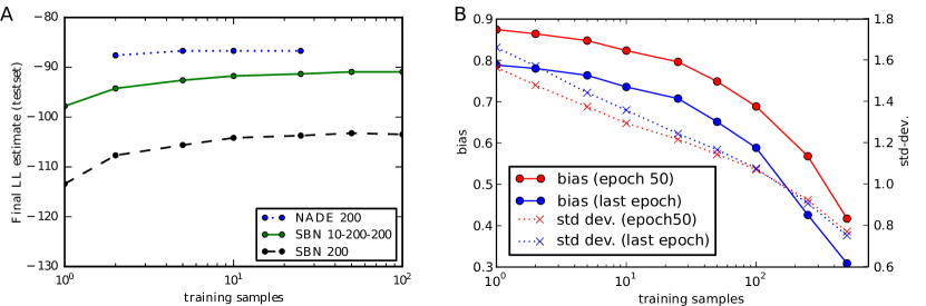
Figure 1: A Final log-likelihood estimate w.r.t. number of samples used during training. B $L_{2}$-norm of the bias and standard deviation of the low-sample estimated $p_{\theta}$ gradient relative to a high-sample (K=5,000) based estimate.

		NVIL	wake-sleep	RWS	RWS
P-model	size			Q-model: SBN	Q-model: NADE
SBN	200	(113.1)	116.3 (120.7)	103.1	95.0
SBN	200-200	(99.8)	106.9 (109.4)	93.4	91.1
SBN	200-200-200	(96.7)	101.3 (104.4)	90.1	88.9
AR-SBN	200				89.2
AR-SBN	200-200				92.8
NADE	200				86.8
NADE	200-200				87.6

Table 1: MNIST results for various architectures and training methods. In the 3rd column we cite the numbers reported by Mnih and Gregor (2014). Values in brackets are variational NLL bounds, values without brackets report NLL estimates (see section 2.2).

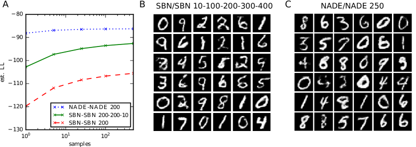
Figure 2: A Final log-likelihood estimate w.r.t. number of test samples used. B Samples from the SBN/SBN 10-200-200 generative model. C Samples from the NADE/NADE 250 generative model. (We show the probabilities from which each pixel is sampled)

Results on binarized MNIST
	NLL	NLL
Method	bound	est.
RWS (SBN/SBN 10-100-200-300-400)		85.48
RWS (NADE/NADE 250)		85.23
RWS (AR-SBN/SBN 500)$\dagger$		84.18
NADE (500 units, [1])		88.35
EoNADE (2hl, 128 orderings, [2])		85.10
DARN (500 units, [3])		84.13
RBM (500 units, CD3, [4])	105.5
RBM (500 units, CD25, [4])	86.34
DBN (500-2000, [5])	86.22	84.55

Results on CalTech 101 Silhouettes
	NLL
Method	est.
RWS (SBN/SBN 10-50-100-300)	113.3
RWS (NADE/NADE 150)	104.3
NADE (500 hidden units)	110.6
RBM (4000 hidden units, [6])	107.8

Table 2: Various RWS trained models in relation to previously published methods: [1] Larochelle and Murray (2011), [2] Murray and Larochelle (2014), [3] Gregor et al. (2014) [4] Salakhutdinov and Murray (2008), [5] Murray and Salakhutdinov (2009), [6] Cho et al. (2013). $\dagger$ Same model as the best performing in [3]: a AR-SBN with deterministic hidden variables between the observed and latent. All RWS NLL estimates on MNIST have confidence intervals of $\approx\pm 0.40$.

We use the MNIST dataset that was binarized according to Murray and Salakhutdinov (2009) and downloaded in binarized form from (Larochelle, 2011). For training we use stochastic gradient decent with momentum ($\beta$=0.95) and set mini-batch size to 25. The experiments in this paragraph were run with learning rates of {0.0003, 0.001, and 0.003}. From these three we always report the experiment with the highest validation log-likelihood. In the majority of our experiments a learning rate of 0.001 gave the best results, even across different layer models (SBN, AR-SBN and NADE). If not noted otherwise, we use $K=5$ samples during training and $K=100,000$ samples to estimate the final log-likelihood on the test set. To disentangle the influence of the different q updating methods we setup $p$ and $q$ networks consisting of three hidden SBN layers with 10, 200 and 200 units (SBN/SBN 10-200-200). After convergence, the model trained updating q during the sleep phase only reached a final estimated log-likelihood of $-93.4$, the model trained with a q-update during the wake phase reached $-92.8$, and the model trained with both wake and sleep phase update reached $-91.9$. As a control we trained a model that does not update $q$ at all. This model reached $-171.4$. We confirmed that combining wake and sleep phase q-updates generally gives the best results by repeating this experiment with various other architectures. For the remainder of this paper we therefore train all models with combined wake and sleep phase q-updates.

Next we investigate the influence of the number of samples used during training. The results are visualized in Fig. 1 A. Although the results depend on the layer-distributions and on the depth and width of the architectures, we generally observe that the final estimated log-likelihood does not improve significantly when using more than 5 samples during training for NADE models, and using more than 25 samples for models with SBN layers. We can quantify the bias and the variance of the gradient estimator (3) using bootstrapping. While training a SBN/SBN 10-200-200 model with $K=100$ training samples, we use $K=5,000$ samples to get a high quality estimate of the gradient for a small but fixed set of 25 datapoints (the size of one mini-batch). By repeatedly resampling smaller sets of $\{1,2,5,\cdots,5000\}$ samples with replacement and by computing the gradient based on these, we get a measure for the bias and the variance of the small sample estimates relative the high quality estimate. These results are visualized in Fig. 1 B. In Fig. 2 A we finally investigate the quality of the log-likelihood estimator (eqn. 1) when applied to the MNIST test set.

Table 1 summarizes how different architectures compare to each other and how RWS compares to related methods for training directed models. We essentially observe that RWS trained models consistently improve over classical wake-sleep, especially for deep architectures. We furthermore observe that using autoregressive layers (AR-SBN or NADE) for the inference network improves the results even when the generative model is composed of factorial SBN layers. Finally, we see that the best performing models with autoregressive layers in $p$ are always shallow with only a single hidden layer. In Table 2 (left) we compare some of our best models to the state-of-the-art results published on MNIST. The deep SBN/SBN 10-100-200-300-400 model was trained for 1000 epochs with $K=5$ training samples and a learning rate of $0.001$. For fine-tuning we run additional 500 epochs with a learning rate decay of $1.005$ and 100 training samples. For comparison we also train the best performing model from the DARN paper (Gregor et al., 2014) with RWS, i.e., a single layer AR-SBN with 500 latent variables and a deterministic layer of hidden variables between the observed and the latents. We essentially obtain the same final testset log-likelihood. For this shallow network we thus do not observe any improvement from using RWS.

4.2 CalTech 101 Silhouettes

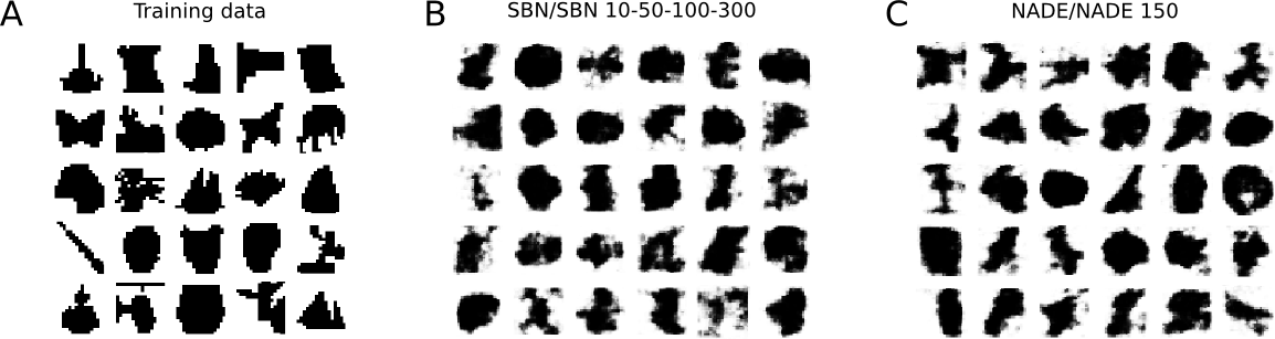
Figure 3: CalTech 101 Silhouettes: A Random selection of training data points. B Random samples from the SBN/SBN 10-50-100-300 generative network. C Random Samples from the NADE-150 generative network. (We show the probabilities from which each pixel is sampled)

We applied reweighted wake-sleep to the $28\times 28$ pixel CalTech 101 Silhouettes dataset. This dataset consists of 4,100 examples in the training set, 2,264 examples in the validation set and 2,307 examples in the test set. We trained various architectures on this dataset using the same hyperparameter as for the MNIST experiments. Table 2 (right) summarizes our results. Note that our best SBN/SBN model is a relatively deep network with 4 hidden layers (300-100-50-10) and reaches a estimated LL of -116.9 on the test set. Our best network, a shallow NADE/NADE-150 network reaches -104.3 and improves over the previous state of the art ($-107.8$, a RBM with 4000 hidden units by Cho et al. (2013)).

5 Conclusions

We introduced a novel training procedure for deep generative models consisting of multiple layers of binary latent variables. It generalizes and improves over the wake-sleep algorithm providing a lower bias and lower variance estimator of the log-likelihood gradient at the price of more samples from the inference network. During training the weighted samples from the inference network decouple the layers such that the learning gradients only propagate within the individual layers. Our experiments demonstrate that a small number of $\approx 5$ samples is typically sufficient to jointly train relatively deep architectures of at least 5 hidden layers without layerwise pretraining and without carefully tuning learning rates. The resulting models produce reasonable samples (by visual inspection) and they approach state-of-the-art performance in terms of log-likelihood on several discrete datasets.

We found that even in the cases when the generative networks contain SBN layers only, better results can be obtained with inference networks composed of more powerful, autoregressive layers. This however comes at the price of reduced computational efficiency on e.g. GPUs as the individual variables $h_{i}\sim q(h|{\mathbf{x}})$ have to be sampled in sequence (even though the theoretical complexity is not significantly worse compared to SBN layers).

We furthermore found that models with autoregressive layers in the generative network $p$ typically produce very good results. But the best ones were always shallow with only a single hidden layer. At this point it is unclear if this is due to optimization problems.

Acknowledgments    We would like to thank Laurent Dinh, Vincent Dumoulin and Li Yao for helpful discussions and the developers of Theano (Bergstra et al., 2010; Bastien et al., 2012) for their powerful software. We furthermore acknowledge CIFAR and Canada Research Chairs for funding and Compute Canada, and Calcul Québec for providing computational resources.

6 Supplement

6.1 Gradients for $p({\mathbf{x}},{\mathbf{h}})$

$$\frac{\partial}{\partial\theta}{\cal L}_{p}(\theta,{\mathbf{x}}\sim{\cal D}) =\frac{\partial}{\partial\theta}\log p_{\theta}({\mathbf{x}})=\frac{1}{p({\mathbf{x}})}\frac{\partial}{\partial\theta}\sum_{{\mathbf{h}}}p({\mathbf{x}},{\mathbf{h}})$$

$$=\frac{1}{p({\mathbf{x}})}\sum_{{\mathbf{h}}}p({\mathbf{x}},{\mathbf{h}})\frac{\partial}{\partial\theta}\log p({\mathbf{x}},{\mathbf{h}})$$

$$=\frac{1}{p({\mathbf{x}})}\sum_{{\mathbf{h}}}q\left({\mathbf{h}}\,|\,{\mathbf{x}}\right)\frac{p({\mathbf{x}},{\mathbf{h}})}{q\left({\mathbf{h}}\,|\,{\mathbf{x}}\right)}\frac{\partial}{\partial\theta}\log p({\mathbf{x}},{\mathbf{h}})$$

$$=\frac{1}{p({\mathbf{x}})}\mathop{{\mathbb{E}}}_{{\mathbf{h}}\sim q\left({\mathbf{h}}\,|\,{\mathbf{x}}\right)}\left[\frac{p({\mathbf{x}},{\mathbf{h}})}{q\left({\mathbf{h}}\,|\,{\mathbf{x}}\right)}\frac{\partial}{\partial\theta}\log p({\mathbf{x}},{\mathbf{h}})\right]$$

$$\simeq\frac{1}{\sum_{k}\omega_{k}}\sum_{k=1}^{K}\omega_{k}\frac{\partial}{\partial\theta}\log p({\mathbf{x}},{\mathbf{h}}^{(k)})$$ (10)

with $$\omega_{k}=\frac{p({\mathbf{x}},{\mathbf{h}}^{(k)})}{q\left({\mathbf{h}}^{(k)}\,|\,{\mathbf{x}}\right)}\;\text{and}\;{\mathbf{h}}^{(k)}\sim q\left({\mathbf{h}}\,|\,{\mathbf{x}}\right)$$

6.2 Gradients for the wake phase q update

$$\frac{\partial}{\partial\phi}{\cal L}_{q}(\phi,{\mathbf{x}}\sim{\cal D}) =\frac{\partial}{\partial\phi}\sum_{{\mathbf{h}}}p({\mathbf{x}},{\mathbf{h}}){\log q_{\phi}({\mathbf{h}}|{\mathbf{x}})}$$

$$=\frac{1}{p({\mathbf{x}})}\mathop{{\mathbb{E}}}_{{\mathbf{h}}\sim q\left({\mathbf{h}}\,|\,{\mathbf{x}}\right)}\left[\frac{p({\mathbf{x}},{\mathbf{h}})}{q\left({\mathbf{h}}\,|\,{\mathbf{x}}\right)}\frac{\partial}{\partial\phi}\log q_{\phi}({\mathbf{h}}|{\mathbf{x}})\right]$$

$$\simeq\frac{1}{\sum_{k}\omega_{k}}\sum_{k=1}^{K}\omega_{k}\frac{\partial}{\partial\phi}\log q_{\phi}({\mathbf{h}}^{(k)}|{\mathbf{x}})$$ (11)

Note that we arrive at the same gradients when we set out to minimize the $KL(p(\cdot|{\mathbf{x}})\parallel q(\cdot|{\mathbf{x}})$ for a given datapoint ${\mathbf{x}}$:

$$\frac{\partial}{\partial\phi}KL(p_{\theta}({\mathbf{h}}|{\mathbf{x}})\parallel q_{\phi}({\mathbf{h}}|{\mathbf{x}})) =\frac{\partial}{\partial\phi}\sum_{{\mathbf{h}}}p_{\theta}({\mathbf{h}}|x)\log\frac{p_{\theta}({\mathbf{h}}|{\mathbf{x}})}{q_{\phi}({\mathbf{h}}|{\mathbf{x}})}$$

$$=-\sum_{{\mathbf{h}}}p_{\theta}({\mathbf{h}}|{\mathbf{x}})\frac{\partial}{\partial\phi}\log q_{\phi}({\mathbf{h}}|{\mathbf{x}})$$

$$\simeq-\frac{1}{\sum_{k}\omega_{k}}\sum_{k=1}^{K}\omega_{k}\frac{\partial}{\partial\phi}\log q_{\phi}({\mathbf{h}}^{(k)}|{\mathbf{x}})$$ (12)

6.3 Additional experimental results

6.3.1 Learning curves for MNIST experiments

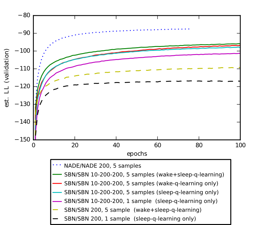
Figure 4: Learning curves for various MNIST experiments.

6.3.2 Bootstrapping based $\log(p(x))$ bias/variance analysis

Here we show the bias/variance analysis from Fig. 1 B (main paper) applied to the estimated $\log(p(x))$ w.r.t. the number of test samples.

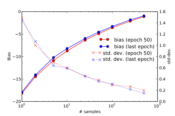
Figure 5: Bias and standard deviation of the low-sample estimated $\log(p(x))$ (bootstrapping with K=5,000 primary samples from a SBN/SBN 10-200-200 network trained on MNIST).

6.3.3 UCI binary datasets

We performed a series of experiments on 8 different binary datasets from the UCI database:

For each dataset we screened a limited hyperparameter space: The learning rate was set to a value in ${0.001,0.003,0.01}$. For SBNs we use $K$=10 training samples and we tried the following architectures: Two hidden layers with 10-50, 10-75, 10-100, 10-150 or 10-200 hidden units and three hidden layers with 5-20-100, 10-50-100, 10-50-150, 10-50-200 or 10-100-300 hidden units. We trained NADE/NADE models with $K$=5 training samples and one hidden layer with 30, 50, 75, 100 or 200 units in it.

Model	ADULT	CONNECT4	DNA	MUSHROOMS	NIPS-0-12	OCR-LETTERS	RCV1	WEB
FVSBN	13.17	12.39	83.64	10.27	276.88	39.30	49.84	29.35
NADE∗	13.19	11.99	84.81	9.81	273.08	27.22	46.66	28.39
EoNADE+	13.19	12.58	82.31	9.68	272.38	27.31	46.12	27.87
DARN3	13.19	11.91	81.04	9.55	274.68	28.17	46.10	28.83
RWS - SBN	13.65	12.68	90.63	9.90	272.54	29.99	46.16	28.18
hidden units	5-20-100	10-50-150	10-150	10-50-150	10-50-150	10-100-300	10-50-200	10-50-300
RWS - NADE	13.16	11.68	84.26	9.71	271.11	26.43	46.09	27.92
hidden units	30	50	100	50	75	100

Table 3: Results on various binary datasets from the UCI repository. The top two rows quote the baseline results from Larochelle & Murray (2011); the third row shows the baseline results taken from Uria, Murray, Larochelle (2014). (NADE^∗: 500 hidden units; EoNADE⁺: 1hl, 16 ord)

References

- Bastien et al. (2012) Bastien, F., Lamblin, P., Pascanu, R., Bergstra, J., Goodfellow, I. J., Bergeron, A., Bouchard, N., and Bengio, Y. (2012). Theano: new features and speed improvements. Deep Learning and Unsupervised Feature Learning NIPS 2012 Workshop.
- Bengio (2009) Bengio, Y. (2009). Learning deep architectures for AI. Now Publishers.
- Bengio and Bengio (2000) Bengio, Y. and Bengio, S. (2000). Modeling high-dimensional discrete data with multi-layer neural networks. In NIPS’99, pages 400–406. MIT Press.
- Bengio et al. (2013) Bengio, Y., Mesnil, G., Dauphin, Y., and Rifai, S. (2013). Better mixing via deep representations. In Proceedings of the 30th International Conference on Machine Learning (ICML’13). ACM.
- Bergstra et al. (2010) Bergstra, J., Breuleux, O., Bastien, F., Lamblin, P., Pascanu, R., Desjardins, G., Turian, J., Warde-Farley, D., and Bengio, Y. (2010). Theano: a CPU and GPU math expression compiler. In Proceedings of the Python for Scientific Computing Conference (SciPy). Oral Presentation.
- Boulanger-Lewandowski et al. (2012) Boulanger-Lewandowski, N., Bengio, Y., and Vincent, P. (2012). Modeling temporal dependencies in high-dimensional sequences: Application to polyphonic music generation and transcription. In ICML’2012.
- Cho et al. (2013) Cho, K., Raiko, T., and Ilin, A. (2013). Enhanced gradient for training restricted boltzmann machines. Neural computation, 25(3), 805–831.
- Dayan and Hinton (1996) Dayan, P. and Hinton, G. E. (1996). Varieties of helmholtz machine. Neural Networks, 9(8), 1385–1403.
- Dayan et al. (1995) Dayan, P., Hinton, G. E., Neal, R. M., and Zemel, R. S. (1995). The Helmholtz machine. Neural computation, 7(5), 889–904.
- Frey (1998) Frey, B. J. (1998). Graphical models for machine learning and digital communication. MIT Press.
- Gregor et al. (2014) Gregor, K., Danihelka, I., Mnih, A., Blundell, C., and Wierstra, D. (2014). Deep autoregressive networks. In Proceedings of the 31st International Conference on Machine Learning.
- Hinton et al. (1995) Hinton, G. E., Dayan, P., Frey, B. J., and Neal, R. M. (1995). The wake-sleep algorithm for unsupervised neural networks. Science, 268, 1558–1161.
- Hinton et al. (2006) Hinton, G. E., Osindero, S., and Teh, Y. (2006). A fast learning algorithm for deep belief nets. Neural Computation, 18, 1527–1554.
- Kingma and Welling (2014) Kingma, D. P. and Welling, M. (2014). Auto-encoding variational bayes. In Proceedings of the International Conference on Learning Representations (ICLR).
- Larochelle (2011) Larochelle, H. (2011). Binarized mnist dataset. http://www.cs.toronto.edu/~larocheh/public/datasets/binarized_mnist/binarized_mnist_[train|valid|test].amat.
- Larochelle and Murray (2011) Larochelle, H. and Murray, I. (2011). The Neural Autoregressive Distribution Estimator. In Proceedings of the Fourteenth International Conference on Artificial Intelligence and Statistics (AISTATS’2011), volume 15 of JMLR: W&CP.
- Mnih and Gregor (2014) Mnih, A. and Gregor, K. (2014). Neural variational inference and learning in belief networks. In Proceedings of the 31st International Conference on Machine Learning (ICML 2014). to appear.
- Murray and Larochelle (2014) Murray, B. U. I. and Larochelle, H. (2014). A deep and tractable density estimator. In ICML’2014.
- Murray and Salakhutdinov (2009) Murray, I. and Salakhutdinov, R. (2009). Evaluating probabilities under high-dimensional latent variable models. In NIPS’08, volume 21, pages 1137–1144.
- Rezende et al. (2014) Rezende, D. J., Mohamed, S., and Wierstra, D. (2014). Stochastic backpropagation and approximate inference in deep generative models. In ICML’2014.
- Salakhutdinov and Murray (2008) Salakhutdinov, R. and Murray, I. (2008). On the quantitative analysis of deep belief networks. In Proceedings of the International Conference on Machine Learning, volume 25.
- Saul et al. (1996) Saul, L. K., Jaakkola, T., and Jordan, M. I. (1996). Mean field theory for sigmoid belief networks. Journal of Artificial Intelligence Research, 4, 61–76.
- Tang and Salakhutdinov (2013) Tang, Y. and Salakhutdinov, R. (2013). Learning stochastic feedforward neural networks. In NIPS’2013.