Deep Epitomic Convolutional Neural Networks
Abstract
Deep convolutional neural networks have recently proven extremely competitive in challenging image recognition tasks. This paper proposes the epitomic convolution as a new building block for deep neural networks. An epitomic convolution layer replaces a pair of consecutive convolution and max-pooling layers found in standard deep convolutional neural networks. The main version of the proposed model uses mini-epitomes in place of filters and computes responses invariant to small translations by epitomic search instead of max-pooling over image positions. The topographic version of the proposed model uses large epitomes to learn filter maps organized in translational topographies. We show that error back-propagation can successfully learn multiple epitomic layers in a supervised fashion. The effectiveness of the proposed method is assessed in image classification tasks on standard benchmarks. Our experiments on Imagenet indicate improved recognition performance compared to standard convolutional neural networks of similar architecture. Our models pre-trained on Imagenet perform excellently on Caltech-101. We also obtain competitive image classification results on the small-image MNIST and CIFAR-10 datasets.
1 Introduction
Deep learning offers a powerful framework for learning increasingly complex representations for visual recognition tasks. The work of Krizhevsky et al. [15] convincingly demonstrated that deep neural networks can be very effective in classifying images in the challenging Imagenet benchmark [5], significantly outperforming computer vision systems built on top of engineered features like SIFT [20]. Their success spurred a lot of interest in the machine learning and computer vision communities. Subsequent work has improved our understanding and has refined certain aspects of this class of models [28]. A number of different studies have further shown that the features learned by deep neural networks are generic and can be successfully employed in a black-box fashion in other datasets or tasks such as image detection [28, 22, 26, 7, 24, 4].
The deep learning models that so far have proven most successful in image recognition tasks are feed-forward convolutional neural networks trained in a supervised fashion to minimize a regularized training set classification error by back-propagation. Their recent success is partly due to the availability of large annotated datasets and fast GPU computing, and partly due to some important methodological developments such as dropout regularization and rectifier linear activations [15]. However, the key building blocks of deep neural networks for images have been around for many years [17]: (1) convolutional multi-layer neural networks with small receptive fields that spatially share parameters within each layer. (2) Gradual abstraction and spatial resolution reduction after each convolutional layer as we ascend the network hierarchy, most effectively via max-pooling [25, 10].
In this work we build a deep neural network around the epitomic representation [12]. The image epitome is a data structure appropriate for learning translation-aware image representations, naturally disentagling appearance and position modeling of visual patterns. In the context of deep learning, an epitomic convolution layer substitutes a pair of consecutive convolution and max-pooling layers typically used in deep convolutional neural networks. In epitomic matching, for each regularly-spaced input data patch in the lower layer we search across filters in the epitomic dictionary for the strongest response. In max-pooling on the other hand, for each filter in the dictionary we search within a window in the lower input data layer for the strongest response. Epitomic matching is thus an input-centered dual alternative to the filter-centered standard max-pooling.
We investigate two main deep epitomic network model variants. Our first variant employs a dictionary of mini-epitomes at each network layer. Each mini-epitome is only slightly larger than the corresponding input data patch, just enough to accomodate for the desired extent of position invariance. For each input data patch, the mini-epitome layer outputs a single value per mini-epitome, which is the maximum response across all filters in the mini-epitome. Our second topographic variant uses just a few large epitomes at each network layer. For each input data patch, the topographic epitome layer outputs multiple values per large epitome, which are the local maximum responses at regularly spaced positions within each topography.
We quantitatively evaluate the proposed model primarily in image classification experiments on the Imagenet ILSVRC-2012 large-scale image classification task. We train the model by error back-propagation to minimize the classification log-loss, similarly to [15]. Our best mini-epitomic variant achieves 13.6% top-5 error on the validation set, which is 0.6% better than a conventional max-pooled convolutional network of comparable structure whose error rate is 14.2%. Note that the error rate of the original model in [15] is 18.2%, using however a smaller network. All these performance numbers refer to classification with a single network. We also find that the proposed epitomic model converges faster, especially when the filters in the dictionary are mean- and contrast-normalized, which is related to [28]. We have found this normalization to also accelerate convergence of standard max-pooled networks. We further show that a deep epitomic network trained on Imagenet can be effectively used as black-box feature extractor for tasks such as Caltech-101 image classification. Finally, we report excellent image classification results on the MNIST and CIFAR-10 benchmarks with smaller deep epitomic networks trained from scratch on these small-image datasets.
Related work
Our model builds on the epitomic image representation [12], which was initially geared towards image and video modeling tasks. Single-level dictionaries of image epitomes learned in an unsupervised fashion for image denoising have been explored in [1, 2]. Recently, single-level mini-epitomes learned by a variant of K-means have been proposed as an alternative to SIFT for image classification [23]. To our knowledge, epitomes have not been studied before in conjunction with deep models or learned to optimize a supervised objective.
The proposed epitomic model is closely related to maxout networks [8]. Similarly to epitomic matching, the response of a maxout layer is the maximum across filter responses. The critical difference is that the epitomic layer is hard-wired to model position invariance, since filters extracted from an epitome share values in their area of overlap. This parameter sharing significantly reduces the number of free parameters that need to be learned. Maxout is typically used in conjunction with max-pooling [8], while epitomes fully substitute for it. Moreover, maxout requires random input perturbations with dropout during model training, otherwise it is prone to creating inactive features. On the contrary, we have found that learning deep epitomic networks does not require dropout in the convolutional layers – similarly to [15], we only use dropout regularization in the fully connected layers of our network.
Other variants of max pooling have been explored before. Stochastic pooling [27] has been proposed in conjunction with supervised learning. Probabilistic pooling [19] and deconvolutional networks [29] have been proposed before in conjunction with unsupervised learning, avoiding the theoretical and practical difficulties associated with building probabilistic models on top of max-pooling. While we do not explore it in this paper, we are also very interested in pursuing unsupervised learning methods appropriate for the deep epitomic representation.
The topographic variant of the proposed epitomic model naturally learns topographic feature maps. Adjacent filters in a single epitome share values in their area of overlap, and thus constitute a hard-wired topographic map. This relates the proposed model to topographic ICA [9] and related models [21, 13, 16], which are typically trained to optimize unsupervised objectives.
2 Deep Epitomic Convolutional Networks
 |
 |
| (a) | (b) |
2.1 Mini-Epitomic deep networks
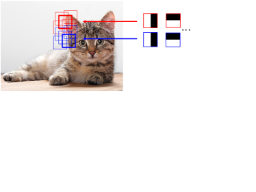
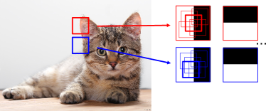
We first describe a single layer of the mini-epitome variant of the proposed model, with reference to Fig. 1. In standard max-pooled convolution, we have a dictionary of filters of spatial size pixels spanning channels, which we represent as real-valued vectors with elements. We apply each of them in a convolutional fashion to every input patch densely extracted from each position in the input layer which also has channels. A reduced resolution output map is produced by computing the maximum response within a small window of displacements around positions in the input map which are pixels apart from each other. The output map of standard max-pooled convolution has spatial resolution reduced by a factor of across each dimension and will consist of channels, one for each of the filters. Specifically:
| (1) |
where points to the input layer position where the maximum is attained.
In the proposed epitomic convolution scheme we replace the filters with larger mini-epitomes of spatial size pixels, where . Each mini-epitome contains filters of size , one for each of the displacements in the epitome. We sparsely extract patches from the input layer on a regular grid with stride pixels. In the proposed epitomic convolution model we reverse the role of filters and input layer patches, computing the maximum response over epitomic positions rather than input layer positions:
| (2) |
where now points to the position in the epitome where the maximum is attained. Since the input position is fixed, we can think of epitomic matching as an input-centered dual alternative to the filter-centered standard max-pooling.
Computing the maximum response over filters rather than image positions resembles the maxout scheme of [8], yet in the proposed model the filters within the epitome are constrained to share values in their area of overlap.
Similarly to max-pooled convolution, the epitomic convolution output map has channels and is subsampled by a factor of across each spatial dimension. Epitomic convolution has the same computational cost as max-pooled convolution. For each output map value, they both require computing inner products followed by finding the maximum response. Epitomic convolution requires times more work per input patch, but this is fully offset by the fact that we extract input patches sparsely with a stride of pixels.
Similarly to standard max-pooling, the main computational primitive is multi-channel convolution with the set of filters in the epitomic dictionary, which we implement as matrix-matrix multiplication and carry out on the GPU, using the cuBLAS library.
To build a deep epitomic model, we stack multiple epitomic convolution layers on top of each other. The output of each layer passes through a rectified linear activation unit and fed as input to the subsequent layer, where is the bias. Similarly to [15], the final two layers of our network for Imagenet image classification are fully connected and are regularized by dropout. We learn the model parameters (epitomic weights and biases for each layer) in a supervised fashion by error back propagation. We present full details of our model architecture and training methodology in the experimental section.
 |
 |
||
| (a) Mini-epitomes | (b) Mini-epitomes + normalization | ||
 |
 |
 |
|
| (c) Max-pooling | (d) Max-pooling + normalization | (e) Topographic + normaliz. | |
2.2 Topographic deep networks
We have also experimented with a topographic variant of the proposed deep epitomic network. For this we use a dictionary with just a few large epitomes of spatial size pixels, with . We retain the local maximum responses over neighborhoods spaced pixels apart in each of the epitomes, thus yielding output values for each of the epitomes in the dictionary. The mini-epitomic variant can be considered as a special case of the topographic one when .
2.3 Optional mean and contrast normalization
Motivated by [28], we have also explored the effect of filter mean and contrast normalization on deep epitomic network training. More specifically, we considered a variant of the model where the epitomic convolution responses are computed as:
| (3) |
where is a mean-normalized version of the filters and is their contrast, with a small positive constant. This normalization requires only a slight modification of the stochastic gradient descent update formula and incurs negligible computational overhead. Note that the contrast normalization explored here is slightly different than the one in [28], who only scale down the filters whenever their contrast exceeds a pre-defined threshold.
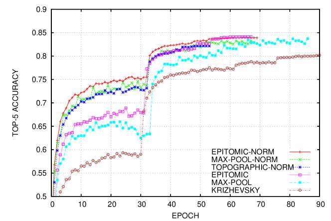
We have found the mean and contrast normalization of Eq. (3) to be crucial for learning the topographic version of the proposed model. We have also found that it significantly accelerates learning of the mini-epitome version of the proposed model, as well as the standard max-pooled convolutional model, without however significantly affecting the final performance of these two model.
3 Image Classification Experiments
3.1 Image classification tasks
We have performed most of our experimental investigation on the Imagenet ILSVRC-2012 dataset [5], focusing on the task of image classification. This dataset contains more than 1.2 million training images, 50,000 validation images, and 100,000 test images. Each image is assigned to one out of 1,000 possible object categories. Performance is evaluated using the top-5 classification error. Such large-scale image datasets have proven so far essential to successfully train big deep neural networks with supervised criteria.
Similarly to other recent works [28, 24, 4], we also evaluate deep epitomic networks trained on Imagenet as a black-box visual feature front-end on the Caltech-101 benchmark [6]. This involves classifying images into one out of 102 possible image classes. We further consider two standard classification benchmarks involving thumbnail-sized images, the MNIST digit [18] and the CIFAR-10 [14], both involving classification into 10 possible classes.
3.2 Network architecture and training methodology
For our Imagenet experiments, we compare the proposed deep mini-epitomic and topographic deep networks with deep convolutional networks employing standard max-pooling. For fair comparison, we use as similar architectures as possible, involving in all cases six convolutional layers, followed by two fully-connected layers and a 1000-way softmax layer. We use rectified linear activation units throughout the network. Similarly to [15], we apply local response normalization (LRN) to the output of the first two convolutional layers and dropout to the output of the two fully-connected layers.
| Layer | 1 | 2 | 3 | 4 | 5 | 6 | 7 | 8 | Out |
|---|---|---|---|---|---|---|---|---|---|
| Type | conv + | conv + | conv | conv | conv | conv + | full + | full + | full |
| lrn + max | lrn + max | max | dropout | dropout | |||||
| Output channels | 96 | 192 | 256 | 384 | 512 | 512 | 4096 | 4096 | 1000 |
| Filter size | 8x8 | 6x6 | 3x3 | 3x3 | 3x3 | 3x3 | - | - | - |
| Input stride | 2x2 | 1x1 | 1x1 | 1x1 | 1x1 | 1x1 | - | - | - |
| Pooling size | 3x3 | 2x2 | - | - | - | 3x3 | - | - | - |
The architecture of our baseline Max-Pool network is specified on Table 1. It employs max-pooling in the convolutional layers 1, 2, and 6. To accelerate computation, it uses an image stride equal to 2 pixels in the first layer. It has a similar structure with the Overfeat model [26], yet significantly fewer neurons in the convolutional layers 2 to 6. Another difference with [26] is the use of LRN, which to our experience facilitates training.
The architecture of the proposed Epitomic network is specified on Table 2. It has exactly the same number of neurons at each layer as the Max-Pool model but it uses mini-epitomes in place of convolution + max pooling at layers 1, 2, and 6. It uses the same filter sizes with the Max-Pool model and the mini-epitome sizes have been selected so as to allow the same extent of translation invariance as the corresponding layers in the baseline model. We use input image stride equal to 4 pixels and further perform epitomic search with stride equal to 2 pixels in the first layer to also accelerate computation.
| Layer | 1 | 2 | 3 | 4 | 5 | 6 | 7 | 8 | Out |
|---|---|---|---|---|---|---|---|---|---|
| Type | epit-conv | epit-conv | conv | conv | conv | epit-conv | full + | full + | full |
| + lrn | + lrn | dropout | dropout | ||||||
| Output channels | 96 | 192 | 256 | 384 | 512 | 512 | 4096 | 4096 | 1000 |
| Epitome size | 12x12 | 8x8 | - | - | - | 5x5 | - | - | - |
| Filter size | 8x8 | 6x6 | 3x3 | 3x3 | 3x3 | 3x3 | - | - | - |
| Input stride | 4x4 | 3x3 | 1x1 | 1x1 | 1x1 | 3x3 | - | - | - |
| Epitome stride | 2x2 | 1x1 | - | - | - | 1x1 | - | - | - |
The architecture of our second proposed Topographic network is specified on Table 3. It uses four epitomes at layers 1, 2 and eight epitomes at layer 6 to learn topographic feature maps. It uses the same filter sizes as the previous two models and the epitome sizes have been selected so as each layer produces roughly the same number of output channels when allowing the same extent of translation invariance as the corresponding layers in the other two models.
| Layer | 1 | 2 | 3 | 4 | 5 | 6 | 7 | 8 | Out |
|---|---|---|---|---|---|---|---|---|---|
| Type | epit-conv | epit-conv | conv | conv | conv | epit-conv | full + | full + | full |
| + lrn | + lrn | dropout | dropout | ||||||
| Output channels | 4x25 | 4x49 | 256 | 384 | 512 | 8x64 | 4096 | 4096 | 1000 |
| Epitome size | 36x36 | 26x26 | - | - | - | 26x26 | - | - | - |
| Filter size | 8x8 | 6x6 | 3x3 | 3x3 | 3x3 | 3x3 | - | - | - |
| Input stride | 4x4 | 3x3 | 1x1 | 1x1 | 1x1 | 3x3 | - | - | - |
| Epitome stride | 2x2 | 1x1 | - | - | - | 1x1 | - | - | - |
| Epit. pool size | 3x3 | 3x3 | - | - | - | 3x3 | - | - | - |
We have also tried variants of the three models above where we activate the mean and contrast normalization scheme of Section 2.3 in layers 1, 2, and 6 of the network.
We followed the methodology of [15] in training our models. We used stochastic gradient ascent with learning rate initialized to 0.01 and decreased by a factor of 10 each time the validation error stopped improving. We used momentum equal to 0.9 and mini-batches of 128 images. The weight decay factor was equal to . Importantly, weight decay needs to be turned off for the layers that use mean and contrast normalization. Training each of the three models takes two weeks using a single NVIDIA Titan GPU. Similarly to [4], we resized the training images to have small dimension equal to 256 pixels while preserving their aspect ratio and not cropping their large dimension. We also subtracted for each image pixel the global mean RGB color values computed over the whole Imagenet training set. During training, we presented the networks with crops randomly sampled from the resized image area, flipped left-to-right with probability 0.5, also injecting global color noise exactly as in [15]. During evaluation, we presented the networks with 10 regularly sampled image crops (center + 4 corners, as well as their left-to-right flipped versions).
3.3 Weight visualization
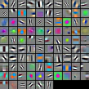
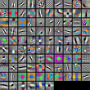
We visualize in Figure 2 the layer weights at the first layer of the networks above. The networks learn receptive fields sensitive to edge, blob, texture, and color patterns.
3.4 Classification results
We report at Table 4 our results on the Imagenet ILSVRC-2012 benchmark, also including results previously reported in the literature [15, 28, 26]. These all refer to the top-5 error on the validation set and are obtained with a single network. Our best result at 13.6% with the proposed Epitomic-Norm network is 0.6% better than the baseline Max-Pool result at 14.2% error. Our Topographic-Norm network scores less well, yielding 15.4% error rate, which however is still better than [15, 28]. Mean and contrast normalization had little effect on final performance for the Max-Pool and Epitomic models, but we found it essential for learning the Topographic model. The improved performance that we got with the Max-Pool baseline network compared to Overfeat [26] is most likely due to our use of LRN and aspect ratio preserving image resizing. When preparing this manuscript, we became aware of the work of [4] that reports an even lower 13.1% error rate with a max-pooled network, using however significantly more neurons than we do in the convolutional layers 2 to 5.
| Model | Krizhevsky | Zeiler-Fergus | Overfeat | Max-Pool | Max-Pool | Epitomic | Epitomic | Topographic |
| [15] | [28] | [26] | + norm | + norm | + norm | |||
| Top-5 Error | 18.2% | 16.0% | 14.7% | 14.2% | 14.4% | 13.7% | 13.6% | 15.4% |
We next assess the quality of the proposed model trained on Imagenet as black-box feature extractor for Caltech-101 image classification. For this purpose, we used the 4096-dimensional output of the last fully-connected layer, without doing any fine-tuning of the network weights for the new task. We trained a 102-way SVM classifier using libsvm [3] and the default regularization parameter. For this experiment we just resized the Caltech-101 images to size without preserving their aspect ratio and computed a single feature vector per image. We normalized the feature vector to have unit length before feeding it into the SVM. We report at Table 5 the mean classification accuracy obtained with the different networks. The proposed Epitomic model performs at 87.8%, 0.5% better than the baseline Max-Pool model.
| Model | Zeiler-Fergus | Max-Pool | Max-Pool | Epitomic | Epitomic | Topographic |
|---|---|---|---|---|---|---|
| [28] | + norm | + norm | + norm | |||
| Mean Accuracy | 86.5% | 87.3% | 85.3% | 87.8% | 87.4% | 85.8% |
We have also performed experiments with the epitomic model on classifying small images on the MNIST and CIFAR-10 datasets. For these tasks we have trained much smaller networks from scratch, using three epitomic convolutional layers, followed by one fully-connected layer and the final softmax classification layer. Because of the small training set sizes, we have found it beneficial to also employ dropout regularization in the epitomic convolution layers. At Table 6 we report the classification error rates we obtained. Our results are comparable to maxout [8], which achieves state-of-art results on these tasks.
|
|
||||||||||||
|---|---|---|---|---|---|---|---|---|---|---|---|---|---|
| (a) MNIST | (b) CIFAR-10 |
3.5 Mean-contrast normalization and convergence speed
We comment on the learning speed and convergence properties of the different models we experimented with on Imagenet. We show in Figure 3 how the top-5 validation error improves as learning progresses for the different models we tested, with or without mean+contrast normalization. For reference, we also include a corresponding plot we re-produced for the original model of Krizhevsky et al. [15]. We observe that mean+contrast normalization significantly accelerates convergence of both epitomic and max-pooled models, without however significantly influencing the final model quality. The epitomic models exhibit somewhat improved convergence behavior during learning compared to the max-pooled baselines whose performance fluctuates more.
4 Conclusions
In this paper we have explored the potential of the epitomic representation as a building block for deep neural networks. We have shown that an epitomic layer can successfully substitute a pair of consecutive convolution and max-pooling layers. We have proposed two deep epitomic variants, one featuring mini-epitomes that empirically performs best in image classification, and one featuring large epitomes and learns topographically organized feature maps. We have shown that the proposed epitomic model performs around 0.5% better than the max-pooled baseline on the challenging Imagenet benchmark and other image classification tasks.
In future work, we are very interested in developing methods for unsupervised or semi-supervised training of deep epitomic models, exploiting the fact that the epitomic representation is more amenable than max-pooling for incorporating image reconstruction objectives.
Reproducibility
We implemented the proposed methods by extending the excellent Caffe software framework [11]. When this work gets published we will publicly share our source code and configuration files with exact parameters fully reproducing the results reported in this paper.
Acknowledgments
We gratefully acknowledge the support of NVIDIA Corporation with the donation of GPUs used for this research.
References
- [1] M. Aharon and M. Elad. Sparse and redundant modeling of image content using an image-signature-dictionary. SIAM J. Imaging Sci., 1(3):228–247, 2008.
- [2] L. Benoît, J. Mairal, F. Bach, and J. Ponce. Sparse image representation with epitomes. In Proc. CVPR, pages 2913–2920, 2011.
- [3] C.-C. Chang and C.-J. Lin. LIBSVM: a library for support vector machines. ACM Trans. on Intel. Systems and Tech., 2(3), 2011.
- [4] K. Chatfield, K. Simonyan, A. Vedaldi, and A. Zisserman. Return of the devil in the details: Delving deep into convolutional nets. arXiv, 2014.
- [5] J. Deng, W. Dong, R. Socher, L. Li-Jia, K. Li, and L. Fei-Fei. Imagenet: A large-scale hierarchical image database. In Proc. CVPR, 2009.
- [6] L. Fei-Fei, R. Fergus, and P. Perona. Learning generative visual models from few training examples: An incremental Bayesian approach tested on 101 object categories. In Proc. CVPR Workshop, 2004.
- [7] R. Girshick, J. Donahue, T. Darrell, and J. Malik. Rich feature hierarchies for accurate object detection and semantic segmentation. In Proc. CVPR, 2014.
- [8] I. Goodfellow, D. Warde-Farley, M. Mirza, A. Courville, and Y. Bengio. Maxout networks. In Proc. ICML, 2013.
- [9] A. Hyvärinen, P. Hoyer, and M. Inki. Topographic independent component analysis. Neur. Comp., 13(7):1527–1558, 2001.
- [10] K. Jarrett, K. Kavukcuoglu, M. Ranzato, and Y. LeCun. What is the best multi-stage architecture for object recognition? In Proc. ICCV, pages 2146–2153, 2009.
- [11] Y. Jia. Caffe: An open source convolutional architecture for fast feature embedding. http://caffe.berkeleyvision.org/, 2013.
- [12] N. Jojic, B. Frey, and A. Kannan. Epitomic analysis of appearance and shape. In Proc. ICCV, pages 34–41, 2003.
- [13] K. Kavukcuoglu, M. Ranzato, R. Fergus, and Y. LeCun. Learning invariant features through topographic filter maps. In Proc. CVPR, 2009.
- [14] A. Krizhevsky. Learning multiple layers of features from tiny images. Technical report, 2009.
- [15] A. Krizhevsky, I. Sutskever, and G. Hinton. ImageNet classification with deep convolutional neural networks. In Proc. NIPS, 2013.
- [16] Q. Le, M. Ranzato, R. Monga, M. Devin, G. Corrado, K. Chen, J. Dean, and A. Ng. Building high-level features using large scale unsupervised learning. In Proc. ICML, 2012.
- [17] Y. LeCun, L. Bottou, Y. Bengio, and P. Haffner. Gradient-based learning applied to document recognition. Proc. IEEE, 86(11):2278–2324, 1998.
- [18] Y. LeCun and C. Cortes. The MNIST database of handwritten digits, 1998.
- [19] H. Lee, R. Grosse, R. Ranganath, and A. Y. Ng. Convolutional deep belief networks for scalable unsupervised learning of hierarchical representations. In Proc. ICML, 2009.
- [20] D. Lowe. Distinctive image features from scale-invariant keypoints. IJCV, 60(2):91–110, 2004.
- [21] S. Osindero, M. Welling, and G. Hinton. Topographic product models applied to natural scene statistics. Neur. Comp., 18:381–414, 2006.
- [22] W. Ouyang and X. Wang. Joint deep learning for pedestrian detection. In Proc. ICCV, 2013.
- [23] G. Papandreou, L.-C. Chen, and A. Yuille. Modeling image patches with a generic dictionary of mini-epitomes. In Proc. CVPR, 2014.
- [24] A. Razavian, H. Azizpour, J. Sullivan, and S. Carlsson. CNN features off-the-shelf: An astounding baseline for recognition. In Proc. CVPR Workshop, 2014.
- [25] M. Riesenhuber and T. Poggio. Hierarchical models of object recognition in cortex. Nature neuroscience, 2(11):1019–1025, 1999.
- [26] P. Sermanet, D. Eigen, X. Zhang, M. Mathieu, R. Fergus, and Y. LeCun. Overfeat: Integrated recognition, localization and detection using convolutional networks. 2014.
- [27] M. Zeiler and R. Fergus. Stochastic pooling for regularization of deep convolutional neural networks. 2013.
- [28] M. Zeiler and R. Fergus. Visualizing and understanding convolutional networks. arXiv, 2013.
- [29] M. Zeiler, D. Krishnan, G. Taylor, and R. Fergus. Deconvolutional networks. In Proc. CVPR, 2010.