[1406.2731] 1 Introduction

Calculus from a

Statistics Perspective

SAMUEL S.P. SHEN, DOV ZAZKIS, KIMBERLY LEUNG, and

CHRIS RASMUSSEN

Department of Mathematics and Statistics, San Diego State University,

San Diego, CA 92182, USA.

Email: sam.shen@sdsu.edu

Abstract This paper provides an approach to establishing the calculus method from the concept of mean, i.e., average. This approach is from a statistics perspective and can help calculus learners understand calculus ideas and analyze a function defined by data or sampling values from a given function, rather than an explicit mathematical formula. The basics of this approach are two averages: arithmetic mean and graphic mean. The arithmetic mean is used to define integral. Area is used to interpret the meaning of an integral. Antiderivative is introduced from integral, and derivative-antiderivative pair is introduced as a mathematical operation entity. The graphic mean is an average speed in an interval and is used to interpret the meaning of a derivative.

1 Introduction

How can one use elementary statistics method to help explain ideas of calculus? The purpose of this paper is to provide an approach to developing calculus methods from a statistics perspective. Our approach is motivated in part by mathematical modeling (ref. [5]), and can be helpful for enhancing the link between elementary statistics courses and calculus courses. The link is developed from statistics to calculus and is different from the traditional connection from calculus to statistics.

A mathematical function $y=f(x)$ can be represented in four ways (see p11 of Stewart (2008) [10]): (i) a description in words or text, (ii) a table of at least two columns of data, (iii) a graph in the x-y coordinates plane, and (iv) an explicit mathematical formula. Conventional calculus textbooks (e.g., [1, 10]) almost exclusively deal with Case (iv): functions defined by explicit formulas. The graphic representations (i.e., Case (iii)) are dealt with as a supporting tool for the function formula. Case (ii), data-represented functions, is usually considered the category of statistics, which analyzes data and makes inferences for the data’s implications. Hence, most calculus textbooks do not deal with this case even in the modern era of computers. However, the rapid development of data-based information in our practical life requires us to broaden the traditional statistics methods, including interconnections between statistics and calculus. Today’s speed and availability of personal computers and smart phones make it possible to take new and innovative approaches to calculus for functions represented in any of the four ways. This paper will develop the calculus ideas from statistics perspective. We will build the calculus concept for the function of Case (ii) and make the concept applicable to the functions of all the four cases. We use two types of averages: arithmetic mean and graphic mean. The arithmetic mean and law of large numbers (LLN) are used to define an integral, and graphic mean is to define a derivative.

We do not intend to use this approach to replace the conventional way of teaching calculus. Instead, our proposed approach may be used as supplemental material in today’s classrooms of conventional calculus and hence provides a new perspective for explaining calculus ideas to students. Further, we do not claim that this approach is superior to other approaches to calculus. Every approach to calculus has its own disadvantages. Ours is not an exception.

Two co-authors have experimented the new approach in two different courses. Shen used it in Calculus I for engineering and physical sciences in the Fall 2011, where he spent two hours altogether at the beginning of the course on the new approach in a class of 120 students. After the two hours, he asked his students to explain the concept of integral to their grandmother. Zakis taught this material to four students in the summer of 2011 in the third mathematics course in a sequence of four courses for prospective elementary school teachers. This third mathematics course’s main contents are on probability and statistics. He made an educational pedagogy study from this course and spent over four hours on this approach with emphasis on understanding the concept of integrals (Zazkis et al. (2014) [ref. 12]). Therefore, our modest goals of the calculus from statistics perspective are (a) to provide a set of supplemental materials to explain the the concept of calculus from a non-traditional perspective, and (b) to provide research opportunities for mathematics education.

To simplify the description of our approach to the integral and derivative concept, we limit our functions to those that are continuous and smooth with positive domain and positive range, when discussing the Case (iv) function $y=f(x)$ . These limits do not affect the rigor of the mathematics developed here and can be easily removed when a more sophisticated mathematics of calculus is introduced.

2 Arithmetic mean, sampling, and average of a function

For a given location on Earth, its temperature’s variation with respect to time forms a functional relationship. Consider the arithmetic mean for the annual surface air temperature (SAT) data (in units [^∘C]) data from 1951-2010 at Fredericksburg (38.32^∘N, 77.45^∘W), which is 80 kilometers southwest of Washington DC, United States (See Table 1). The data pairs $(x_{i},f_{i})(i=1,2,\cdots,n)$ represent the tabular form of a function (the Case (ii) function) with $x_{i}$ for time and $f_{i}$ for temperature, and $n$ is 60 for this case. Arithmetic mean is defined as

\bar{f}=\frac{\sum_{i=1}^{n}f_{i}}{n}.

(1)

For the SAT data in Table 1, the mean is 13.2[^∘C].

Table 1. Annual mean SAT at Fredericksburg from 1951- 2010

Annual mean surface air temperature at Fredericksburg (38.32^∘N, 77.45^∘W)
Virginia, United States. The temperature units are [^∘C]. The data are from
the U.S. Historical Climatology Network.
http://www.ncdc.noaa.gov/oa/climate/research/ushcn/
1951	13.1	1961	12.9	1971	13.2	1981	12.5	1991	14.3	2001	13.7
1952	13.4	1962	12.3	1972	12.8	1982	12.7	1992	12.5	2002	14.3
1953	14.4	1963	12.4	1973	13.7	1983	12.8	1993	13.2	2003	13.0
1954	13.7	1964	13.2	1974	13.3	1984	13.0	1994	13.2	2004	13.6
1955	12.6	1965	12.7	1975	13.0	1985	13.6	1995	13.2	2005	13.7
1956	13.1	1966	12.4	1976	12.6	1986	13.4	1996	12.6	2006	14.2
1957	13.3	1967	12.3	1977	13.1	1987	13.4	1997	13.0	2007	14.1
1958	12.1	1968	12.8	1978	12.3	1988	12.6	1998	14.7	2008	13.7
1959	13.6	1969	12.5	1979	12.5	1989	12.9	1999	13.9	2009	13.2
1960	12.6	1970	13.1	1980	12.7	1990	14.3	2000	13.0	2010	14.2

Next we explore the data that are samples from the Case (iv) functional values. The samples of independent and dependent variables are $(x_{i},y_{i}),i=1.2.\cdots,n$ , where the Case (iv) function is denoted by $y=f(x)$ . The sampling of $x$ is usually done in three ways.

(i)

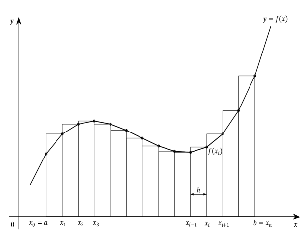
Uniform sampling: The distance between each pair of neighborhood samples is the same, i.e., $h=x_{i}-x_{i-1}$ is the same for each $i$ . The sample points can be determined by $x_{i}=x_{i-1}+h,i=1,2,\cdots,n$ . An example is the SAT sampling in Table 1 whose $h$ is one year. Another example is a uniform sampling of a function shown in Figure 1.
(ii)

Random sampling: Random sampling is, by name, a probability process and can be determined by a predefined way using a statistics software. Many software tools for generating random numbers are available in pubic domain for free, such as WolframAlpha: www.wolframalpha.com. The command RandomReal[{0,2},10] yields 10 random real numbers in the interval $[0,2]$ . A trial of this command is
{1.25685, 1.02584, 1.26752, 0.813785, 0.224482, 0.905491, 1.73265, 1.44104, 1.95108, 0.926807}
Of course, each trial yields a different random result.
(iii)

Convenience sampling: This sampling may be neither as evenly spaced as the uniform sampling nor completely random, but the samples are taken from convenient and practical locations, such as the location of weather stations, which could be neither at the top of Himalayas nor over the midst of Pacific. Thus, convenient sampling is often encountered in practice, such as the data from geology, meteorology, hydrology, agriculture and forestry, but suffers possible drawbacks of bias and incompletion. When given a Case (iv) function, this sampling is unnecessary, but for a function of the other three cases in practical applications, this sampling is essential to describe a function for applications.

Refer to caption — Figure 1: Uniform sampling for a function $y=f(x)$ in $[a,b]$ . The area under the curve is approximated by the sum of the narrow rectangular strips

Let us explore two examples of calculating arithmetic means of sample data from a function: $y=x$ and $y=x^{2}$ .

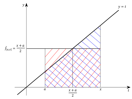
From our intuition or assisted by a figure (see Figure 2 with $a=0$ ), we can infer that the mean of the function $y=x$ in $[0,1]$ is $1/2$ . This result can be simulated by different sampling methods.

(a)

Uniform sampling: We use a sample of size 100 with the first sample at $x=0.01$ and last sample at $x=1$ . These 100 points divide the interval $[0,1]$ into 100 equal sub-intervals of length $1/100$ :

x_{1}=0.01,x_{2}=0.02,\cdots,x_{i}=\frac{i}{100},\cdots,x_{100}=1.

y_{i}=x_{i},i=1,2,\cdots,100

The arithmetic mean of data $y_{i},i=0,1,\cdots,100$ is equal to

\hat{\bar{y}}=\frac{\sum_{i=1}^{100}y_{i}}{100}=\frac{\sum_{i=1}^{100}(i/100)}{100}=\frac{\sum_{i=1}^{100}i}{100\times 100}=0.505,

(2)

which is very close to the exact average value 0.5.

(b)

Random sampling: Random sampling usually does not sample the end points. Our 100 samples are at the internal points of $[0,1]$ , i.e., over $(0,1)$ . WolframAlpha command RandomReal[{0,1},100] generates 100 random numbers whose mean is $0.5312$ , which is close to the exact result $0.5$ . Again, the result $0.5312$ is different each time the command is implemented due to the random nature of the RandomReal generator. It is intuitive that larger samples should be likely to lead to more accurate approximation. When using 1000 samples, a result is $0.4981$ , which is very close to $0.5$ .

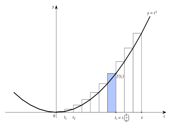
Next we consider $y=x^{2}$ in $[0,1]$ (see Figure 3). The uniform sampling of using 100 points as above yields the following:

\hat{\bar{y}}=\frac{\sum_{i=1}^{100}y_{i}^{2}}{100}=\frac{\sum_{i=1}^{100}(i/100)^{2}}{100}=\frac{\sum_{i=0}^{100}i^{2}}{100^{2}\times 100}=\frac{100\times(100+1)(2\times 100+1)/6}{100^{2}\times 100}=\frac{101\times 201}{6\times 100^{2}}=.33835

The random sampling with WolframAlpha uses a command RandomReal[{0,1},10]2̂ to generate the data, and the text result can be copied and used to calculate the mean by using WolframAlpha. A result is $0.36726$ . The accurate mean value should be $0.33333$ , which can be computed from $n$ samples when $n$ is very large.

WolframAlpha has limited statistical computing power. The open source statistics software R and the commonly used MS Excel have more statistical computing power and can be used for practical applications and research. An Excel calculation of the sample mean for $y=x^{2}$ in $[0,1]$ for different number of samples is given in Table 2, which indicates that, in general, the accuracy of the mean improves as the sample size $n$ increases. As a matter of fact, the improvement of the accuracy can be quantified by the error $\sigma/\sqrt{n}$ where $\sigma$ is the standard deviation of the population being sampled. This is a result of the Central Limit Theorem (CLT) in statistics (see a basic statistics text, e.g., [4, 11] ). The CLT states that the mean of samples with sufficiently large sample size is normally distributed. CLT further asserts that (i) the expected value of the sample mean is the same as the population mean, and (ii) the variance of the sample mean is $(1/n)$ th of the population variance. These two assertions are widely assumed in practical statistical applications and computer calculations, such as Monte Carlo simulations. This is normal distribution result can be intuitive to students and may be accepted as an axiom. However, instructor does not need to teach the CLT to students in this first introduction of calculus from statistics perspective. This is like the case that the first introduction of conventional calculus does not need to prove the existence of a limit from the rigorous $\delta-\epsilon$ argument.

Table 2. Convergence of the sample mean as the sample size increases.

Sample Size n	10	100	1,000	10,000	100,000	1,000,000
Uniform Sampling	0.3850	0.3384	0.3338	0.3334	0.3333	0.3333
Random Sampling
Trial 1	0.4350	0.3505	0.3463	0.3344	0.3315	0.3332
Trial 2	0.3560	0.3058	0.3284	0.3325	0.3331	0.3332
Trial 3	0.4640	0.3518	0.3355	0.3317	0.3357	0.3332
Average	0.4183	0.3360	0.3367	0.3329	0.3335	0.3332

Let $\hat{\bar{f}}[n]$ denote the mean from $n$ samples. Then, it is almost always true that $\hat{\bar{f}}[n]$ approaches the true mean of the function as $n$ increases. This convergence has a probability equal to one. The probability for this to be false is zero. This intuitive conclusion is the strong LLN (see [10]), which asserts that the event of the following limit being true has a probability equal to one:

\lim_{n\to\infty}\hat{\bar{f}}[n]=\bar{f}.

(3)

Here $\bar{f}$ is the limit of the sequence $\{\hat{\bar{f}}[1],\hat{\bar{f}}[2],\hat{\bar{f}}[3],\cdots\}$ , or simply $\{\hat{\bar{f}}[n]\}$ .

For example, when $x^{2}$ is uniformly sampled by $n$ points over $[0,1]$ , the mean is

\hat{\bar{f}}[n]=\frac{\sum_{i=1}^{n}(i/n)^{2}}{n}=\frac{\sum_{i=0}^{n}i^{2}}{n\times n^{2}}=\frac{n(n+1)(2n+1)/6}{n^{3}}=\frac{n+1}{n}\times\frac{2n+1}{6n}.

As $n\to\infty$ , the first factor goes to 1 and the second to 2/6=1/3. Thus, the above mean approaches $1/3\approx 0.33333333$ as $n\to\infty$ .

The above leads to the definition of average of a function $y=f(x)$ in an interval $[a,b]$

\bar{f}=\lim_{n\to\infty}\frac{\sum_{i=1}^{n}f(x_{i})}{n},

(4)

where $\{x_{i}\}_{i=1}^{n}$ are sampled from $[a,b]$ by uniform sampling, random sampling, and possibly convenience sampling. We also call $\bar{f}$ arithmetic mean, or just mean, of the function $y=f(x)$ .

3 Definition of integral, antiderivative, and DA pair

Definition of integral: If $\bar{f}$ is the average of the function $f(x)$ over the interval $[a,b]$ , then $(b-a)\times\bar{f}$ is defined as the integral of $f(x)$ over $[a,b]$ , denoted by

I[f,a,b]=(b-a)\bar{f}

(5)

This serves as the definition of the definite integral in conventional calculus. Since we will not introduce the concept of indefinite integral, we thus treat ”integral” here as the ”definite integral.”

From the examples of mean in the above section, we can calculate the following integrals:

I[x,0,1]=(1-0)\times(1/2)=1/2,

and

I[x^{2},0,1]=(1-0)\times(1/3)=1/3.

Then, what is the graphic meaning of integral from the above definition of integral? We use uniform sampling to make an interpretation. Since $\hat{\bar{f}}[n]\approx\bar{f}$ , we have

I[f,a,b]\approx(b-a)\hat{\bar{f}}[n]=(b-a)\frac{\sum_{i=1}^{n}f_{i}}{n}=\sum_{i=1}^{n}\frac{b-a}{n}f_{i}.

Here $f_{i}=f(x_{i})$ is the sample value of the function at the sampling location $x_{i}$ (see Figure 1). Since this is uniform sampling, $x_{i+1}-x_{i}=h=(b-a)/n$ . Thus, each term in the above sum

\frac{b-a}{n}f_{i}

is the area of a rectangular strip with base $h=(b-a)/n$ and height $f_{i}$ , as shown in Figure 1. Thus, $(b-a)\hat{\bar{f}}[n]$ is the area of under the echelon, formed by $n$ rectangular strips whose heights are determined by the function values from a uniform sampling $f(x_{i})=f(ih),i=1,2,\cdots,n$ . This sum approaches the true area, denoted by $S$ , of the region under the curve $y=f(x)$ in [ $a,b]$ . The ever improving approximation as $n\to\infty$ is a process of limit and is denoted by

\lim_{n\to\infty}(b-a)\hat{\bar{f}}[n]=S=I[f,a,b].

(6)

Dividing both sides by $b-a$ leads to the limit of $\hat{\bar{f}}[n]$ as $n\to\infty$

\lim_{n\to\infty}\hat{\bar{f}}[n]=\bar{f}.

(7)

As mentioned earlier, the existence of this limit is guaranteed by LLN, and the probability for this limit to fail is zero.

Therefore, the geometric meaning of the integral $I[f,a,b]$ is the area of the region bounded by $y=f(x)$ , $y=0$ , $x=a$ and $x=b$ .

Now following Shen and Lin (2014)[ref. [9]), we can define antiderivative and introduce a concept called derivative-antiderivative (DA) pair. We define the integral $I[f,a,x]$ as antiderivative of $f(x)$ and is denoted by $F(x)$ , where $a$ is an arbitrary constant and $x$ is regarded as a variable. We also call $f(x)$ the derivative of $F(x)$ and is denoted by $F^{\prime}(x)=f(x)$ . Because $x$ is regarded as a variable, antiderivative $F(x)$ is a function. The function pair $(f(x),F(x))$ is called a DA pair.

From the geometric meaning of integral, $F(x)=I[f,0,x]$ is the area of the region bounded by $y=f(t)$ , $y=0$ , $t=0$ and $t=x$ over the $t-y$ plane (see Figure 3).

Example 1. Evaluate the antiderivative of $f(x)=1$ .

The area of the rectangle bounded $y=1$ , $y=0$ , $t=0$ and $t=x$ over the $t-y$ plane is $x$ . Thus, $F(x)=x$ , and $(1,x)$ is a DA pair.

Example 2. Evaluate the antiderivative of $f(x)=x$ .

The area of the triangle bounded $y=t$ , $y=0$ , $t=0$ and $t=x$ over the $t-y$ plane is $x^{2}/2$ (See Figure 2). Thus, $F(x)=x^{2}/2$ , and $(x,x^{2}/2)$ is a DA pair, i.e., $(x^{2}/2)^{\prime}=x$ and $I[t,0,x]=x^{2}/2$ .

Example 3. Evaluate the antiderivative of $f(x)=x^{2}$ .

This is a problem of calculating the area of a curved triangle (See Figure 3). We can use the uniform sampling as we have done above for $y=t^{2}$ in the interval $[0,1]$ , but now for the interval $[0,x]$ .

\hat{\bar{f}}[n]=\frac{\sum_{i=1}^{n}(xi/n)^{2}}{n}=x^{2}\frac{\sum_{i=0}^{n}i^{2}}{n\times n^{2}}=x^{2}\frac{n(n+1)(2n+1)/6}{n^{3}}=x^{2}\frac{n+1}{n}\times\frac{2n+1}{6n}.

This mean approaches $x^{2}/3$ as $n\to\infty$ . Hence,

F(x)=(x-0)\times x^{2}/3=x^{3}/3.

We thus have a DA pair $(x^{2},x^{3}/3)$ , i.e., $(x^{3}/3)^{\prime}=x^{2}$ and $I[t^{2},0,x]=x^{3}/3$ .

It is tedious to find an antiderivative by definition as shown above. Fortunately, many free software packages, such as WolframAlpha, are now available over the internet. For example, in the pop up box from WolframAlpha, type integral x4̂. Press the enter key. The WolframAlpha returns the antiderivative $x^{5}/5$ . So $(x^{4},x^{5}/5)$ is a DA pair. In the same way, WolframAlpha can generate the following DA pairs.

(i)

Power function: $(x^{n},x^{n+1}/(n+1))$ .
(ii)

Exponential function: $(e^{x},e^{x})$ .
(iii)

Natural logarithmic function: $(\frac{1}{x},\ln x)$ .
(iv)

Sine function: $(\cos x,\sin x)$ .
(v)

Cosine function: $(-\sin x,\cos x)$ .
(vi)

Tangent function: $(\sec^{2}x,\tan x)$ .

One can also use www.wolframalpha.com to find derivatives. For example, in the pop up box, type derivative x5̂/5 and press enter. It returns $x^{4}$ . This verifies that $(x^{5}/5)^{\prime}=x^{4}$ .

4 Calculation of $I[f,a,b]$

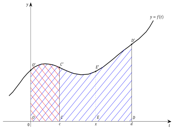
We can use antiderivative to calculate an integral (again following the DA pair idea of Shen and Lin (2014) (ref. 9]). From the area meaning of an integral (see Figure 4), we have the following formula:

I[f,c,d]=F(d)-F(c).

(8)

This is also denoted by $I[f,c,d]=F(x)|^{d}_{c}$ . Namely, the area of the region bounded by $y=f(x)$ , $y=0$ , $x=c$ , and $x=d$ is equal to the difference of the area bounded by $y=f(x)$ , $y=0$ , $x=a$ , and $x=d$ minus the area bounded by $y=f(x)$ , $y=0$ , $x=a$ , and $x=c$ . This is shown in Figure 4: $I[f,c,d]$ is the area CDD^′C^′, equal to area ODD^′O^′minus area OCC^′O^′.

In traditional calculus, this way of calculating an integral is called Part II of the Fundamental Theorem of Calculus (FTC), and the DA pair is called Part I of FTC (e.g., Stewart (2008) [10]).

Example 4. Evaluate $I[x^{2},0,1]$ .

Since $F(x)=I[x^{2}]=x^{3}/3$ , $I[x^{2},0,1]=x^{3}/3|_{0}^{1}=1^{3}/3-0^{3}/3=1/3.$

Example 5. Evaluate $I[sin^{2}(x),0,\pi]$ .

In www.wolframalpha.com, the command integrate sin2̂ x yields $F(x)=(1/2)(x-\sin x\cos x)$ . Thus,

I[\sin^{2}x,0,\pi]=(1/2)(x-\sin x\cos x)|^{\pi}_{0}=(1/2)(\pi-\sin\pi\cos\pi)-(1/2)(0-\sin 0\cos 0)=\pi/2.

One can also use www.wolframalpha.com to calculate the integral directly by using the command integrate [sin2̂ x, 0, pi] or integral [sin2̂ x, 0, pi]. This command directly returns value $\pi/2$ .

5 Use average speed and graphic mean to interpret the meaning of a derivative

In the above we have successfully introduced the concepts and calculation techniques of integral and derivative from statistics perspective. Further, the meaning of integral of a function in $[a,b]$ is well interpreted as the value increment of its anti-derivative function from $x=a$ to $x=b$ . This section attempts a remaining task of interpreting the meanings of derivative of a function and makes connections with the conventional way of defining a derivative.

If one drives along a freeway from Exit 6 at 2pm and arrives at Exit 98 at 4pm, one’s average speed is $(98-6)/(4-2)=46$ mph. In general, we use $s(t)$ to represent the location of the car at time $t$ , then the distance traveled by the car from time $t_{1}$ to time $t_{2}$ is $s(t_{2})-s(t_{1})$ . The average speed is

\bar{v}=\frac{s(t_{2})-s(t_{1})}{t_{2}-t_{1}}.

(9)

This kind of average is called a graphic mean, in contrast to the arithmetic mean discussed earlier. Figure 5 gives a schematic illustration of function $y=s(t)$ . The graphic mean is thus the slope of the secant line, i.e., the purple line that connects $P_{1}$ and $P_{2}$ in Figure 5. Namely, $\bar{v}=\tan\theta$ .

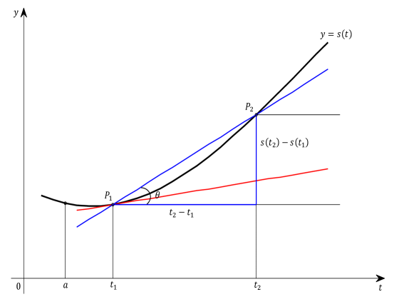
The instant speed at a time, say $t_{1}$ , is approximately the average speed in an ever smaller interval $[t_{1},t_{2}]$ , which means $t_{2}$ goes to $t_{1}$ . The limit expression is

\lim_{t_{2}\to t_{1}}\frac{s(t_{2})-s(t_{1})}{t_{2}-t_{1}}=v(t_{1}).

(10)

This is regarded as the slope of $y=s(t)$ at $t_{1}$ , i.e., the slope of the tangent line (i.e., the red line in Figure 5) of $y=s(t)$ at $t_{1}$ . We would like to show that $s(t)$ is an antiderivative of $v(t)$ , i.e., $s(x)=I[v(t),0,x]$ . We divide $[0,x]$ uniformly into $n$ sub-intervals of width $h=x/n$ . Within interval $[x_{i},x_{i+1})$ , the distance traveled is approximately $v(x_{i})h$ . The total distance traveled in $[0,x]$ is $\sum_{i=1}^{n}v(x_{i})h$ , which goes to $s(x)-s(0)=I[v,0,x]$ as $n\to\infty$ . Thus, $(v(t),s(t))$ is a DA pair, i.e., the derivative of distance with respect to time is speed, and the integral of speed is the total distance traveled. Equation (10) provides another way of defining derivative in addition to the derivative introduced via DA pair. This definition of derivative by limit in (10) is the most popular way of introducing derivatives in today’s classrooms. It is also the main idea of Isaac Newton (1642-1727)’s approach to fluxion (see [7] for his book of Method of Fluxion, 1736). Before Newton, Pierre de Fermat (1601-1665) developed a method of tangents in 1629 using a small increment (i.e., infinitesimal) which is finally set to be zero when the infinitesimal disappears from the denominator (see [2, 3] ). Newton’s method of fluxion or tangent is similar to Fermat’s but introduced the concept of limit, although he did not explicitly use a mathematical notation or formula to express the limit [See [8] for his book “The Mathematical Principles of Natural Philosophy” (1729, p45)].

In summary, a derivative of $F(x)$ is a limit of its graphic mean. One can use the formulas of DA pairs given in the last section to find the derivative of a given function. For example, to find the derivative of $x^{2}$ , we use the DA pair $(x^{n},x^{n+1}/{n+1})$ . With $n=1$ , the pair becomes $(x,x^{2}/2)$ . So $(x^{2}/2)^{\prime}=x$ , hence $(x^{2})^{\prime}=2x$ .

6 Conclusions and discussion

We have used arithmetic mean to define integral. This definition leads to the DA pair concept, integral’s area meaning, and FTC. We have used graphic mean to interpret the meanings of a derivative as the slope of a curve or speed of moving object. The graphic mean also provides another way of calculating derivative by limit, an application of Fermat’s method of tangents. Computer calculation for DA pairs is used here in place of traditional derivation of derivative formulas using limit and graphic mean. Before today’s popularity of computer and internet, the method of introducing derivative by limit was very useful in the calculation of calculus problems, since the method can easily be used to derive various kinds of derivative formulas for non-polynomial functions, compared to the DA pair approach $I[f,0,x]$ . However, with today’s easy access to notebook computers, smart phones, and publicly available software, finding derivatives and integrals for a given function can be readily done on the internet. Thus, today’s calculus teaching may shift its emphasis from the limit-based hand calculations to the web-based calculations, concepts, interpretations, and applications. Limit is a difficult, subtle, puzzling and intermediate procedure for calculus. Although in our statistics calculus here the limit notation is introduced to state the existence of the arithmetic mean following LLN, we hardly used the concept of limit in formulation derivations and actual calculations. Statistical calculus’ rigorous background needs LLN, which requires a rigorous proof but its conclusion has a certain degree of intuition and can be treated as an axiom like those in Euclidean geometry. Thus, the calculus based on LLN implies that, with today’s handy computer technology, the calculus basics can be axiomized and the calculus method can be developed directly with minimum and intuitive theory without the need of some unnecessary, intermediate and complex procedures. In this way, calculus can be properly taught in high schools or in a workshop of a few hours as proposed in Ref. [6].

Acknowledgments. This research was supported in part by the US National Science Foundation. The opinions expressed do not necessarily reflect the views of the funding agencies. Nancy Tafolla helped calculate the data in Table 2. Discussions with Qun Lin of Chinese Academy of Sciences were useful for the development of this paper.

References