Black hole thermodynamics as seen through a microscopic model of a relativistic Bose gas

Abstract

Equations of gravity when projected on spacetime horizons resemble Navier-Stokes equation of a fluid with a specific equation of state [1, 2, 3]. We show that this equation of state describes massless ideal relativistic gas. We use these results, and build an explicit and simple molecular model of the fluid living on the Schwarzschild and Reissner-Nordström black hole horizons. For the spin zero Bose gas, our model makes two predictions: (i) The horizon area/entropy is quantized as given by Bekenstein’s quantization rule, (ii) The model explains the correct type of proportionality between horizon area and entropy. However, for the physically relevant range of parameters, the proportionality constant is never equal to $1/4$.

1 Introduction

There exists a popular viewpoint that general relativity, like fluid mechanics, could be seen as a thermodynamical equilibrium, macroscopic description of a system with completely different microscopic degrees of freedom. The idea traces back to Sakharov [4], however, in the last two decades there has been a surge of activities in this direction, see, for instance, Refs. [5, 6, 7, 8]. Similar ideas also form the core of the analogue gravity program (see, for instance, the review [9]).

Three decades ago, Damour [1] showed that the equations of general relativity when projected onto a black-hole horizon give Navier-Stokes equation of a 2-dimensional fluid that lives on the black hole horizon. This allowed Damour to identify various black hole properties with the properties of a 2-dimensional fluid. (For details on how the various fluid characteristics arise from the spacetime metric see the above reference.) This approach has now been generalized to arbitrary space-time horizons in recent works of Padmanabhan [2, 3]. (For other results on fluid-gravity correspondence see Refs. [10, 11, 12].) In case the results of [1, 2, 3] are not only a curious analogy, one expects that also properties of semi-classical black holes could be holographically obtained from statistical mechanics of the (quantum) (2 + 1)-dimensional fluid living on the black hole horizon.

In this work, we use results of Refs. [2, 3] and build an explicit and simple molecular model of the (2+1)-dimensional fluid. We show that the microscopic fluid model indeed provides a holographic analogue for different phenomena in semi-classical quantum gravity, bringing very interesting insights into the nature of various aspects of black hole thermodynamics. For example, the microscopic model presented here sheds some light on the proportionality between horizon area and entropy, and provides very interesting alternative explanation for the Bekenstein quantization of horizon area (or entropy) [13]. For the sake of simplicity, we consider in this work Schwarzschild and Reissner-Nordström black holes.

There have been attempts to build microscopic models describing physics of black hole horizons. (Microscopic models outside models of quantum gravity, such as String Theory, or Loop Quantum Gravity.) Specifically, in Ref. [14], the authors have used Bose-Einstein condensate as a microscopic model to describe black hole horizon as a surface of quantum phase transition. In this work, we also use a model of Bose gas, however our approach and its origins are very different from the one in Ref. [14].

In the next section, we use a molecular model to build an analogue for the thermodynamics of 4-D Schwarzschild black-hole. In section 3, we use a similar model to build an analogue for the thermodynamics of 4-D Reissner-Nordström black-hole. Finally, we end with discussion and some suggestions for future work.

In this work we use the metric signature $(-,+,+,+)$ and set $G=c=\hbar=k_{B}=1$.

2 The molecular model for the thermodynamics of Schwarzschild black hole

2.1 Model set-up

Damour-Navier-Stokes equation is obtained by projecting Einstein’s equations on the horizon and it identifies the fluid’s pressure with the horizon parameters as [2]

$$p=\frac{\kappa}{8\pi}=\frac{T_{H}}{4}.$$ (1)

($\kappa$ is the horizon surface gravity, assumed here to be positive, and $T_{H}$ is the Hawking temperature of the horizon.) This result relating fluid’s pressure and horizon’s surface gravity holds true for a general null surface [2] and is also shown to hold from purely thermodynamic reasons by identifying the temporal rate of change of Einstein gravity action with the spacetime entropy production [3]. The equation of state of the fluid (1) will be the starting point of this work.

Let us note that for the Schwarzschild black hole the above expression can be somewhat naively derived from the definition of pressure using the black hole entropy,

$$p=\frac{\partial S_{H}}{\partial A_{H}}\cdot T_{H}=\frac{T_{H}}{4}.~{}~{}~{}$$ (2)

Eq. (2) boils down to the fact that for Schwarzschild black hole:

$$dM=p\cdot dA_{H}=p\cdot dV.$$ (3)

In order to find the link to underlying microscopic theory, it is natural that we are interested in stationary configurations of the fluid. Stationary fluid configurations then naturally link to horizons generated by null Killing field. However, there is one more essential reason why to focus on Killing horizons and this is the fact that in order to find some potentially interesting microscopic model, we need to understand what is fluid’s energy. The natural concept for the energy of the fluid is the concept of Komar energy, but Komar energy is defined only for stationary spacetimes. Therefore it is essential that we restrict ourselves to stationary configurations and Killing horizons. We will discuss this more in the Discussion section.

As a consequence of what was said we do the following general assumptions that link the microscopic theory of the fluid to black hole thermodynamics, (these assumptions are consistent with the original paper of Damour [1]):

• since the fluid is a (2+1)-dimensional fluid living on a horizon, the volume of the fluid is naturally the area of the horizon $A_{H}$,

• the temperature of the horizon $T_{H}$ (with the chosen normalization of the time-like Killing field) is the temperature of the fluid,

• for fluid living on a Killing horizon, the total energy of the fluid is the horizon Komar energy.

(Later, it will be required for the entropy of the fluid to be identified with the black hole entropy.)

Now let us demonstrate that for a generic Killing horizon the equation of state (1) translates into equation of state of an ideal relativistic fluid. The Komar energy of the Killing horizon is computed from

$$E=-\frac{1}{8\pi}\int_{\mathcal{H}}\xi_{a;b}d\Sigma^{ab},$$ (4)

where $\xi$ is the suitably normalized Killing field generating the horizon. If the surface gravity of the horizon is positive, after short calculation one obtains

$$E=\frac{T_{H}V}{2}.$$ (5)

Combining Eq.(1) and Eq.(5) one gets

$$p=\frac{T_{H}}{4}=\frac{E}{2V}.$$

This is an equation of state of an 2D ideal massless relativistic gas [15].

Our aim is to identify a microscopic model for the Schwarzschild black hole using the fluid-gravity correspondence. For a microscopic theory defined by a Hamiltonian, the entropy is typically a function of three independent parameters $S(E,N,V)$, where $E$ is system’s energy, $N$ is the number of particles and $V$ is the volume. In what will follow we utilize some aspects of the microcanonical ensemble approach. For example the concept of temperature used in the following section will be defined as in the microcanonical ensemble, that is, knowing $S(E,N,V)$ we will fix $N,V$ and define $T=dE/dS$. However, the parameter space of Schwarzschild black hole is one-dimensional and can be expressed by a single parameter $V=A_{H}$ (or $E$.) Therefore, if a microscopic model is supposed to reproduce Schwarzschild black hole, one needs to constrain the space of states of the fluid to only one dimension. This means from the point of view of the relevant states of the system we will not treat the variables $E,N,V$ as independent, but they must fulfil two constrains: $E=E(V)$ and $N=N(V)$.

We can obtain the constrains as follows: If we interpret the fluid energy as the Komar energy and the volume as the horizon area, they must fulfil the relation imposed by the Schwarzschild solution:

$$V=16\pi E^{2}.$$ (6)

This means Eq.(6) provides the constrain $E=E(V)$. The second constraint $N=N(V)$ can be derived from the other well known equation, relating the mass of the black-hole and Hawking temperature:

$$E=\frac{1}{8\pi T_{H}}.$$ (7)

However, to derive $N(V)$ from Eq. (7), requires information about the microscopic model, and therefore it will be done later. At this stage all one needs to keep in mind is that the fluid’s parameter space is fully constrained to one dimension by Eq.(6) and Eq.(7). Furthermore, the constraints mean that for a specific value of $V$ only a specific combination of thermodynamical potentials $p,\mu,T$ is allowed.

In the first half of this section we have shown that the fluid is an ideal massless relativistic gas. The relativistic gas can be either Bose or Fermi. In the rest of this section, we show that the microscopic model of a massless Bose gas living on a sphere predicts the form of $N(V)$ that leads to the Bekenstein’s black-hole area quantization [13].

2.2 The microscopic description (from the microcanonical point of view)

Now let us have a better look at the consequences of the ideal gas model. The energy levels of a free non-relativistic particles living on a sphere were calculated in [17, 18] as:

$$\epsilon^{nr}_{\ell}=\frac{\ell(\ell+1)+\alpha^{2}}{2R^{2}}$$ (8)

where $R$ is a radius of the sphere and $\alpha^{2}$ is some constant. (In a strict sense there are differences between [17] and [18] on whether the constant is allowed to be non-zero. However any energy quantum spectrum can be always shifted by a constant, which in best case is fixed by gravity considerations, such as these, so physically we stick to the spectrum given by Eq.(8) with arbitrary $\alpha$.) The energy levels correspond to the Laplacian on the sphere and therefore have the degeneracy of the spherical harmonics, given as $g_{\ell}=2\ell+1$.

As one can see from the Hamiltonian used in [17], we can obtain spectrum of a massless relativistic scalar particle by a simple transformation:

$$\epsilon^{r}_{\ell}=\sqrt{2\epsilon^{nr}}=\frac{\sqrt{\ell(\ell+1)+\alpha^{2}}}{\sqrt{2}\cdot R}=\sqrt{\frac{4\pi\{\ell(\ell+1)+\alpha^{2}\}}{V}}.$$ (9)

This can be (through our constrains) expressed as a simple function of temperature

$$\epsilon^{r}_{\ell}=\sqrt{\{\ell(\ell+1)+\alpha^{2}\}}\cdot T=\tilde{\epsilon}_{\ell}\cdot T,$$ (10)

with

$$\tilde{\epsilon}_{\ell}=\sqrt{\ell(\ell+1)+\alpha^{2}}.$$

($\tilde{\epsilon}_{\ell}$ is independent on the black hole parameters.) For simplicity, in this work, we utilize the spectrum (10) and we model the ideal relativistic massless gas by particles with zero spin, which also means we work with Bose gas.

We have constrained our system by equations (6) and (7). One of those equations gives the constraint $E(V)$, the other equation then implies another constraint $N(V)$. Let us now obtain the constraint $N(V)$: Note that in a microcanonical ensemble when $T$ is much larger than spacing between the quantum energy levels, the mean particle’s energy linearly decreases with temperature, as prescribed by the equipartition law. It can be shown for a simple harmonic oscillator that the equipartition law ceases to hold for very low temperatures, when the temperature is of a comparable value to the discrete spacing between the energy levels. Furthermore, for temperatures of a value comparable to the spacing between the energy levels the average particle’s energy is very close to the ground state energy. From Eq.(10) one observes that, in our constrained system, the temperature always is of a comparable value to the spacing between the energy levels, which means the equipartition law is not applicable.

This in turn implies that our free gas is supposed to have mean particle’s energy very near the ground state. In such case we can use the spectrum (10) to see that the mean particle’s energy must be:

$$\bar{E}=\gamma\cdot T,$$

where $\gamma\geq|\alpha|$ and $\gamma$ being approximately of the same order as $|\alpha|$. Since

$$E=N\bar{E}=N\gamma\cdot T\equiv(8\pi T)^{-1},$$

this implies

$$N=\frac{1}{8\pi\gamma T^{2}}=\frac{A_{H}}{2\gamma}.$$

Therefore

$$A_{H}=2\gamma\cdot N.$$ (11)

Eq.(11) is the desired second constraint $N(V)$. This is one of the main results of this work, and we would like to stress the following points:

• The derivation of $N(V)$ is based on few insights and presuppositions in the microcanonical ensemble approach. In the following section, we derive the same result more rigorously. In particular, in the next section, we will use the result given by Eq.(11) as an Ansatz and it will be shown that the Ansatz is correct in the sense that it fulfils all the constrains of the model. This means the relation (11) is a direct consequence and prediction of our microscopic model.

• Eq.(11) is remarkable as it gives Bekenstein’s [13] quantization of the black hole horizon area (since $N$ is by definition a natural number). It gives a completely new and independent insight into Bekenstein’s result. Furthermore, the insight does not rely on the quantum theory, only on the fluid interpretation of gravity. (The constant $\gamma$ is here arbitrary, but can be fixed to obtain the most popular form of Bekenstein type of spectrum as $\gamma=4\pi$. Since it will be shown that $\gamma=|\alpha|$, it can be demonstrated that this fixing gives wave-length of the particle in the ground state equal to the circumference of the black hole horizon.) Note that the linear proportionality between the horizon area and the number of degrees of freedom is a starting assumption in the grand-canonical statistical analysis of Schwarzschild black hole in Ref. [19].

• The formula (11) has also a deeper meaning; it is problematic to speak about density of fluid’s degrees of freedom, as to speak about density one needs pre-defined geometry. However, geometry is in this view a macroscopic property constituted by the fluid. In some sense it is natural to fix the way how the geometry is constituted by the fluid by relating it to the density of the fluid’s degrees of freedom as:

  $$\frac{N}{A_{H}}=(2\gamma)^{-1}=const.~{}.$$

  This also explains why in the fluid-gravity approach one obtains analogue of Navier-Stokes equation [2] (and energy diffusion equation given by the Raychhadhuri equation), but not the (rest-)mass conservation equation. The fact that the particles are massless, and the density of particles is always the same constant, means that mass conservation equation is fulfilled by a simple identity (its information rests only in how geometry links to the fluid particles).

• One of the standard problems with black hole physics is the fact that black holes have usually negative heat capacity. This means for black holes one cannot define canonical partition function [20] and it seems black holes cannot be represented by well known microscopic models of a fluid. The key observation is that our model is very different: By fixing volume and the number of particles, and computing derivative of $E(T)$ one obtains positive heat capacity. However since our model is one-dimensional constrained model in which change in temperature leads simultaneously to change in all fluid parameters (energy, number of particles and volume), the derivative of $E(T)$ does not correspond to a standard notion of heat capacity and can be negative.

2.3 More rigorous statistical ensemble calculation

One can confirm the insights from the last section through a more rigorous statistical ensemble calculation of our constrained system. The calculation is a hybrid between canonical and grand-canonical ensemble, therefore we refer to it as statistical ensemble calculation. The number of particles is not kept fixed (which makes it look like grand-canonical ensemble), but the system is constrained to only one parameter (which we choose to be the energy), which makes it look as a canonical ensemble. We want to stress that our calculation is still semi-classical and therefore we assume our system to be in a sufficiently low temperature regime. (This is the regime of sufficiently large black holes where semi-classical description is reasonably close to the reality.) More precisely, the sufficiently low temperature regime means that $T/T_{p}<<1$, where $T_{p}$ is Planck temperature. Since we use Planck units, $T_{p}=1$, and therefore in Planck units the condition of semi-classicality translates to $T<<1$.

Let us start from the first principles and assume our system to be in a contact with a huge reservoir. Then the probability of a state with energy $E$ for a Bose system is given by:

$$p(E)\sim\Omega\{n_{\ell}\}\exp\left\{-\frac{dS(E,V(E),N(E))}{dE}\cdot E\right\}=~{}~{}~{}~{}~{}~{}~{}~{}~{}~{}~{}~{}~{}~{}~{}~{}~{}~{}~{}~{}~{}~{}~{}~{}~{}~{}~{}~{}~{}~{}~{}~{}~{}~{}~{}~{}~{}~{}~{}~{}~{}~{}~{}~{}~{}~{}~{}~{}~{}$$

$$\Omega\{n_{\ell}\}\exp\left\{-\frac{\partial S(E,V(E),N(E))}{\partial E}\cdot E-\frac{\partial S(E,V(E),N(E))}{\partial V}\frac{\partial V}{\partial E}\cdot E-\right.~{}~{}~{}~{}~{}$$ (12)

$$\left.\frac{\partial S(E,V(E),N(E))}{\partial N}\frac{\partial N}{\partial E}\cdot E\right\}=\Omega\{n_{\ell}\}\exp\left\{-\frac{E}{T}+f(T)\,\frac{\partial N}{\partial E}\cdot E\right\}=~{}~{}$$

$$\Omega\{n_{\ell}\}\exp\left\{-\frac{E}{T}+f(T)\,\frac{16\pi}{\gamma}\cdot E^{2}\right\}.~{}~{}~{}~{}~{}~{}~{}~{}~{}~{}~{}$$

Here

$$\Omega\{n_{\ell}\}=\prod_{\ell}\frac{(n_{\ell}+g_{\ell}-1)!}{n_{\ell}!(g_{\ell}-1)!}\quad~{}~{}\mbox{and}~{}~{}\quad f(T)=\frac{\mu-2\gamma p}{T},$$ (13)

with $g_{\ell}$ being the degeneracy of the energy level and $\mu$ chemical potential. The variables in Eq.(2.3) are subject to two constrains

$$\sum_{\ell}\epsilon_{\ell}n_{\ell}-E=0,$$ (14)

and

$$\sum_{\ell}n_{\ell}-N=\sum_{\ell}n_{\ell}-\frac{8\pi E^{2}}{\gamma}=0.$$ (15)

In constraint (15) we substituted for $N$ a function of $E$ using Eq.(11) and Eq.(6).

For $n_{\ell}>>1$ one can use Stirling’s formula and transform Eq.(2.3) to:

$$p(E)\sim\exp\left(-\frac{E}{T}+\frac{16\pi f(T)E^{2}}{\gamma}+\right.~{}~{}~{}~{}~{}~{}~{}~{}~{}~{}~{}~{}~{}~{}~{}~{}~{}~{}~{}~{}~{}~{}~{}~{}~{}~{}~{}~{}~{}~{}~{}~{}~{}~{}~{}~{}~{}~{}~{}~{}~{}~{}~{}~{}~{}~{}$$

$$+\left.\sum_{\ell}\left[(n_{\ell}+g_{\ell})\{\ln(n_{\ell}+g_{\ell})-1\}-n_{\ell}\{\ln(n_{\ell})-1\}-\ln([g_{\ell}-1]!)\right]\right).$$ (16)

If we assume that the value of $\bar{E}(T)$ is given by the extremum of $p(E)$, then we obtain using Lagrange multipliers the following equations

$$\frac{\partial}{\partial n_{\ell^{\prime}}}:~{}~{}~{}~{}\ln\left(\frac{n_{\ell^{\prime}}+g_{\ell^{\prime}}}{n_{\ell^{\prime}}}\right)+\tilde{\lambda}\cdot\epsilon_{\ell^{\prime}}+\lambda=0,$$

$$\frac{\partial}{\partial E}:~{}~{}~{}~{}-\frac{1}{T}+\frac{32\pi f(T)E}{\gamma}-\tilde{\lambda}-\frac{16\pi E\lambda}{\gamma}=0,$$

$$\frac{\partial}{\partial\tilde{\lambda}}:~{}~{}~{}~{}\sum_{\ell}\epsilon_{\ell}n_{\ell}-E=0,$$

$$\frac{\partial}{\partial\lambda}:~{}~{}~{}~{}\sum_{\ell}n_{\ell}-\frac{8\pi E^{2}}{\gamma}=0.$$

Here $\tilde{\lambda}$ and $\lambda$ are Lagrange multipliers corresponding to the two constraints (14) and (15). Take the first equation and substitute for $\tilde{\lambda}$ from the second equation to obtain:

$$\bar{n}_{\ell^{\prime}}=\frac{g_{\ell^{\prime}}}{\exp\left(\left[\frac{16\pi E\lambda}{\gamma}+\frac{1}{T}-\frac{32\pi f(T)E}{\gamma}\right]\epsilon_{\ell^{\prime}}-\lambda\right)-1}.$$ (17)

Let us further use the fact that $E$ must be a function of temperature given by Eq.(7). Then equation (17) can be rewritten as

$$\bar{n}_{\ell^{\prime}}=\frac{g_{\ell^{\prime}}}{\exp\left(\left[\frac{2\lambda}{\gamma}+1-\frac{4f(T)}{\gamma}\right]\tilde{\epsilon}_{\ell^{\prime}}-\lambda\right)-1}.$$ (18)

($\tilde{\epsilon}_{\ell^{\prime}}$ was defined before and is independent on external parameters.)

Before we proceed, it may be worth pointing out that the equation (18) has certain limitations. The limitations arise due to the use of Stirling’s approximation and the fact that in general for higher occupation numbers (where the numbers are small) the above formula could give inaccurate results. Despite some quantitative modifications (due to changes in the asymptotic behavior of $\bar{n}_{\ell}$), in most of the cases one can still expect that the exact results go qualitatively along similar lines as the ones derived via Eq.(18). For example constrains (14) and (15) could fix (slightly different) $\gamma(\alpha)$ and $f(T)$, however, the final conclusions can be expected to remain unchanged.

A necessary condition for every occupation number is that it is positive for each level. This leads to the condition

$$\frac{2\lambda}{\gamma}+1-\frac{4f(T)}{\gamma}\geq 0~{}~{}~{}~{}~{}~{}\forall\,\,T.$$ (19)

Now let us explore the possibilities of obtaining divergent number of particles for the asymptotic case $T=0$. (This is a necessary condition that our model must fulfil and means that in the limiting case of zero temperature it corresponds to a black hole with infinite horizon area and infinite mass.) One possibility would be that

$$\frac{2\lambda}{\gamma}+1-\frac{4f(0)}{\gamma}=0,$$

and $\lambda\leq 0$, which would lead to a constant finite non-zero distribution of particles over states. This, however, would contradict our assumption that the average particle’s energy is close to the ground state.

The only remaining possibility (how to obtain the infinite number of particles) is if the infinite number of particles are specifically in the ground state. This happens if:

$$\lambda=\frac{(4f(0)-\gamma)|\alpha|}{2|\alpha|-\gamma}.$$

One can then easily derive from Eq.(18) that:

$$0<\sum_{\ell=1}^{\infty}\bar{n}_{\ell}<\infty~{}~{}~{}\hbox{as}~{}~{}~{}T=0.$$ (20)

where $n_{0}$ would be the occupation number of the ground state $\ell=0$. Since also $\sum_{\ell=1}^{\infty}\tilde{\epsilon}_{\ell}\bar{n}_{\ell}$ (the sum of energies above the ground state energy) clearly converges, this means $\gamma=|\alpha|$ and

$$\lambda=4f(0)-|\alpha|.$$ (21)

It is important to realize that such a solution, represented by Eq.(21), can be always chosen for $\lambda$. This is because the only consistency conditions are the two constrains (14) and (15), in which constraint (14) only leads for $T<<1$ to our condition $\gamma=|\alpha|$ and the constraint (15) can always be fulfilled, since it just determines the correct choice of $f(T)$, which means the correct choice of the chemical potential.

Eq.(21) together with Eq.(19) gives the following condition on $f(0)$:

$$f(0)>\frac{\gamma}{4}=\frac{|\alpha|}{4}.$$ (22)

Eq.(18) can be further rewritten as

$$\bar{n}_{\ell^{\prime}}=\frac{g_{\ell^{\prime}}}{\exp\left(\left[\frac{8f(0)}{|\alpha|}-1-\frac{4f(T)}{|\alpha|}\right]\tilde{\epsilon}_{\ell^{\prime}}-4f(0)+|\alpha|\right)-1},$$ (23)

which gives in the $T=0$ asymptotic case

$$\bar{n}_{\ell^{\prime}}=\frac{g_{\ell^{\prime}}}{\exp\left(\left[-1+\frac{4f(0)}{|\alpha|}\right]\tilde{\epsilon}_{\ell^{\prime}}-4f(0)+|\alpha|\right)-1}.$$ (24)

Now with these observations one can fix the function $f(T)$ through Eq.(15). If $T<<1$ the following equation is satisfied:

$$N\approx\frac{1}{\exp\{-4\cdot(f(T)-f(0))\}-1},$$

(the ground state is non-degenerate). This fixes

$$f(T)=f(0)-\frac{1}{4}\ln\left(1+\frac{1}{N}\right)=f(0)-\frac{1}{4}\ln\left(1+\frac{|\alpha|\cdot T^{2}}{2\pi}\right).$$

Therefore $[f(T)-f(0)]\in O(T^{2}).$

2.4 Calculating the entropy

There is one significant consistency check and this is the fact that we require the fluid’s entropy to match the black hole’s entropy. As previously mentioned, in the low-temperature limit we need to match the fluid entropy with the semi-classical black-hole thermodynamics results.

Let us use the first law of thermodynamics:

$$TdS=dE+p\cdot dV-\mu\cdot dN,$$ (25)

which leads to ($T$ small again)

$$dS=\frac{dE}{T}-f(T)\cdot dN\approx\frac{dE}{T}-\frac{2f(0)\cdot dE}{|\alpha|T}.$$

This automatically gives entropy to be proportional to the horizon area $\sim A_{H}$. However, claiming that entropy must be a growing function of $A_{H}$ gives the following upper bound on $f(0)$:

$$f(0)<\frac{|\alpha|}{2}.$$

Since the positivity of occupation numbers implies $f(0)>|\alpha|/4$, it means that $f(0)\in(|\alpha|/4,|\alpha|/2)$. This means the right proportionality given by $\sim 1/4$ cannot be reached as it would require $f(0)=0$. Therefore, our microscopic fluid model predicts that only part of the black hole entropy can be explained by the fluid. All this means is that our model indeed leads to the correct linear proportionality between entropy and the horizon area, but with a lower factor than $1/4$. (The proportionality factor depends on the free parameter $f(0)$ and lies in the interval $(0,1/8)$.) In Appendix A we suggest that similar entropy calculation excludes fermionic model.

One would possibly like to derive the same result in a more “proper” manner, from the statistical ensemble calculation. However, it is non-trivial to determine from the partition function what is the entropy of our system for $T<<1$. It is true that the degeneracy of the ground state, in which dominant number of particles reside for $T=0$, is zero, however there are finite occupation numbers when $T=0$ for the higher energy levels. These occupation numbers contribute to non-zero entropy. To calculate the entropy (e.g if it is convergent, or divergent at $T=0$) from the statistical approach based on Eq.(2.3) seems to be impossible, as the approximations (e.g Stirling formula) used in this section fail for the higher level occupation numbers. Despite of this, let us make a qualitative observation that as $T$ approaches zero the higher level occupation numbers grow (and approximate a finite constant value) and therefore entropy grows as $T\to 0$. This is consistent with what one observes for Schwarzschild black hole.

In the next section, we repeat the above analysis for Reissner-Nordström black-hole and show that we get the correct proportionality constant for certain range of $|Q|/M$.

3 The molecular model for the thermodynamics of Reissner-Nordström black hole

3.1 Model set-up

Reissner-Nordström black hole is a well known spherically symmetric static solution of Einstein equations in electrovacuum. The spacetime is labelled by two diffeomorphism invariant parameters $M,Q$, where $Q$ is the electromagnetic charge. For $0<|Q|/M<1$ the idealized mathematical solution has two horizons, the outer black hole, and the inner, Cauchy horizon. Following the idea that thermodynamical properties of horizons are universal [21, 22] we will consider thermodynamics of both the horizons in question. (Since the interest of this work are principal questions on how idealized thermodynamical properties of horizons could be explained by thermodynamical properties of fluid, we will take the inner horizon for this purpose seriously and omit the discussion of its physical relevance and instability.)

Let us denote the two horizons with the $\pm$ notation, where the symbol “$+$” symbolizes the outer and the symbol “$-$” symbolizes the inner horizon. In this section, we will derive the fluid microscopic model for both of the horizons simultaneously, however one has to keep in mind that the model of the fluid living at the outer horizon and the model of the fluid living at the inner horizon are two separate models.

Let us repeat and slightly update the connections between fluid and black hole properties (suggested already by original Damour paper [1]) that were made in the previous section:

• The fluid’s energy is the Komar energy of the horizon.

• The fluid’s temperature is the temperature associated with the horizon.

• The fluid’s volume is the area of the horizon. Since the horizon area will represent the 2D volume of the fluid, we denote it by the letter(s) $V_{\pm}$, rather than using the usual notation.

• The black hole charge is the charge of the fluid.

Again, the equation of state for free relativistic gas, that was derived in previous section for horizons with positive surface gravity can be demonstrated to hold true for fluid living on each of the horizons. (In the Reissner-Nordström case the assumption that surface gravity is positive no longer holds true for the inner horizon, but as we will further demonstrate, negative surface gravity still gives the same fluid’s equation of state.) Taking the horizon temperatures to be

$$T_{\pm}=\frac{|\kappa_{\pm}|}{2\pi},$$

where $\kappa_{\pm}$ are the surface gravities, the equation of state for the fluid on the horizon turns to be

$$p_{\pm}=\pm\frac{T_{\pm}}{4}.$$ (26)

The Komar energies calculated from the usual formula (4) are given by Smarr-type of formula:

$$E_{\pm}=\pm\frac{T_{\pm}V_{\pm}}{2}.$$ (27)

Then the equation of state (26) together with (27) implies for both horizons the same result as in the previous section:

$$p_{\pm}=\frac{E_{\pm}V_{\pm}}{2}.$$ (28)

This means the equation of state (28) holds generally for Einstein gravity, irrespective of whether horizon’s surface gravity is positive, or negative.

Let us end this part by introducing few useful relations. The horizon areas can be expressed as

$$V_{\pm}=4\pi\cdot(M\pm\sqrt{M^{2}-Q^{2}})^{2},$$ (29)

from which one can derive the following:

$$M=\sqrt{\frac{\pi}{V_{\pm}}}\cdot\left(\frac{V_{\pm}}{4\pi}+Q^{2}\right).$$ (30)

Further one can calculate

$$\sqrt{M^{2}-Q^{2}}=\pm\frac{1}{4\pi}\sqrt{\frac{\pi}{V_{\pm}}}\cdot(V_{\pm}-V_{ext}),$$ (31)

with $V_{ext}$ being horizon area in the extremal case ($|Q|=M$), therefore $V_{ext}=4\pi Q^{2}$. The horizon temperatures are given by:

$$T_{\pm}=\frac{2\sqrt{M^{2}-Q^{2}}}{V_{\pm}}=\pm\frac{1}{2\pi}\sqrt{\frac{\pi}{V_{\pm}}}\left(1-\frac{V_{ext}}{V_{\pm}}\right),~{}~{}~{}$$ (32)

and Komar energies $E_{\pm}$ are given by:

$$E_{\pm}=\pm\frac{V_{\pm}T_{\pm}}{2}=\pm\sqrt{M^{2}-Q^{2}}=\frac{1}{4\pi}\sqrt{\frac{\pi}{V_{\pm}}}\cdot(V_{\pm}-V_{ext}).$$ (33)

3.2 Microscopic description (from the microcanonical point of view)

Let us again consider that the energy spectrum of relativistic ideal gas living on a sphere is given by Eq.(9), with some ground state energies $\alpha_{\pm}$. Now repeat the arguments from the Schwarzschild case: The energy spectrum spacing behaves for fixed EM charge as $\sim V^{-1/2}$ and from (32) we can again observe that the temperature is always comparable to the energy level spacing. This means that equipartition theorem does not apply. This is in fact good news, as the Komar energy of the inner horizon is always negative, which cannot be explained by equipartition theorem, but can be explained if the ground state energy of the gas on the inner horizon has a negative value. (This means $\alpha_{-}<0$.)

Analogous to the Schwarzschild case, let us consider that the state of microcanonical ensemble for each horizon is described by four parameters $E_{\pm}$, $Q$, $N_{\pm}$, $V_{\pm}$. However, since we know that Reissner-Nordström black hole is only a two parametric model, we will need two constraints that reduce the dimension of the space of fluid states to two dimensions. Both of these constraints will be obtained in a complete analogy to the Schwarzschild case from the previous section. The first constraint is in fact the equation (33). For the second constraint one can use the equation (32). However, as in the previous Schwarzschild case, we would like to obtain constraints as translated to the language of $E_{\pm}$, $Q$, $N_{\pm}$, $V_{\pm}$. We use again insight telling us that for the relevant values of temperatures $T_{\pm}$:

$$E_{\pm}=\pm\frac{\tilde{\gamma}_{\pm}(Q)\cdot N_{\pm}}{\sqrt{V_{\pm}}},~{}~{}~{}~{}N_{\pm}\in\mathbb{N}$$ (34)

where $\tilde{\gamma}_{\pm}(Q)>0$. Eq. (33) implies:

$$2\gamma_{\pm}(Q)N_{\pm}=\pm(V_{\pm}-V_{ext})=|V_{\pm}-V_{ext}|,$$ (35)

with $\gamma_{\pm}(Q)=2\sqrt{\pi}\cdot\tilde{\gamma}_{\pm}(Q)$. One can also express $N_{\pm}$ more conveniently through $E_{\pm}$ as:

$$N_{\pm}=\pm\frac{4\pi}{\gamma_{\pm}}\left(E_{\pm}^{2}+E_{\pm}\sqrt{E_{\pm}^{2}+Q^{2}}\right).$$ (36)

Eq.(35) is an interesting generalization of Schwarzschild result showing that for a fixed charge ($Q$), the spectrum distancing the outer/inner horizon area from the extremality is equispaced. (Similar results were obtained via very different methods also in [23, 24].) Also, as intuitively expected, the non-statistical limit $N_{\pm}\to 0$ corresponds to extremality.

Let us briefly discuss $\gamma_{\pm}(Q)$ function and argue that it is in fact constant (independent on $Q$). The horizon is an equipotential surface and the charged two dimensional gas in an equilibrium state has on average zero potential energy. (This allows to model the equilibrium state as a free gas.) As a consequence, further in the calculations we assume that $\gamma_{\pm}$ is a constant and this leads to a natural Bekenstein-type generalization of the horizon area spectrum from the Schwarzschild case. (This is because the spacing in the area spectrum can be in such case, for $\gamma_{+}=\gamma_{-}$, a “universal” quantity.) The spectrum (35) is to some extend an Ansatz, but again, in analogy to Schwarzschild case it will be shown later in the section that it satisfies our microscopic model. Therefore it is indicated by this paper that, as shown more times before (see for example [22]), Bekenstein spectra for horizon area/entropy are a robust result. (In this case they also hold true for the inner Reissner-Nordström black hole horizon.)

3.3 More rigorous statistical calculation

We continue with generalization of the calculations from the previous section. We keep here the number of particles non-fixed, however the system is still subject to two constraints (33) and (35). As before, the probability distribution over states with energies $E_{\pm}$ is:

$$p(E_{\pm})\sim\Omega\{n_{\ell}\}\exp\left\{-\left(\frac{\partial S_{\pm}(E_{\pm},Q,V_{\pm}(E_{\pm},Q),N_{\pm}(E_{\pm},Q))}{\partial E_{\pm}}\cdot E_{\pm}+\right.\right.~{}~{}$$

$$\left.\left.+\frac{\partial S_{\pm}(E_{\pm},Q,V_{\pm}(E_{\pm},Q),N_{\pm}(E_{\pm},Q))}{\partial Q}\cdot Q\right)\right\}=~{}~{}~{}~{}~{}~{}~{}$$ (37)

$$=\Omega\{n_{\ell}\}\exp\left\{-\frac{E_{\pm}}{T_{\pm}}+f_{\pm}(T_{\pm},\phi_{\pm})\,\left(\frac{\partial N_{\pm}}{\partial E_{\pm}}\cdot E_{\pm}+\frac{\partial N_{\pm}}{\partial Q}\cdot Q\right)+\frac{\phi_{\pm}}{T_{\pm}}\cdot Q\right\}.~{}$$

Here, again,

$$\Omega\{n_{\ell}\}=\prod_{\ell}\frac{(n_{\ell}+g_{\ell}-1)!}{n_{\ell}!(g_{\ell}-1)!}$$ (38)

and

$$f_{\pm}(T_{\pm},\phi_{\pm})=\frac{\mu_{\pm}-2\gamma_{\pm}p_{\pm}}{T_{\pm}},$$ (39)

with $g_{\ell}$ being the degeneracy of the energy level and $\mu$ chemical potential. The thermodynamical potential related to $Q$ is

$$\phi_{\pm}=-T_{\pm}\frac{\partial S_{\pm}}{\partial Q},$$

which for the Reissner-Nordström solution and the outer horizon gives the electrostatic potential value at the outer horizon (at the inner horizon it gives the potential with the opposite sign). We also omitted the $\pm$ subscripts in case of $n_{\ell}$, (for keeping the notation less complicated), but they are implicitly assumed. The variables in Eq.(3.3) are subject to two constrains

$$\sum_{\ell}\epsilon_{\ell}n_{\ell}-E_{\pm}=0,$$ (40)

and

$$\sum_{\ell}n_{\ell}-N_{\pm}=\sum_{\ell}n_{\ell}\mp\frac{4\pi}{\gamma_{\pm}}\left(E_{\pm}^{2}+E_{\pm}\sqrt{E_{\pm}^{2}+Q^{2}}\right)=0.$$ (41)

For $n_{\ell}>>1$ one can use Stirling’s formula and transform Eq.(2.3) to:

$$p(E_{\pm})\sim\exp\left(-\frac{E_{\pm}-\phi_{\pm}Q}{T_{\pm}}+f_{\pm}(T_{\pm},\phi_{\pm})\left(E_{\pm}\frac{\partial N_{\pm}}{\partial E_{\pm}}+Q\frac{\partial N_{\pm}}{\partial Q}\right)+\right.~{}~{}~{}~{}~{}~{}~{}~{}~{}~{}~{}~{}~{}~{}$$

$$\left.\sum_{\ell}\left[(n_{\ell}+g_{\ell})\{\ln(n_{\ell}+g_{\ell})-1\}-n_{\ell}\{\ln(n_{\ell})-1\}-\ln([g_{\ell}-1]!)\right]\right).~{}~{}$$ (42)

If we assume that the value of $\bar{E_{\pm}}(T_{\pm})$ is given by the extremum of $p(E_{\pm})$, then we obtain using Lagrange multipliers the following equations

$$\frac{\partial}{\partial n_{\ell^{\prime}}}:~{}~{}~{}~{}\ln\left(\frac{n_{\ell^{\prime}}+g_{\ell^{\prime}}}{n_{\ell^{\prime}}}\right)+\tilde{\lambda}\cdot\epsilon_{\ell^{\prime}}+\lambda=0,$$

$$\frac{\partial}{\partial E_{\pm}}:~{}~{}~{}~{}-\frac{1}{T_{\pm}}+f_{\pm}(T_{\pm},\phi_{\pm})\frac{\partial}{\partial E_{\pm}}\left(\frac{\partial N_{\pm}}{\partial E_{\pm}}E_{\pm}+\frac{\partial N_{\pm}}{\partial Q}Q\right)-\tilde{\lambda}_{\pm}-\frac{\partial N_{\pm}}{\partial E_{\pm}}\lambda_{\pm}=0,$$

$$\frac{\partial}{\partial\tilde{\lambda}_{\pm}}:~{}~{}~{}~{}\sum_{\ell}\epsilon_{\ell}n_{\ell}-E=0,$$

$$\frac{\partial}{\partial\lambda_{\pm}}:~{}~{}~{}~{}\sum_{\ell}n_{\ell}\mp\frac{4\pi}{\gamma_{\pm}}\left(E_{\pm}^{2}+E_{\pm}\sqrt{E_{\pm}^{2}+Q^{2}}\right)=0,$$

$$\frac{\partial}{\partial Q}:~{}~{}~{}\frac{\phi_{\pm}}{T_{\pm}}+f_{\pm}(T_{\pm},\phi_{\pm})\frac{\partial}{\partial Q}\left(\frac{\partial N_{\pm}}{\partial E_{\pm}}E_{\pm}+\frac{\partial N_{\pm}}{\partial Q}Q\right)-\lambda_{\pm}\cdot\frac{\partial N_{\pm}}{\partial Q}=0.$$

Here $\tilde{\lambda}_{\pm}$ and $\lambda_{\pm}$ are Lagrange multipliers corresponding to the two constraints (40) and (41).

From the last equation one obtains

$$\lambda_{\pm}=\pm\frac{\gamma}{4\pi}\frac{\phi_{\pm}}{T_{\pm}}\frac{\sqrt{E_{\pm}^{2}+Q^{2}}}{E_{\pm}Q}+2f_{\pm}(T_{\pm},\phi_{\pm}),~{}~{}~{}~{}~{}Q\neq 0.$$ (43)

Similar to the Schwarzschild case, we get,

$$\bar{n}_{\ell^{\prime}}=\frac{g_{\ell^{\prime}}}{\exp\left(\left[\frac{[\lambda_{\pm}-f_{\pm}(T_{\pm}\phi_{\pm})]}{\sqrt{V_{\pm}}}\cdot\frac{\partial N_{\pm}}{\partial E_{\pm}}+\frac{1}{T_{\pm}\sqrt{V_{\pm}}}-\frac{f_{\pm}(T_{\pm},\phi_{\pm})}{\sqrt{V_{\pm}}}\left(\frac{\partial^{2}N_{\pm}}{\partial E_{\pm}^{2}}E_{\pm}+\frac{\partial^{2}N_{\pm}}{\partial E_{\pm}\partial Q}Q\right)\right]\tilde{\epsilon}_{\ell^{\prime}}-\lambda_{\pm}\right)-1}.$$

($\tilde{\epsilon}_{\ell^{\prime}}$ is defined as in previous section: $\tilde{\epsilon}_{\ell^{\prime}}=\sqrt{\ell^{\prime}(\ell^{\prime}+1)}\pm\alpha_{\pm}$.) Note that $\lambda_{\pm}$ can be rewritten through another free parameter $\phi$ via Eq.(43).

Let us now explore the general limit $Q^{2}/M^{2}\to K$ (where $0\leq K\leq 1$) and $T_{+}<<1$. Then within this limit, the following approximation is valid:

$$E_{\pm}\approx\pm M\sqrt{1-K}.$$

It can be further shown that in this limit ($T_{+}<<1$)

• $\frac{1}{T_{\pm}\sqrt{V_{\pm}}}\to C_{1\pm}\neq 0$,

• $\frac{\partial N_{\pm}}{\partial E_{\pm}}\frac{1}{\sqrt{V_{\pm}}}\to C_{2\pm}\neq 0,$

• $\left(E_{\pm}\frac{\partial^{2}N_{\pm}}{\partial E_{\pm}^{2}}+Q\frac{\partial^{2}N_{\pm}}{\partial E_{\pm}\partial Q}\right)\frac{1}{\sqrt{V_{\pm}}}\to C_{3\pm}\neq 0.$

($C_{1\pm}$, $C_{2\pm}$ and $C_{3\pm}$ are some constants defined by the limit and they will be later explicitly calculated.) If one again imposes that in the limiting case $T_{+}=0$, and $\phi_{\pm}=\phi_{0\pm}$ one will end up with infinite number of particles in the ground state, one obtains:

$$\lambda_{\pm}=\frac{(f_{\pm}(0,\phi_{0\pm})\{C_{2\pm}+C_{3\pm}\}-C_{1\pm})\alpha_{\pm}}{C_{2\pm}\alpha_{\pm}\mp 1}.$$

Parameter $\alpha_{\pm}$ comes from Eq.(9) and can be trivially shown in exact analogy to the Schwarzschild case to fulfil:

$$\alpha_{\pm}=\gamma_{\pm}.$$ (44)

This implies together with Eq.(35) the following inequality: $\alpha_{+}>0>\alpha_{-}$. (We will still use the $\alpha_{\pm}$ notation to distinguish it from $\gamma_{\pm}$, but we will use the Eq.(44) in the following calculations.)

The coefficients $C_{1\pm},C_{2\pm},C_{3\pm}$ can be calculated as:

$$C_{1\pm}=\frac{\sqrt{\pi}(1\pm\sqrt{1-K})}{\sqrt{1-K}},$$

$$C_{2\pm}=\pm\frac{2\sqrt{\pi}}{\gamma_{\pm}}\left(2-\frac{K(1+K)}{1\pm\sqrt{1-K}}\right),$$

$$C_{3\pm}=\pm\frac{2\sqrt{\pi}}{\gamma_{\pm}}\left(2-\frac{K}{1\pm\sqrt{1-K}}\right).$$

Assuming that $C_{2\pm}\alpha_{\pm}\mp 1>0$ and $C_{2+}+C_{3+}>0$ the positivity of the occupation number condition leads to:

$$f_{+}(0,\phi_{0\pm})>\frac{C_{1+}}{C_{2+}+C_{3+}}=\frac{\gamma_{+}(1+\sqrt{1-K})}{2\sqrt{1-K}\left(4-\frac{K(2+K)}{1+\sqrt{1-K}}\right)}>0,$$ (45)

and

$$f_{-}(0,\phi_{0\pm})<\frac{C_{1-}}{C_{2-}+C_{3-}}=-\frac{\gamma_{-}(1-\sqrt{1-K})}{2\sqrt{1-K}\left(4-\frac{K(2+K)}{1-\sqrt{1-K}}\right)}.$$ (46)

To determine the range of validity of the conditions $C_{2\pm}\mp 1>0$ and $C_{2\pm}+C_{3\pm}>0$ we needed to do some numerical calculations, as the expressions contain polynomials of higher than second order. Although these are in general analytically tractable, it is easier to calculate and plot the functions numerically. Our numerical calculations show the conditions $C_{2\pm}\alpha_{\pm}\mp 1>0$ and $C_{2+}+C_{3+}>0$ are always true for the relevant $K$. However the condition $C_{2-}+C_{3-}>0$ is violated for for $K\gtrapprox 0.85$. For this case the inequality given by Eq.(46) turns to be the opposite and gives a lower bound. For $K=0$, which is the most relevant case:

$$C_{1+}=2\sqrt{\pi},~{}~{}~{}~{}C_{2+}=C_{3+}=\frac{4\sqrt{\pi}}{\gamma_{+}},$$

and therefore

$$f_{+}(0,\phi_{0})>\frac{\gamma_{+}}{4}.$$

This is the Schwarzschild result from the previous section. We also see that the bounds on $f_{\pm}$ go to $\infty$ as we approximate the extremal case (which is however outside the scope of our approach).

Now consider the first law of thermodynamics and calculate the entropy:

$$dS_{\pm}=\frac{dE_{\pm}}{T_{\pm}}-f_{\pm}(T_{\pm},\phi_{\pm})dN_{\pm}-\frac{\phi_{\pm}}{T_{\pm}}dQ.$$ (47)

The first law of R-N black hole thermodynamics that comes from the “correct” entropy is:

$$dS_{\pm}=\pm\left(\frac{dM}{T_{\pm}}-\frac{\phi_{\pm}\cdot dQ}{T_{\pm}}\right)=2\pi M(1\pm\sqrt{1-K})^{2}dM.$$ (48)

The terms in Eq.(47) read as:

$$\frac{dE_{\pm}}{T_{\pm}}=\pm\frac{2\pi(1+K)(1\pm\sqrt{1-K})^{2}M}{\sqrt{1-K}}dM,$$

$$dN_{\pm}=\frac{8\pi}{\gamma_{\pm}}\sqrt{1-K}(1\pm\sqrt{1-K})MdM,$$

furthermore

$$\frac{\phi_{\pm}}{T_{\pm}}=\pm\frac{4\pi}{\gamma_{\pm}}\frac{M\sqrt{1-K}\sqrt{K}}{(C_{2\pm}\alpha_{\pm}\mp 1)}\left\{f_{\pm}(\Delta_{\pm}\alpha_{\pm}+2)-C_{1\pm}\alpha_{\pm}\right\},$$

with

$$\Delta_{\pm}=C_{3\pm}-C_{2\pm}=\pm\frac{2\sqrt{\pi}}{\gamma_{\pm}}\frac{K^{2}}{(1\pm\sqrt{1-K})}.$$

Then the first law of thermodynamics turns into:

$$dS_{\pm}=\left\{\pm\frac{(1\pm\sqrt{1-K})}{\sqrt{1-K}}\left((1+K)(1\pm\sqrt{1-K})+\frac{2\sqrt{\pi}\sqrt{1-K}\cdot K}{C_{2\pm}\alpha_{\pm}\mp 1}\right)-\right.~{}~{}~{}~{}~{}$$

$$\left.f_{\pm}(0,\phi_{0\pm})\cdot\frac{2\sqrt{1-K}}{\gamma_{\pm}}\left(2(1\pm\sqrt{1-K})\pm\frac{K(\Delta_{\pm}\alpha_{\pm}+2)}{C_{2\pm}\alpha_{\pm}\mp 1}\right)\right\}\cdot 2\pi M\cdot dM.~{}~{}$$ (49)

Now $f_{\pm}(0,\phi_{0\pm})$ is determined from equating the expressions on the right side of Eq.(48) and Eq.(3.3). One immediate minimal condition is that the entropy of the outer horizon grows with its area (the proportionality is a positive number):

$$\frac{(1+\sqrt{1-K})}{\sqrt{1-K}}\left((1+K)(1+\sqrt{1-K})+\frac{2\sqrt{\pi}\sqrt{1-K}\cdot K}{C_{2+}\alpha_{+}-1}\right)-~{}~{}~{}~{}~{}$$

$$f_{+}(0,\phi_{0+})\cdot\frac{2\sqrt{1-K}}{\gamma_{+}}\left(2(1+\sqrt{1-K})+\frac{K(\Delta_{+}\alpha_{+}+2)}{C_{2+}\alpha_{+}-1}\right)>0.$$ (50)

The same condition gives for the inner horizon:

$$-\frac{(1-\sqrt{1-K})}{\sqrt{1-K}}\left((1+K)(1-\sqrt{1-K})+\frac{2\sqrt{\pi}\sqrt{1-K}\cdot K}{C_{2-}\alpha_{-}+1}\right)-~{}~{}~{}~{}~{}$$

$$f_{-}(0,\phi_{0-})\cdot\frac{2\sqrt{1-K}}{\gamma_{-}}\left(2(1-\sqrt{1-K})-\frac{K(\Delta_{-}\alpha_{-}+2)}{C_{2-}\alpha_{-}+1}\right)<0.$$ (51)

For $K=0$ the condition (3.3) leads, as expected, to the Schwarzschild result:

$$f_{+}(0,\phi_{0+})<\frac{\gamma_{+}}{2}.$$

Also we can easily observe that the upper bound from Eq.(3.3) for $f_{+}(0,\phi_{0+})$ goes to $\infty$ as $K\to 1$ and the lower bound for $f_{-}(0,\phi_{0-})$ from Eq.(3.3) goes to $-\infty$. This is expected and consistent with the condition for positivity of occupation numbers for low $T_{+}$.

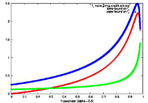
Figure 1: Plot showing the value of $f_{+}(0,\phi_{0+})$ for the correct proportionality of entropy and horizon area (red line), the lower bound on $f_{+}(0,\phi_{0+})$ (green line), and the upper bound on $f_{+}(0,\phi_{0+})$ (blue line). We see that the model is consistent (upper bound we get higher than lower bound).

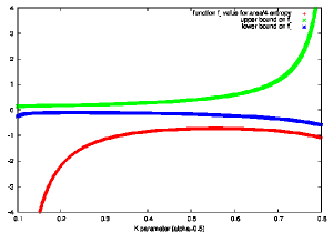
Figure 2: Plot showing the value of $f_{-}(0,\phi_{0-})$ for the correct proportionality of entropy and horizon area (red line), the lower bound on $f_{-}(0,\phi_{0-})$ (blue line), and the upper bound on $f_{-}(0,\phi_{0-})$ (green line). We see that the model is consistent (upper bound we get higher than lower bound).

Numerical analysis of conditions (45) and (3.3) for $f_{+}(0,\phi_{0+})$ is presented in Fig.(1). (We used $\alpha_{+}=0.5$, but since all the results depend linearly on $\alpha_{\pm}$, a concrete choice of $\alpha_{\pm}>0$ is irrelevant for the analysis.) We see that the theory is consistent in the sense that lower bound is always smaller than the upper bound, therefore there always exist a range of choices of $f_{+}(0,\phi_{0+})$ for which the theory is sensible. (These choices guarantee no negative occupation numbers and also the increase of entropy as proportional to the area of the horizon.) This is very important to know. The red line in Fig.(1) represents $f_{+}(0,\phi_{0+})$, such that leads to the correct proportionality between horizon area and entropy given by the factor $1/4$. As we see from Fig.(1), the choice leading to $1/4$ is possible only for $K\gtrapprox 2.7$ and for low charges $K\lessapprox 2.7$ one cannot obtain the correct proportionality $S=A/4$. This is consistent with what we observed for the Schwarzschild case ($K=0$).

The same investigation was done for the $f_{-}(0,\phi_{0-})$ function and is presented in Fig.(2). The numerical results show that for $K\lessapprox 0.1$ we obtain from both conditions (46) and (3.3) upper bounds on $f_{-}(0,\phi_{0-})$, therefore one can always fulfil these conditions. The same happens with lower bounds and $K\gtrapprox 0.85$ (both of the conditions lead for such $K$ to lower bounds). The relevant regime where we needed to explore the consistency of the theory is $0.1\lessapprox K\lessapprox 0.85$. In this regime the Fig.(2) indeed shows that the theory is consistent, since the upper bound is always larger than the lower bound. The red line represents again the value of $f_{-}(0,\phi_{0-})$ for the correct proportionality between area and entropy ($1/4$ factor) and in this case one sees from Fig.(2) that the correct proportionality cannot be reached for any value of $K$.

4 Discussion

We have shown that equation of state for the holographic fluid living on a spacetime horizon derived by [2] is for stationary configurations equal to an equation of state of an relativistic ideal gas. This provides better physical understanding of the nature of the fluid. Also the result is valid for generic spacetime horizon and depends only on General Relativity theory.

Many consequences of our microscopic holographic model for the black hole thermodynamics were discussed in the appropriate places in the text. The first main feature of our model is that it predicts for the black hole horizon an equispaced area / entropy spectrum. (There are many different arguments that lead to this type of spectrum that was originally suggested by Bekenstein [13]. For overview of these arguments see for example [22].) The spacing in the area spectrum is undetermined by our model, but it is equal to two times ground state energy of a single particle state. One can then proceed further and use either reduced quantization methods [23, 24], or quasinormal modes [25, 26] to fix the spacing between the area/entropy levels. The most widely agreed outcome will give in Planck units the area spacing as $8\pi$ and will lead to the one-particle’s ground state energy equal to $4\pi T$.

The second prediction is that we recovered with our model the correct type of proportionality between horizon area and entropy. However the proportionality factor is for Schwarzschild black hole less than one half of what is the result for black holes in Einstein gravity. (We have also shown that the correct proportionality can be reached in case of Reissner-Nordström black hole for sufficiently large $|Q|/M$ ratio.) One can try to “resolve” this problem by suggesting more species of particles whose entropy adds up to the correct proportionality, but this might sound slightly artificial without support of some additional arguments. Anyway, let us keep such a suggestion open for future investigations.

It is very important to realize some limitations of our approach: Standardly one can fully derive macroscopic fluid dynamics from a Hamiltonian of a microscopic theory. However despite of instructiveness of our model, this is not going to be possible with our microscopic model, at least not in the usual sense. One does not posses a local concept of energy in General Relativity in dynamical situations and this could pose a fundamental problem in deriving some local fluid dynamics from our (and any other similar) model. It is also clear that the model of free fluid would be unable to explain the dissipative terms that appear in the equations derived by Damour [1] and contribute significantly to the dynamics. So even if the energy problem was overcome one would expect that the “full” microscopic model will have some more complicated features and only in the limit of stationarity the EQS reduces to a free relativistic gas. To get an improved microscopic model from which full dynamics could be derived is an open problem.

There are many more open questions and problems, for example:

• We considered only the simplest, scalar (spin 0) Bose particle model. One does not assume any significant changes for bosons if higher spins $s=1,2$ were employed, but one needs to calculate the one-particle energy spectra for such cases. Suggesting that the spectra should be similar to the spectrum (9), one can also exclude half spin particles (fermions). This calculation is done in Appendix A. However all this needs to be further explored.

• Only the simplest models of Schwarzschild and Reissner-Nordström black holes were explored, it would be nice to see to what extent we can generalize the model to the stationary rotating (Kerr) black hole.

• Many results [3, 16, 22] suggest that distinguishing between black hole horizon and more general spacetime horizons is somewhat artificial. To what extent can our results be generalized beyond black holes? Also, since our results are for fundamental reasons non-local (energy spectra are a non-local quantity), is there still a chance to somehow reformulate the theory for a local Rindler horizon?

• Another question are generalized theories of gravity. Is a similar microscopic model applicable to black holes / horizons in generalized theories of gravity? The fact that in many generalized theories entropy follows Bekenstein quantization rules, but the horizon area does not [27], suggests that generalization within gravity theories might correspond to a generalization within fluid’s equation of state. Is this indeed true? Can one classify gravity theories by the equations of states of the fluid? The most straightforward generalization of Einstein equations, by introducing cosmological constant $\Lambda$, suggests that the answer is positive. It can be easily shown that the fluid’s equation of state acquires for the theory with $\Lambda$ an additional term proportional to $\sqrt{V}$:

  $$p=\frac{E}{2V}-\frac{\Lambda\sqrt{V}}{6(4\pi)^{3/2}}.$$

  Also some additional questions relating to what was previously said can be raised: For example, can one interpret the non-equilibrium thermodynamical effects that occur in higher curvature gravity [28, 29] through such a microscopic model of a suitable fluid?

• One can also stick to the model we have and further explore, and discuss, possible consequences of the model, such that could lead to potentially observable predictions.

Appendix A Fermionic model with energy spectrum (10)

Let us consider Schwarzschild black hole and fermions assuming that the one-particle energy spectrum will be the same as in case of zero spin particles, hence the spectrum is given by Eq.(10). [There will be small corrections due to the spin 1/2 nature, but in the present calculation they are not supposed to contribute.]

Let us first estimate the function $N(E)$ for temperatures so close to zero, that all the energy states up to Fermi level will be occupied by one particle, and the levels above will have zero occupation number. The energy can be calculated as:

$$E=\sum_{\ell=0}^{L}g_{\ell}\cdot\epsilon_{\ell}=\sum_{\ell=0}^{L}(2\ell+1)\cdot\ell T.$$ (52)

(Here we approximated the spectrum (10) for higher levels by $\epsilon_{\ell}\approx T\ell$ and $L$ labels the Fermi level.) The number of particles $N$ is given as:

$$N=\sum_{\ell=0}^{L}(2\ell+1).$$ (53)

Calculating the sum in Eq.(53) one obtains:

$$N=L^{2}+2L.$$

Considering that $N>>1$ one further obtains:

$$L\approx\sqrt{N}.$$

One can also calculate the sum in Eq.(52) which leads to:

$$E=\left(\frac{L(L+1)(2L+1)}{3}+L\right)\cdot T.$$

The dominant term gives:

$$E\approx\frac{2}{3}N^{3/2}T,$$

and then using our model constraints

$$N=(12\pi)^{2/3}E^{4/3}.$$

The state’s occupation number can be similarly to the bosonic case derived as:

$$\bar{n}_{\ell}=\frac{g_{\ell}}{\exp\left(\left\{\frac{1}{T}+\frac{p}{T}64\pi E-\frac{4}{3}(12\pi)^{2/3}\left(\frac{4}{3}\frac{\mu}{T}-\lambda\right)E^{1/3}\right\}\epsilon_{\ell}-\lambda\right)+1}.$$ (54)

This with our constraints leads to the result:

$$\bar{n}_{\ell}=\frac{g_{\ell}}{\exp\left(\left\{3-\frac{4}{3}\left(\frac{18\pi}{T}\right)^{1/3}\left(\frac{4}{3}\mu-\lambda T\right)\right\}\tilde{\epsilon}_{\ell}-\lambda\right)+1}.$$ (55)

Now the first law of thermodynamics leads to:

$$dS=\frac{\left(2-\frac{\mu}{T^{1/3}}(18\pi)^{1/3}\frac{4}{3}\right)dE}{T}.$$ (56)

To have the correct asymptotic proportionality between area and entropy $\mu$ has to fulfill:

$$\mu=\mu_{0}T^{\frac{1}{3}}+O(T^{\alpha}),~{}~{}~{}~{}~{}~{}\alpha>\frac{1}{3}.$$

The infinite number of particles in the asymptotic $T=0$ case can be obtained from Eq.(54) when:

$$\mu_{0}\geq\frac{27}{16(18\pi)^{1/3}}.$$

But this yields:

$$2-\mu_{0}(18\pi)^{\frac{1}{3}}\frac{4}{3}\leq 2-\frac{9}{4}=-\frac{1}{4},$$

which gives from Eq.(56) entropy decreasing with energy, instead of growing with energy. This argument excludes Fermi particles.

References

- [1] T. Damour, Surface effects of black hole physics, Proc. of M. Grossman Meeting (1982), North Holland, p. 587
- [2] T. Padmanabhan, Entropy density of spacetime and the Navier-Stokes fluid dynamics of null surfaces, Phys.Rev.D83:044048, 2011, arXiv:gr-qc/1012.0119
- [3] S. Kolekar and T. Padmanabhan, Action principle for the Fluid-Gravity correspondence and emergent gravity, Phys.Rev.D 85:024004, 2011, arXiv:gr-qc/1012.0119
- [4] A.D. Sakharov, Vacuum quantum fluctuations in curved space and the theory of gravitation, Sov.Phys.Dokl. 12 (1968) 1040-1041, (translated) Gen.Rel.Grav. 32 (2000) 365-367
- [5] T. Jacobson, Thermodynamics of spacetime: The Einstein equation of state, Phys.Rev.Lett. 75:1260-1263, 1995, arXiv:gr-qc/9504004
- [6] T. Padmanabhan, Thermodynamical Aspects of Gravity: New insights, Rep. Prog. Phys. 73 (2010) 046901, arXiv:gr-qc/0911.5004
- [7] T. Padmanabhan, General Relativity from a Thermodynamic Perspective, arXiv:gr-qc/1312.3253
- [8] T. Padmanabhan, Lessons from Classical Gravity about the Quantum Structure of Spacetime, J.Phys.Conf.Ser.306:012001, 2011, arXiv:gr-qc/1012.4476
- [9] C. Barcelo, S. Liberati and M. Visser, Analogue gravity, Living Rev.Rel. 8:12, 2005, arXiv:gr-qc/0505065
- [10] I. Bredberg, C. Keeler, V. Lysov and A. Strominger, From Navier-Stokes To Einstein, JHEP 1207 (2012) 146, arXiv:hep-th/1101.2451
- [11] I. Bredberg and A. Strominger, Black Holes as Incompressible Fluids on the Sphere, JHEP 1205 (2012) 043, arXiv:hep-th/1106.3084
- [12] G. Chirco, Ch. Eling and S. Liberati, Higher Curvature Gravity and the Holographic fluid dual to flat spacetime, JHEP 1108:009, 2011, arXiv:gr-qc/1105.4482
- [13] J. Bekenstein, Black holes and entropy, Phys.Rev. D 7 (1973) 2333-2346
- [14] G. Chapline, E. Hohlfeld, R. B. Laughlin and D. I. Santiago, Quantum Phase Transitions and the Breakdown of Classical General Relativity, Int.J.Mod.Phys. A18 (2003) 3587-3590, arXiv:gr-qc/0012094
- [15] K. Huang, Statistical mechanics, John Wiley & sons, 1987
- [16] T. Padmanabhan, Surface Density of Spacetime Degrees of Freedom from Equipartition Law in theories of Gravity, Phys. Rev. D 81, 124040 (2010) , arXiv:gr-qc/1003.5665
- [17] H. Kleinert and S. Shabanov, Proper Dirac quantization of free particle on D-dimensional sphere , Phys.Lett. A 232 (1997) 327-332, arXiv: quant-ph/9702006
- [18] S. Hong, W. Kim and Y. Park, Improved Dirac quantization of a free particle , Mod.Phys.Lett. A 15 (2000) 1915-1922 , arXiv/quant-ph/9906081
- [19] G. Gour, Schwarzschild black hole as a grand canonical ensemble, Phys.Rev.D 61:021501, 2000, arXiv:gr-qc/9907066
- [20] T. Padmanabhan, Event horizon - Magnifying glass for Planck length physics , Phys.Rev. D 59 (1999) 124012, arXiv:hep-th/9801138
- [21] T. Padmanabhan, Thermodynamical aspects of gravity: new insights, Rep. Prog. Phys. 73 (2010) 046901, arXiv:gr-qc/0911.5004
- [22] J. Skakala and S. Shankaranarayanan, Horizon spectroscopy in and beyond general relativity, Phys. Rev. D 89, 044019 (2014) , arXiv:gr-qc/1311.4255
- [23] A. Barvinsky, S. Das and G. Kunstatter, Quantum Mechanics of Charged Black Holes, Phys.Lett.B 517:415-420, 2001, arXiv:hep-th/0102061
- [24] A. Barvinsky, S. Das and G. Kunstatter, Spectrum of Charged Black Holes - The Big Fix Mechanism Revisited, Class.Quant.Grav. 18 (2001) 4845-4862, arXiv:gr-qc/0012066
- [25] S. Hod, Bohr’s Correspondence Principle and The Area Spectrum of Quantum Black Holes, Phys.Rev.Lett. 81 (1998) 4293, arXiv:gr-qc/9812002
- [26] M. Maggiore, The physical interpretation of the spectrum of black hole quasinormal modes, Phys.Rev.Lett. 100:141301, 2008, arXiv:gr-qc/0711.3145
- [27] D. Kothawala, T. Padmanabhan and S. Sarkar, Is gravitational entropy quantized ? Phys.Rev.D 78:104018, 2008, arXiv:gr-qc/0807.1481
- [28] Ch. Eling, R. Guedens and T. Jacobson, Non-equilibrium Thermodynamics of Spacetime, Phys.Rev.Lett. 96:121301, 2006, arXiv:gr-qc/0602001
- [29] G. Chirco and S. Liberati, Non-equilibrium Thermodynamics of Spacetime: the Role of Gravitational Dissipation , Phys.Rev.D 81:024016, 2010, arXiv:gr-qc/0909.4194