The Dynamics of Liquid Drops Coalescing in the Inertial Regime

Abstract

We examine the dynamics of two coalescing liquid drops in the ‘inertial regime’, where the effects of viscosity are negligible and the propagation of the bridge front connecting the drops can be considered as ‘local’. The solution fully computed in the framework of classical fluid-mechanics allows this regime to be identified and the accuracy of the approximating scaling laws proposed to describe the propagation of the bridge to be established. It is shown that the scaling law known for this regime has a very limited region of accuracy and, as a result, in describing experimental data it has frequently been applied outside its limits of applicability. The origin of the scaling law’s shortcoming appears to be the fact that it accounts for the capillary pressure due only to the longitudinal curvature of the free surface as the driving force for the process. To address this deficiency, the scaling law is extended to account for both the longitudinal and azimuthal curvatures at the bridge front which, fortuitously, still results in an explicit analytic expression for the front’s propagation speed. This new expression is then shown to offer an excellent approximation for both the fully-computed solution and for experimental data from a range of flow configurations for a remarkably large proportion of the coalescence process. The derived formula allows one to predict the speed at which drops coalesce for the duration of the inertial regime which should be useful for the analysis of experimental data.

I Introduction

The rapid motion that ensues after two drops of the same liquid come into contact (Figure 1) is the key element of a wealth of processes, notably in micro- and nanofluidic devices such as ‘3D-Printers’, where structures are built using microdrops as building blocks. It is clear then, that understanding the physical mechanisms which govern the drops’ coalescence, and being able to predict the motion of the drops during this process, is key for the development of these emerging technologies.

(a) $\bar{t}=0.04$

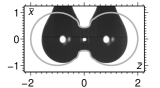
(b) $\bar{t}=0.1$

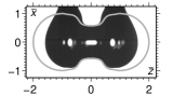
(c) $\bar{t}=0.2$

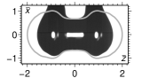
(d) $\bar{t}=0.3$

Figure 1: A typical coalescence event comparing our computations, with free spheres, against experiments in paulsen12 conducted using 1cP pendent drops of silicone oil (1 unit of length is $R=1.1$ mm and 1 unit of time is $T_{i}=8$ ms).

Due to recent advances in both experimental and computational techniques, there has been a surge in the number of publications studying the coalescence of liquid drops in an ambient gas (air) menchacarocha01 ; thoroddsen05 ; wu04 ; aarts05 ; paulsen11 ; fezzaa08 . The experimental aspects of the problem have been driven by the application of both ultra high-speed imaging techniques thoroddsen05 and a novel electrical method paulsen11 , which has circumvented fundamental issues with optical measurements. From a computational perspective, specially-designed codes have been used to capture all scales in the problem and to resolve a flow which is known to be singular sprittles_pof2 ; paulsen12 . Notably, most of the aforementioned works have focussed on the different ‘regimes’ encountered and the ‘transitions’ between them, typically shown on log-log plots, with the main attention to formulating or using the correct ‘scalings’ in each regime.

It has now been established that the crossover from the ‘viscous’, or ‘inertially-limited viscous’ paulsen12 , regime to an ‘inertial regime’, in which viscous forces are negligible compared to inertial ones, occurs when the dimensional radius $r_{b}$ of the bridge (Figure 2) connecting the coalescing drops in the early stages of the process satisfies $\bar{r}_{b}=r_{b}/R\sim\textrm{Re}_{i}^{-1}$ paulsen11 ; sprittles_pof2 , where $\textrm{Re}_{i}=\sqrt{\rho\sigma R/\mu^{2}}$ is the Reynolds number in the inertial regime for a drop of radius $R$, density $\rho$, surface tension $\sigma$ and viscosity $\mu$. This Reynolds number is related to the Ohnesorge number Oh sometimes used in coalescence studies via $\textrm{Oh}=\textrm{Re}_{i}^{-1}$.

Consider now the bridge radius at which water drops will enter the inertial regime. If the drops are millimetre-sized $R=1$ mm, as is often the case in experiments, we have $\textrm{Re}_{i}=O(10^{2})$ so that the drops enter the inertial regime when $r_{b}/R=O(10^{-2})$. If instead microdrops are considered with, say, $R=10~{}\mu$m, then $\textrm{Re}_{i}=O(10)$ and the bridge radius still needs only to reach $r_{b}/R=O(10^{-1})$ before the inertial regime is entered. In other words, for low-viscosity liquids like water the majority of the dynamics of the bridge (defined, crudely, as $r_{b}/R>0.1$) of the coalescence event occurs in the inertial regime, even for the drops encountered in microfluidics. This is the regime which will be considered in this paper.

The inertial regime has previously been studied experimentally, using ultra high-speed cameras menchacarocha01 ; thoroddsen05 ; wu04 ; aarts05 ; paulsen12 ; analytically, by developing scaling laws eggers99 and asymptotic theory thompson12 ; and computationally, considering either the local problem duchemin03 , where the initial stages of bridge front propagation are studied independently from the overall flow configuration, or the global dynamics of the drops menchacarocha01 ; baroudi14 , where the entire geometry is accounted for. It has been shown theoretically eggers99 , computationally duchemin03 ; paulsen12 ; sprittles_pof2 and experimentally menchacarocha01 ; thoroddsen05 ; wu04 ; aarts05 ; paulsen12 that, in this regime, the bridge front propagates with a square root in time scaling. In particular, in eggers99 , the driving capillary pressure $\sigma\kappa$ due to the surface tension and based on the longitudinal curvature $\kappa\sim 1/d(t)$ obtained from the undisturbed free-surface shape of the drops $d(t)\sim r_{b}^{2}(t)/R$ is balanced by the dynamic pressure $\rho\left(dr_{b}/dt\right)^{2}$. As a result, one has $r_{b}/R=C_{i}\left(t/T_{i}\right)^{1/2}$, where $C_{i}$ is a constant of proportionality, so that, once non-dimensionalised by our characteristic scales in this regime, that is $R$ for length and $T_{i}=\sqrt{\rho R^{3}/\sigma}$ for time, the scaling law takes the form

$$\bar{r}_{b}=C_{i}\bar{t}^{1/2}.$$ (1)

Here, and henceforth, all quantities with a ‘bar’ are dimensionless.

Our approach here will be to establish the existence of a well-defined inertial regime, to study the accuracy of scaling laws in this regime using the corresponding numerical solution of the full-scale mathematical problem and to compare their predictions to experimental data from the literature. This will lead us to an improved scaling law for the regime that will be shown to describe experimental data for a much larger period of time than (1) and will allow us to identify previous works where the wrong value of $C_{i}$ in (1) has been chosen.

II Problem formulation

In this work we will consider both the typical experimental setup in which hemispherical drops are grown from syringes as well as the case of most practical interest, where free spheres coalesce (Figure 2). Assuming that gravity can be ignored, which is reasonable for mm-sized drops and below (sprittles_pof2, ) the problem becomes symmetric and can be reduced to determining the motion of one drop in the $(\bar{r},\bar{z})$-plane of a cylindrical coordinate system with the symmetry conditions on the $\bar{z}=0$ plane at which the drops initially touch. The syringe, when considered, is taken to be a semi-infinite cylinder with zero-thickness walls located at $\bar{r}=1,\bar{z}>1$. The precise far field conditions, i.e. those associated with the syringe head, have a negligible effect on the initial stages of coalescence (sprittles_pof2, ).

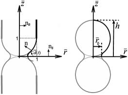
Figure 2: A definition sketch for the coalescence of two identical ‘pinned hemispheres’ grown from syringes (left) and a sketch of coalescing ‘free spheres’ (right) showing the bridge radius $\bar{r}_{b}$ and apex height $h$.

To non-dimensionalise the system of the governing equations for the bulk variables, we use the drop radius $R$ as the characteristic length scale, $U_{i}=\sqrt{\sigma/(\rho R)}$ as the scale for velocities, $T_{i}=\sqrt{\rho R^{3}/\sigma}$ as the time scale and $\mu U_{i}/R$ as the scale for pressure. Then, the continuity and momentum balance equations take the form

$$\nabla\cdot\mathbf{u}=0,\qquad\textrm{Re}_{i}~{}\left[\dfrac{\partial\mathbf{u}}{\partial{t}}+\mathbf{u}\cdot\nabla\mathbf{u}\right]=\nabla\cdot\mathbf{P};$$ (2)

$$\mathbf{P}=-p\mathbf{I}+\left[\nabla\mathbf{u}+\left(\nabla\mathbf{u}\right)^{T}\right],$$

where $\mathbf{P}$, $\mathbf{u}$ and $p$ are the (dimensionless) stress tensor, velocity and pressure in the fluid; $\mathbf{I}$ is the metric tensor of the coordinate system. The Reynolds number is $\textrm{Re}_{i}=\sqrt{\rho\sigma R/\mu^{2}}$.

The conventional boundary conditions used for free-surface flows are the kinematic condition, stating that the fluid particles forming the free surface stay on the free surface at all time and the balance of tangential and normal forces acting on an element of the free surface from the two bulk phases and from the neighbouring surface elements:

$$\dfrac{\partial f}{\partial{\bar{t}}}+\mathbf{u}\cdot\nabla f=0$$ (3)

$$\mathbf{n}\cdot\mathbf{P}\cdot\left(\mathbf{I}-\mathbf{n}\mathbf{n}\right)=\mathbf{0},\qquad\mathbf{n}\cdot\mathbf{P}\cdot\mathbf{n}=\textrm{Re}_{i}\nabla\cdot\mathbf{n}.$$ (4)

Here $f(\bar{r},\bar{z},\bar{t})=0$ describes the a priori unknown free-surface shape, with the unit normal vector $\mathbf{n}=\nabla f/|\nabla f|$ pointing into the liquid, and the tensor $(\mathbf{I}-\mathbf{n}\mathbf{n})$ extracts the component of a vector parallel to the surface with the normal $\mathbf{n}$.

At the plane of symmetry $\bar{z}=0$, the standard symmetry conditions of impermeability and zero tangential stress are applied

$$\mathbf{u}\cdot\mathbf{n}_{s}=0,\qquad\mathbf{n}_{s}\cdot\mathbf{P}\cdot\left(\mathbf{I}-\mathbf{n}_{s}\mathbf{n}_{s}\right)=\mathbf{0},$$ (5)

where $\mathbf{n}_{s}$ is the unit normal to the plane of symmetry. In the conventional model we are studying here, the free surface is assumed to always be smooth so that where it meets the plane of symmetry we have $\mathbf{n}\cdot\mathbf{n}_{s}=0$.

On the axis of symmetry $\bar{r}=0$, the standard normal and tangential velocity condition state that the velocity has only the component parallel to the $\bar{z}$-axis and the radial derivative of this component is zero (the velocity field is smooth at the axis),

$$\mathbf{u}\cdot\mathbf{n}_{a}=0,\quad\frac{\partial}{\partial\bar{r}}[\mathbf{u}\cdot(\mathbf{I}-\mathbf{n}_{a}\mathbf{n}_{a})]=0,\qquad \bar{r}=0;$$ (6)

where $\mathbf{n}_{a}$ is the unit normal to the axis of symmetry in the $(\bar{r},\bar{z})$-plane.

For the case of coalescing free spheres, the free surface is assumed smooth at the apex $\bar{r}=0,\bar{z}=h(\bar{t})$ so that $\mathbf{n}\cdot\mathbf{n}_{a}=0$ there, whilst the case of coalescing pinned hemispheres requires more conditions to account for the presence of the syringe. Specifically, at the point in the $(\bar{r},\bar{z})$-plane where the (initially hemispherical) free surface meets the syringe tip, we have a pinned contact-line:

$$f(1,1,\bar{t})=0\qquad(\bar{t}\geq 0).$$ (7)

It is assumed that in the far field, the liquid inside the syringe are at rest, so that

$$\mathbf{u}\rightarrow\mathbf{0}\qquad\hbox{as}\qquad\bar{r}^{2}+\bar{z}^{2}\rightarrow\infty,$$ (8)

whilst on the cylinder’s surface, no-slip is applied

$$\mathbf{u}=\mathbf{0}\qquad\hbox{at}\qquad\bar{r}=1,\bar{z}\geq 1.$$ (9)

Computations are started from a finite initial bridge radius $\bar{r}_{min}$, and the details of the initial conditions can be very important when considering the initial stages of motion sprittles_pof2 . However, when considering the global motion of the drops, so long as $\bar{r}_{min}$ is sufficiently small, say $\bar{r}_{min}<10^{-2}$, the subtleties surrounding the implementation of the initial conditions are unimportant. Our computations are started from $\bar{r}_{min}=10^{-4}$ and as an initial condition for the free-surface we take a shape which provides a smooth free-surface at $\bar{r}=\bar{r}_{min}$ (which a truncated sphere would not) whilst far away from the origin (i.e. from the point of the initial contact) it is initially the undisturbed hemispherical/spherical drop. A shape which satisfies these criteria can be taken from hopper84 , i.e. the analytic two-dimensional solution to the problem for Stokes flow. In parametric form, the initial free-surface shape is taken to be

$$\bar{r}(\theta) = \sqrt{2}(1+m)H\cos\theta,$$

$$\bar{z}(\theta) = \sqrt{2}(1-m)H\sin\theta,$$ (10)

$$H = \left[(1-m^{2})(1+m^{2})^{-1/2}(1+2m\cos\left(2\theta\right)+m^{2})^{-1}\right]$$

for $0<\theta<\theta_{u}$, where $m$ is chosen such that $\bar{r}(0)=\bar{r}_{min}$ is the initial bridge radius, which we choose, and $\theta_{u}$ is chosen such that $\bar{r}(\theta_{u})=\bar{z}(\theta_{u})=1$ for hemispherical drops and $\bar{r}(\theta_{u})=0$ for spherical ones. Notably, for $\bar{r}_{min}\to 0$ we have $m\to 1$ and $\bar{r}^{2}+(\bar{z}-1)^{2}=1$, i.e. the drop’s profile is a semicircle of unit radius which touches the plane of symmetry at the origin as required.

Finally, we assume that the fluid starts from rest:

$$\mathbf{u}=\mathbf{0}\qquad\hbox{at}\qquad\bar{t}=0.$$ (11)

III Computational approach

The coalescence phenomenon requires the solution of a free-boundary problem with effects of viscosity, inertia and capillarity all present, so that a computational approach is unavoidable. To do so, we use a finite-element framework which was originally developed for dynamic wetting flows and has been thoroughly tested in sprittles_ijnmf ; sprittles_jcp as well as being applied to flows undergoing high free-surface deformation in sprittles_pof , namely microdrop impact onto and spreading over a solid surface. Notably, the method implemented in our computational platform has been specifically designed for multiscale flows, so that the very small length scales associated with the early stages of coalescence can be captured alongside the global dynamics of the two drops’ behaviour. In other words, all of the spatio-temporal scales present in electrical measurements (paulsen11, ), as well as the scales associated with later stages of the drop’s evolution, which are of interest here, can, for the first time, be simultaneously resolved. A user-friendly step-by-step guide to the implementation of the method can be found in (sprittles_ijnmf, ; sprittles_jcp, ) whilst benchmark coalescence simulations are provided in sprittles_pof2 .

IV Results

IV.1 Identifying an inertial regime

In Figure 3, our computed solutions show that for $\textrm{Re}_{i}\geq 10^{2}$ (curves 2, 3a and 3b), the evolution of the bridge between the drops becomes insensitive to further increase in the Reynolds number until the dimensionless radius of the bridge $\bar{r}_{b}\approx 0.75$. Deviations for very small bridge radii $\bar{r}_{b}<\textrm{Re}_{i}^{-1}\leq 10^{-2}$, caused by viscous forces being non-negligible and usually observed on a log-log plot, will not be important in the regime we are focusing on. In this regime hemispheres pinned to the rim of the syringe needles and free spheres (curves 3a and 3b, respectively) give the same results . This suggests that we are truly in an ‘inertial regime’ in which (a) the effects of viscosity are negligible and (b) the process can be considered as ‘local’, i.e. independent of the far-field geometry. It is in this regime that scaling law (1) is expected to approximate the exact solution and has often been used to interpret experimental data (wu04, ; aarts05, ; paulsen11, ).

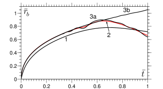
Figure 3: (Color online) Identification of the ‘inertial regime’ showing that above a critical Reynolds number, there is a period in which the bridge’s evolution is independent of the value of $\textrm{Re}_{i}$ or of the flow configuration. Pinned hemispheres are used in computations for 1: $\textrm{Re}_{i}=10$, 2: $\textrm{Re}_{i}=10^{2}$ (in red), 3a: $\textrm{Re}_{i}=10^{3}$, whilst curve 3b is for free sphere with $\textrm{Re}_{i}=10^{3}$.

IV.2 Standard scalings

In Figure 4, we can see that scaling law (1) with $C_{i}=1.5$ (curve 1) provides a good approximation of the computed solution (solid line) for $\bar{r}_{b}<0.15$. However, the scaling law quickly begins to overshoot the numerical solution. Worryingly, most comparisons between this scaling law and experimental data has been in the range accessible to optical observation $\bar{r}_{b}>0.1$ (which for a millimetre-sized drop is $r_{b}=100$ $\mu m$) where our computations show that the scaling law greatly overshoots the computed solution. In other words, it has been used outside the region where it gives a reasonable approximation of the solution of the mathematical problem it is supposed to mimic.

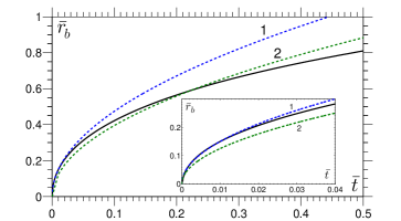
Figure 4: (Color online) Comparison of the computed solution (solid line) to equation (1) with $C_{i}=1.5$ (curve 1 in blue) and $C_{i}=1.25$ (curve 2 in green).

If instead we had looked to ‘fit’ the whole of the computed curve in the region $0.1<\bar{r}_{b}<0.75$ as best as we can, ignoring large errors for $\bar{r}_{b}<0.1$, then the result is that the prefactor must have a much smaller value of $C_{i}=1.25$ (curve 2 in Figure 4) the value which is closer to those obtained in previous experimental works (aarts05, ; wu04, ) that fitted (1).

The upshot of the discrepancy between the scaling law and the computed solution in the experimental range is that reported values of $C_{i}$ have been too small. Although a value of $C_{i}=1.25$, consistent with those obtained from experimental analysis aarts05 ; wu04 , provides a ‘best fit’ (curve 2 in Figure 4) for $0.1<\bar{r}_{b}<0.75$ to the exact solution (solid line), and hence also to the experimental data (Figure 6), as can be seen from Figure 4 this solution completely fails to capture the correct behaviour as $\bar{r}_{b}\to 0$, where the scaling law should asymptotically approach the exact solution (solid curve).

The failure of the ‘best fit’ approach is confirmed in Figure 5, where the relative percentage error $E_{b}(\bar{t})=100|\bar{r}_{sc}-\bar{r}_{co}|/\bar{r}_{co}$ of the scaling laws $\bar{r}_{b}=\bar{r}_{sc}(\bar{t})$ from the computed solution $\bar{r}_{b}=\bar{r}_{co}(\bar{t})$ is plotted as a function of time. One can see that the scaling law (1) with $C_{i}=1.5$ approximates the computed solution well, with $E_{b}<3\%$ for $\bar{t}<2\times 10^{-2}$ whilst during the same time period $E_{b}>15\%$ for curve 2 which is the ‘best fit’ attempt $C_{i}=1.25$ in (1). The error also confirms that whilst (1) with $C_{i}=1.5$ captures the correct behaviour in the inertial regime for small times, this solution rapidly departs from the computed solution, with $E_{b}>12\%$ for $\bar{t}>0.1$. If, as a crude estimate, we require a scaling law to satisfy $E_{b}<5\%$, then we see that curve 1 meets this criterion for $\bar{t}<0.03$ whilst curve 2 fails in the initial stages and is only valid for $0.12<\bar{t}<0.36$. Thus, neither of the current scaling laws provide satisfactory approximations to the computed solutions which could be used for a quick comparison between experimental and theoretical predictions.

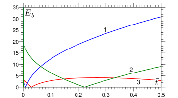
Figure 5: (Color online) The relative percentage error $E_{b}$ of the scaling laws from the computed solution. Curve 1 (in blue) is for (1) with $C_{i}=1.5$, curve 2 (in green) is (1) taking $C_{i}=1.25$ and curve 3 (in red) is (15) with $C_{i}=1.5$.

Here, we will look to rectify the aforementioned inconsistencies by extending the scaling law (1), using the approach initiated in thoroddsen05 , to account for the azimuthal curvature, which reduces the capillary pressure and hence acts to slow down the evolution of the bridge, as well as the longitudinal curvature that drives the process. Although, as we shall see, the latter dominates as $\bar{r}_{b}\to 0$, it is anticipated that, by including the azimuthal curvature in the scaling law, we will be able to increase the region of applicability of our scaling to within the optical range. This should give a more accurate representation of the bridge evolution in the inertial regime and can be used to predict the speed of coalescence without having to resort to computations.

IV.3 An improved scaling

Including the curvature at the bridge front in the azimuthal direction, i.e. $\bar{\kappa}_{2}=-1/\bar{r}_{b}$, which acts to resist the bridge’s outward motion, into our expression for the full curvature $\bar{\kappa}$ is simple; however, as a consequence of this extension, we must specify how the longitudinal curvature $\bar{\kappa}_{1}$ scales as the bridge propagates since we are no longer able to ‘absorb’ this scale into the constant of proportionality. Thus, we now have

$$\bar{\kappa}=\bar{\kappa}_{1}+\bar{\kappa}_{2}=\frac{A}{\bar{r}_{b}^{2}}-\frac{1}{\bar{r}_{b}}$$ (12)

where the constant $A$ must be specified to account for the longitudinal curvature behaviour as the bridge expands. Previously, i.e. in (1), the second term on the right-hand side was neglected and this constant was simply absorbed into $C_{i}$. If the undisturbed free surface height at $\bar{r}_{b}$ is taken as the radius of curvature at that point, then, for small $\bar{r}_{b}$, we have $A=2$. However, in thoroddsen05 , it is argued that $A\approx 1$ gives a better agreement with experiments as with this value the radius of curvature is the distance between the two undisturbed free surfaces rather than the distance from the plane of symmetry to one of them and hence accounts for the “bulb which develops at the end of the advancing interface”. This assertion is confirmed by our computations shown in Appendix and so, henceforth, we assume $A=1$ and, if needs be, can later consider whether more accurate representations of $A$ are required. In thoroddsen05 , the resulting equations, which considered drops of different sizes, were solved using a numerical method and seen to give good agreement with the experimental data.

In the case of the coalescence of two identical liquid drops, with curvature given by (12), it will be shown that an analytic solution can be obtained which, now $A$ has been specified, still contains only one free constant. As proposed in eggers99 , balancing (dimensionless) inertial forces with the (driving) surface tension force gives

$$\left(\dfrac{\mathrm{d}\bar{r}_{b}}{\mathrm{d}{\bar{t}}}\right)^{2}=\frac{C_{i}^{4}}{4}\left(\frac{1}{\bar{r}_{b}^{2}}-\frac{1}{\bar{r}_{b}}\right).$$ (13)

where the coefficient of proportionality has been chosen so that if the azimuthal curvature is ignored, we recover $\bar{r}_{b}=C_{i}\bar{t}^{1/2}$. Integrating (13), assuming that $\bar{r}_{b}=0$ at $\bar{t}=0$ , and rearranging we obtain a cubic polynomial in $\bar{r}_{b}$ with $\bar{t}$ as a parameter:

$$\bar{r}_{b}^{3}+3\bar{r}_{b}^{2}+\frac{3C_{i}^{2}\bar{t}}{4}\left(\frac{3C_{i}^{2}\bar{t}}{4}-4\right)=0.$$ (14)

We can see immediately that if only the leading order terms in $\bar{r}_{b}$ and $\bar{t}$ are kept, we have $3\bar{r}_{b}^{2}-3C_{i}^{2}\bar{t}=0$ so that the usual scaling (1) is recovered. The solution which we require is given by

$$\bar{r}_{b}=\frac{s}{4}+\frac{4}{s}-1,\qquad s=\left[-64-18d^{2}+96d+2\left(2880d^{2}\right.\right.$$

$$\left.\left.-3072d+81d^{4}-864d^{3}\right)^{1/2}\right]^{1/3},\qquad d=C_{i}^{2}\bar{t},$$ (15)

where we take the root with the positive imaginary part for $s$ , which results in $\bar{r}_{b}$ being real.

IV.4 Comparison of the improved scaling law to simulations and experiments

The explicit form of (15) allows for quick comparison with computed solution or experiments, with no additional fitting parameters, in order to determine whether this is a significant improvement on (1). In the subplot of Figure 6, it can be clearly seen that for the same value of $C_{i}=1.5$, the new scaling law (curve 2) gives results indistinguishable from those given by (1) (curve 1) for $\bar{r}_{b}<0.15$ but for $0.15<\bar{r}_{b}<0.8$ (shown in the main plot), i.e. for the range usually used in experimental works to fit a scaling law to the data, the new expression agrees far better with the simulation of the full system (solid line computed for free-spheres) than the expression (1). This is confirmed in Figure 5 where it can be seen that the new scaling law is within 5% of the computed solution at least up to $\bar{t}=0.5$. Although curve 2 is not indistinguishable from the numerical result for $\bar{r}_{b}>0.4$ in Figure 6, as one may expect from the simplifications made, as an approximating formula it is a significant improvement on the previous result and is close to the numerical solution for a remarkably large proportion of the coalescence process.

In Figure 6, it can be clearly seen that the new ‘universal curve’ (curve 2) is able to capture experimental data for the inertial regime collected from the literature completely different geometric configurations (hanging pendent drops, pinned hemispheres and spheres supported by a hydrophobic solid) and thus provides the sought-after extension to (1) required to approximate the coalescence dynamics in this regime whilst retaining a simple analytic expression.

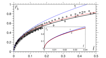
Figure 6: (Color online) Comparison of the computed solution (solid black curve) of free spheres coalescing with $\textrm{Re}_{i}=10^{3}$ to equation (1) with $C_{i}=1.5$ (curve 1 in blue) and the new scaling (15) also with $C_{i}=1.5$ (curve 2 in red). Data has been obtained from the lowest viscosity drops considered in the following publications: circles, Figure 3F in paulsen12 ; squares, Figure 6 in thoroddsen05 ; triangles, Figure 3a in aarts05 ; diamonds, Figure 6 in menchacarocha01 ; and stars, best-fit to Figure 4 in wu04 .

In Figure 1, we can see that the initial dynamics of coalescence in the inertial regime is genuinely ‘local’, as the two different geometries used for experiments (pendent drops) and simulations (free spheres) agree for the initial stages of motion, i.e. the deformed free surface in both the experiment and the simulation agree perfectly even though their entire shapes, by construction, do not. It is only around $\bar{t}=0.3$ that the free surface shapes in the bridge region start to feel their entire geometry, so that the inertial regime is essentially over as the bridge’s propagation is no longer ‘local’. Despite this, it is seen from Figure 6 that the estimates for the bridge radius stay close to the exact solution and the experimental data for a considerably longer time, remaining relatively accurate until at least $\bar{t}=0.5$ at which point $\bar{r}_{b}\approx 0.8$.

A shortcoming of the obtained expression is that it does not include the influence of gravity on the drops’ evolution, which manifests itself most strongly by altering the initial shape of drops. This effect will be significant for drops larger than the capillary length, which for water is of the order of millimetres. However, for smaller low-viscosity drops, particularly those from around $R=10$ $\mu m$ to $R=1$ mm, where inertial effects still dominate viscous ones, the expression in (15) will provide an excellent approximation to their evolution.

Appendix: Computation of the longitudinal curvature

Figure 8 shows the free surface shape obtained from the computed solution for free spheres coalescing at $\textrm{Re}_{i}=10^{3}$ in the range $0.1\leq\bar{r}_{b}\leq 0.7$. Marked with crosses are the point on the free surface at which the longitudinal curvature $\bar{\kappa}_{1}$ changes sign, i.e. the crosses mark an inflection point in the free-surface profile. The height of this inflection point $\bar{z}=\bar{z}_{inf}$ can be used to define the effective longitudinal curvature of the bridge connecting the coalescing drops as $\bar{\kappa}_{1}=1/\bar{z}_{inf}$. This allows us to test the assumption that $\bar{\kappa}_{1}\approx 1/\bar{r}_{b}^{2}$, or alternatively that $\bar{\kappa}_{1}\bar{r}_{b}^{2}\approx 1$.

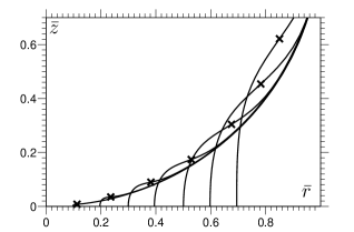
Figure 7: Snapshots of the coalescence process showing crosses at the inflection point on the free surface.

In Figure 8, it can be seen that in the range $0.1\leq\bar{r}_{b}\leq 0.7$ we have $\kappa_{1}\bar{r}_{b}^{2}$ approximately constant, so that the assumed scaling behaviour sufficiently accurately reflects the exact solution: over the period considered it is in the range $\kappa_{1}\bar{r}_{b}^{2}\in(0.8,1.2)$ so that its average value will be close to one. Slight improvements could potentially be achieved by using a linear approximation for the curvature, but given the good agreement between the new scaling and the fully computed results this does not seem necessary.

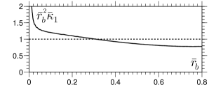
Figure 8: Evolution of the computed effective longitudinal curvature of the bridge connecting the coalescing drops $\bar{\kappa}_{1}$ multiplied by the square of the bridge radius $\bar{r}_{b}^{2}$. It can be seen that $\bar{\kappa}_{1}\bar{r}_{b}^{2}\approx 1$ as assumed.

References

- [1] J. D. Paulsen, J. C. Burton, S. R. Nagel, S. Appathurai, M. T. Harris, and O. Basaran. The inexorable resistance of inertia determines the initial regime of drop coalescence. Proceedings of the National Academy of Science, 109:6857–6861, 2012.
- [2] A. Menchaca-Rocha, A. Martínez-Dávalos, R. Núńez, S. Popinet, and S. Zaleski. Coalescence of liquid drops by surface tension. Physical Review E, 63:046309, 2001.
- [3] S. T. Thoroddsen, K. Takehara, and T. G. Etoh. The coalescence speed of a pendent and sessile drop. Journal of Fluid Mechanics, 527:85–114, 2005.
- [4] M. Wu, T. Cubaud, and C. Ho. Scaling law in liquid drop coalescence driven by surface tension. Physics of Fluids, 16:51–54, 2004.
- [5] D. G. A. L. Aarts, H. N. W. Lekkerkerker, H. Guo, G. H. Wegdam, and D. Bonn. Hydrodynamics of droplet coalescence. Physical Review Letters, 95:164503, 2005.
- [6] J. D. Paulsen, J. C. Burton, and S. R. Nagel. Viscous to inertial crossover in liquid drop coalescence. Physical Review Letters, 106:114501, 2011.
- [7] K. Fezzaa and Y. Wang. Ultrafast x-ray phase-contrast imaging of the initial coalescence phase of two water droplets. Physical Review Letters, 100:104501, 2008.
- [8] J. E. Sprittles and Y. D. Shikhmurzaev. Coalescence of liquid drops: Different models versus experiment. Physics of Fluids, 24:122105, 2012.
- [9] J. Eggers, J. R. Lister, and H. A. Stone. Coalescence of liquid drops. Journal of Fluid Mechanics, 401:293–310, 1999.
- [10] A. B. Thompson and J. Billingham. Inviscid coalescence in the presence of a surrounding fluid. IMA Journal of Applied Mathematics, 77:678–696, 2012.
- [11] L. Duchemin, J. Eggers, and C. Josserand. Inviscid coalescence of drops. Journal of Fluid Mechanics, 487:167–178, 2003.
- [12] L. Baroudi, M. Kawaji, and T. Lee. Effects of initial conditions on the simulation of inertial coalescence of two drops. Computers and Mathematics with Applications, 67:282–289, 2014.
- [13] R. W. Hopper. Coalescence of two equal cylinders: exact results for creeping viscous plane flow driven by capillarity. Journal of the American Ceramic Society, 67:262–264, 1984.
- [14] J. E. Sprittles and Y. D. Shikhmurzaev. A finite element framework for describing dynamic wetting phenomena. International Journal for Numerical Methods in Fluids, 68:1257–1298, 2012.
- [15] J. E. Sprittles and Y. D. Shikhmurzaev. Finite element simulation of dynamic wetting flows as an interface formation process. Journal of Computational Physics, 233:34–65, 2013.
- [16] J. E. Sprittles and Y. D. Shikhmurzaev. The dynamics of liquid drops and their interaction with solids of varying wettabilities. Physics of Fluids, 24:082001, 2012.
- [17] It is the capillary waves, initiated at the onset of coalescence, travelling along the free surface and interacting with the far field boundary that eventually ‘kill’ the local nature of the solution in this regime.
- [18] A finite radius of contact could easily be added, but experiments demonstrate that this radius is very small, so that its inclusion would have almost no effect on the resulting evolution in the regime of interest.
- [19] This is the default root for most software, e.g. MATLAB.