Mechanical Properties and Plasticity of a Model Glass Loaded Under Stress Control

Abstract

Much of the progress achieved in understanding plasticity and failure in amorphous solids had been achieved using experiments and simulations in which the materials were loaded using strain control. There is paucity of results under stress control. Here we present a new method that was carefully geared to allow loading under stress control either at $T=0$ or at any other temperature, using Monte-Carlo techniques. The method is applied to a model perfect crystalline solid, to a crystalline solid contaminated with topological defects, and to a generic glass. The highest yield stress belongs to the crystal, the lowest to the crystal with a few defects, with the glass in between. Although the glass is more disordered than the crystal with a few defects, it yields stress is much higher than that of the latter. We explain this fact by considering the actual microscopic interactions that are typical to glass forming materials, pointing out the reasons for the higher cohesive nature of the glass. The main conclusion of this paper is that the instabilities encountered in stress-control condition are the identical saddle-node bifurcation seen in strain-control. Accordingly one can use the latter condition to infer about the former. Finally we discuss temperature effects and comment on the time needed to see a stress controlled material failure.

I Introduction

Plasticity in crystalline solids is known to be carried by defects, typically dislocations, that glide irreversibly under the influence of loading the material with some mechanical load MS73 ; C53 . On the other hand, the study of plasticity and yield in amorphous solids is an ongoing subject of research, with many issues remaining to be discovered, especially in more complex amorphous glasses like polymeric glasses and metallic glasses. Much of the recent progress in understanding plasticity in amorphous solids was based on experiments and simulations done by loading the system under strain control protocols. A useful simulational protocol that attracted much attention is the quasi-static athermal (AQS) strain control protocol, in which the system is maintained at zero temperature, and is allowed to return to mechanical equilibrium after every small increase in strain ML04 ; KLLP10 . This protocol exposed very nicely the role of mechanical instabilities. These are easily detected by examining the Hessian matrix of the system; the eigenvalues of this matrix are all positive when the system is mechanically stable, while a plastic instability is characterized by an eigenvalue approaching zero, typically via a saddle-node bifurcation 98ML . When this happens, the associated eigenfunction, which is also identified with the non-affine response of the system, localizes on a sub-set of particles, those that participate in the plastic event.

In this paper we examine the corresponding physics for stress controlled protocols. In some sense, this is the more natural protocol because it provides one with the right control to precisely determine when does the system yield in the sense that its strain will increase indefinitely as long as the stress is maintained at a given value. When the stress is below the yield stress $\sigma_{{}_{\rm Y}}$ the strain will reach a limit. Indeed, some attempts to study yield using stress controlled simulations were reported in the literature FL98 ; RS09 . We propose a more straightforward protocol that appears to provide highly stable results which are in good correspondence with the best available strain-controlled results. The new protocol is introduced in Sect. II. In Sect. III we present the physical models employed here. We discuss stress-controlled loading of a perfect hexagonal structure in 2-dimensions, the same structure marred by some defects, and finally a generic binary glass. This section includes some of the main conclusions of this study: we argue that the instabilities seen in stress control loading are the very same saddle-node bifurcations that are exhibited in strain-controlled experiments. The difference is that once the system yields in stress-control there is no recovery. In strain controlled loading the system can yield, release a portion of its stress, and then be loaded again, to yield again etc. Therefore one sees the typical serrated stress vs. strain curves that can go for some time up to high values of the strain. In contrast, in stress controlled experiments the system either gets stuck if the applied stress is smaller than the yield stress, or it fails if the stress is higher than the yield stress. We show that the knowledge of strain controlled results is useful in predicting much of what can happen in stress controlled loading. In Sect. IV we focus on thermal effects, and particularly what happens when the stress is lower than the yield stress but temperature fluctuations can result in surmounting the barrier and failing. Predicting the waiting time becomes an easy exercise once one realizes that the transition is due to a saddle node bifurcation. This fact implies that the eigenvalue that vanishes at the transition has a square-root singularity, and together with the generic dependence of the barrier hight on the distance from the bifurcation one can easily estimate the waiting time. Sect. V offers a summary and some concluding remarks.

II Statistical mechanics of loaded systems

In this section we construct a protocol based on a method that was proposed for the simulations of deformations in solids in Ref. PR80 . The main ingredient in this approach is in changing the shape of the simulation box as well as its size. In principle this approach can be adapted to either molecular dynamics or Monte Carlo techniques as can be see in e.g. Refs. PR80 ; PR81 ; WTK03 ). This method can be used even for large deformations under applied external forces, see Refs. RR84 ; LB94 .

In the variable shape method PR80 ; PR81 the particle positions change from the reference state $\{{\bm{r}}^{0}_{i}\}$ to a new one, denoted $\{{\bm{r}}_{i}\}$, by an affine transformation that is defined by a matrix ${\bf J}$ :

$${\bm{r}}_{i}={\bm{J}}\cdot{\bm{r}}_{i}^{0}.$$ (1)

On the microscopic level the affine transformation Eq. (1) destroys mechanical equilibrium, and it should be followed by a non-affine atomic-scale relaxation of the particle positions $\{{\bm{r}}^{0}_{i}\}$ LM06 . This relaxation can be performed by Molecular Dynamics or Monte Carlo methods or in the case of a athermal system by energy minimization.

In the frame of statistical mechanics the mean value of an observable in a loaded system is defined by

$$\langle A\rangle=\frac{\int{\rm d}{\bm{J}}{\rm d}{\bm{r}}_{1}^{0}\cdots{\rm d}{\bm{r}}_{N}^{0}~{}A({\bm{r}}_{i}^{0},{\bm{J}})\cdot e^{-G(\{{\bm{r}}_{i}^{0}\},{\bm{J}},{\bm{\sigma}}^{ext})/T}}{\int\mathrm{d}{\bm{J}}\cdot{\bm{r}}_{1}^{0}\cdots{\rm d}{\bm{r}}_{N}^{0}\cdot e^{-G(\{{\bm{r}}_{i}^{0}\},{\bm{J}},{\bm{\sigma}}^{ext})/T}},$$ (2)

Here $T$ is the temperature and $G(\{\bf r_{i}^{0}\},{\bm{J}},{\bm{\sigma}}^{ext})$ is the generalized enthalpy and ${\bm{\sigma}}^{ext}$ is the external stress tensor. The Monte Carlo method allows to evaluate this expression numerically.

The method of variable shape introduces strain into the simulation box by first defining a square box of unit area where the particles are at positions ${\bm{s}}_{i}$. Next one defines a linear transformation ${\bm{h}}$, taking the particles to positions ${\bm{r}}_{i}$ via ${\bm{r}}_{i}={\bf h}\cdot{\bm{s}}_{i}$. In order to prevent rotations of the simulation box, the matrix ${\bf h}$ should be symmetric. The current area of a system becomes the determinant $V=\mid{\bf h}\mid$. Then the positions of the particles in the reference state are defined by ${\bm{r}}^{0}_{i}={\bf h}_{0}\cdot\vec{s}_{i}$; accordingly the matrix ${\bf J}$ in Eq. (1) is given by ${\bf J}={\bf h}\cdot{\bf h}_{0}^{-1}$.

It is suitable to change integrals over the components of the matrix ${\bm{J}}$ in Eq. (2) by integrals over the independent components of the matrix ${\bf h}$ and the integrals over ${\bf r_{i}^{0}}$ by integrals over ${\bf S}=\{\vec{s}_{i}\}$. Then this equation reads

$$\langle A\rangle=\frac{\int\mathrm{d}{\bf h}\cdot\mathrm{d}{\bf S}\cdot\cdot A({\bf S},{\bf h})\cdot e^{-G^{\prime}({\bf S},{\bf h},\bm{\sigma}^{ext})/T}}{\int\mathrm{d}{\bf h}\cdot\mathrm{d}{\bf S}\cdot\cdot e^{-G^{\prime}({\bf S},{\bf h},\bm{\sigma}^{ext})/T}},$$ (3)

where

$$G^{\prime}({\bf S},{\bf h},\bm{\sigma}^{ext})=-TN\ln V+G({\bf S},{\bf h},\bm{\sigma}^{ext}).$$ (4)

The integral in Eq. (3) is evaluated via the Metropolis algorithm. Two kinds of trial moves are considered: one performs $n$ standard Monte Carlo moves (displacement of the particle positions given by $\vec{s}_{i}$)

$${\bm{s}}^{new}_{i}={\bm{s}}^{old}_{i}+\delta{\bm{s}},\hskip 11.38109pt1\leq i\leq N.$$ (5)

In this equation the $\alpha$ component of the displacement vector of a particle is given by

$$\delta s^{\alpha}=\Delta s_{max}(2\xi^{\alpha}-1),$$ (6)

where $\Delta s_{max}$ is the maximum displacement and $\xi^{\alpha}$ is an independent random number uniformly distributed between 0 and 1 After $n$ sweeps defined by Eq. (5) the transformation ${\bf h}$ changes according to

$${\bm{h}}^{new}={\bm{h}}^{old}+\delta{\bm{h}},$$ (7)

where elements of the random symmetric matrix $\delta{\bm{h}}$ are defined by

$$\delta h_{ij}=\Delta h_{max}(2\xi_{ij}-1),\hskip 11.38109pti\leq j.$$ (8)

Here $\Delta h_{max}$ is the maximum allowed change of a matrix element and $\xi_{ij}$ is an independent random number uniformly distributed between 0 and 1. The value of $\Delta h_{max}$ and the maximum displacement of particle positions $\Delta s_{max}$ are selected so that the acceptance rate is $30\%$. For each kind of move the trial configuration is accepted with probability

$$P_{tr}=\min\bigg{[}1,exp\bigg{(}-\frac{\Delta G^{\prime}}{T}\bigg{)}\bigg{]}.$$ (9)

For relaxation of particle positions the matrix ${\bm{h}}$ is fixed and the difference of the generalized enthalpy is defined by the difference of the potential energy of the system $U({\bm{h}},\{{\bm{s}}\})$

$$\Delta G^{\prime} = U({\bm{h}},{\bm{s}}_{1},\cdots,{\bm{s}}_{i}^{new},\cdots{\bm{s}}_{N})-$$ (10)

$$U({\bm{h}},{\bm{s}}_{1},\cdots,{\bm{s}}_{i}^{old},\cdots{\bm{s}}_{N}),\hskip 11.38109pt1\leq i\leq N.$$

The change of the generalized enthalpy due to affine transformation (at fixed particle positions $\{{\bm{s}}\}$) is given by

$$\Delta G^{\prime} = -TN\ln\big{(}V^{new}/V^{old}\big{)}+U({\bm{h}}^{new},\{{\bm{s}}\})$$ (11)

$$- U({\bm{h}}^{old},\{{\bm{s}}\})+\delta W,$$

where $\delta W$ s the work that is done by an external stress ${\bm{\sigma}}^{ext}$. In general case for move ${\bm{J}}\to{\bm{J}}+\delta{\bm{J}}$ this work is given by (see, e.g., WLY95

$$\delta W=-\frac{1}{2}V^{old}Tr\big{(}{\bm{\sigma}}^{ext}(\delta{\bm{J}}{{\bm{J}}}^{-1}+\tilde{{\bm{J}}}^{-1}\delta\tilde{{\bm{J}}})\big{)}.$$ (12)

Here the symbol $\tilde{~}{}$ represents the transpose of a matrix. Taking into account the relation between the matrices ${\bm{J}}$ and ${\bm{h}}$ this equation can be written as

$$\delta W=-\frac{1}{2}Tr\big{(}{\bm{\sigma}}^{ext}(\delta{\bm{h}}{{\bm{H}}}+\tilde{{\bm{H}}}\delta\tilde{{\bm{h}}})\big{)},$$ (13)

where the matrix ${\bm{H}}$ is given by

$${\bm{H}}=\left(\begin{array}[]{cc}h_{yy}&-h_{xy}\\ -h_{xy}&h_{xx}\end{array}\right)$$ (14)

It follows from Eq. (9) that in the limit $T\to 0$ only the configurations with decreasing enthalpy are accepted, i.e., the Monte Carlo process converges to one configuration with minimal generalized enthalpy (for $T=0$ the generalized enthalpy is equal to the Gibbs free energy). In general, this configuration belongs to a local minimum of the generalized enthalpy landscape and its position depends on the initial configuration of the simulation process.

To specialize the technique described above to stress-controlled simple shear simulations at zero temperature one chooses the following ${\bf h}$ matrix

$${\bf h}=L\left(\begin{array}[]{c c}1&\gamma\\ 0&1\end{array}\right),$$ (15)

where $L$ is the length of the square simulation box and $\gamma$ is the simple shear strain, with the volume of the system V=$L^{2}$ being conserved. The external stress in this protocol is given by

$${\bm{\sigma}}=\left(\begin{array}[]{c c}0&\sigma^{ext}_{xy}\\ \sigma^{ext}_{xy}&0\end{array}\right)\ .$$ (16)

For the matrix ${\bm{h}}$ defined by Eq. (15) the change of the generalized enthalpy due to the increment $\delta\gamma$ is given by

$$\Delta G^{\prime}=U({\bm{\gamma}}+{\bm{\delta\gamma}},{\bm{r}}_{i}^{new})-U({\bm{\gamma}},{\bm{r}}_{i}^{old})-V\sigma^{ext}_{xy}\delta\gamma.$$ (17)

Summing Eq. (17) over infinitesimal increments one can find the generalized enthalpy at a given state parameterized by $\gamma$, relative to the state defined by $\gamma_{0}$

$$G^{\prime}(\gamma,\gamma_{0},\sigma^{ext}_{xy})=U({\bm{\gamma}},{\bm{r}}_{i}^{\gamma})-U({\bm{\gamma}}_{0},{\bm{r}}_{i}^{\gamma_{0}})-V\sigma^{ext}_{xy}(\gamma-\gamma_{0}),$$ (18)

where $U({\bm{\gamma}},{\bm{r}}_{i}^{\gamma})$ is the energy that is achieved after a sequence of steps in the frame of this protocol. Usually the reference state corresponding to $\gamma_{0}$ is defined at $\sigma^{ext}_{xy}=0$. Nevertheless, as one can see from Eq. (18) the replacement of the reference state generates only a shift by a constant in the generalized enthalpy; Once the generalized enthalpy is minimized the location of the minima do not depend on the reference state.

Note that the strain $\gamma$ appears explicitly in our formalism. It is therefore important to stress that in general the strain is not a state function if the system undergoes irreversible events during the nonaffine position reshuffling in which energy can be lost to the heat bath 01Gil . The generalized enthalpy is determined by $\gamma$ as a state function only in the case of pure elasticity. Here the appearance of $\gamma$ in the formalism should be interpreted only as a marker to the present shape of the system, and the energy has to be computed incrementally via following the protocol.

In the next section we present the results of MC calculations for the temperature $T=0.05$ and the pressure $P=0$ at different values of applied shear stress. For the sake of more easy interpretation these results are compared with the consequences of the AQS strain-controlled protocol.

III The model and simulation results

A two-dimensional binary mixture consists of two kinds of particles $A$ and $B$. The interatomic interactions are defined by shifted and smoothed Lennard-Jones potentials

$$\phi_{\alpha\beta}(r)=\left\{\begin{array}[]{ll}\phi_{\alpha,\beta}^{LJ}(r)+A_{\alpha\beta}+B_{\alpha\beta}r+C_{\alpha\beta}r^{2}&\textrm{if $r\leq R^{cut}_{\alpha\beta}$,}\\ 0&\textrm{if $r>R^{cut}_{\alpha\beta}$,}\end{array}\right.$$ (19)

where

$$\phi_{\alpha\beta}^{LJ}(r)=4\epsilon_{\alpha\beta}\bigg{[}\bigg{(}\frac{\sigma_{\alpha\beta}}{r}\bigg{)}^{12}-\bigg{(}\frac{\sigma_{\alpha\beta}}{r}\bigg{)}^{6}\bigg{]}.$$ (20)

It is convenient to introduce reduced units, with $\sigma_{AA}$ being the unit of length and $\epsilon_{AA}$ the unit of energy. All the potentials given by Eq. (19) vanish with two zero derivatives at distances $R^{cut}_{\alpha\beta}=2.5\sigma_{\alpha\beta}$. The parameters in Eq. (20) KA94 and in the smoothing part of Eq. (19) are given in Tab. 1. The dependence of the potentials defined by Eq. (19) on the distance between particles is shown in Fig. 1.

Table 1: Potential parameters.

Particles	$\sigma_{\alpha\beta}$	$\epsilon_{\alpha\beta}$	$A_{\alpha\beta}$	$B_{\alpha\beta}$	$C_{\alpha\beta}$
AA	1.00	1.0	0.4527	-0.3100	0.0542
BB	0.88	0.5	0.2263	-0.1762	0.0350
AB	0.80	1.5	0.6790	-0.5814	0.1271

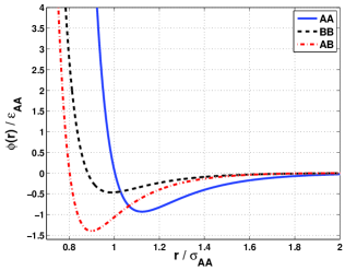
Figure 1: Interaction potentials in dimensionless units.

A composition of $A$ and $B$ particles that is stable in two-dimensions against crystallization is chosen to be $65\%$ of particles $A$ and $35\%$ of particles $B$ BOPK09 . For the one component system that is discussed below the potential of interaction is chosen to be that of particles $A$.

III.1 The perfect hexagonal structure

III.1.1 Finite temperature

As a first step we studied the properties of a one component system consisting of $N=256$ particles with the interaction potential of $A$ particles. A Monte Carlo process with $10^{6}$ sweeps at a chosen value of the shear stress was run using the shape-varying protocol described above. We always begin our simulations from the liquid state, and cool down to a chosen temperature. This process invariably leaves, even for a one component system, some defects in the self-forming crystalline hexagonal solid. In other words, typically one finds, upon cooling, a configuration like the one shown in the lower panel of Fig. 2, denoted as configuration ${\bf II}$). These remaining defects can be removed by straining the system back and forth as was done in Ref. ABHIMPS07 . The resulting perfect hexagonal structure (the configuration ${\bf I}$) obtained in this way is shown in the top panel of Fig. 2.

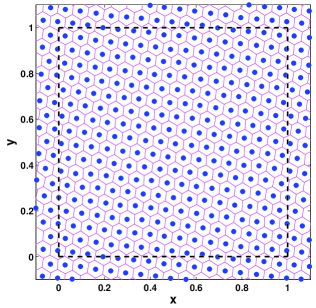
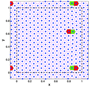
Figure 2: Configurations of the one component system. Top panel - configuration I with perfect hexagonal structure. Bottom panel - configuration II with defects. The dotted line represents the simulation cell which is continued periodically in both directions.

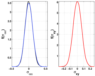
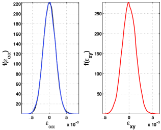
Figure 3: Distributions of the stress tensor components (upper panel) and strain tensor components (bottom panel) of the perfect hexagonal structure at $\bm{\sigma}^{ext}=0$ at temperature $T=0.05$ ($\alpha=x,y$).

The distribution of the components of the internal stress and strain tensors at zero pressure and with the external stress ${\bm{\sigma}}^{ext}=0$ and $T=0.05$ is shown in Fig. 3. The components of the internal stress tensor are defined by

$$\sigma_{\alpha\beta}^{int}=\rho T\delta_{\alpha\beta}-\frac{1}{2V}\sum\limits_{{\bm{K}},{\bm{L}}}\sum\limits_{i\neq j}\frac{\partial\phi_{{\bm{K}}{\bm{L}}}(r_{ij})}{\partial r_{ij}}\frac{r_{ij}^{\alpha}r_{ij}^{\beta}}{r_{ij}},$$ (21)

where $r_{ij}$ is the distance between particles $i$ and $j$, $\alpha,\beta=x,y$ denotes components of a vector ${\bm{r}}_{ij}$ and ${\bm{K}},{\bm{L}}=A,B$ distinguish the kind of a particle. The strain tensor is defined here by

$${\bm{\epsilon}}=\frac{1}{2}\big{(}\tilde{{\bm{h}}_{0}}^{-1}\tilde{{\bm{h}}}{{\bm{h}}}{{\bm{h}}_{0}^{-1}}-{{\bm{I}}}\big{)},$$ (22)

where ${\bm{h}}_{0}=\langle{\bm{h}}\rangle$.

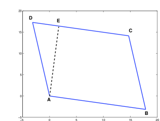
Figure 4: Shape of the simulation box. The segment AE is perpendicular to the side CD

For notational purposes it is more convenient to use a definition of shear deformation instead of Eq. (22). A current shape of the simulation box is shown in Fig. 4. The strain (so-called engineer shear strain) is given by

$$\gamma=\frac{L_{ED}}{L_{AE}},$$ (23)

where $L_{ij}$ is the distance between points $i$ and $j$. The same definition of strain is used in Eq. (15). In order to define the deformation relative to a reference state we will use also the quantity $\gamma_{r}=\gamma-\gamma_{0}$, where $\gamma_{0}=\langle\gamma\rangle_{\sigma^{ext}_{xy}=0}$.

At this point the applied shear stress is increased in steps, and after each increase the Monte Carlo process is run for 10 particles exchange sweeps, followed by a change in the shape ${\bm{h}}$, followed again by 10 particles sweeps and again a shape change, accumulating altogether to $10^{6}$ sweeps. As long as the chosen applied shear stress $\sigma_{xy}^{ext}$ is smaller than $\sigma_{{}_{\rm Y}}\simeq 1.56$ the shear strain $\gamma_{r}$ reaches a constant mean value $\langle\gamma_{r}\rangle$ that does not change upon increasing the number of sweeps. When the applied shear stress $\sigma_{xy}^{ext}$ exceeds $\sigma_{{}_{\rm Y}}$ the solid fails and the shear strain grows without limit. This behavior is shown in Fig. 5. It is noteworthy that the definition and the existence of $\sigma_{{}_{\rm Y}}$ do not depend on this step-wise increase in external shear stress. One could go in one step to any value of the external shear stress and the response of the system will be the same, failing only when $\sigma_{xy}^{ext}>\sigma_{{}_{\rm Y}}$.

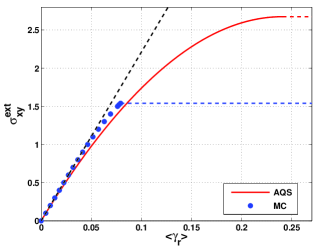
Figure 5: Stress-strain dependence under stress control for system I (see Fig. 2). The blue dots represent results of the Monte carlo simulations at $T=0.05$. The red line represents the prediction of the athermal quasistatic protocol (at $T=0$). Note that at zero temperature the yield stress is considerably larger.

Note that in Fig. 5 the Monte Carlo results are compared with an AQS stress controlled protocol (see in Subsect. III.1.2 how this is defined and computed). One is not surprised that at zero temperature the yield stress is considerably higher, and see below for more details. At this point it is enough to stress that $\sigma_{{}_{\rm Y}}$ depends on temperature if one can wait. Only at zero temperature this quantity is absolute in the sense that no waiting time is necessary for the system to fail. We return to this important issue in Sect. IV where we estimate the waiting time.

At finite temperature the internal stress, the energy and the strain fluctuate. The extent of these fluctuations at $T=0.05$ is shown in Fig. 6. Below the yield stress the system exhibits elastic behavior. When the yield stress is exceeded the system stays for a while in a series of metastable states (each of which exhibiting “elastic” behavior) whose life time becomes shorter and shorter until the simulation box collapses entirely. Note that these metastable states are the elastic branches that are seen very clearly in strain-controlled experiments, cf. Fig. 11 and Fig. 15. In that protocol the system loses energy and releases strain upon reaching a saddle point bifurcation and lands on the next elastic branch where it will stay forever if the strain does not increase. This is different from what is seen here, where once $\sigma_{{}_{\rm Y}}$ is exceeded the system fails, even though it may reside for a while on metastable states.

III.1.2 Zero temperature

In this subsection we show how to use the results of AQS strain control simulations to predict the physics of AQS stress control loading. Consider therefore the stress-strain relation using the athermal limit in the NVT ensemble defined by Eq. (18).

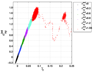
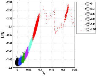
Figure 6: The dependence of the internal stress (top panel) and the energy (bottom panel) on the strain under stress-control for system I (see Fig. 2).

Imagine then that we run an AQS strain control simulation, and for every value of $\gamma$ we record the energy $U(\{{\bm{r}}_{i}\},\gamma)$ of the force free configuration after the non-affine relaxation took place. In order to find the minimum of the function (18) with regard to particle positions and the strain at a given external stress we have to study the dependence on strain of the generalized enthalpy. This dependence is shown in Fig. 7. We reiterate that the contribution $U(\{{\bm{r}}_{i}\},\gamma)$ is independent of stress and is defined by minimizing the energy at given strain via a relaxation of the particle positions.

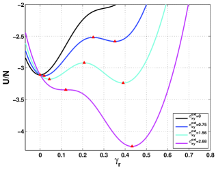
Figure 7: The strain dependence of the generalized enthalpy in the athermal case for system $\bf I$. The input from the strain controlled experiment is the first curve at $\sigma^{ext}_{xy}=0$. To this function we now add the term $-V\sigma^{ext}\gamma_{r}$ according to Eq. (18) to get all the other curves at varying values of $\sigma^{ext}_{xy}$.

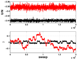
Figure 8: The evolution of the energy (top panel) and the strain $\gamma$ (botom panel) during the MC protocol for system II (see Fig. 2) for two values of the temperature. The external stress ${\bm{\sigma}}^{ext}_{xy}=0$, $T=0.05$ (black points) and $T=0.1$ (red points).

In the unstressed perfectly hexagonal structure there is only one minimum which is associated with a single reference state. Under applied stress there appears the metastable state separated from the global minimum by a barrier. The barrier height decreases with increasing stress and it disappears at the (zero-temperature) yield stress. We can now estimate the stress-strain relation from the series of curves that are shown in Fig. 7. As the stress increases the minimum of the curve shifts to higher values of strain. The stress vs strain dependence that is read in this way is shown in Fig. 5. We see the almost perfect correspondence between the two curves for small values of stress. The discrepancy at higher strains results from having different ensembles: in the AQS protocol the pressure varies non-monotonically with strain, in contrast to the Monte Carlo protocol at constant pressure, which in the present case is $P=0$.

The increase in pressure in this AQS stress-controlled procedure eliminates the failure of the material that we observe in the Monte Carlo stress-controlled protocol. Nevertheless we can predict the failure in the latter protocol from the former. We need to focus on that value of the stress where for the first time the depth of the two minima in Fig. 7 is the same. Note that this occurs at $\sigma=\sigma_{{}_{Y}}\approx 1.56$ in excellent agreement with the results shown in Fig. 5. Similar predictability will be shown below for the more complex examples.

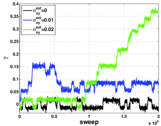
Figure 9: Evolution of the strain $\gamma$ in the MC simulations under applied external stress.

III.2 Hexagonal structure with defects

Our second system of interest is the hexagonal structure with a small number of defects whose concentration is about 2%, as seen in the lower panel of Fig. 2. Trajectories of measured values of the energy and the strain $\gamma$ as a function of the MC sweeps (here we used 2$\times 10^{6}$ sweeps) are shown in Fig. 8. In contrast to the perfect hexagonal structure the strain $\gamma$ displays at $T=0.05$ behavior typical to a bimodal distribution. Nevertheless, the comparison with results for higher temperature $T=0.1$ which exhibit the liquid behavior (see also IMPS07 ) shows that the system at lower temperature is in a solid state. A few examples of the same dependence under applied external stress are shown in Fig. 9. One can see that at relatively small values of external stress there are allowed transitions between available configurations. Then the applied stress exceeds some critical value ${\bf\sigma_{Y}}$ this dependence indicates the permanent deformation of the simulation cell via a number of metastable states (see Fig. 10).

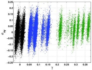
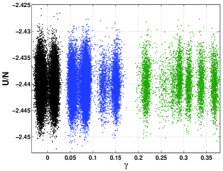
Figure 10: Dependence of the internal stress (top panel) and the energy (bottom panel) on the strain under stress-control for system II (see Fig. 2). Colors correspond to the legend in Fig. 9

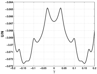
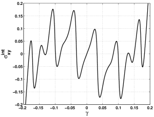
Figure 11: The simulation results in the frame of the AQS strain controlled protocol for the energy (top panel) and the internal stress (bottom panel).

The AQS strain controlled protocol (see Fig. (11)) now reveals that $U(\{{\bm{r}}_{i}\},\gamma)$ has a more complex landscape with a number of local minima. The athermal analysis of the generalized enthalpy can be done again as explained above. The applied external stress shifts equilibrium positions similarly to the MC results. Unfortunately, in the present case the amount of change in the pressure in the AQS protocol is too large to afford to say quantitative statement, leaving us with only a qualitative comparison.

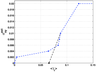
Figure 12: Stress-strain dependence under stress control for system II (see Fig. 2). In circles we show results of the Monte Carlo simulations with increasing value of $\sigma^{ext}_{xy}$. The black triangle represents the state obtained by an MC simulation at $\sigma^{ext}_{xy}=0$ starting from an initial condition which is a configuration found by the Monte Carlo protocol at $\sigma^{ext}_{xy}=0.01$.

Nevertheless, the simulation results show that transitions between different minima can soften the material enormously, leading to a yield stress that is enormously smaller than the corresponding one for the perfect hexagonal structure.

III.3 The glass

In the glass simulations we employed 400 particles in the simulation cell. A typical configuration of the binary mixture which produces our model glass is shown in Fig. 13. The reader can already guess that the increased disorder seen in this figure will translate to an increased complexity in the enthalpy landscape. Indeed, in Fig. 15 we show the enthalpy landscape as computed using the strain-controlled protocol and the changing landscapes upon the increase of the external stress.

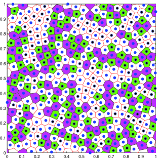
Figure 13: The structure of the binary mixture. Blue circles corresponds to A particles, black circles to particles B .

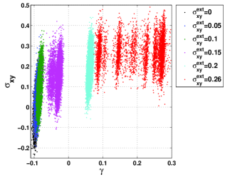
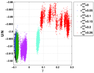
Figure 14: Dependence of the internal stress (top panel) and the energy (bottom panel) on strain under stress control for the glass model (see Fig. 13).

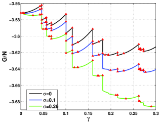
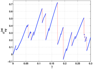
Figure 15: Top panel -the strain dependence of the generalized enthalpy in the athermal case for the glass. The input from the strain controlled experiment is the first curve at $\sigma^{ext}_{xy}=0$. To this function we now add the term $-V\sigma^{ext}\gamma$ according to Eq. (17) to get all the other curves at varying values of $\sigma^{ext}_{xy}$. Bottom panel-stress vs strain in a strain controlled simulation of the response of the binary glass at AQS conditions.

The corresponding results of the Monte Carlo simulation of the stress-strain dependence under stress control (in the glass simulations we use 2$\times 10^{6}$ sweeps) are shown in Fig. 16.

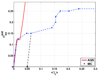
Figure 16: Stress-strain dependence of the binary glass. We again stress that in the stress control simulation the external stress is fixed and shown are the results for varying this fixed stress. In a triangle we show the state obtained by the MC simulation at $\sigma^{ext}_{xy}=0$ with initial configuration from the run at $\sigma^{ext}_{xy}=0.15$

To understand these results we again turn to the strain control experiment at $T=0$, for which we exhibit the stress vs strain trajectory in Fig. 15. Note again the immense difference between the two protocols: in strain controlled simulations one sees many plastic instabilities, and in each of them the system releases a part of the stress and a part of its mechanical energy. The strain is no longer a state variable due to the irreversible drops in energy. In contrast, in the stress control experiment one is bound to get stuck at one of the elastic branches as long as the stress is lower than the yield stress $\sigma_{{}_{\rm Y}}$, which in the present case is about 0.26.

At zero temperature the stress control experiment can exhibit only one instability where the system fails, when $\sigma^{ext}>\sigma_{{}_{\rm Y}}$. At finite temperatures one can observe multiple instabilities also in the stress control protocol as the system overcomes the barriers with the help of temperature fluctuations. Of course for a given external stress the waiting time will get longer and longer as the barrier increases, until the barrier that is associate with the zero-temperature $\sigma_{{}_{\rm Y}}$ is reached. Finally note also the precise correspondence between the zero-temperature and the finite temperature trajectories for small values of stress in Fig. 15. This correspondence can be maintained for much higher values of stress and strain by reducing the temperature.

An important point to discuss is the fact that the glass is much more cohesive than structure II even though is has many more “defects”. The reason for this lies in the microscopic interactions that are exhibited in Fig. 1. We see there that the AB interaction is considerably deeper than the AA interaction, meaning that the B particles act as pinning centers for the movement of A particles. This is in fact the deep reason why this mixture is a good glass former. For the structure II there is nothing that can pin the defects and they glide happily under any minute strain or stress, which explains the low yield stress of that structure compared to the glass. Indeed, this insight should be remembered whenever one wants to increase the cohesiveness of glasses, or to increase their shear modulus or their yield stress. One should add particles that act effectively as pinning centers, and see Ref. 14Gen for more details.

IV Temperature Effects and Waiting Times

At this point we focus on values of the stress that are close to the yields stress $\sigma_{{}_{\rm Y}}$, and particularly to the zero temperature value of this quantity (much of the discussion in this section is however relevant for any instability point at lower values of stress). Stressing the system at zero temperature will result in the system being stuck at a mean strain value $\langle\gamma\rangle$ that is less than the value of the strain which is associated with the position of the highest barrier, denoted conveniently as $\gamma_{{}_{\rm Y}}$. The question that we pose in this section is what is the waiting time $\tau$ (first passage time) for failure if the temperature is not zero. The problem is the classical one for escape over a barrier, but because this is a saddle node bifurcation there are some special characteristics that need to be taken into account.

The general expectation for the waiting time is that it should scale like

$$\tau\sim\omega^{-1}\exp{\Delta G/T}\ ,$$ (24)

where $\omega$ is the typical frequency of oscillations in the metastable minimum from which the system escapes, and as before $\Delta G$ is the enthalpic barrier that becomes a saddle together with the minimum at $\sigma=\sigma_{{}_{\rm Y}}$. One knows that in a saddle node bifurcation the frequency $\omega\sim\sqrt{\lambda}$ where $\lambda$ is the lowest eigenvalue of the Hessian matrix. The latter goes to zero at the saddle bifurcation like $\lambda\sim\sqrt{\gamma_{{}_{\rm Y}}-\gamma}$. As long as the harmonic approximation is relevant we can therefore write

$$\omega\sim(\gamma_{{}_{\rm Y}}-\gamma)^{1/4}\ .$$ (25)

On the other hand the height of the barrier scales like

$$\Delta G\sim\lambda^{3}\sim(\gamma_{{}_{\rm Y}}-\gamma)^{3/2}\ .$$ (26)

Using these scaling estimates in Eq. (24) we see that formally the waiting time diverges both at $(\gamma_{{}_{\rm Y}}-\gamma)\to 0$ and at $(\gamma_{{}_{\rm Y}}-\gamma)\to\infty$ with a minimum waiting time at a temperature dependent value $(\gamma_{{}_{\rm Y}}-\gamma)=(T/6)^{2/3}$. In reality however for any finite temperature we lose the relevance of the harmonic approximation in the limit $(\gamma_{{}_{\rm Y}}-\gamma)\to 0$, and we need to use the next, nonsingular, anharmonic correction to $\omega$. Also in the other limit, when $(\gamma_{{}_{\rm Y}}-\gamma)$ becomes large, we lose the relevance of the scaling law (26), destroying the singularity in this limit. Thus in both limits we predict a nonsingular waiting time. The conclusion is that a precise estimate of the waiting time calls for molecular dynamics simulations that are beyond the scope of this paper.

V Summary and Concluding Remarks

The main aim of this paper was to introduce a reliable simulational approach to stress controlled loading of systems at zero or finite temperatures. The method of variable shape appears stable and useful, and we exemplified it for a perfect hexagonal structure, the same structure with a few defects, and a generic binary glass in 2-dimensions. The main conclusion is that the type of mechanical instabilities encountered in stress-controlled protocols is one and the same as those seen in strain-controlled protocols, i.e saddle node bifurcations in which the Hessian matrix becomes unstable, sending one of its eigenvalues to zero. As a result, the knowledge of the possible instabilities that are found in AQS strain-controlled simulations is very helpful forr understanding what is happening in stress-controlled simulations, even at finite temperature. Of course, the difference in the type of ensemble is not unimportant, and deviations in the system response from one protocol to the other are expected and also found. Nevertheless approximating the enthalpy landscape with the help of the AQS stain controlled simulations is shown to be very useful in clarifying what one should expect in a finite temperature stress-controlled protocol. Examples of this understanding were given for all the three examples treated in this paper. Finally we examined the issue of the waiting time for yield in stress-controlled simulations, making full use of the identification of the instabilities as saddle-node bifurcations. The conclusion there was that one can see a decrease or increase in the waiting time as a function of the distance from the instability, but that eventually the waiting time is not singular.

We reiterate that all our stress-controlled simulations here were performed for zero pressure. It would be interesting in the future to follow up on the present study with stress-controlled simulations when different component of the stress tensor are kept constant, to see how the response of the system depends on such details. We hope to report on such simulations in forthcoming publications. In addition, and maybe even more importantly, the present protocol allows a very precise study of the yielding process itself. This study will be reported elsewhere.

- (1) Mechanics of Solids. Ed. C. Truesdell (Encyclopedia of Physics. Chief Editor S. Flugge, Vol. YIa/1): J. F. Bell, The Experimental Foundations of Solid Mechanics. Berlin-Heidelberg-New York, Springer-Verlag, 813 p. (1973)
- (2) A. H. Cottrell, Dislocations and plastic flow in crystals. University Press, Oxford (1953).
- (3) C. Maloney, A. Lemaître, Universal breakdown of elasticity at the onset of material failure. Phys. Rev. Lett. 93, 195501 (2004).
- (4) S. Karmakar, A. Lemaître, E. Lerner, I. Procaccia, Predicting plastic flow events in athermal shear-strained amorphous solids. Phys. Rev. Lett. 104, 215502 (2010).
- (5) D. L. Malandro and D. J. Lacks, Molecular-Level Mechanical Instabilities and Enhanced Self-Diffusion in Flowing Liquids, Phys. Rev. Lett. 81, 5576 (1998).
- (6) M. L. Falk, J. S. Langer, Dynamics of viscoplastic deformation in amorphous solids. Phys. Rev. E 57, 7192-7205 (1998).
- (7) D. Rodney, C. A. Schuh, Yield stress in metallic glasses: The jamming-unjamming transition studied through Monte Carlo simulations based on the activation-relaxation technique. Phys. Rev. B 80, 184203 (2009).
- (8) M. Parrinello, A. Rahman, Crystal structure and pair potential: A molecular-dynamics study. Phys. Rev. Lett. 45, 1196-199 (1980).
- (9) M. Parrinello, A. Rahman, Polymorphic transitions in single crystals: A new molecular dynamics method. J. Appl. Phys. 52, 7182-7190 (1981).
- (10) K. W. Wojciechovski, K. V. Tretiakov, M. Kowalik, Elastic properties of dence solid phases of hard cyclic pentamers and heptamers in two dimensions. Phys. Rev. E 67, 036121 (2003).
- (11) J. R. Ray, A. Rahman, Statistical ensembles and molecular dynamics studies of anisotropic solids. J. Chem. Phys. 80, 4423-4428 (1984).
- (12) J. V. Lill, J. Q. Broughhton, Atomistic simulations incorporating nonlinear elasticity: Slow-stress relaxation and symmetry breaking. Phys. Rev. B 49, 11619-11633 (1994).
- (13) A. Lemaître, C. Maloney, Sum rules for the quasi-statc and visco-elastic respones of disordered solids at zero temperature. J. Stat. Phys. 123, 415-453 (2006).
- (14) J. Wang, J. Li, S. Yip, Mechanical instabilities of homogneous crystals. Phys. Rev. B 52, 12627-12635 (1995).
- (15) J.J. Gilman, in M.D. Furnish, N.N. Thadhani and Y. Horie, eds. Shock Compression of Condensed Matter, page 36, (AIP 2002).
- (16) W. Kob, H. C. Andersen, Scaling behavior in the -relaxation regime of a supercooled Lennard-Jones mixture. Phys. Rev. Lett. 73 1376-1379 (1994).
- (17) R. Brüning, D. A. St-Onge1, S. Patterson, W. Kob, Glass transitions in one-, two-, three-, and four-dimensional binary Lennard-Jones systems. J. Phys.: Condens. Matter 21, 035117 (2009).
- (18) E. Aharonov , E. Bouchbinder , H. G. E. Hentschel , V. Ilyin , N. Makedonska , I. Procaccia and N. Schupper, Direct identification of the glass transition: Growing length scale and the onset of plasticity. Euro.Phys. Lett.77, 56002 (2007).
- (19) V. Ilyin, N. Makedonska, I. Procaccia, N. Scupper, Mechanical properties of glass forming systems. Phys. Rev. E 76, 052401 (2007).
- (20) O. Gendelman, J. Ashwin, P. Mishra, I. Procaccia and K. Samwer, Acta Materialia,63, 209,(2014).