Learning Word Representations
with Hierarchical Sparse Coding
Abstract
We propose a new method for learning word representations using hierarchical regularization in sparse coding inspired by the linguistic study of word meanings. We show an efficient learning algorithm based on stochastic proximal methods that is significantly faster than previous approaches, making it possible to perform hierarchical sparse coding on a corpus of billions of word tokens. Experiments on various benchmark tasks—word similarity ranking, analogies, sentence completion, and sentiment analysis—demonstrate that the method outperforms or is competitive with state-of-the-art methods. Our word representations are available at http://www.ark.cs.cmu.edu/dyogatam/wordvecs/.
1 Introduction
When applying machine learning to text, the classic categorical representation of words as indices of a vocabulary fails to capture syntactic and semantic similarities that are easily discoverable in data (e.g., pretty, beautiful, and lovely have similar meanings, opposite to unattractive, ugly, and repulsive). In contrast, recent approaches to word representation learning apply neural networks to obtain dense, low-dimensional, continuous embeddings of words (Bengio et al., 2003; Mnih and Teh, 2012; Collobert et al., 2011; Huang et al., 2012; Mikolov et al., 2010, 2013b; Lebret and Collobert, 2014).
In this work, we propose an alternative approach based on decomposition of a high-dimensional matrix capturing surface statistics of association between a word and its “contexts” with sparse coding. As in past work, contexts are words that occur nearby in running text (Turney and Pantel, 2010). Learning is performed by minimizing a reconstruction loss function to find the best factorization of the input matrix.
The key novelty in our method is to govern the relationships among dimensions of the learned word vectors, introducing a hierarchical organization imposed through a structured penalty known as the group lasso (Yuan and Lin, 2006). The idea of regulating the order in which variables enter a model was first proposed by Zhao et al. (2009), and it has since been shown useful for other applications (Jenatton et al., 2011). Our approach is motivated by coarse-to-fine organization of words’ meanings often found in the field of lexical semantics (see §2.2 for a detailed description), which mirrors evidence for distributed nature of hierarchical concepts in the brain (Raposo et al., 2012). Related ideas have also been explored in syntax (Petrov and Klein, 2008). It also has a foundation in cognitive science, where hierarchical structures have been proposed as representations of semantic cognition (Collins and Quillian, 1969). We show a stochastic proximal algorithm for hierarchical sparse coding that is suitable for problems where the input matrix is very large and sparse. Our algorithm enables application of hierarchical sparse coding to learn word representations from a corpus of billions of word tokens and 400,000 word types.
On standard evaluation tasks—word similarity ranking, analogies, sentence completion, and sentiment analysis—we find that our method outperforms or is competitive with the best published representations.
2 Model
2.1 Background and Notation
The observable representation of word is taken to be a vector of cooccurrence statistics with different contexts. Most commonly, each context is a possible neighboring word within a fixed window.111Others include: global context (Huang et al., 2012), multilingual context (Faruqui and Dyer, 2014), geographic context (Bamman et al., 2014), brain activation data (Fyshe et al., 2014), and second-order context (Schutze, 1998). Following many others, we let be the pointwise mutual information (PMI) between the occurrence of context word within a five-word window of an occurrence of word (Turney and Pantel, 2010; Murphy et al., 2012; Faruqui and Dyer, 2014).
In sparse coding, the goal is to represent each input vector as a sparse linear combination of basis vectors. Given a stacked input matrix , where is the number of words, we seek to minimize:
| (1) |
where is the dictionary of basis vectors, is the set of matrices whose columns have small (e.g., less than or equal to one) norm, is the code matrix, is a regularization hyperparameter, and is the regularizer. Here, we use the squared loss for the reconstruction error, but other loss functions could also be used (Lee et al., 2009). Note that it is not necessary, although typical, for to be less than (when , it is often called an overcomplete representation). The most common regularizer is the penalty, which results in sparse codes. While structured regularizers are associated with sparsity as well (e.g., the group lasso encourages group sparsity), our motivation is to use to encourage a coarse-to-fine organization of latent dimensions of the learned representations of words.
2.2 Structured Regularization for Word Representations
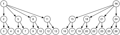
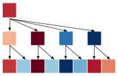
For , we design a forest-structured regularizer that encourages the model to use some dimensions in the code space before using other dimensions. Consider the trees in Figure 1. In this example, there are 13 variables in each tree, and 26 variables in total (i.e., ), each corresponding to a latent dimension for one particular word. These trees describe the order in which variables “enter the model” (i.e., take nonzero values). In general, a node may take a nonzero value only if its ancestors also do. For example, nodes 3 and 4 may only be nonzero if nodes 1 and 2 are also nonzero. Our regularizer for column of , denoted by (in this example, ), for the trees in Figure 1 is:
where returns the (possibly empty) set of descendants of node . Jenatton et al. (2011) proposed a related penalty with only one tree for learning image and document representations.
Let us analyze why organizing the code space this way is helpful in learning better word representations. Recall that the goal is to have a good dictionary and code matrix . We apply the structured penalty to each column of . When we use the same structured penalty in these columns, we encode an additional shared constraint that the dimensions of that correspond to top level nodes should focus on “general” contexts that are present in most words. In our case, this corresponds to contexts with extreme PMI values for most words, since they are the ones that incur the largest losses. As we go down the trees, more word-specific contexts can then be captured. As a result, we have better organization across words when learning their representations, which also translates to a more structured dictionary . Contrast this with the case when we use unstructured regularizers that penalize each dimension of independently (e.g., lasso). In this case, each dimension of has more flexibility to pay attention to any contexts (the only constraint that we encode is that the cardinality of the model should be small). We hypothesize that this is less appropriate for learning word representations, since the model has excessive freedom when learning on noisy PMI values, which translates to poor .
The intuitive motivation for our regularizer comes from the field of lexical semantics, which often seeks to capture the relationships between words’ meanings in hierarchically-organized lexicons. The best-known example is WordNet (Miller, 1995). Words with the same (or close) meanings are grouped together (e.g., professor and prof are synonyms), and fine-grained meaning groups (“synsets”) are nested under coarse-grained ones (e.g., professor is a hyponym of academic). Our hierarchical sparse coding approach is still several steps away from inducing such a lexicon, but it seeks to employ the dimensions of a distributed word representation scheme in a similar coarse-to-fine way. In cognitive science, such hierarchical organization of semantic representations was first proposed by Collins and Quillian (1969).
2.3 Learning
Learning is accomplished by minimizing the function in Eq. 1, with the group lasso regularization function described in §2.2. The function is not convex with respect to and , but it is convex with respect to each when the other is fixed. Alternating minimization routines have been shown to work reasonably well in practice for such problems (Lee et al., 2007), but they are too expensive here due to:
-
•
The size of ( and are each on the order of ).
-
•
The many overlapping groups in the structured regularizer .
One possible solution is based on the online dictionary learning method of Mairal et al. (2010). For iterations, we:
-
•
Sample a mini-batch of words and (in parallel) solve for each one’s using the alternating directions method of multipliers, shown to work well for overlapping group lasso problems (Qin and Goldfarb, 2012; Yogatama and Smith, 2014).222Since our groups form tree structures, other methods such as FISTA (Jenatton et al., 2011) could also be used.
-
•
Update using the block coordinate descent algorithm of Mairal et al. (2010).
Finally, we parallelize solving for all columns of , which are separable once is fixed. In our experiments, we use this algorithm for a medium-sized corpus.
The main difficulty of learning word representations with hierarchical sparse coding is that the size of the input matrix can be very large. When we use neighboring words as the contexts, the numbers of rows and columns are the size of the vocabulary. For a medium-sized corpus with hundreds of millions of word tokens, we typically have one or two hundred thousand unique words, so the above algorithm is still applicable. For a large corpus with billions of word tokens, this number can easily double or triple, making learning very expensive. We propose an alternative learning algorithm for such cases.
We rewrite Eq. 1 as:
where (abusing notation) denotes the -th row vector of and denotes the -th column vector of (recall that ). Instead of considering all elements of the input matrix, our algorithm approximates the solution by using only non-zero entries in the input matrix . At each iteration, we sample a non-zero entry and perform gradient updates to the corresponding row and column .
We directly penalize columns of by their squared norm as an alternative to constraining columns of to have unit norm. The advantage of this transformation is that we have eliminated a projection step for columns of . Instead, we can include the gradient of the penalty term in the stochastic gradient update. We apply the proximal operator associated with as a composition of elementary proximal operators with no group overlaps, similar to Jenatton et al. (2011). This can be done by recursively visiting each node of a tree and applying the proximal operator for the group lasso penalty associated with that node (i.e., the group lasso penalty where the node is the topmost node and the group consists of the node and all of its descendants). The proximal operator associated with node , denoted by , is simply the block-thresholding operator for node and all its descendants.
Since each non-zero entry only depends on and , we can sample multiple non-zero entries and perform the updates in parallel as long as they do not share and . In our case, where and are on the order of hundreds of thousands and we only have tens or hundreds of processors, finding non-zero elements that do not violate this constraint is easy. There are typically a huge number of non-zero entries (on the order of billions). Using a sampling procedure that favors entries with higher (absolute) PMI values can lead to reasonably good word representations faster. We sample a non-zero entry with probability proportional to its absolute value. This also justifies using only the non-zero entries, since the probability of sampling zero entries is always zero.333In practice, we can use a faster approximation of this sampling procedure by uniformly sampling a non-zero entry and multiplying its gradient by a scaling constant proportional to its absolute PMI value. We summarize our learning algorithm in Algorithm 1.
3 Experiments
We present a controlled comparison of the forest regularizer against several strong baseline word representations learned on a fixed dataset, across several tasks. In §3.4 we compare to publicly available word vectors trained on different data.
3.1 Setup and Baselines
We use the WMT-2011 English news corpus as our training data.444http://www.statmt.org/wmt11/ The corpus contains about 15 million sentences and 370 million words. The size of our vocabulary is 180,834.555 We replace words with frequency less than 10 with #rare# and numbers with #number#.
In our experiments, we use forests similar to those in Figure 1 to organize the latent word space. Note that the example has 26 nodes (2 trees). We choose to evaluate performance with (4 trees) and (40 trees).666In preliminary experiments we explored binary tree structures and found they did not work as well; we leave a more extensive exploration of tree structures to future work. We denote the sparse coding method with regular penalty by SC, and our method with structured regularization (§2.2) by forest. We set . In this first set of experiments with a medium-sized corpus, we use the online learning algorithm of Mairal et al. (2010).
We compare with the following baseline methods:
- •
-
•
Mikolov et al. (2010): a recursive neural network (RNN) language model. We obtain an implementation from http://rnnlm.org/.
- •
-
•
Mikolov et al. (2013b): a log bilinear model that predicts a word given its context (continuous bag of words, CBOW), trained using negative sampling (Mikolov et al., 2013a). We obtain an implementation from https://code.google.com/p/word2vec/.
-
•
Mikolov et al. (2013b): a log bilinear model that predicts context words given a target word (skip gram, SG), trained using negative sampling (Mikolov et al., 2013a). We obtain an implementation from https://code.google.com/p/word2vec/.
Our focus here is on comparisons of model architectures. For a fair comparison, we train all competing methods on the same corpus using a context window of five words (left and right). For the baseline methods, we use default settings in the provided implementations (or papers, when implementations are not available and we reimplement the methods). We also trained the last two baseline methods with hierarchical softmax using a binary Huffman tree instead of negative sampling; consistent with Mikolov et al. (2013a), we found that negative sampling performs better and relegate hierarchical softmax results to supplementary materials.
3.2 Evaluation
We evaluate on the following benchmark tasks.
Word similarity
The first task evaluates how well the representations capture word similarity. For example beautiful and lovely should be closer in distance than beautiful and unattractive. We evaluate on a suite of word similarity datasets, subsets of which have been considered in past work: WordSim 353 (Finkelstein et al., 2002), rare words (Luong et al., 2013), and many others; see supplementary materials for details. Following standard practice, for each competing model, we compute cosine distances between word pairs in word similarity datasets, then rank and report Spearman’s rank correlation coefficient (Spearman, 1904) between the model’s rankings and human rankings.
Syntactic and semantic analogies
The second evaluation dataset is two analogy tasks proposed by Mikolov et al. (2013b). These questions evaluate syntactic and semantic relations between words. There are 10,675 syntactic questions (e.g., walking : walked :: swimming : swam) and 8,869 semantic questions (e.g., Athens : Greece :: Oslo :: Norway). In each question, one word is missing, and the task is to correctly predict the missing word. We use the vector offset method (Mikolov et al., 2013b) that computes the vector . We only consider a question to be answered correctly if the returned vector () has the highest cosine similarity to the correct answer (in this example, ).
Sentence completion
The third evaluation task is the Microsoft Research sentence completion challenge (Zweig and Burges, 2011). In this task, the goal it to choose from a set of five candidate words which one best completes a sentence. For example: Was she his {client, musings, discomfiture, choice, opportunity}, his friend, or his mistress? (client is the correct answer). We choose the candidate with the highest average similarity to every other word in the sentence.777We note that unlike matrix decomposition based approaches, some of the neural network based models can directly compute the scores of context words given a possible answer (Mikolov et al., 2013b). We choose to use average similarities for a fair comparison of the representations.
Sentiment analysis
The last evaluation task is sentence-level sentiment analysis. We use the movie reviews dataset from Socher et al. (2013). The dataset consists of 6,920 sentences for training, 872 sentences for development, and 1,821 sentences for testing. We train -regularized logistic regression to predict binary sentiment, tuning the regularization strength on development data. We represent each example (sentence) as an -dimensional vector constructed by taking the average of word representations of words appearing in that sentence.
The analogy, sentence completion, and sentiment analysis tasks are evaluated on prediction accuracy.
3.3 Results
Table 1 shows results on all evaluation tasks for and . Runtime will be discussed in §3.5. In the similarity ranking and sentiment analysis tasks, our method performed the best in both low and high dimensional embeddings. In the sentence completion challenge, our method performed best in the high-dimensional case and second-best in the low-dimensional case. Importantly, forest outperforms PCA and unstructured sparse coding (SC) on every task. We take this collection of results as support for the idea that coarse-to-fine organization of latent dimensions of word representations captures the relationships between words’ meanings better compare to unstructured organization.
| Task | PCA | RNN | NCE | CBOW | SG | SC | forest | |
|---|---|---|---|---|---|---|---|---|
| 52 | Word similarity | 0.39 | 0.26 | 0.48 | 0.43 | 0.49 | 0.49 | 0.52 |
| Syntactic analogies | 18.88 | 10.77 | 24.83 | 23.80 | 26.69 | 11.84 | 24.38 | |
| Semantic analogies | 8.39 | 2.84 | 25.29 | 8.45 | 19.49 | 4.50 | 9.86 | |
| Sentence completion | 27.69 | 21.31 | 30.18 | 25.60 | 26.89 | 25.10 | 28.88 | |
| Sentiment analysis | 74.46 | 64.85 | 70.84 | 68.48 | 71.99 | 75.51 | 75.83 | |
| 520 | Word similarity | 0.50 | 0.31 | 0.59 | 0.53 | 0.58 | 0.58 | 0.66 |
| Syntactic analogies | 40.67 | 22.39 | 33.49 | 52.20 | 54.64 | 22.02 | 48.00 | |
| Semantic analogies | 28.82 | 5.37 | 62.76 | 12.58 | 39.15 | 15.46 | 41.33 | |
| Sentence completion | 30.58 | 23.11 | 33.07 | 26.69 | 26.00 | 28.59 | 35.86 | |
| Sentiment analysis | 81.70 | 72.97 | 78.60 | 77.38 | 79.46 | 78.20 | 81.90 |
| Task | CBOW | SG | forest |
|---|---|---|---|
| Syntactic | 61.37 | 63.61 | 65.11 |
| Semantic | 23.13 | 54.41 | 52.07 |
| Models | W. Sim. | Syntactic | Semantic | Sentence | Sentiment | ||
|---|---|---|---|---|---|---|---|
| CW | 50 | 130,000 | (6,225) 0.51 | (10,427) 12.34 | (8,656) 9.33 | (976) 24.59 | 69.36 |
| RNN-DC | 100,232 | (6,137) 0.32 | (10,349) 10.94 | (7,853) 2.60 | (964) 19.81 | 67.76 | |
| HLBL | 246,122 | (6,178) 0.11 | (10,477) 8.98 | (8,446) 1.74 | (990) 19.90 | 62.33 | |
| NNSE | 34,107 | (3,878) 0.23 | (5,114) 1.47 | (1,461) 2.46 | (833) 0.04 | 64.80 | |
| HPCA | 178,080 | (6,405) 0.29 | (10,553) 10.42 | (8,869) 3.36 | (993) 20.14 | 67.49 | |
| forest | 52 | 180,834 | (6,525) 0.52 | (10,675) 24.38 | (8,733) 9.86 | (1,004) 28.88 | 75.83 |
Analogies
Unlike others tasks, our results on the syntactic and semantic analogies tasks are below state-of-the-art performance from previous work (for all models). We hypothesize that this is because performing well on these tasks requires training on a bigger corpus. We combine our WMT-2011 corpus with other news corpora and Wikipedia to obtain a corpus of 6.8 billion words. The size of the vocabulary of this corpus is 401,150. We retrain three models that are scalable to a corpus of this size: CBOW, SG, and forest;888Our NCE implementation is not optimized and therefore not scalable. with to balance the trade-off between training time and performance ( does not perform as well, and is computationally expensive). For forest, we use the fast learning algorithm in §2.3, since the online learning algorithm of Mairal et al. (2010) does not scale to a problem of this size. We report accuracies on the syntactic and semantic analogies tasks in Table 2. All models benefit significantly from a bigger corpus, and the performance levels are now comparable with previous work. On the syntactic analogies task, forest is the best model. On the semantic analogies task, SG outperformed forest, and they both are better than CBOW.
3.4 Other Comparisons
In Table 3, we compare with five other baseline methods for which we do not train on our training data but pre-trained 50-dimensional word representations are available:
-
•
Collobert et al. (2011): a neural network language model trained on Wikipedia data for 2 months (CW).999http://ronan.collobert.com/senna/
-
•
Huang et al. (2012): a neural network model that uses additional global document context (RNN-DC).101010http://goo.gl/Wujc5G
-
•
Mnih and Hinton (2008): a log bilinear model that predicts a word given its context, trained using hierarchical softmax (HLBL).111111http://metaoptimize.com/projects/wordreprs/ (Turian et al., 2010)
-
•
Murphy et al. (2012): a word representation trained using non-negative sparse embedding (NNSE) on dependency relations and document cooccurrence counts.121212Obtained from http://www.cs.cmu.edu/~bmurphy/NNSE/. These vectors were learned using sparse coding, but using different contexts (dependency and document cooccurrences), a different training method, and with a nonnegativity constraint. Importantly, there is no hierarchy in the code space, as in forest.131313We found that NNSE trained using our contexts performed very poorly; see supplementary materials.
-
•
Lebret and Collobert (2014): a word representation trained using Hellinger PCA (HPCA).141414http://lebret.ch/words/
These methods were all trained on different corpora, so they have different vocabularies that do not always include all of the words found in the tasks. We estimate performance on the items for which prediction is possible, and show the count for each method in Table 3. This comparison should be interpreted cautiously since many experimental variables are conflated; nonetheless, forest performs strongly.
3.5 Discussion
Our method produces sparse word representations with exact zeros. We observe that the sparse coding method without a structured regularizer produces sparser representations, but it performs worse on our evaluation tasks, indicating that it zeroes out meaningful dimensions. For forest with and , the average numbers of nonzero entries are 91% and 85% respectively. While our word representations are not extremely sparse, this makes intuitive sense since we try to represent about 180,000 contexts in only 52 (520) dimensions. We also did not tune . As we increase , we get sparser representations.
In terms of running time, forest is reasonably fast to learn. We use the online dictionary learning method for and on a medium-sized corpus. For , the dictionary learning step took about 30 minutes (64 cores) and the overall learning procedure took approximately 2 hours (640 cores). For , the dictionary learning step took about 1.5 hours (64 cores) and the overall learning procedure took approximately 20 hours (640 cores). For comparison, the SG model took about 1.5 hours and 5 hours for and using a highly optimized implementation from the author’s website (with no parallelization). On a large corpus with 6.8 billion words and vocabulary size of about 400,000, forest with Algorithm 1 took about 2 hours (16 cores) while SG took about 6.5 hours (16 cores) for .
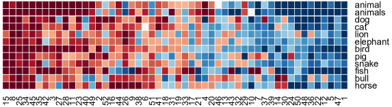
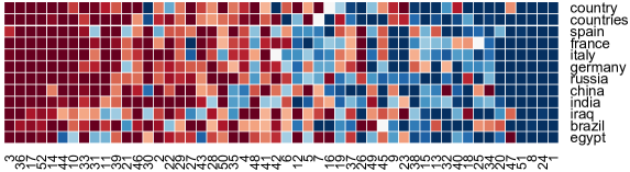
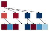
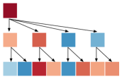
We visualize our word representations (forest) related to animals (10 words) and countries (10 words). We show the coefficient patterns for these words in Figure 2. We can see that in both cases, there are dimensions where the coefficient signs (positive or negative) agree for all 10 words (they are mostly on the right and left sides of the plots). Note that the dimensions where all the coefficients agree are not the same in animals and countries. The larger magnitude of the vectors for more abstract concepts (animal, animals, country, countries) is suggestive of neural imaging studies that have found evidence of more global activation patterns for processing superordinate terms (Raposo et al., 2012). In Figure 3, we show tree visualizations of coefficients of word representations for animal, horse, and elephant. We show one tree for (there are four trees in total, but other trees exhibit similar patterns). Coefficients that differ in sign mostly correspond to leaf nodes, validating our motivation that top level nodes should focus more on “general” contexts (for which they should be roughly similar for animal, horse, and elephant) and leaf nodes focus on word-specific contexts. One of the leaf nodes for animal is driven to zero, suggesting that more abstract concepts require fewer dimensions to explain.
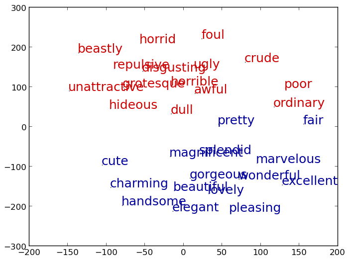
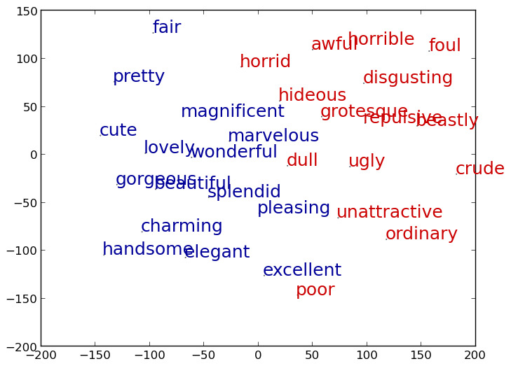
For forest and SG with , we project the learned word representations into two dimensions using the t-SNE tool (van der Maaten and Hinton, 2008) from http://homepage.tudelft.nl/19j49/t-SNE.html. We show projections of words related to the concept “good” vs. “bad” in Figure 4.151515Since t-SNE is a non-convex method, we run it 10 times and choose the plots with the lowest t-SNE error. See supplementary materials for “man” vs. “woman,” as well as 2-dimensional projections of NCE.
4 Conclusion
We introduced a new method for learning word representations based on hierarchical sparse coding. The regularizer encourages hierarchical organization of the latent dimensions of vector-space word embeddings. We showed that our method outperforms state-of-the-art methods on word similarity ranking, syntactic analogy, sentence completion, and sentiment analysis tasks.
Acknowledgements
The authors thank anonymous reviewers, Sam Thomson, Bryan R. Routledge, Jesse Dodge, and Fei Liu for helpful feedback on an earlier draft of this paper. This work was supported by the National Science Foundation through grant IIS-1352440, the Defense Advanced Research Projects Agency through grant FA87501420244, and computing resources provided by Google and the Pittsburgh Supercomputing Center.
References
- Bamman et al. (2014) Bamman, D., Dyer, C., and Smith, N. A. (2014). Distributed representations of situated language. In Proc. of ACL.
- Bengio et al. (2003) Bengio, Y., Ducharme, R., Vincent, P., and Jauvin, C. (2003). A neural probabilistic language model. Journal of Machine Learning Research, 3, 1137–1155.
- Collins and Quillian (1969) Collins, A. M. and Quillian, M. R. (1969). Retrieval time from semantic memory. Journal of Verbal Learning and Verbal Behaviour, 8, 240–247.
- Collobert et al. (2011) Collobert, R., Weston, J., Bottou, L., Karlen, M., Kavukcuoglu, K., and Kuska, P. (2011). Natural language processing (almost) from scratch. Journal of Machine Learning Research, 12, 2461–2505.
- Faruqui and Dyer (2014) Faruqui, M. and Dyer, C. (2014). Improving vector space word representations using multilingual correlation. In Proc. of EACL.
- Finkelstein et al. (2002) Finkelstein, L., Gabrilovich, E., Matias, Y., Rivlin, E., Solan, Z., Wolfman, G., and Ruppin, E. (2002). Placing search in context: The concept revisited. ACM Transactions on Information Systems, 20(1), 116–131.
- Fyshe et al. (2014) Fyshe, A., Talukdar, P. P., Murphy, B., and Mitchell, T. M. (2014). Interpretable semantic vectors from a joint model of brain- and text- based meaning. In Proc. of ACL.
- Gutmann and Hyvarinen (2010) Gutmann, M. and Hyvarinen, A. (2010). Noise-contrastive estimation: A new estimation principle for unnormalized statistical models. In Proc. of AISTATS.
- Huang et al. (2012) Huang, E. H., Socher, R., Manning, C. D., and Ng, A. Y. (2012). Improving word representations via global context and multiple word prototypes. In Proc. of ACL.
- Jenatton et al. (2011) Jenatton, R., Mairal, J., Obozinski, G., and Bach, F. (2011). Proximal methods for hierarchical sparse coding. Journal of Machine Learning Research, 12, 2297–2334.
- Lebret and Collobert (2014) Lebret, R. and Collobert, R. (2014). Word embeddings through hellinger PCA. In Proc. of EACL.
- Lee et al. (2007) Lee, H., Battle, A., Raina, R., and Ng, A. Y. (2007). Efficient sparse coding algorithms. In Proc. of NIPS.
- Lee et al. (2009) Lee, H., Raina, R., Teichman, A., and Ng, A. Y. (2009). Exponential family sparse coding with application to self-taught learning. In Proc. of IJCAI.
- Luong et al. (2013) Luong, M.-T., Socher, R., and Manning, C. D. (2013). Better word representations with recursive neural networks for morphology. In Proc. of CONLL.
- Mairal et al. (2010) Mairal, J., Bach, F., Ponce, J., and Sapiro, G. (2010). Online learning for matrix factorization and sparse coding. Journal of Machine Learning Research, 11, 19–60.
- Mikolov et al. (2010) Mikolov, T., Martin, K., Burget, L., Cernocky, J., and Khudanpur, S. (2010). Recurrent neural network based language model. In Proc. of Interspeech.
- Mikolov et al. (2013a) Mikolov, T., Sutskever, I., Chen, K., Corrado, G., and Dean, J. (2013a). Distributed representations of words and phrases and their compositionality. In Proc. of NIPS.
- Mikolov et al. (2013b) Mikolov, T., Chen, K., Corrado, G., and Dean, J. (2013b). Efficient estimation of word representations in vector space. In Proc. of ICLR Workshop.
- Miller (1995) Miller, G. A. (1995). Wordnet: A lexical database for english. Communications of the ACM, 38(11), 39–41.
- Mnih and Hinton (2008) Mnih, A. and Hinton, G. (2008). A scalable hierarchical distributed language model. In Proc. of NIPS.
- Mnih and Teh (2012) Mnih, A. and Teh, Y. W. (2012). A fast and simple algorithm for training neural probabilistic language models. In Proc. of ICML.
- Murphy et al. (2012) Murphy, B., Talukdar, P., and Mitchell, T. (2012). Learning effective and interpretable semantic models using non-negative sparse embedding. In Proc. of COLING.
- Petrov and Klein (2008) Petrov, S. and Klein, D. (2008). Sparse multi-scale grammars for discriminative latent variable parsing. In Proc. of EMNLP.
- Qin and Goldfarb (2012) Qin, Z. T. and Goldfarb, D. (2012). Structured sparsity via alternating direction methods. Journal of Machine Learning Research, 13, 1435–1468.
- Raposo et al. (2012) Raposo, A., Mendes, M., and Marques, J. F. (2012). The hierarchical organization of semantic memory: Executive function in the processing of superordinate concepts. NeuroImage, 59, 1870–1878.
- Schutze (1998) Schutze, H. (1998). Automatic word sense discrimination. Computational Linguistics - Special issue on word sense disambiguation, 24(1), 97–123.
- Socher et al. (2013) Socher, R., Perelygin, A., Wu, J., Chuang, J., Manning, C., Ng, A., and Potts, C. (2013). Recursive deep models for semantic compositionality over a sentiment treebank. In Proc. of EMNLP.
- Spearman (1904) Spearman, C. (1904). The proof and measurement of association between two things. The American Journal of Psychology, 15, 72–101.
- Turian et al. (2010) Turian, J., Ratinov, L., and Bengio, Y. (2010). Word representations: A simple and general method for semi-supervised learning. In Proc. of ACL.
- Turney and Pantel (2010) Turney, P. D. and Pantel, P. (2010). From frequency to meaning: Vector space models of semantics. Journal of Artificial Intelligence Research, 37, 141–188.
- van der Maaten and Hinton (2008) van der Maaten, L. and Hinton, G. (2008). Visualizing data using t-sne. Journal of Machine Learning Research, 9, 2579–2605.
- Yogatama and Smith (2014) Yogatama, D. and Smith, N. A. (2014). Making the most of bag of words: Sentence regularization with alternating direction method of multipliers. In Proc. of ICML.
- Yuan and Lin (2006) Yuan, M. and Lin, Y. (2006). Model selection and estimation in regression with grouped variables. Journal of the Royal Statistical Society, Series B, 68(1), 49–67.
- Zhao et al. (2009) Zhao, P., Rocha, G., and Yu, B. (2009). The composite and absolute penalties for grouped and hierarchical variable selection. The Annals of Statistics, 37(6A), 3468–3497.
- Zweig and Burges (2011) Zweig, G. and Burges, C. J. C. (2011). The microsoft research sentence completion challenge. Technical report, Microsoft Research Technical Report MSR-TR-2011-129.