Electron correlation in solids via density embedding theory

Abstract

Density matrix embedding theory (Phys. Rev. Lett. 109, 186404 (2012)) and density embedding theory (Phys. Rev. B 89, 035140 (2014)) have recently been introduced for model lattice Hamiltonians and molecular systems. In the present work, the formalism is extended to the ab initio description of infinite systems. An appropriate definition of the impurity Hamiltonian for such systems is presented and demonstrated in cases of 1, 2 and 3 dimensions, using coupled cluster theory as the impurity solver. Additionally, we discuss the challenges related to disentanglement of fragment and bath states. The current approach yields results comparable to coupled cluster calculations of infinite systems even when using a single unit cell as the fragment. The theory is formulated in the basis of Wannier functions but it does not require separate localization of unoccupied bands. The embedding scheme presented here is a promising way of employing highly accurate electronic structure methods for extended systems at a fraction of their original computational cost.

I Introduction

Electron correlation plays a crucial role in understanding most physical phenomena in molecules and extended systems. While highly accurate many-body approaches can be nowadays routinely employed in molecular systems, solid state applications remains dominated by density functional theory (DFT). Despite the undeniable success of DFT in extended systems, Parr and Yang (1994); Becke (2014); Burke (2012) there are significant limitations appearing from the approximate form of the exchange-correlation functional Mattsson (2002) and much work remains to be done in order to ensure systematically improvable predictions. Cohen et al. (2008); Perdew et al. (2008); Marques et al. (2011); Koller et al. (2013); Bulik et al. (2013); Heyd and Scuseria (2004); Heyd et al. (2005); Lucero et al. (2011, 2012); El-Mellouhi et al. (2013) An alternative route for incorporating electron correlations is to employ wavefunction-based methods. Recently, significant progress in applying such many-body theories for solid state problems has been made. Hirata (2008); Hirata and Shimazaki (2009); Shiozaki and Hirata (2010); Booth et al. (2013); Voloshina and Paulus (2014)

Size-extensive, wavefunction-based approaches to solids treat the system as a whole, imposing translational symmetry and Brillouin zone integration. Finite order perturbation theory Ye et al. (1993); Suhai (1994, 1995); Sun and Bartlett (1996, 1997); Hirata and Iwata (1998); Ayala et al. (2001); Marsman et al. (2009); Grüneis et al. (2010) and coupled cluster (CC) methods Förner et al. (1997); Reinhardt (2000); Hirata et al. (2004); Sun and Bartlett (1999) have been formulated and implemented for infinite systems. Alternatively, the numerical complexity associated with numerous electronic degrees of freedom in solids has been simplified, for example, by means of the method of increments. Stoll (1992a, b, c); Yu et al. (1997); Paulus (2006)

In the present work, electron correlation in extended systems is accounted for via an embedding approach. The infinite periodic problem is transformed into one of a small fragment (unit cell) entangled with an effective bath. In order to define the bath, we employ the recently introduced density embedding theory (DET), Bulik et al. (2014) which is a simplification of density matrix embedding theory (DMET). Knizia and Chan (2012, 2013) Here, an approximate solution to the infinite periodic system, typically Hartree-Fock, is used to construct two basis sets. The first basis is associated with a small part of the lattice (fragment) whereas the second is used to describe the excluded complement (bath). Subsequently, one solves the many-body problem for the fragment plus bath, a so-called impurity problem. In this way, correlations between the fragment and the rest of the system are represented by a many-electron environment, not a single-particle potential. Knizia and Chan (2013) The Hartree-Fock (HF) choice for an approximate solution of the infinite solid affords the desired bases in a trivial algebraic manner via diagonalization. Moreover, the resulting Hamiltonian describing the fragment-bath interaction is defined in a much smaller single-particle Hilbert space as compared to the full lattice Hamiltonian. Thus, this construction opens the possibility of employing highly accurate many-body techniques to tackle extended systems.

Indeed, DMET and DET with exact diagonalizationKnizia and Chan (2012, 2013); Booth, G. H. and Chan, G. K-L. (2013); Bulik et al. (2014) and density matrix renormalization groupChen et al. (2014) as impurity solvers have been shown to provide high-quality descriptions of model Hamiltonians and molecular systems. In the present work we extend the applicability of this novel approximation to realistic extended systems. Such problems seem a promising niche for this embedding scheme. The definition of fragment is naturally dictated by the periodicity of the system which greatly simplifies the procedure. We propose a way of defining the local Hamiltonian that guarantees exactness of mean-field in mean-field embedding and facilitates coping with the Coulomb problem in solids. Additionally, we discuss practical issues related to preparing the fragment and bath basis for an infinite number of electrons and the problem of disentangled states.

While in the current work we benchmark the DET scheme by describing the fragment-bath interaction at the coupled cluster level of theory, we stress that the methodology is flexible enough to accommodate any correlated wavefunction method. Indeed, the purpose of DET is to provide a finite, small dimension effective Hamiltonian which should account for locally important degrees of freedom. Then, any many-body technique may be employed to solve the impurity problem at hand. In particular, very accurate and computationally affordable schemes Jiménez-Hoyos et al. (2013); Rodríguez-Guzmán et al. (2013) may be used to study extended systems with realistic unit cell sizes.

II Theory and formalism

In order to keep this paper self-contained, we present in this section a basic introduction to density matrix and density embedding theories. More details can be found in the original papers. Knizia and Chan (2012, 2013); Booth, G. H. and Chan, G. K-L. (2013); Bulik et al. (2014); Chen et al. (2014) Subsequently, we discuss the changes required to apply the formalism to the ab initio Hamiltonian of extended systems. This includes the Schmidt decomposition of Slater determinants for infinite systems and the formulation of an impurity Hamiltonian that allows us to deal with the Coulomb divergence in solids. Unless otherwise specified, single-particle indices denote both spin and spatial coordinates. In the context of periodic systems, cell coordinates are implicitly included except when confusion may arise.

II.1 Mean-field based embedding theories

Density matrix embedding theory and its simplification, density embedding theory, are projections of the exact Hamiltonian onto a basis obtained by Schmidt decomposition of the ground state wavefunction $|\Psi\rangle$. To be precise, one may cast $|\Psi\rangle$ into Knizia and Chan (2012)

$$|\Psi\rangle=\sum_{i}\lambda_{i}|\alpha_{i}\rangle|\beta_{i}\rangle,$$ (1)

where $|\alpha\rangle$ represents the part of the system of interest, the fragment, whereas $|\beta\rangle$ represents the rest of the system, the bath. With such states at hand, an impurity Hamiltonian is defined,

$$\hat{H}_{\textrm{imp}}=\sum_{ijkl}|\alpha_{i}\rangle|\beta_{j}\rangle\langle\alpha_{i}|\langle\beta_{j}|\hat{H}|\alpha_{k}\rangle|\beta_{l}\rangle\langle\alpha_{k}|\langle\beta_{l}|.$$ (2)

which has the same ground state as the exact Hamiltonian.Knizia and Chan (2012) The fragment and bath basis states are, in principle, many-electron states.

In order to make calculations practical, DMET and DET replace the exact ground state with a mean-field approximation, i.e. $|\Psi\rangle$ is replaced with $|\Phi\rangle=\Pi_{p}a{}^{\dagger}_{p}|0\rangle$, where $a{}^{\dagger}_{p}$ creates a hole state $|\phi_{p}\rangle$ and $|0\rangle$ is the bare vacuum. The hole creation operators are obtained from a mean-field approximation, here the Hartree-Fock transformation $\mathbb{D}$ of bare fermion operators $c^{\dagger}$:

$$a{}^{\dagger}_{p}=\sum_{\mu}\mathbb{D}_{\mu p}c{}^{\dagger}_{\mu}.$$ (3)

The mean-field solution is obtained for the Hamiltonian of interest augmented with an effective one-body potential $v$,

$$\hat{H}=\sum_{\mu\nu}h_{\mu\nu}c{}^{\dagger}_{\mu}c_{\nu}+\frac{1}{4}\sum_{\mu\nu\lambda\sigma}V_{\mu\nu\lambda\sigma}c{}^{\dagger}_{\mu}c{}^{\dagger}_{\nu}c_{\sigma}c_{\lambda}+\sum_{\mu\nu}v_{\mu\nu}c{}^{\dagger}_{\mu}c_{\nu}.$$ (4)

The meaning of this potential will soon become apparent.

With the above approximation, the task of performing the Schmidt decomposition of the wavefunction describing the whole system amounts to a rather trivial algebraic problem Klich (2006). Defining single particle basis associated with a chosen subsystem of the entire problem, $|F\rangle$, one constructs a projection operator onto the fragment $\hat{P}_{F}=\sum_{i}|F_{i}\rangle\langle F_{i}|$ and its complement $\hat{P}_{B}=\hat{\mathbb{I}}-\hat{P}_{F}$. The latter projects onto the bath states. With such tools at hand, one may construct an overlap matrix $\mathbb{M}$,

$$\mathbb{M}_{pq}=\langle\phi_{q}|\hat{P}_{F}|\phi_{p}\rangle,$$ (5)

where indices $p$ and $q$ denote the hole states. Diagonalizing the above overlap matrix $\mathbb{V}d\mathbb{V}^{\dagger}=\mathbb{M}$ yields at most min($n_{e}$,$n_{F}$) eigenvalues $d_{i}$ different from zero where $n_{e}$ and $n_{F}$ denote the number of electrons in the system and the number of single-particle states associated with the fragment, respectively. The eigenvectors corresponding to such eigenvalues are then normalized to construct fragment ($|f\rangle$) and bath ($|b\rangle$) states

$$|f_{i}\rangle =\sum_{p}\frac{\mathbb{V}{}^{\star}_{pi}}{\sqrt{d_{i}}}\hat{P}_{F}|\phi_{p}\rangle$$

$$|b_{i}\rangle =\sum_{p}\frac{\mathbb{V}{}^{\star}_{pi}}{\sqrt{1-d_{i}}}\hat{P}_{B}|\phi_{p}\rangle.$$ (6)

The states that correspond to zero eigenvalue are called cores and are discarded from consideration in the impurity problem.

In practical applications, one would like to retain all the fragment states. This requires special care when the eigenvalues $d$ are close to 1 or 0. Such complications are addressed in Appendix A.2. Right now, let us stress the consequences of the above approximation which is a key step in the present work. The most prominent result is that the Schmidt decomposition yields single-particle bases that can be further employed in the construction of the impurity Hamiltonian. This fact greatly facilitates computations. Additionally, the number of entangled states (or equivalently the number of non-zero eigenvalues $d$) is defined by the fragment single-particle basis. If one chooses the fragment to be small, accurate many-body techniques can be applied to solve the impurity problem, which we now proceed to introduce.

Let us define creation operators in the impurity basis: $f^{\dagger}$, $b^{\dagger}$ and $e^{\dagger}$; $f^{\dagger}$ and $b^{\dagger}$ are associated with fragment and bath states, respectively. We will use $e^{\dagger}$ for general states which can be either fragment or bath. The impurity problem is defined by the Hamiltonian,

$$\hat{H}_{\textrm{imp}} =\sum_{ee^{\prime}}\tilde{h}_{ee^{\prime}}e{}^{\dagger}e^{\prime}+\frac{1}{4}\sum_{ee^{\prime}e^{\prime\prime}e^{\prime\prime\prime}}\tilde{V}_{ee^{\prime}e^{\prime\prime}e^{\prime\prime\prime}}e{}^{\dagger}e{}^{\prime\dagger}e^{\prime\prime\prime}e^{\prime\prime}$$

$$+\sum_{bb^{\prime}}\tilde{v}_{bb^{\prime}}b{}^{\dagger}b^{\prime},$$ (7)

where $\tilde{h}$ and $\tilde{V}$ are one- and (antisymmetrized) two-body terms of the Hamiltonian projected onto the embedding basis. The additional potential $\tilde{v}$, acting only in the bath subspace of the impurity, is introduced to enforce a suitable chosen convergence criterion. In the present work, we make a diagonal ansatz for the effective potential ($\tilde{v}_{ij}=v\delta_{ij}$ hence $v_{\mu\nu}=v\delta_{\mu\nu}$ in Eq. 4), which corresponds to a chemical potential in the bath. We find such a potential by requiring the proper number of electrons in the fragment, on average. Let us stress that, for periodic systems, the average number of electrons per unit cell is known and well defined. The reader is referred to Ref. Bulik et al., 2014 for other possible choices of the effective potential.

At this point, let us make a few remarks concerning the meaning of the impurity Hamiltonian. Assuming that $\mathbb{M}$ contains $n_{F}$ eigenvalues different from 1 or 0, this Hamiltonian describes a system of $n_{F}$ particles in $2n_{F}$ spin orbitals. Solving the Hamiltonian in the Hilbert space of the impurity corresponds to a Fock space calculation in the fragment subspace. The bath can be considered as a reservoir of electrons or holes.

Having solved the impurity Hamiltonian, the energy density (energy per fragment) is subsequently computed as

$$E=\sum_{fe}\tilde{h}_{fe}\gamma_{ef}+\frac{1}{4}\sum_{fee^{\prime}e^{\prime\prime}}\tilde{V}_{fee^{\prime}e^{\prime\prime}}\Gamma_{e^{\prime}e^{\prime\prime}fe},$$ (8)

with $\gamma_{ee^{\prime}}=\langle e^{\prime\dagger}e\rangle$ and $\Gamma_{ee^{\prime}e^{\prime\prime}e^{\prime\prime\prime}}=\langle e^{\dagger}e^{\prime\dagger}e^{\prime\prime\prime}e^{\prime\prime}\rangle$ being one- and two-particle density matrices of the impurity wavefunction. Again, index $f$($e$) denotes fragment (fragment and bath) single-particle states.

We note that the DET energy is not an expectation value of the true Hamiltonian with an N-particle wavefunction. It is therefore not an upper bound of the true ground state energy.

II.2 Schmidt decomposition for periodic systems

Density embedding calculations on a truly infinite system require a suitable single-particle basis associated with a fragment. In the present work, we employ the maximally localized Wannier functions Marzari et al. (2012); Löwdin (1950); Pipek and Mezey (1989); Zicovich-Wilson et al. (2001) obtained by localization of canonical mean-field crystalline orbitals. In other words, we form a unitary transformation of mean-field basis $|\psi_{n\vec{k}}\rangle$, where $\vec{k}$ labels irreducible representation of the translational group Pisani (1996); Kudin and Scuseria (1998) and $n$ is a band index. This yields an orthonormal set $|F_{i\vec{G}}\rangle$, where $i$ labels a basis in given cell $\vec{G}$. The orthonormality condition reads, Marzari et al. (2012)

$$\langle F_{i\vec{G}}|F_{j\vec{G}^{\prime}}\rangle=\delta_{ij}\delta_{\vec{G}\vec{G}^{\prime}}.$$ (9)

A few comments are called for at this point. Firstly, during the localization process, we must allow for mixing of hole and particle states. Therefore, there is no need for localizing the particle (unoccupied) orbitals by themselves. In our numerical approach, we did not encounter serious difficulties converging the Wannier basis required by the present formalism. Secondly, as we explain in more details in Appendix A.1, one may desire to truncate the space treated in the impurity Hamiltonian only to levels around the Fermi energy. This is accomplished simply by choosing a subset of energy bands for the localization. In other words, only a limited set of the highest valence bands and the lowest conduction bands may be employed while forming $|F_{i\vec{G}}\rangle$ bases. As the number of bands used during the localization process is equal to the number of fragment states per unit cell, a suitable truncation criterion may be used to further limit the single-particle Hilbert space of the impurity Hamiltonian without sacrificing relevant physics.

Analogously, one needs to perform the localization of the hole states, yielding $|\phi_{p\vec{G}}\rangle$, which constitutes the $p^{\textrm{th}}$ hole state associated with cell $\vec{G}$. Whenever a truncation of the conduction band occurs while forming the fragment states, the same truncation should be done during the formation of the hole states.

Now, one is in a position to compute the overlap matrix of Eq. 5,

$$\mathbb{M}{}_{pq}^{\vec{G}\vec{G}^{\prime}}=\langle\phi_{q\vec{G}^{\prime}}|\hat{P}_{F}|\phi_{p\vec{G}}\rangle=\sum_{i}\langle\phi_{q\vec{G}^{\prime}}|F_{i\vec{0}}\rangle\langle F_{i\vec{0}}|\phi_{p\vec{G}}\rangle,$$ (10)

needed to define the fragment and bath states of the impurity basis. In the above formula, the summation over the fragment states is limited to the reference cell $\vec{0}$. If embedding of more than one cell is needed, the summation over the entire embedded cluster must be performed. With the aid of the above matrix, fragment and bath states are formed according to Eq. II.1 keeping in mind that index $p$ in those equations includes a cell coordinate.

At this point we would like to note that the localization of the hole states and the local nature of the fragment single-particle basis allows for effective truncation of the formally infinite summation over the entire crystal. Indeed, one may limit the summation over cells when $\langle F_{i\vec{0}}|\phi_{p\vec{G}}\rangle\to 0$ as $|\vec{G}|$ increases. The localization of the hole states therefore dictates a natural length scale one has to consider during DET calculations.

II.3 Definition of the impurity Hamiltonian

Having established a formalism for constructing the embedding basis, let us turn our attention to the definition of the impurity Hamiltonian. A Hamiltonian for a realistic crystalline material can be written as

$$\hat{H}=E_{NN}+\hat{V}_{Ne}+\hat{V}_{ee}+\hat{T}=H_{0}+\hat{h}+\hat{V},$$ (11)

where $E_{NN}$ is the nuclear repulsion energy, $\hat{V}_{Ne}$ and $\hat{V}_{ee}$ are the electrostatic electron-nucleus and electron-electron interactions, respectively; $\hat{T}$ is the kinetic energy operator. Those terms can be then arranged into constant ($H_{0}$) and one- and two-body Hamiltonians ($\hat{h}$ and $\hat{V}$, respectively). As described in the literature, Kudin and Scuseria (2000); Pisani (1996); Jaffe and Hess (1996); Dovesi et al. (1983) the summation of an infinite number of electrostatic terms has to be handled with care in order to avoid divergences and loss of accuracy. Analogous problems may arise while projecting the Hamiltonian onto the embedding basis. In order to deal with such complications, we propose to first recast the Hamiltonian into second-quantized form with the aid of the mean-field Fock matrix

$$F_{\mu\nu}=h_{\mu\nu}+\sum_{\lambda\sigma}V_{\mu\lambda\nu\sigma}\gamma_{\sigma\lambda},$$ (12)

as

$$\hat{H} =E_{0}-\sum_{\mu\nu}F{}_{\mu\nu}\gamma_{\nu\mu}+\frac{1}{2}\sum_{\mu\nu\lambda\sigma}V_{\mu\lambda\nu\sigma}\gamma_{\sigma\lambda}\gamma_{\nu\mu}$$

$$+\sum_{\mu\nu}\Big{(}F_{\mu\nu}-V_{\mu\lambda\nu\sigma}\gamma_{\sigma\lambda}\Big{)}c{}^{\dagger}_{\nu}c_{\nu}+\frac{1}{4}\sum_{\mu\nu\lambda\sigma}V_{\mu\nu\lambda\sigma}c{}^{\dagger}_{\mu}c{}^{\dagger}_{\nu}c_{\sigma}c_{\lambda}$$ (13)

In the expression above, $E_{0}=EN$ where $E$ is the mean-field energy per unit cell and $N$ is the number of cells. Again, the individual terms in the summation are not necessarily convergent. For example, the constant $\frac{1}{2}\sum_{\mu\nu\lambda\sigma}V_{\mu\lambda\nu\sigma}\gamma_{\sigma\lambda}\gamma_{\nu\mu}$ describing the electron-electron interaction energy is divergent and has no meaningful thermodynamic limit, if evaluated separately. Similarly, $\sum_{\lambda\sigma}V_{\mu\lambda\nu\sigma}\gamma_{\sigma\lambda}$, which contributes to the one-body Hamiltonian above, gives rise to divergent matrix elements. For these reasons, we propose to express all quantities in the embedding basis, before the summation is performed. In other words, we separately project the mean-field potential, the density matrix and the two-body interaction onto the embedding basis, i.e. $F_{\mu\nu}\to\tilde{F}_{ee^{\prime}}$, $\gamma_{\mu\nu}\to\tilde{\gamma}_{ee^{\prime}}$ and $V_{\mu\nu\lambda\sigma}\to\tilde{V}_{ee^{\prime}e^{\prime\prime}e^{\prime\prime\prime}}$. While the two-body interaction is projected without any modifications, let us explicitly write the one-body part of the impurity Hamiltonian, $\tilde{h}$, and the constant term, $\tilde{E_{0}}$,

$$\tilde{h}_{ee^{\prime}} =\tilde{F}_{ee^{\prime}}-\sum_{e^{\prime\prime}e^{\prime\prime\prime}}\tilde{V}_{ee^{\prime\prime}e^{\prime}e^{\prime\prime\prime}}\tilde{\gamma}_{e^{\prime\prime\prime}e^{\prime\prime}}$$ (14)

$$\tilde{E_{0}} =EN_{F}-\sum_{fe}\Big{(}\tilde{F}_{fe}-\frac{1}{2}\sum_{e^{\prime}e^{\prime\prime}}\tilde{V}_{fe^{\prime}ee^{\prime\prime}}\tilde{\gamma}_{e^{\prime\prime}e^{\prime}}\Big{)}\tilde{\gamma}_{ef},$$ (15)

where again, $E$ denotes the mean-field energy per unit cell, whereas $N_{F}$ is the number of unit cells in the fragment. As the reader may readily notice, the summation restriction to the fragment basis only has been imposed on the constant term above. The reason for such truncation shall become clear soon.

The construction above constitutes an approximate way of projecting the Hamiltonian. Let us therefore discuss the physical motivation behind it. As shown in Ref. Bulik et al., 2014 and expanded upon in the Appendix below, the mean-field one-particle density matrix and mean-field Fock matrix commute with each other after projection onto the embedding basis, i.e., $[\tilde{\gamma},\tilde{F}]=0$. Moreover, $\tilde{\gamma}$ is idempotent. Inserting $\tilde{\gamma}$ as an initial guess for the impurity Hamiltonian as define above yields a Fock matrix that is equal to the Fock matrix of the whole system projected onto the embedding basis,

$$F{}^{\textrm{imp}}_{ee^{\prime}}=\tilde{h}_{ee^{\prime}}+\sum_{e^{\prime\prime}e^{\prime\prime\prime}}\tilde{V}_{ee^{\prime\prime}e^{\prime}e^{\prime\prime\prime}}\tilde{\gamma}_{e^{\prime\prime\prime}e^{\prime\prime}}=\tilde{F}_{ee^{\prime}}.$$ (16)

The mean-field solution of the impurity problem is therefore the crystal density matrix in the embedding basis. Furthermore, computing the energy according to Eq. 8 (with a constant term defined by Eq. 15) reveals that the mean-field energy of the fragment is just the energy per unit cell multiplied by the number of cells taken as fragment constituents. In the above, we have set the effective potential, present in Eq. 4 to zero. We conclude that the current definition of the impurity problem ensures exactness of mean-field in mean-field embedding. Furthermore, the solution corresponds to a vanishing effective potential $v$. We would like to stress that the exactness of the mean-field in mean-field embedding has been numerically demonstrated for DMET in Ref. Knizia and Chan, 2013.

Finally, let us note that for nontrivial calculations, that is when a correlated theory is used as an impurity solver, the effective potential has to be optimized and included in the impurity Hamiltonian as well as the full crystal Hamiltonian. In the present work, the diagonal ansatz for the effective potential allows us to eliminate these terms from the mean-field Fock matrix of the crystal as it cannot change the mean-field solution. Therefore, the construction of the embedding basis and the impurity Hamiltonian is performed only once during the calculation. The value of the effective potential is determined in the embedding basis only.

III Computational details

The construction of Wannier functions has been implemented in the Gaussian Developement Version Frisch et al. that has also been used to perform the periodic Hartree-Fock calculations. The crystalline orbital localization has been performed by adapting the scheme the of Ref. Zicovich-Wilson et al., 2001, where the Boys localization is replaced by the Pipek-Mezey localization Pipek and Mezey (1989) with the Löwdin population. Löwdin (1950) For 1D systems, we have used a $\vec{k}$-point mesh of at least 400 points; for 2D and 3D, 4000 and 70000 $\vec{k}$-points have been used, respectively. The hermitized density matrices for coupled cluster with double (CCD) and single and double (CCSD) excitations were obtained using the linear response formalism. Gauss and Stanton (1995); Scheiner et al. (1987)

The most diffuse basis functions of the 6-31G basis Hehre et al. (1972); Dill and Pople (1975) were changed to 0.35, 0.30, and 0.20 for the carbon, nitrogen and boron atoms, respectively.

In all calculations, eigenvalue thresholds of the Schmidt decomposition for retaining the bath states was set to 10^-6. The fragment states corresponding to eigenvalues that were closer to 0 or 1 than this threshold were constructed according to the formalism outlined in Appendix A.2.

The number of cells used in the Schmidt decomposition has been decided by a commutation criterion between mean-field Fock and density matrices after projection onto the embedding basis, $\sum_{ee^{\prime}}|(\tilde{F}\tilde{\gamma})_{ee^{\prime}}-(\tilde{\gamma}\tilde{F})_{ee^{\prime}}|$. The values of this norm are reported for the calculations in the subsequent section.

IV Results and discussion

IV.1 1D carbon systems

In this section, we asses the performance of DET on three carbon polymers, polyyne (C$\equiv$C)_∞, polyacetylene (CH$=$CH)_∞, and polyethylene (CH₂$-$CH₂)_∞. In the present work, we adopt the geometries from Ref. Hirata et al., 2004. The geometrical parameters are $r_{\mathrm{C}\equiv\mathrm{C}}=1.263\AA$, $r_{\mathrm{C}-\mathrm{C}}=1.132\AA$ for polyyne, $r_{\mathrm{C}=\mathrm{C}}=1.369\AA$, $r_{\mathrm{C}-\mathrm{C}}=1.426\AA$, $r_{\mathrm{C}-\mathrm{H}}=1.091\AA$, $\angle_{\mathrm{C}=\mathrm{C}-\mathrm{C}}=124.5^{\circ}$, $\angle_{\mathrm{C}=\mathrm{C}-\mathrm{H}}=118.3^{\circ}$ for polyacetylene, and $r_{\mathrm{C}-\mathrm{C}}=1.534\AA$, $r_{\mathrm{C}-\mathrm{H}}=1.100\AA$, $\angle_{\mathrm{C}-\mathrm{C}-\mathrm{C}}=113.7^{\circ}$, $\angle_{\mathrm{H}-\mathrm{C}-\mathrm{H}}=106.1^{\circ}$ for polyethylene. In order to gain better insight into the performance of the DET approximation, we have additionally deformed the above systems by keeping all variables, apart from the carbon-carbon bonds, fixed, while scaling the carbon-carbon bonds uniformly with a parameter $\alpha$. In all calculations, the $1s$ orbitals of carbon were eliminated from consideration in DET and coupled cluster calculations. DET($n$) denotes calculations with $n$ unit cells used as a fragment.

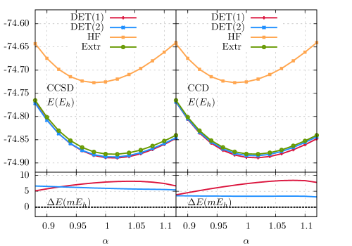
Figure 1: Energy per unit cell profile for polyyne (C$\equiv$C)_∞ with respect to uniform deformation (see text for details) with STO-3G basis. The results of DET(1) and DET(2) with CCSD (left panel) and CCD (right panel) as impurity solver calculations are compared to CCSD (left panel) and CCD (right panel) oligomeric extrapolation (Extr) and Hartree-Fock (HF). For clarity the difference between DET and extrapolated data is displayed in the bottom panel.

Figure 2: Same as Fig.1 with 6-31G basis.

Let us begin the discussion with the most challenging system for the embedding calculation, polyyne. In this case, one expects that the correlation energy contribution to the unit cell would have the slowest decay. Hirata et al. (2004) The results are shown in Fig. 1 and Fig. 2. The extrapolated CCD and CCSD results were obtained according to

$$E_{\textrm{Extr}}(n)=E_{HF}+E_{\textrm{corr}}(n)-E_{\textrm{corr}}(n-1)$$ (17)

where $E_{HF}$ is HF energy per unit cell of infinite system and $E_{\textrm{corr}}(n)$ is the correlation energy of the $n$-unit oligomer with a hydrogen atom as the terminal group. For the case of STO-3G basis, extrapolations for $n=8$ and $n=7$ differ by no more than 0.1 $mE_{h}$; in the case of the 6-31G basis, we have used $n=9$ which differs from $n=8$ by at most 0.2 $mE_{h}$. We deem these results sufficiently converged for the purpose of the presented figures. Our extrapolated CCSD correlation energy value for the STO-3G basis and $\alpha=1$, of -155.45 $mE_{h}$ agrees well with -155.53 $mE_{h}$ reported in Ref. Hirata et al., 2004. In the DET calculations, the number of cells used for the Schmidt decomposition guaranteed that the norm of the commutator of full-system Fock and density matrices projected onto the embedding basis to be at most $3\times 10^{-6}$.

As is clear from Fig. 1, the DET calculations with a single unit cell chosen as a fragment agree well with the extrapolated thermodynamic limit values both for CCSD and CCD as the impurity solver. The maximum discrepancy is below 10 $mE_{h}$; this translates to an energy difference on the level of $5\%$. Investigating the shape of the energy profile as a function of the uniform stretching parameter $\alpha$, we find the overall agreement satisfactory. The inclusion of electron correlation clearly favors a more stretched configuration. Apparently, DET calculations appropriately capture this trend. One may also notice that including two unit cells as the fragment yields results that are closer to the extrapolated CCSD and CCD results.

Increasing the size of the basis set to 6-31G does not lead to a deterioration of the DET results. As is clear from Fig. 2, the single-cell DET calculations are again in good agreement with the extrapolated values. The absolute difference does increase slightly but so does the correlation energy. The overall shape of the energy profile is well reproduced by DET. The bonds elongation caused by correlation is well captured.

Let us comment on the size of the impurity problem for polyyne. In the case of the STO-3G basis, there are 8 fragment and 8 bath orbitals for the single cell case, with the impurity bearing 16 electrons. This illustrates how effective the present embedding scheme is in truncating the size of the single-particle Hilbert space of the problem.

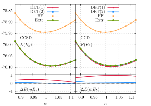
Figure 3: Same as Fig.1 for polyacetylene.

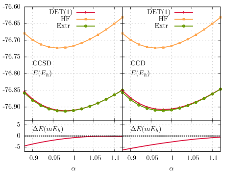
Figure 4: Same as Fig.1 for polyacetylene with the 6-31G basis.

The next polymeric system under investigation is polyacetylene. For this example, the extrapolated CCSD and CCD correlation energy from 8 and 7 cells differed by less than 0.1 $mE_{h}$ for both STO-3G and 6-31G bases. The value of $E_{\textrm{corr}}$ for CCSD with $\alpha=1$, -146.4 $mE_{h}$, coincides with the one reported in Ref. Hirata et al., 2004. The number of cells used in the Schmidt decomposition guaranteed that the norm of the commutator between the mean-field density and Fock matrices in the embedding basis is below $10^{-6}$.

Analogously to polyyne, one notices in Fig. 3 and Fig. 4 that correlation favors a more elongated carbon-carbon bond. Both DET and extrapolated oligomeric results agree quantitatively. For the STO-3G basis, even the DET(1) calculation yields results within 4 $mE_{h}$ from extrapolated values, a result that is greatly improved by enlarging the embedded fragment to two cells. Regardless, the DET approximation with both CCD and CCSD as impurity solvers yield results that are rather parallel to the thermodynamic limit ones. With the increased size of the basis set, the agreement remains satisfactory. Though the curvature of the energy profile obtined with DET(1) deviates slightly from the extrapolated data, especially for contracted systems ($\alpha\leq 0.95$), the difference is not large. Again, one has to keep in mind that DET calculations are done employing a significantly truncated single-particle basis. For the STO-3G basis, the impurity problem with single cell models the infinite system with a Hamiltionian that describes merely 20 electrons in 20 orbitals (10 fragment and 10 bath states).

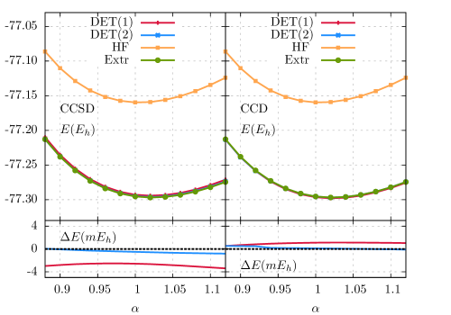
Figure 5: Same as Fig.1 for polyethylene.

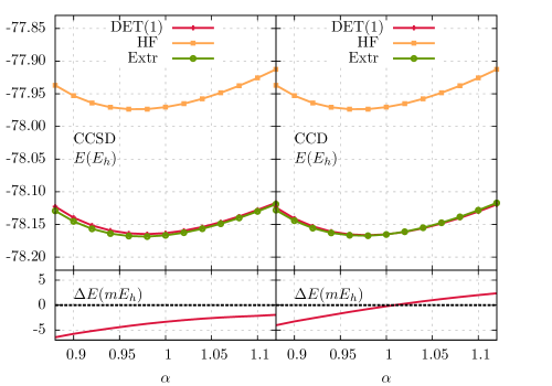
Figure 6: Same as Fig.1 for polyethylene with the 6-31G basis.

The last 1D polymer studied is polyethylene. Just as in the case of polyacetylene, the difference between the extrapolated CCD and CCSD energy using 8 and 7 cells was well below 0.1 $mE_{h}$. For STO-3G and $\alpha=1$, our extrapolated CCSD correlation energy per unit cell, -135.7 $mE_{h}$, coincides with the value reported by Hirata. Hirata et al. (2004) The number of cells included in the Schmidt decomposition guaranteed that the norm of the commutator between the mean-field Fock and density matrices is below $10^{-6}$ after projection onto embedding basis.

For polyethylene, the STO-3G DET(1) results (Fig. 5) coincide very well with the extrapolated oligomeric data. The small difference is almost constant over the studied values of the $\alpha$ stretching parameter. Increasing the embedded fragment to two cells brings the discrepancy almost to zero. With the bigger basis, 6-31G, once again we observe very good overall agreement between DET and extrapolated data. The maximum difference occurs for the more contracted geometry. Just as in all previous systems, one observes stabilization of a more elongated structure due to correlation effects. Again, let us stress that, within the DET approximation, modeling the infinite system with an impurity problem of 24 electrons in 24 orbitals (12 fragment states and 12 bath states), for the example of DET(1) STO-3G calculations, allows one to obtain a high degree of agreement with the full periodic CCD and CCSD calculations. One should however keep in mind, that the physical interpretation of the impurity problem differs from the true Hamiltonian. In the former, the CC(S)D method is used to effectively perform a Fock space calculation in the unit cell with the aid of an entangled bath. On the other hand, for the full Hamiltonian one considers excitations of the electrons of the entire periodic system.

IV.2 2D and 3D: boron nitride and diamond

Figure 7: Energy per unit cell as a function of lattice parameter of honeycomb boron nitride lattice. The DET(1) calculations with CCSD and CCD as impurity solvers are compared with HF for STO-3G (left) and 6-31G (right).

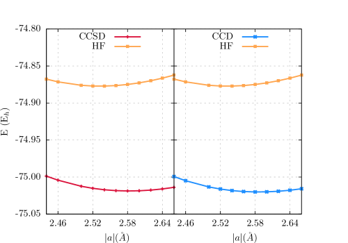
Figure 8: Energy per unit cell as a function of lattice parameter (primitive unit cell) for diamond. The DET(1) calculations with CCSD (left) and CCD (right) as impurity solvers are compared with HF for the STO-3G basis.

In this section, we proceed to investigate prototypical 2D and 3D systems. The 2D structure was obtained assuming infinitely separated boron nitride sheets of hexagonal BN Liu et al. (2014); Oshima and Nagashima (1997) yielding a graphene-like honeycomb lattice. We performed a single unit embedding with CCSD and CCD as an impurity solver. The number of cells included in the Schmidt decomposition was chosen to provide the norm of the commutator of the mean-field and Fock matrices in the embedding basis below 10^-6. The two lowest bands were excluded from consideration, which corresponds to freezing 1$s$ orbitals of boron and nitrogen in the CC calculations.

In Fig 7, we present the dependence of the energy per unit cell with respect to the translation vector defining the underlying honeycomb lattice. As the reader may readily notice, our DET calculations predict noticeable impact from the inclusion of the single excitation in the CC impurity solver. For both, the STO-3G and 6-31G bases, the CCSD energy is consistently below the CCD energy by about 10-20 $mE_{h}$. Nonetheless, the shape of the curves around the equilibrium point are rather similar. The impact of the electron correlation clearly shifts the position of the optimal structure towards longer translation vectors as compared to mean-field calculations. We also note that the lattice constant obtained with single cell DET embedding is larger than that reported one for the hexagonal BN. Liu et al. (2014); Andreev and Lundström (1994) While this elongation is due to the inclusion of only a single sheet, lack of solid substrate or the deficiency of the employed basis set is beyond the scope of the present work. However, we would like to stress the key point of current work. Namely, the size of the Hilbert space of impurity Hamiltonian is small and independent of the dimensionality of the problem. The calculations for the single cell with STO-3G basis required explicit correlated treatment of 16 electrons in 16 orbitals while the 6-31G basis 32 electrons in 32 orbitals.

As a model 3D system, we have selected diamond. The single cell embedding with the STO-3G basis is shown in Fig. 8. While in this example, the norm of the commutator of Fock and density matrices in the embedding basis is on the level of $3\times 10^{-5}$, we have verified that even with larger real space truncation, the DET correlation energy is stable to 0.1 $mE_{h}$. As the reader may notice, CCD- and CCSD-based DET calculations provide very similar descriptions. The equilibrium geometry occurs for longer translational vector as compared to Hartree-Fock calculations. We do not attempt a quantitative discussion of the data presented, which would require larger bases. However, we point out that the size of the impurity problem involves 16 electrons in 16 orbitals (1$s$ orbitals were removed from the impurity). We believe that this illustrates the key point of the current work: the dimension of the impurity Hamiltonian is independent of the dimensionality of the lattice.

V Conclusions

In the present work, we have reported the first application of density embedding theory for realistic periodic systems. We have proposed a practical way of defining the impurity problem and an extension of the Schmidt decomposition to infinite systems. Practical aspects of calculation, including the problem of disentangled bath states has been outlined and assessed. We believe that this point is important for extending DET calculations to larger basis sets and bigger fragments.

Our proposed formalism for realistic Hamiltonians has been quantitatively assessed for several periodic systems with the aid of coupled cluster theory as an impurity solver. The data presented shows good agreement between the coupled cluster DET calculations and the coupled cluster thermodynamic limit, even when using a single cell as fragment. While more extended benchmarks are certainly called for, the current tests are a promising starting point. Indeed, employing more sophisticated many-body techniques to tackle the impurity problem is an interesting option especially as the size of the impurity Hamiltonian does not depend on the dimensionality of the lattice. Furthermore, as the impurity problem in DMET and DET is always finite, application of accurate but not necessarily size-extensive tools becomes feasible. Nonetheless, one should bear in mind that DMET and DET provide a local, finite Hamiltonian solution which may be interpreted as a Fock space calculation performed on the fragment. As such, the philosophy of the calculation differs from the Hilbert space approach to the full lattice.

Despite being a relatively recent model, density matrix embedding theory and its simplification employed here, are accurate and computationally feasible approaches to deal with the numerous electronic degrees of freedom of large systems. We believe that the results presented here support confidence in the predictive power of this approximation.

VI Acknowledgements

I. W. B. would like to acknowledge Thomas M. Henderson for helpful discussions. John Gomez and Jacob Wahlen-Strothman are thanked for carefully reading the manuscript. This work was supported by Department of Energy, Office of Basic Energy Sciences, Grant No. DE-FG02-09ER16053. G. E. S. is a Welch Foundation Chair (C-0036). *

Appendix A Handling band truncation and disentangled states in DET

In this Appendix, we present a formalism for dealing with the Schmidt decomposition of a Slater determinant for truncated particle and hole states as well as cases where fragment and bath states become disentangled. The discussion is similar to the one provided in Ref. Bulik et al., 2014 but more general.

A.1 Fragment states with truncated bands

Let us start by specifying the notation. In the present work, the crystaline orbitals, both in Bloch and Wannier representations are normalized according to

$$\langle\psi_{i\vec{k}}|\psi_{j\vec{k}^{\prime}}\rangle =\delta_{ij}\delta_{\vec{k}\vec{k}^{\prime}}$$

$$\langle\phi_{i\vec{G}}|\phi_{j\vec{G}^{\prime}}\rangle =\delta_{ij}\delta_{\vec{G}\vec{G}^{\prime}},$$ (18)

and are related by the discrete Fourier relation Marzari et al. (2012)

$$|\phi_{i\vec{G}}\rangle =\frac{1}{\sqrt{N}}\sum_{\vec{k}}e^{-i\vec{k}\cdot\vec{G}}\sum_{j}\mathbb{U}{}^{\vec{k}}_{ji}|\psi_{j\vec{k}}\rangle,$$ (19)

where $N$ is the number of unit cells. The idempotent density matrix can then be expressed as

$$\hat{\gamma}=\sum_{p\vec{k}}|\psi_{p\vec{k}}\rangle\langle\psi_{p\vec{k}}|=\sum_{p\vec{G}}|\phi_{p\vec{G}}\rangle\langle\phi_{p\vec{G}}|=\sum_{p^{\prime}}|\phi_{p^{\prime}}\rangle\langle\phi_{p^{\prime}}|,$$ (20)

where in the second term, index $p$ denotes hole states at given $\vec{k}$ or labeled by cell index $\vec{G}$, whereas in the last term $p^{\prime}=(p\vec{G})$ denotes all particle states in all cells.

The orthonormal single-particle basis $|F_{i\vec{G}}\rangle$ becomes

$$|F_{i\vec{G}}\rangle=\frac{1}{\sqrt{N}}\sum_{\vec{k}}e^{-i\vec{k}\cdot\vec{G}}\sum_{j}\mathbb{U}{}^{\vec{k}}_{ji}|\psi_{j\vec{k}}\rangle,$$ (21)

with index $j$ running over the chosen subset of bands. Because the states $F_{i\vec{G}}$ are orthogonal to Wannier functions obtained by unitary transformation of Bloch functions within the complementary subset of bands, such states have zero overlap with $|F_{i\vec{G}}\rangle$. Therefore, for the sake of argument, one may include these in the definition of the overlap matrix $\mathbb{M}$ (Eq. 10). Such states will simply have vanishing amplitude in eigenvectors corresponding to non-zero eigenvalue. Therefore, in the rest of this Appendix, the summations over the indices $p$ and $q$ in Eq. 10 are formally done over the whole valence band. One just has to impose proper block-diagonal structure of $\mathbb{U}^{\vec{k}}$ while preparing states $|\phi_{p\vec{G}}\rangle$. It now follows directly that the one particle density matrix in the embedding basis has the blocked structure

$$\tilde{\gamma}=\begin{pmatrix}\gamma^{\textrm{FF}}&\gamma^{\textrm{FB}}\\ \gamma^{\textrm{BF}}&\gamma^{\textrm{BB}}\end{pmatrix}=\begin{pmatrix}d&\sqrt{d(1-d)}\\ \sqrt{d(1-d)}&1-d\end{pmatrix},$$ (22)

where $d$ is the diagonal matrix of non-zero eigenvalues of $\mathbb{M}$. Finally, let us show the commutation relation between the density matrix and the Fock matrix projected onto the embedding basis. To do so, we define matrix $t=\tilde{F}\tilde{\gamma}$ and show it is Hermitian. The fragment-fragment block reads,

$$t{}^{\textrm{FF}}_{ij} =\tilde{F}{}^{FF}_{ij}d_{j}+\tilde{F}{}^{FB}_{ij}\sqrt{d_{j}(1-d_{j})}$$

$$=\sqrt{d_{i}d_{j}}\sum_{pq}\mathbb{V}_{pi}\langle\psi_{p}|\hat{F}|\psi_{q}\rangle\mathbb{V}{}^{\star}_{qj}=[t^{\textrm{FF}}_{ji}]^{\star},$$ (23)

where $\hat{F}$ is the crystal Fock operator. We have used the fact that a vector $\hat{F}|\phi_{q}\rangle$ does not contain contributions from particle states. Hence it can be written as $\sum_{r}|\phi_{r}\rangle\langle\phi_{r}|\hat{F}|\phi_{q}\rangle$ with indices $q$ and $r$ being the hole states. Similarly,

$$t{}^{\textrm{BB}}_{ij} =\sqrt{(1-d_{i})(1-d_{j})}\sum_{pq}\mathbb{V}_{pi}\langle\phi_{p}|\hat{F}|\phi_{q}\rangle\mathbb{V}{}^{\star}_{qj}=[t{}^{\textrm{BB}}_{ji}]^{\star}$$

$$t{}^{\textrm{FB}}_{ij} =\sqrt{d_{i}(1-d_{j})}\sum_{pq}\mathbb{V}_{pi}\langle\phi_{p}|\hat{F}|\phi_{q}\rangle\mathbb{V}{}^{\star}_{qj}=[t^{\textrm{BF}}_{ji}]^{\star}$$ (24)

A.2 Handling disentangled states

In the following section we suggest a route for dealing with the eigenvalues of $\mathbb{M}$ that are close to 1 or 0. As the reader may easily note, whenever a situation like this occurs, one may face numerical problems with the normalization of embedding basis. The trivial solution, i.e. removing the couple of bath and fragment states that are disentangled, cannot be easily done; one would eliminate possibly important degrees of freedom in the fragment.

Let us consider that there exists a set of eigenvalues $d$ that are close to 1. In such a case, we propose to remove the bath state and retain a modified fragment state that takes the form

$$|\tilde{f}_{i}\rangle=\sum_{p}\mathbb{V}{}^{\star}_{pi}|\phi_{p}\rangle.$$ (25)

Due to the unitarity of $\mathbb{V}$, these states are orthonormal and orthogonal to all other fragment and bath states. Moreover, the density matrix in such a basis takes the form,

$$\tilde{\gamma}=\begin{pmatrix}d&\sqrt{d(1-d)}&0\\ \sqrt{d(1-d)}&1-d&0\\ 0&0&1\\ \end{pmatrix},$$ (26)

where the last block is expressed in the basis $|\tilde{f}\rangle$. As is clear, $\tilde{\gamma}$ remains idempotent. It is also straightforward to show that the commutation relation between the one-body density matrix and Fock matrix is preserved.

Let us now turn our attention to the situation when there exists a set of eigenvalues $d$ that are close to 0. We propose to construct an auxiliary matrix $\mathbb{N}$,

$$\mathbb{N}_{kl}=\langle F_{l}|\big{(}\mathbb{I}-\sum_{p}|\phi_{p}\rangle\langle\phi_{p}|\Big{)}F_{k}\rangle.$$ (27)

This matrix admits eigendecomposition $\mathbb{N}=\mathbb{U}\lambda\mathbb{U}^{\dagger}$. Let us show that for every eigenvalue $d_{i}$ of $\mathbb{M}$ different from 0, $\mathbb{N}$ has eigenvalue $1-d_{i}$. We define a column vector $\mathbb{U}^{\prime}_{ki}=\sum_{q}\langle F_{k}|\phi_{q}\rangle\mathbb{V}^{\star}_{qi}$ with a norm $\sum_{k}\mathbb{U}^{\prime\star}_{ki}\mathbb{U}^{\prime}_{ki}=d_{i}$. Hence it is a non-trivial vector whenever $d_{i}$ is not an exact zero. One may now explicitly verify that $\sum_{k}\mathbb{N}_{lk}\mathbb{U}^{\prime}_{ki}=(1-d_{i})\mathbb{U}^{\prime}_{li}$

We show that one may replace a fragment state $|f_{i}\rangle$ with eigenvalue close to 0, with the state

$$|\bar{f}_{i}\rangle=\sum_{k}\frac{\mathbb{U}^{\star}_{ki}}{\sqrt{\lambda_{i}}}\big{(}\mathbb{I}-\sum_{p}|\phi_{p}\rangle\langle\phi_{p}|\big{)}|F_{k}\rangle,$$ (28)

with eigenvalue $\lambda_{i}=1-d_{i}$ and remove a bath state entangled with $|f_{i}\rangle$. Let us now demonstrate that $\bar{f}_{i}$ corresponding to eigenvalue $\lambda_{i}$ is orthogonal to all fragment states $|f_{j}\rangle$ corresponding to $d_{j}$ not equal to $1-\lambda_{i}$. Namely,

$$\langle f_{j}|\bar{f}_{i}\rangle =\frac{1-d_{j}}{\sqrt{d_{j}\lambda_{i}}}\sum_{kp}\mathbb{V}_{pj}\langle\phi_{p}|F_{k}\rangle\mathbb{U}{}^{\star}_{ki}$$

$$=\frac{\lambda_{i}}{\sqrt{d_{j}\lambda_{i}}}\sum_{kp}\mathbb{V}_{pj}\langle\phi_{p}|F_{k}\rangle\mathbb{U}{}^{\star}_{ki}$$ (29)

must vanish whenever $\lambda_{i}\neq 1-d_{j}$. Similarly, for the bath states not associated with fragment $|f_{j}\rangle$,

$$\langle b_{j}|\bar{f}_{i}\rangle=-\sqrt{\frac{d_{j}}{1-d_{j}}}\langle f_{j}|\bar{f}_{i}\rangle.$$ (30)

The orthogonality to states $|\tilde{f}_{i}\rangle$ (Eq. 25) also follows. Finally, the density matrix in the embedding basis as define above takes the form

$$\tilde{\gamma}=\begin{pmatrix}d&\sqrt{d(1-d)}&0&0\\ \sqrt{d(1-d)}&1-d&0&0\\ 0&0&1&0\\ 0&0&0&0\\ \end{pmatrix}.$$ (31)

One may also verify that the product of the Fock and density matrices in the embedding basis remains Hermitian (one again uses the fact that $\hat{F}|\phi_{p}\rangle=\sum_{r}|\phi_{r}\rangle\langle\phi_{r}|\hat{F}|\phi_{p}\rangle$ to show that $\langle\bar{f}_{i}|\hat{F}|\phi_{p}\rangle=0$).

As is clear, the density matrix above is idempotent and traces to an integer number of particles. Therefore, it dictates the number of electrons we include in the impurity problem. However, as in the fragment space we replace eigenvalues that differ from one and zero by a preset value, the total number of particles in the fragment may deviate from the actual with an error proportional to chosen threshold.

Let us finally note that in the derivation above we assumed that eigenvalues of fragment states are arbitrarily small but nonzero. In practical calculations, we did not encounter any problems while forming the fragment states from eigenvectors of $\mathbb{M}$ above the preset threshold and filling the missing fragment states with the eigenvectors of $\mathbb{N}$ to complete the set.

References

- Parr and Yang (1994) R. G. Parr and W. Yang, Density-Functional Theory of Atoms and Molecules, International series of monographs on chemistry (Oxford University Press, 1994).
- Becke (2014) A. D. Becke, J. Chem. Phys. 140, 18A301 (2014).
- Burke (2012) K. Burke, J. Chem. Phys. 136, 150901 (2012).
- Mattsson (2002) A. E. Mattsson, Science 298, 759 (2002).
- Cohen et al. (2008) A. J. Cohen, P. Mori-Sánchez, and W. Yang, Science 321, 792 (2008).
- Perdew et al. (2008) J. P. Perdew, A. Ruzsinszky, G. I. Csonka, O. A. Vydrov, G. E. Scuseria, L. A. Constantin, X. Zhou, and K. Burke, Phys. Rev. Lett. 100, 136406 (2008).
- Marques et al. (2011) M. A. L. Marques, J. Vidal, M. J. T. Oliveira, L. Reining, and S. Botti, Phys. Rev. B 83, 035119 (2011).
- Koller et al. (2013) D. Koller, P. Blaha, and F. Tran, J. Phys.: Condens. Matter 25, 435503 (2013).
- Bulik et al. (2013) I. W. Bulik, G. Scalmani, M. J. Frisch, and G. E. Scuseria, Phys. Rev. B 87, 035117 (2013).
- Heyd and Scuseria (2004) J. Heyd and G. E. Scuseria, J. Chem. Phys. 121, 1187 (2004).
- Heyd et al. (2005) J. Heyd, J. E. Peralta, G. E. Scuseria, and R. L. Martin, J. Chem. Phys. 123, 174101 (2005).
- Lucero et al. (2011) M. J. Lucero, I. Aguilera, C. V. Diaconu, P. Palacios, P. Wahnón, and G. E. Scuseria, Phys. Rev. B 83, 205128 (2011).
- Lucero et al. (2012) M. J. Lucero, T. M. Henderson, and G. E. Scuseria, J. Phys.: Condens. Matter 24, 145504 (2012).
- El-Mellouhi et al. (2013) F. El-Mellouhi, E. N. Brothers, M. J. Lucero, I. W. Bulik, and G. E. Scuseria, Phys. Rev. B 87, 035107 (2013).
- Hirata (2008) S. Hirata, J. Chem. Phys. 129, 204104 (2008).
- Hirata and Shimazaki (2009) S. Hirata and T. Shimazaki, Phys. Rev. B 80, 085118 (2009).
- Shiozaki and Hirata (2010) T. Shiozaki and S. Hirata, J. Chem. Phys. 132, 151101 (2010).
- Booth et al. (2013) G. H. Booth, A. Grüneis, G. Kresse, and A. Alavi, Nature 493, 365 (2013).
- Voloshina and Paulus (2014) E. Voloshina and B. Paulus, J. Chem. Theory Comput. 10, 1698 (2014).
- Ye et al. (1993) Y.-J. Ye, W. Förner, and J. Ladik, Chem. Phys. 178, 1 (1993).
- Suhai (1994) S. Suhai, Phys. Rev. B 50, 14791 (1994).
- Suhai (1995) S. Suhai, Phys. Rev. B 51, 16553 (1995).
- Sun and Bartlett (1996) J. Sun and R. J. Bartlett, J. Chem. Phys. 104, 8553 (1996).
- Sun and Bartlett (1997) J.-Q. Sun and R. J. Bartlett, J. Chem. Phys. 106, 5554 (1997).
- Hirata and Iwata (1998) S. Hirata and S. Iwata, J. Chem. Phys. 109, 4147 (1998).
- Ayala et al. (2001) P. Y. Ayala, K. N. Kudin, and G. E. Scuseria, J. Chem. Phys. 115, 9698 (2001).
- Marsman et al. (2009) M. Marsman, A. Grüneis, J. Paier, and G. Kresse, J. Chem. Phys. 130, 184103 (2009).
- Grüneis et al. (2010) A. Grüneis, M. Marsman, and G. Kresse, J. Chem. Phys. 133, 074107 (2010).
- Förner et al. (1997) W. Förner, R. Knab, J. Čížek, and J. Ladik, J. Chem. Phys. 106, 10248 (1997).
- Reinhardt (2000) P. Reinhardt, Theor. Chem. Acc. 104, 426 (2000).
- Hirata et al. (2004) S. Hirata, R. Podeszwa, M. Tobita, and R. J. Bartlett, J. Chem. Phys. 120, 2581 (2004).
- Sun and Bartlett (1999) J.-Q. Sun and R. Bartlett, in Correlation and Localization, Topics in Current Chemistry, Vol. 203, edited by P. Surján, R. Bartlett, F. Bogár, D. Cooper, B. Kirtman, W. Klopper, W. Kutzelnigg, N. March, P. Mezey, H. Müller, J. Noga, J. Paldus, J. Pipek, M. Raimondi, I. Røeggen, J. Sun, C. Valdemoro, and S. Vogtner (Springer Berlin Heidelberg, 1999) pp. 121–145.
- Stoll (1992a) H. Stoll, Phys. Rev. B 46, 6700 (1992a).
- Stoll (1992b) H. Stoll, Chem. Phys. Lett. 191, 548 (1992b).
- Stoll (1992c) H. Stoll, J. Chem. Phys. 97, 8449 (1992c).
- Yu et al. (1997) M. Yu, S. Kalvoda, and M. Dolg, Chem. Phys. 224, 121 (1997).
- Paulus (2006) B. Paulus, Phys. Rep. 428, 1 (2006).
- Bulik et al. (2014) I. W. Bulik, G. E. Scuseria, and J. Dukelsky, Phys. Rev. B 89, 035140 (2014).
- Knizia and Chan (2012) G. Knizia and G. K.-L. Chan, Phys. Rev. Lett. 109, 186404 (2012).
- Knizia and Chan (2013) G. Knizia and G. K.-L. Chan, J. Chem. Theory Comput. 9, 1428 (2013).
- Booth, G. H. and Chan, G. K-L. (2013) Booth, G. H. and Chan, G. K-L., (2013), arXiv:1309.2320 .
- Chen et al. (2014) Q. Chen, G. H. Booth, S. Sharma, G. Knizia, and G. K.-L. Chan, Phys. Rev. B 89, 165134 (2014).
- Jiménez-Hoyos et al. (2013) C. A. Jiménez-Hoyos, R. Rodríguez-Guzmán, and G. E. Scuseria, J. Chem. Phys. 139, 204102 (2013).
- Rodríguez-Guzmán et al. (2013) R. Rodríguez-Guzmán, C. A. Jiménez-Hoyos, R. Schutski, and G. E. Scuseria, Phys. Rev. B 87, 235129 (2013).
- Klich (2006) I. Klich, J. Phys. A: Math. Gen. 39, L85 (2006).
- Marzari et al. (2012) N. Marzari, A. A. Mostofi, J. R. Yates, I. Souza, and D. Vanderbilt, Rev. Mod. Phys. 84, 1419 (2012).
- Löwdin (1950) P. Löwdin, J. Chem. Phys. 18, 365 (1950).
- Pipek and Mezey (1989) J. Pipek and P. G. Mezey, J. Chem. Phys. 90, 4916 (1989).
- Zicovich-Wilson et al. (2001) C. M. Zicovich-Wilson, R. Dovesi, and V. R. Saunders, J. Chem. Phys. 115, 9708 (2001).
- Pisani (1996) C. E. Pisani, Quantum-Mechanical Ab-initio Calculation of the Properties of Crystalline Materials, Lecture Notes in Chemistry (Springer-Verlag Berlin Heidelberg New York, 1996).
- Kudin and Scuseria (1998) K. N. Kudin and G. E. Scuseria, Chem. Phys. Lett. 289, 611 (1998).
- Kudin and Scuseria (2000) K. N. Kudin and G. E. Scuseria, Phys. Rev. B 61, 16440 (2000).
- Jaffe and Hess (1996) J. E. Jaffe and A. C. Hess, J. Chem. Phys. 105, 10983 (1996).
- Dovesi et al. (1983) R. Dovesi, C. Pisani, C. Roetti, and V. R. Saunders, Phys. Rev. B 28, 5781 (1983).
- (55) M. J. Frisch, G. W. Trucks, H. B. Schlegel, G. E. Scuseria, M. A. Robb, J. R. Cheeseman, G. Scalmani, V. Barone, B. Mennucci, G. A. Petersson, H. Nakatsuji, M. Caricato, X. Li, H. P. Hratchian, A. F. Izmaylov, J. Bloino, G. Zheng, J. L. Sonnenberg, M. Hada, M. Ehara, K. Toyota, R. Fukuda, J. Hasegawa, M. Ishida, T. Nakajima, Y. Honda, O. Kitao, H. Nakai, T. Vreven, J. A. Montgomery, Jr., J. E. Peralta, F. Ogliaro, M. Bearpark, J. J. Heyd, E. Brothers, K. N. Kudin, V. N. Staroverov, R. Kobayashi, J. Normand, K. Raghavachari, A. Rendell, J. C. Burant, S. S. Iyengar, J. Tomasi, M. Cossi, N. Rega, J. M. Millam, M. Klene, J. E. Knox, J. B. Cross, V. Bakken, C. Adamo, J. Jaramillo, R. Gomperts, R. E. Stratmann, O. Yazyev, A. J. Austin, R. Cammi, C. Pomelli, J. W. Ochterski, R. L. Martin, K. Morokuma, V. G. Zakrzewski, G. A. Voth, P. Salvador, J. J. Dannenberg, S. Dapprich, A. D. Daniels, Ã. Farkas, J. B. Foresman, J. V. Ortiz, J. Cioslowski, and D. J. Fox, “Gaussian Developement Version Revision H.21,” Gaussian Inc. Wallingford CT 212.
- Gauss and Stanton (1995) J. Gauss and J. F. Stanton, J. Chem. Phys. 103, 3561 (1995).
- Scheiner et al. (1987) A. C. Scheiner, G. E. Scuseria, J. E. Rice, T. J. Lee, and H. F. Schaefer, J. Chem. Phys. 87, 5361 (1987).
- Hehre et al. (1972) W. J. Hehre, R. Ditchfield, and J. A. Pople, J. Chem. Phys. 56, 2257 (1972).
- Dill and Pople (1975) J. D. Dill and J. A. Pople, J. Chem. Phys. 62, 2921 (1975).
- Liu et al. (2014) L. Liu, J. Park, D. A. Siegel, K. F. McCarty, K. W. Clark, W. Deng, L. Basile, J. C. Idrobo, A.-P. Li, and G. Gu, Science 343, 163 (2014).
- Oshima and Nagashima (1997) C. Oshima and A. Nagashima, J. Phys.: Condens. Matter 9, 1 (1997).
- Andreev and Lundström (1994) Y. Andreev and T. Lundström, J. Alloy. Comp. 216, L5 (1994).