On the mechanical modeling of the extreme softening/stiffening response of axially loaded tensegrity prisms

Abstract

We study the geometrically nonlinear behavior of uniformly compressed tensegrity prisms, through fully elastic and rigid–elastic models. The presented models predict a variety of mechanical behaviors in the regime of large displacements, including an extreme stiffening-type response, already known in the literature, and a newly discovered, extreme softening behavior. The latter may lead to a snap buckling event producing an axial collapse of the structure. The switching from one mechanical regime to another depends on the aspect ratio of the structure, the magnitude of the applied prestress, and the material properties of the constituent elements. We discuss potential acoustic applications of such behaviors, which are related to the design and manufacture of tensegrity lattices and innovative phononic crystals.

1 Introduction

The category of ‘Extremal Materials’ has been introduced in Milton and Cherkaev, (1995) to define unconventional materials that alternately show very soft and very stiff deformation modes (unimode, bimode, trimode, quadramode and pentamode materials, depending on the number of soft modes). Such a definition applies to a variety of composite materials, structural foams, pin-jointed trusses; cellular materials with re-entrant cells; rigid rotational elements: chiral lattices; etc., which feature special mechanical properties, such as, e.g.: auxetic deformation modes; negative compressibility; negative stiffness phases; high composite stiffness and damping, to name just a few examples (cf.Lakes, (1987); Milton, (1992, 2002); Kadic et al., (2012); Spadoni and Ruzzene, (2012); Nicolaou and Motter, (2012); Milton, (2013); Kochmann, (2014), and references therein). Extremal materials are well suited to manufacture composites with enhanced toughness and shear strength (auxetic fiber reinforced composite); artificial blood vessels; energy absorption tools; and intelligent materials (cf. Liu, (2006)). Rapid prototyping techniques for the manufacturing of materials with nearly pentamode behavior, and bistable elements with negative stiffness have been recently presented in Kadic et al., (2012) and Kashdan et al., (2012), respectively.

From the acoustic point of view, extremal materials can be employed to manufacture nonlinear periodic lattices and phononic crystals, i.e., periodic arrays of particles/units, freestanding or embedded in in fluid or solid matrices with contrast in mass density and/or elastic moduli. Such artificial materials may feature a variety of unusual acoustic behaviors, which include: spectral band-gaps; sound attenuation; negative effective mass density; negative elastic moduli; negative effective refraction index; energy trapping; sound focusing; wave steering and directional wave propagation (cf., e.g., Liu et al., (2000); Li and Chan, (2004); Ruzzene and Scarpa, (2005); Daraio et al., (2006); Engheta and Ziolkowski, (2006); Fang et al., (2006); Gonella and Ruzzene, (2008); Lu et al., (2009); Zhang et al., (2009); Bigoni et al., (2013); Casadei and Rimoli, (2013), and the references therein). Particularly interesting is the use of geometrical nonlinearities for the in situ tuning of phononic crystals (Bertoldi and Boyce,, 2008; Wang et al.,, 2013); pattern transformation by elastic instability (Lee et al.,, 2012); as well as the optimal design of auxetic composites (Kochmann and Venturini,, 2013), and soft metamaterials incorporating fluids, gels and soft solid phases (Brunet et al.,, 2013). It is worth noting that ‘extremal’ periodic lattices support solitary wave dynamics, which in particular feature atomic scale localization of traveling pulses in the presence of extremely stiff deformation modes (‘locking’ behavior, cf. Friesecke and Matthies, (2002); Fraternali et al., (2012)), and rarefaction pulses in the presence of elastic softening (Nesterenko, (2001); Herbold and Nesterenko, (2012, 2013)).

This paper presents a mechanical study of the compressive behavior of tensegrity prisms featuring large displacements, varying aspect ratios, prestress states, and material properties. We focus on the response of such structures under uniform axial loading, showing that they can feature extreme stiffening or, alternatively, extreme softening behavior, depending on suitable design variables. Interestingly, such a variegated mechanical response is a consequence of purely geometric nonlinearities. By extending the tensegrity prism models already in the literature (Oppenheim and Williams,, 2000; Fraternali et al.,, 2012), we assume that the bases and bars of the tensegrity prism may feature either elastic or rigid behavior. The presented models lead us to recover the extreme stiffening-type response in the presence of rigid bases already studied in Oppenheim and Williams, (2000); Fraternali et al., (2012). In addition, we discover a new, extreme softening-type response. The latter is associated with a snap buckling phenomenon eventually leading to the complete axial collapse of the structure. We validate our theoretical and numerical results through comparisons with an experimental study on the quasi-static compression of physical prism models (Amendola et al.,, 2014). The extreme hard/soft behaviors of tensegrity prisms can be usefully exploited to manufacture periodic lattices and acoustic metamaterials supporting special types of solitary waves. Such waves may feature extreme compact support, in correspondence with a stiffening response of the unit cells (‘atomic scale localization,’ cf. Friesecke and Matthies, (2002); Fraternali et al., (2012)); or alternatively rarefaction pulses, when instead the unit cells exhibit a softening-type behavior (Nesterenko,, 2001; Herbold and Nesterenko,, 2012, 2013). Tensegrity lattices can also be employed to manufacture highly anisotropic composite metamaterials, which include soft and hard units and are designed to show special wave-steering and stop-band properties (Ruzzene and Scarpa,, 2005; Casadei and Rimoli,, 2013). The structure of this paper is as follows: in Section 2, we formulate a geometrically nonlinear model of a regular minimal tensegrity prism. Next, we present a collection of numerical results referring to tensegirity prisms with different aspect ratios, prestress states, and material properties (Section 3). In Section 4, we validate such results against compression tests on physical tensegrity prism models. We end in Section 5 by drawing the main conclusions of the present study, and discussing future applications of tensegrity structures for the manufacture of innovative periodic lattices and acoustic metamaterials.

2 Geometrically nonlinear model of an axially loaded tensegrity prism

Let us consider an arbitrary configuration of a regular minimal tensegrity prism (Skelton and de Oliveira,, 2010), which consists of two sets of horizontal strings: $1-2-3$ (top strings) and $4-5-6$ (bottom strings); three cross strings: 1-6, 2-4, and 3-5; and three bars: 1-4, 2-5, and 3-6 (Fig. 1). The horizontal strings form two equilateral triangles with side length $\ell$, which are rotated with respect to each other by an arbitrary angle of twist $\varphi$. On introducing the Cartesian frame $\{O,x,y,z\}$ depicted in Fig. 1, which has the origin at the center of mass of the bottom base, we obtain the following expressions of the nodal coordinate vectors

$${\mathbf{n}}_{1} = \left[\begin{array}[]{c}\frac{\ell}{\sqrt{3}}\\ \\ 0\\ \\ 0\end{array}\right],\ {\mathbf{n}}_{2}=\left[\begin{array}[]{c}-\frac{\ell}{2\sqrt{3}}\\ \\ \frac{\ell}{2}\\ \\ 0\end{array}\right],\ {\mathbf{n}}_{3}=\left[\begin{array}[]{c}-\frac{\ell}{2\sqrt{3}}\\ \\ -\frac{\ell}{2}\\ \\ 0\end{array}\right],\ {\mathbf{n}}_{4}=\left[\begin{array}[]{c}\frac{\ell\cos(\varphi)}{\sqrt{3}}\\ \\ \frac{\ell\sin(\varphi)}{\sqrt{3}}\\ \\ h\end{array}\right],$$ (21)

$${\mathbf{n}}_{5} = \left[\begin{array}[]{c}-\frac{1}{2}\ell\sin(\varphi)-\frac{\ell\cos(\varphi)}{2\sqrt{3}}\\ \\ \frac{1}{2}\ell\cos(\varphi)-\frac{\ell\sin(\varphi)}{2\sqrt{3}}\\ \\ h\end{array}\right],\ {\mathbf{n}}_{6}=\left[\begin{array}[]{c}\frac{1}{2}\ell\sin(\varphi)-\frac{\ell\cos(\varphi)}{2\sqrt{3}}\\ \\ -\frac{\ell\sin(\varphi)}{2\sqrt{3}}-\frac{1}{2}\ell\cos(\varphi)\\ \\ h\end{array}\right]$$ (32)

with $h$ denoting the prism height. The bars 1-4, 2-5, and 3-6 have the same length $b$, which is easily computed by

$$b = \sqrt{h^{2}-\frac{2}{3}\ell^{2}\cos(\varphi)+\frac{2\ell^{2}}{3}}$$ (33)

while the cross strings 1-6, 2-4, and 3-5 have equal lengths $s$ given by

$$s = \frac{\sqrt{3h^{2}-\sqrt{3}\ell^{2}\sin(\varphi)+\ell^{2}\cos(\varphi)+2\ell^{2}}}{\sqrt{3}}$$ (34)

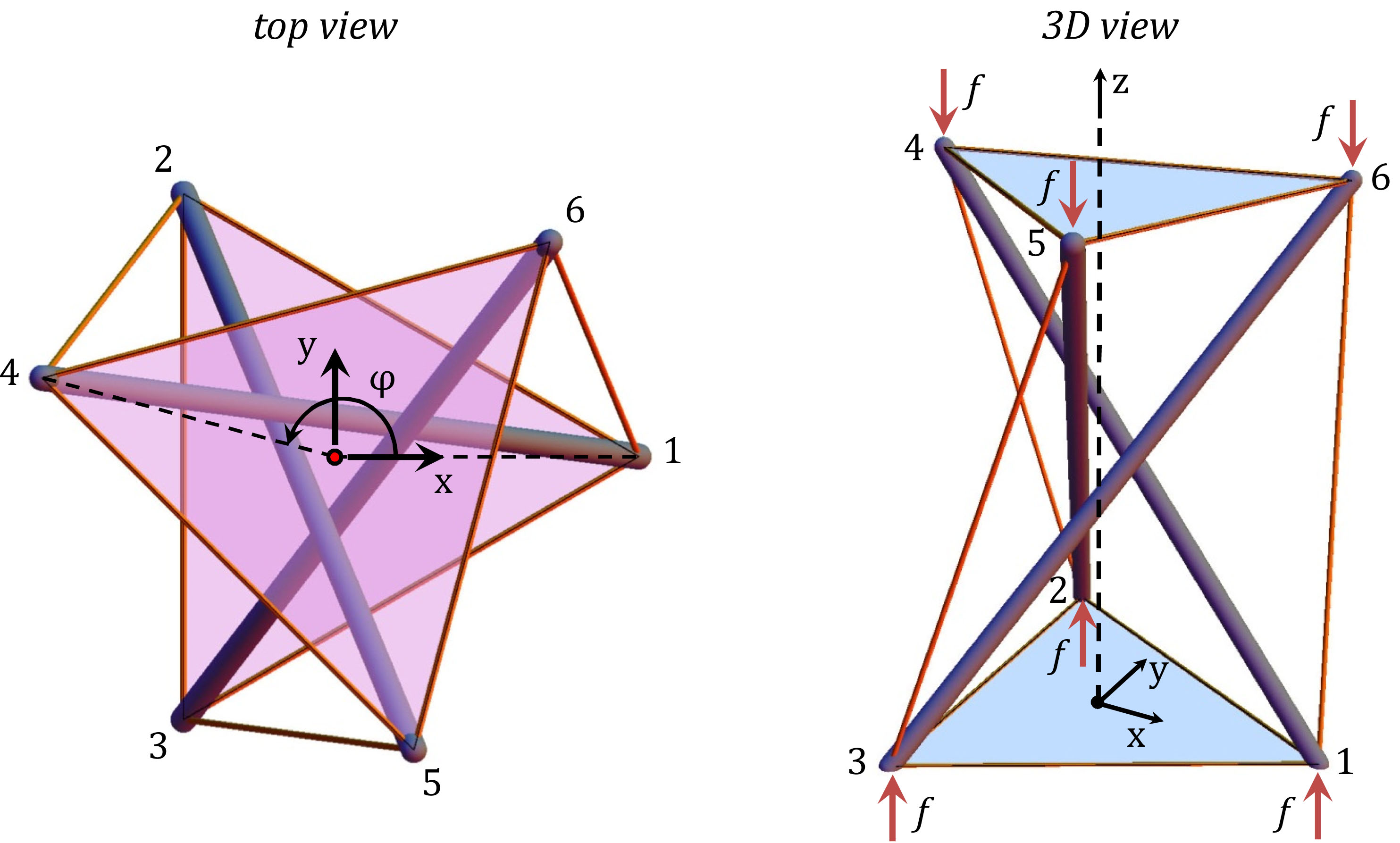
Figure 1: Reference configuration of a minimal regular tensegrity prism.

We assume that the prism is loaded in the $z$ direction by three equal forces (each of magnitude $f=F/3$) in correspondence with the bottom base $1,2,3$, and three forces of equal magnitude but opposite direction in correspondence with the top base $4,5,6$ (Fig. 1). Under such a uniform axial loading, it is easy to recognize that the deformation of the prism maintains its top and bottom bases parallel to each other, and simultaneously changes the angle of twist $\varphi$ and the height $h$. The geometrically feasible configurations are obtained by letting $\varphi$ vary between $\varphi=-\pi/3$ (cross-strings touching each other), and $\varphi=\pi$ (bars touching each other), as shown in Fig. 2. Hereafter, we refer to the configuration with the bars touching each other as the ‘locking’ configuration of the prism. Let us consider the equilibrium equations associated with an arbitrary node of the prism, which set to zero the summation of all the forces acting on the given node in the current configuration. It is an easy task to show that such equations can be written as it follows

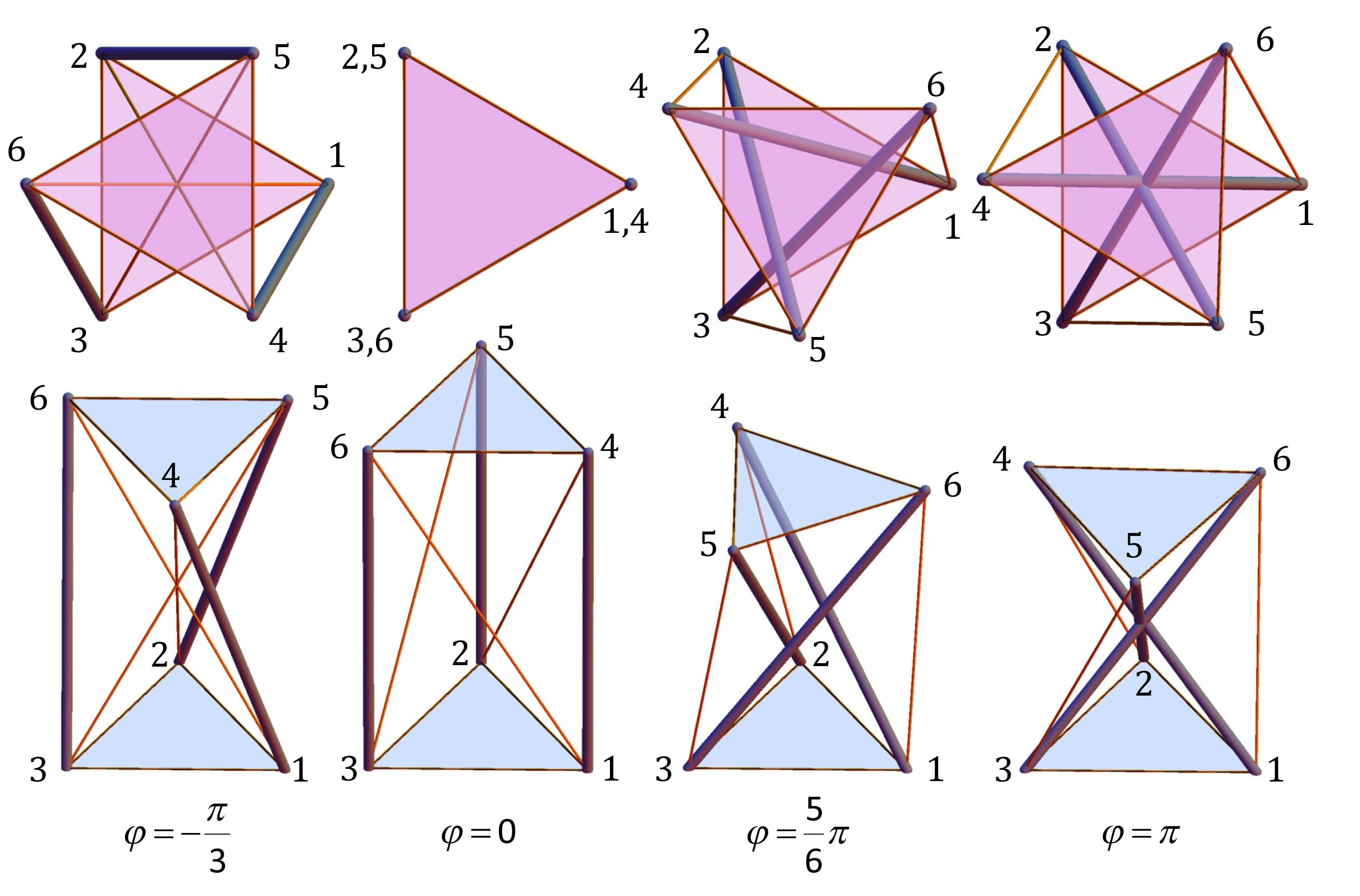
Figure 2: Sequence of configurations corresponding to feasible values of the twisting angle $\varphi$.

$$\frac{1}{6}\ell\left(2\sqrt{3}(x_{1}+3x_{2}-x_{3})+\sqrt{3}(x_{1}+2x_{3})\cos(\varphi)-3x_{1}\sin(\varphi)\right) = 0$$

$$\frac{1}{6}\ell\left(\sqrt{3}(x_{1}+2x_{3})\sin(\varphi)+3x_{1}\cos(\varphi)\right) = 0$$ (35)

$$h(x_{3}-x_{1})-\frac{F}{3} = 0$$

where $x_{1}$, $x_{2}$ and $x_{3}$ are the forces per unit length (i.e, the force densities) acting in the cross-string, base-strings, and bar attached to the current node, respectively. Such force densities are assumed positive if the strings are stretched, and the bars are compressed. We say that the prism occupies a proper tensegrity placement if one has: $x_{1}\geq 0,x_{2}\geq 0$ (i.e., the strings are either in tension or, at most, slack). It is not difficult to verify that the system of equations (35) admits the following general solution

$$x_{1} = -\frac{2F\sin(\varphi)}{3\sqrt{3}h\left(\sqrt{3}\sin(\varphi)+\cos(\varphi)\right)}$$

$$x_{2} = -\frac{F\left(\sin^{2}(\varphi)-\sqrt{3}\sin(\varphi)+\cos^{2}(\varphi)-\cos(\varphi)\right)}{9h\left(\sqrt{3}\sin(\varphi)+\cos(\varphi)\right)}$$ (36)

$$x_{3} = \frac{F}{3h}-\frac{2F\sin(\varphi)}{3\sqrt{3}h\left(\sqrt{3}\sin(\varphi)+\cos(\varphi)\right)}$$

Restricting our attention to the geometrically feasible configurations ($\varphi\in[-\pi/3,\pi]$), we note that the solution (36) becomes indeterminate when either $\varphi=-\pi/6$, or $\varphi=5\pi/6$, that is, when the quantity $\sqrt{3}\sin(\varphi)+\cos(\varphi)$ is zero. This means that the configurations corresponding to such values of $\varphi$ may exhibit nontrivial states of self-stress, i.e., nonzero force densities in the prism members for $F=0$ (prestressable configurations). By solving the first two equations (35) for $x_{2}$ and $x_{3}$, we characterize the self-stress states of the prism by

$$\varphi=-\frac{\pi}{6}: x_{2}=-\frac{x_{1}}{\sqrt{3}}, x_{3}=x_{1}$$ (37)

$$\varphi=\frac{5}{6}\pi: x_{2}=\frac{x_{1}}{\sqrt{3}}, x_{3}=x_{1}$$ (38)

for arbitrary $x_{1}$. Eqs. (37) and (38) show that a nontrivial state of self-stress compatible with an effective tensegrity placement is possible only for $\varphi=5\pi/6$. As a matter of fact, Eq. (37) highlights that $x_{1}$ and $x_{2}$ have opposite signs for $\varphi=-\pi/6$, which implies that the prism is either unstressed ($x_{1}=x_{2}=x_{3}=0$), or has some strings stretched and the others compressed in such a configuration. In contrast, Eq. (38) reveals that $x_{1}$ and $x_{2}$ have equal signs for $\varphi=5\pi/6$. The prism is loaded in compression for $\theta>0$, and in tension for $\theta<0$, where $\theta=\varphi-5\pi/6$ (cf. Section 3, and Oppenheim and Williams, (2000); Fraternali et al., (2012)). By manipulating Eqs. (32) and (36), we detect that all the cross strings are vertical and carry force densities $x_{1}=f/h$, for $\varphi=2/3\pi$ ($\theta=-\pi/6$). In the same configuration, the base strings and the bars carry zero forces ($x_{2}=x_{3}=0$). We take as a reference the configuration of the prism such that $\varphi=\varphi_{0}=5\pi/6$, and let $s_{0}$, $\ell_{0}$ and $b_{0}$ denote the lengths of the cross-strings, base-strings and bars in such a configuration, respectively. By inserting $\ell_{0}$ and $s_{0}$ into Eqs. (33) and (34), we can easily compute the reference values of the prism height and bar length as follows

$$h_{0} = \sqrt{s_{0}^{2}+\frac{1}{3}\left(\sqrt{3}-2\right)\ell_{0}^{2}},\ \ \ \ \ \ b_{0}\ =\ \sqrt{s_{0}^{2}+\frac{2\ell_{0}^{2}}{\sqrt{3}}}$$ (39)

2.1 Fully elastic model

A fully elastic model is obtained by describing all the prism members (bars and strings) as linear springs characterized by the following constitutive laws (Skelton and de Oliveira,, 2010)

$$x_{1} = \frac{1}{s}\ k_{1}\ (s-s_{N}),\ \ \ x_{2}\ =\ \frac{1}{\ell}\ k_{2}\ (\ell-\ell_{N}),\ \ \ x_{3}\ =\ -\ \frac{1}{b}\ k_{3}\ (b-b_{N})$$ (40)

where $k_{1}$, $k_{2}$ and $k_{3}$ are spring constants, and $s_{N}$, $\ell_{N}$ and $b_{N}$ are the rest lengths (or natural lengths) of cross-strings, base-strings and bars, respectively. Upon neglecting the change of the cross-section areas of all members during the prism deformation, we compute the spring constants as follows (Skelton and de Oliveira,, 2010)

$$k_{1} = \frac{E_{1}A_{1}}{s_{N}},\ \ \ k_{2}\ =\ \frac{E_{2}A_{2}}{\ell_{N}},\ \ \ k_{3}\ =\ \frac{E_{3}A_{3}}{b_{N}}$$ (41)

where $E_{1}$, $E_{2}$, $E_{3}$, and $A_{1}$, $A_{2}$, $A_{3}$ are the elastic moduli and the cross-section areas of the cross-strings, base-strings and bars, respectively.

2.1.1 Reference configuration

Hereafter, we assume that $\ell_{N}$ and $s_{N}$ are given, and that the cross-string prestrain is prescribed, i.e., the quantity

$$p_{0} ={(s_{0}-s_{N})}/{s_{N}}$$ (42)

In line with the above assumptions, we compute the reference length of the cross-strings ($s_{0}$), and the reference value of the force density in such members ($x_{1}^{(0)}$) through

$$s_{0} = {s_{N}}({1+p_{0}})$$ (43)

$$x_{1}^{(0)} = \frac{1}{s_{0}}\ k_{1}\ (s_{0}-s_{N})\ =\ \frac{A_{1}E_{1}}{s_{N}}\ \frac{p_{0}}{1+p_{0}},$$ (44)

Using (38), (40) and (44), we are led to the following reference values of the force densities in the base strings ($x_{2}^{(0)}$) and bars ($x_{3}^{(0)}$)

$$x_{2}^{(0)} = \frac{1}{\ell_{0}}\ k_{2}\ (\ell_{0}-\ell_{N})\ =\ \frac{A_{1}E_{1}}{\sqrt{3}s_{N}}\ \frac{p_{0}}{1+p_{0}}$$ (45)

$$x_{3}^{(0)} = -\ \frac{1}{b_{0}}\ k_{3}\ (b_{0}-b_{N})\ =\ \frac{A_{1}E_{1}}{s_{N}}\ \frac{p_{0}}{1+p_{0}}$$ (46)

Eq. (45) can be solved for $\ell_{0}$, yielding

$$\ell_{0} = \frac{3A_{2}E_{2}\left(p_{0}+1\right)s_{N}\ell_{N}}{p_{0}\left(3A_{2}E_{2}s_{N}-\sqrt{3}A_{1}E_{1}\ell_{N}\right)+3A_{2}E_{2}s_{N}}$$ (47)

On the other hand, the substitution of (43) and (47) into (39)₂ gives

$$b_{0} = \eta\ s_{0}\ =\ \eta\ \left(1+p_{0}\right)\ s_{N}$$ (48)

where

$$\eta = \sqrt{\frac{6\sqrt{3}A_{2}^{2}E_{2}^{2}\ell_{N}^{2}}{\left(p_{0}\left(3A_{2}E_{2}s_{N}-\sqrt{3}A_{1}E_{1}\ell_{N}\right)+3A_{2}E_{2}s_{N}\right){}^{2}}+1}$$ (49)

By solving Eq. (46) for $b_{N}$ and employing (48), we finally obtain

$$b_{N} = \frac{\eta A_{3}E_{3}}{A_{3}E_{3}-\eta A_{1}E_{1}}\ \left(1+p_{0}\right)\ s_{N}$$ (50)

2.1.2 The elastic problem

The substitution of Eqns. (40) into (35) leads us to the following elastic problem

$$g_{1} = \frac{1}{6}\ell\left(k_{3}\ 4\sin^{2}\left(\frac{\varphi}{2}\right)\left(\sqrt{3}-\frac{3b_{N}}{\sqrt{3h^{2}-2\ell^{2}\cos(\varphi)+2\ell^{2}}}\right)\right.$$ (51)

$$\ \ \ \ \ \ \left.+\ k_{1}\ \left(-3\sin(\varphi)+\sqrt{3}\cos(\varphi)+2\sqrt{3}\right)\ +\ k_{2}\ \frac{6\sqrt{3}\left(\ell-\ell_{N}\right)}{\ell}\right.$$

$$\ \ \ \ \ \ \left.-\ k_{1}\ \frac{3s_{N}\left(-\sqrt{3}\sin(\varphi)+\cos(\varphi)+2\right)}{\sqrt{3h^{2}-\sqrt{3}\ell^{2}\sin(\varphi)+\ell^{2}\cos(\varphi)+2\ell^{2}}}\right)\ =\ 0$$

$$g_{2} = \frac{1}{6}\ell\left(k_{3}\ 2\sin(\varphi)\left(\frac{3b_{N}}{\sqrt{3h^{2}-2\ell^{2}\cos(\varphi)+2\ell^{2}}}-\sqrt{3}\right)\right.$$ (52)

$$\ \ \ \ \ \ \left.+\ k_{1}\ \left(\sqrt{3}\sin(\varphi)+3\cos(\varphi)\right)\right.$$

$$\ \ \ \ \ \ \left.-\ k_{1}\ \frac{3s_{N}\left(\sin(\varphi)+\sqrt{3}\cos(\varphi)\right)}{\sqrt{3h^{2}-\sqrt{3}\ell^{2}\sin(\varphi)+\ell^{2}\cos(\varphi)+2\ell^{2}}}\right)\ =\ 0$$

$$g_{3} = -f\ +\ k_{3}\ h\left(\frac{b_{N}}{\sqrt{h^{2}-\frac{2}{3}\ell^{2}\cos(\varphi)+\frac{2\ell^{2}}{3}}}-1\right)$$ (53)

$$\ \ \ +\ k_{1}\ h\left(\frac{\sqrt{3}s_{N}}{\sqrt{3h^{2}-\sqrt{3}\ell^{2}\sin(\varphi)+\ell^{2}\cos(\varphi)+2\ell^{2}}}-1\right)\ =\ 0$$

2.1.3 Path-following method

We formulate a path-following approach to the nonlinear problem (51)–(53), by introducing the following ‘extended system’ (Riks,, 1984; Wriggers and Simo,, 1990; Fraternali et al.,, 2013)

$$\tilde{{\mathbf{g}}} = \left[\begin{array}[]{c}{\mathbf{g}}({\mathbf{v}},f)\\ \\ \psi({\mathbf{v}},f)\end{array}\right]=0$$ (57)

where we set ${\mathbf{v}}=[\ell,\varphi,h]^{T}$, ${\mathbf{g}}=[g_{1},g_{2},g_{3}]^{T}$, and let $\psi({{\mathbf{v}}},f)=0$ denote a constraint equation characterizing the given loading condition. In the case of a displacement control loading, we in particular assume

$$\psi = v_{k}-c=0,$$ (58)

letting $v_{k}$ coincide with $v_{1}\equiv\ell$ (base edge control); $v_{2}\equiv\varphi$ (twist control) or $v_{3}\equiv h$ (height control), and letting $c$ denote a given constant. The Newton–Raphson linearization of (57) at a given starting point ($\bar{\mathbf{v}}$, $\bar{f}$) leads us to the incremental problem

$$\begin{bmatrix}\nabla_{{\mathbf{v}}}{\mathbf{g}}&\nabla_{f}{\mathbf{g}}\\ \\ \nabla_{{\mathbf{v}}}\psi^{T}&\nabla_{f}\psi\\ \end{bmatrix}\begin{bmatrix}\Delta{\mathbf{v}}\\ \\ \Delta f\\ \end{bmatrix}=-\begin{bmatrix}{\bar{\mathbf{g}}}\\ \\ \bar{\psi}\end{bmatrix}$$ (59)

where we set ${\bar{\mathbf{g}}}={\mathbf{g}}(\bar{\mathbf{v}},\bar{f})$; ${\bar{\psi}}=\psi(\bar{\mathbf{v}},\bar{f})$; and

$$\nabla_{{\mathbf{v}}}{\mathbf{g}}=\begin{bmatrix}\frac{\partial g_{1}}{\partial v_{1}}&\frac{\partial g_{1}}{\partial v_{2}}&\frac{\partial g_{1}}{\partial v_{3}}\\ \\ \frac{\partial g_{2}}{\partial v_{1}}&\frac{\partial g_{2}}{\partial v_{2}}&\frac{\partial g_{2}}{\partial v_{3}}\\ \\ \frac{\partial g_{3}}{\partial v_{1}}&\frac{\partial g_{3}}{\partial v_{2}}&\frac{\partial g_{3}}{\partial v_{3}}\end{bmatrix},\ \ \nabla_{f}{\mathbf{g}}=\left[\begin{array}[]{c}\frac{\partial g_{1}}{\partial f}\\ \\ \frac{\partial g_{2}}{\partial f}\\ \\ \frac{\partial g_{3}}{\partial f}\end{array}\right],\ \ \nabla_{{\mathbf{v}}}\psi=\left[\begin{array}[]{c}\frac{\partial\Psi}{\partial{\mathbf{v}}_{1}}\\ \\ \frac{\partial\Psi}{\partial{\mathbf{v}}_{1}}\\ \\ \frac{\partial\Psi}{\partial{\mathbf{v}}_{1}}\end{array}\right]$$ (60)

We now introduce the notations ${\mathbf{V}}:=\nabla_{{\mathbf{v}}}{\mathbf{g}}$ and ${\mathbf{f}}:=\nabla_{f}{\mathbf{g}}=[0,0,-1]^{T}$, and assume that ${\mathbf{V}}$ is invertible at (${\mathbf{v}}=\bar{\mathbf{v}}$, $f=\bar{f}$). The incremental problem (59) is solved by first computing the partial solutions

$$\Delta{\mathbf{v}}_{f}\ =\ -{\mathbf{V}}^{-1}{\mathbf{f}}\ =\ \begin{bmatrix}V^{-1}_{13}\\ V^{-1}_{23}\\ V^{-1}_{33}\end{bmatrix},\ \ \ \ \ \Delta{\mathbf{v}}_{g}\ =\ -{\mathbf{V}}^{-1}\bar{{\mathbf{g}}},$$ (61)

and next the updates

$$\Delta{\mathbf{v}} = \Delta f\Delta{\mathbf{v}}_{f}+\Delta{\mathbf{v}}_{g},$$ (62)

$$\Delta f = -\ \frac{\bar{\psi}+\nabla_{{\mathbf{v}}}\psi\cdot\Delta{\mathbf{v}}_{g}}{\nabla_{f}\psi+\nabla_{{\mathbf{v}}}\psi\cdot\Delta{\mathbf{v}}_{f}}$$ (63)

Equations (62)–(63) lead us to the new predictor ($\bar{{\mathbf{v}}}$ + $\Delta{\mathbf{v}}$, $\bar{f}$ + $\Delta f$), which is used to reiterate the updates (62)–(63), until the residual $\left\|{\mathbf{g}}(\bar{{\mathbf{v}}},\bar{f})\right\|$ gets lower than a given tolerance. Once a new equilibrium point is obtained, the value of constant $c$ in Eqn. (58) is updated and the path-following procedure is continued. The explicit expression for the ${\mathbf{V}}$ matrix is given in Appendix.

Let us assume $\psi=h-{\bar{h}}$ (height control loading). By writing Eqn. (62) in correspondence with a solution of the extended system (57) (${\bar{\mathbf{g}}}=\mathbf{0}$, ${\bar{\psi}}=0$), we easily obtain $\Delta{\mathbf{v}}_{g}=0$, and

$$\begin{bmatrix}\Delta\ell\\ \Delta\varphi\\ \Delta h\end{bmatrix} = \Delta f\begin{bmatrix}V^{-1}_{13}\\ V^{-1}_{23}\\ V^{-1}_{33}\end{bmatrix}$$ (64)

which implies

$$\Delta h = {\Delta f}\ {V^{-1}_{33}}\ =\ \frac{\Delta F}{3}\ {V^{-1}_{33}}$$ (65)

Eqn. (65) shows that the axial stiffness $K_{h}^{el}$ of the fully elastic model is given by

$$K_{h}^{el}=-\frac{3}{V^{-1}_{33}}$$ (66)

The value of the above quantity at ${\mathbf{v}}={\mathbf{v}}_{0}=[\ell_{0},\varphi_{0},h_{0}]^{T}$ represents the axial stiffness $K_{0}^{el}$ of the prism in correspondence with the reference configuration, and it is not difficult to show that such a quantity is zero for $p_{0}=0$ (see the Appendix).

2.2 Rigid-elastic model

In a series of studies available in the literature, the mechanical response of tensegrity prisms has been analyzed by assuming that the bases and bars behave rigidly, while the cross strings respond as elastic springs (rigid-elastic model, cf., e.g., Oppenheim and Williams, (2000); Fraternali et al., (2012)). Such a modeling keeps $b$ and $\ell$ fixed ($b=b_{0}=\mbox{const}$, $\ell=\ell_{0}=\mbox{const}$), and relates $h$ to $\varphi$ through Eq. (33). Let us solve Eq. (33) for $h$, obtaining the equation

$$h = \sqrt{b^{2}\ -\ \frac{2}{3}\ell^{2}(1-\cos\varphi)}$$ (67)

which, once inverted (for $-\pi/3\leq\varphi\leq\pi$), gives

$$\varphi = \arccos{\left(1-\frac{b^{2}-h^{2}}{2a^{2}}\right)}$$ (68)

where $a=\ell/\sqrt{3}$ denoted the radius of the circumference circumscribed to the base triangles. The response of the rigid–elastic model is easily modeled by substituting (40)₁ into the equilibrium equations (35), and solving the resulting system of algebraic equations with respect to $F$, $x_{2}$, and $x_{3}$, for given $h$ (or $\varphi$). It is not difficult to verify that such an approach leads to the same constitutive law given in Oppenheim and Williams, (2000); Fraternali et al., (2012), that is

$${F} = 3k_{1}\ (s-s_{N})\ \frac{h}{2s}\ \left(3+\frac{\sqrt{3}\left(2a^{2}+h^{2}-b^{2}\right)}{a^{2}\sqrt{-\frac{\left(h^{2}-b^{2}\right)\left(4a^{2}+h^{2}-b^{2}\right)}{a^{4}}}}\right)$$ (69)

$$= \frac{k_{1}\csc(\varphi)\left(3\sin(\varphi)+\sqrt{3}\cos(\varphi)\right)\sqrt{3b^{2}+2\ell^{2}\cos(\varphi)-2\ell^{2}}}{2\sqrt{3b^{2}-\sqrt{3}\ell^{2}\sin(\varphi)+3\ell^{2}\cos(\varphi)}}$$

$$\times\ \left(\sqrt{9b^{2}-3\sqrt{3}\ell^{2}\sin(\varphi)+9\ell^{2}\cos(\varphi)}-3s_{N}\right)$$

It is also easily shown that the rigid–elastic model predicts an infinitely stiff response ($F\rightarrow\infty$) for $\varphi\rightarrow\pi$ (assuming $b>2a$). Once $h$ (or $\varphi$) is given, $x_{1}$ is computed through (40)₁ and (34); ${F}$ is computed through (69); and $x_{2}$ and $x_{3}$ are obtained from the equilibrium equations (35). The differentiation of (69) with respect to $h$ gives the tangent axial stiffness of the present model (cf. the Appendix). The reference value of such a quantity ($\varphi=5/6\pi$) is given by

$$K_{h_{0}}^{rigel} = -{F}^{{}^{\prime}}(h=h_{0})\ =\ 12\ \sqrt{3}\ k_{1}\frac{p_{0}}{1+p_{0}}\ \left(\frac{h_{0}}{a}\right)^{2}$$ (70)

and it is immediately seen that also $K_{0}^{rigel}$ is zero for $p_{0}=0$, as well as $K_{0}^{el}$.

3 Numerical results

The current section presents a collection of numerical results aimed to illustrate the main features of the mechanical models presented in Section 2. We examine the mechanical response of tensegrity prisms having the same features as the physical models studied in Amendola et al., (2014). Such prisms are equipped with M8 threaded bars made out of white zinc plated grade 8.8 steel (DIN 976-1), and strings consisting of PowerPro^® braided Spectra^® fibers with 0.76 mm diameter (commercialized by Shimano American Corporation - Irvine CA). The properties of the employed materials are shown in Table 1. Let ${\bar{A}}_{1}$, ${\bar{A}}_{2}$, ${\bar{A}}_{3}$ and ${\bar{E}}_{1}$, ${\bar{E}}_{2}$, ${\bar{E}}_{3}$ denote the cross-sectional areas and elastic moduli of the strings and bars defined according to Table 1. In order to study the transition from the elastic to the rigid–elastic model, we hereafter study the mechanical response of elastic prisms endowed with the following spring constants (cf. Section 2.1).

$$k_{1} = \frac{{\bar{E}}_{1}{\bar{A}}_{1}}{s_{N}},\ \ \ k_{2}\ =\ \alpha\ \frac{{\bar{E}}_{2}{\bar{A}}_{2}}{\ell_{N}},\ \ \ k_{3}\ =\ \beta\ \frac{{\bar{E}}_{3}{\bar{A}}_{3}}{b_{N}}$$ (71)

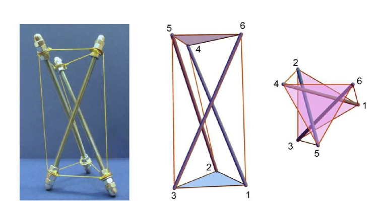
Figure 9: Slender prism model. Left: photograph of a real-scale example (Amendola et al.,, 2014). Center and right: 3D view (center) and top view (right) of the theoretical model.

where $\alpha$ and $\beta$ are rigidity multipliers ranging within the interval $[1,\infty]$. The case of $\alpha=\beta=1$ corresponds to the fully elastic (‘el’) model of Sect. 2.1.2, while the limiting case with $\alpha=\beta\rightarrow\infty$ corresponds to the rigid–elastic (‘rigel’) model presented in Sect. 2.2. The equilibrium configurations of the elastic prism model are numerically determined through the path-following method given in Section 2.1.3, letting the angle of twist $\varphi$ to vary within the interval $[2/3\pi,\pi)$, which corresponds to effective tensegrity placements of the structure (cf. Section 2). We examine a large variety of prestrains $p_{0}$, and both thick and slender reference configurations (cf. Figs. 3 and 9, respectively). Let $\delta=h_{0}-h$ denote the axial displacement of the prism from the reference configuration, and let $\varepsilon=\delta/h_{0}$ denote the corresponding axial strain (positive when the prism is compressed). We name stiffening a branch of the $F-\delta$ response showing axial stiffness $K_{h}$ increasing with $|\delta|$ (or $|\varepsilon|$), and softening a branch that instead shows $K_{h}$ decreasing with $|\delta|$ ($|\varepsilon|$). The axial forces carried by the cross-strings, base-strings, and bars are denoted by $N_{1}$, $N_{2}$, and $N_{3}$, respectively. We assume that $N_{1}$ and $N_{2}$ are positive in tension, and that $N_{3}$ is instead positive in compression.

Property	bars	strings
area (mm2)	36.6	0.45
mass density (kg/m3)	7850	793
elastic modulus (GPa)	203.53	5.48

Table 1: Properties of the materials employed in the numerical simulations.

3.1 Thick prisms

We examine ‘thick’ prisms featuring: $s_{N}=0.08$ m, $\ell_{N}=0.132$ m, and reference lengths $s_{0}$, $\ell_{0}$, $b_{0}$, and $h_{0}$ variable with the cross string prestrain $p_{0}$ (cf. Section 2.1.1). Table 2 shows noticeable values of such variables and $K_{h_{0}}$, for different prestrains $p_{0}$; the fully elastic model; and the rigid–elastic model. It is seen that $h_{0}$ is always smaller than $\ell_{0}$ in the present case, which justifies the name ‘thick’ given to the prisms under consideration. The difference between $K_{h_{0}}^{el}$ and $K_{h_{0}}^{rigel}$ grows with the prestrain $p_{0}$, being zero for $p_{0}=0$ ($K_{h_{0}}^{el}=K_{h_{0}}^{rigel}=0$). Fig. 4 shows the force $F$ vs. $\delta$ curves of the ‘el’ samples for different values of $p_{0}$. Fig. 5 provides the same curves for different values of the stiffness multipliers $\alpha$ and $\beta$, and $p_{0}=0.1$. Finally, Figs. 6 and 7 illustrate the variations with the angle of twist $\varphi$ of the axial stiffness $K_{h}$; the prism height $h$; and the axial forces $N_{1}$, $N_{2}$ and $N_{3}$. In the ‘el’ case, the results in Figs. 4 and 6 highlight that the compressive response for $p_{0}\leq 0.005$ initially features a stiffening branch, next a softening branch, and finally an unstable phase (strain softening: $F$ decreasing with $\delta$), as the axial strain $\varepsilon$ increases. When $p_{0}$ grows above 0.005, the initial stiffening branch disappears, and the compressive response is always softening. The final unstable branch is associated with the snap buckling of the prism to the completely collapsed configuration featuring zero height $h$ (cf. Fig. 8). Such a collapse event can fully take place when $p_{0}\geq 0.05$, but is instead prevented by prism locking for lower values of $p_{0}$ (Figs. 4 and 6). It is worth noting that the maximum compression displacement $\delta^{max}$ of the current prism model increases with $p_{0}$. Overall, we conclude that the compressive response of the thick prism is markedly different from that of the rigid–elastic model analyzed in Oppenheim and Williams, (2000); Fraternali et al., (2012), since the latter predicts an infinitely stiff response for $\delta\rightarrow\delta^{max}$. For what concerns the tensile response, we observe that the ‘el’ model is always stiffening in tension, for any $p_{0}\in[0,0.4]$ (Figs. 4, 6). We also observe that the minimum axial displacement $\delta^{min}$ (i.e. the value of $\delta$ for $\varphi=2/3\pi$) grows in magnitude with $p_{0}$.

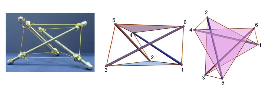
Figure 3: Thick prism model. Left: photograph of a real-scale example (Amendola et al.,, 2014). Center and right: 3D view (center) and top view (right) of the theoretical model.

$\alpha$=$\beta$	$p_{0}$	$s_{N}$ (m)	$s_{0}$ (m)	$\ell_{N}$ (m)	$\ell_{0}$ (m)	$b_{N}$ (m)	$b_{0}$ (m)	$h_{0}$ (m)	$K_{h_{0}}$ (N/m)
1	0	0.080	0.0800	0.1320	0.1320	0.1628	0.1628	0.0696	0
1	0.005	0.080	0.0804	0.1320	0.1326	0.1636	0.1636	0.0700	2595
1	0.1	0.080	0.0880	0.1320	0.1445	0.1785	0.1785	0.0767	29720
1	0.2	0.080	0.0960	0.1320	0.1569	0.1941	0.1940	0.0838	39257
1	0.3	0.080	0.1040	0.1320	0.1692	0.2095	0.2095	0.0909	42601
1	0.4	0.080	0.1120	0.1320	0.1814	0.2248	0.2248	0.0980	43465
$\rightarrow\infty$	0	0.080	0.0800	0.1320	0.1320	0.1628	0.1628	0.0696	0
$\rightarrow\infty$	0.005	0.080	0.0804	0.1320	0.1320	0.1630	0.1630	0.0701	2682
$\rightarrow\infty$	0.1	0.080	0.0880	0.1320	0.1320	0.1669	0.1669	0.0787	49582
$\rightarrow\infty$	0.2	0.080	0.0960	0.1320	0.1320	0.1713	0.1713	0.0875	92033
$\rightarrow\infty$	0.3	0.080	0.1040	0.1320	0.1320	0.1759	0.1759	0.0962	129005
$\rightarrow\infty$	0.4	0.080	0.1120	0.1320	0.1320	0.1807	0.1807	0.1048	161679

Table 2: Geometric variables and initial axial stiffness $K_{h_{0}}$ of the thick prism model, for different values of the cross-string prestrain $p_{0}$; the fully elastic model ($\alpha=\beta=1$); and the rigid–elastic model ($\alpha=\beta\rightarrow+\infty$).

Figure 4: $F$–$\delta$ curves of the thick prism model, when loaded in compression (top), and tension (bottom), for $\alpha=\beta=1$ and different values of $p_{0}$.

Let us now pass to studying the response of thick prisms for different values of the rigidity multipliers $\alpha$ and $\beta$. The $F-\delta$ curves in Fig. 5 show that the response in compression of the thick prisms analyzed in this study switches from extremely soft to extremely stiff when $\alpha$ and $\beta$ grow from 1 (‘el’ model) to $+\infty$ (‘rigel’ model). In particular, we observe that $\alpha$ (i.e., the base rigidity) plays a more substantial role in the mechanical response of such a structure than does $\beta$ (the bar rigidity multiplier). We indeed note that the $F-\delta$ curves for $\alpha=\beta=10$ and $\alpha=\beta=100$ are not much different from those corresponding to $\alpha=10,\ \beta=1$ and $\alpha=100,\ \beta=1$, respectively. This is due to the fact that the axial stiffness of the bars is much higher than the axial stiffness of the strings (cf. Table 1), which implies that the assumption of bar rigidity is more realistic than the assumption of base rigidity, in the present case. When $p_{0}=0.005$, Fig. 7 shows that the response in tension of thick prisms is always stiffening, for all the examined values of $\alpha$ and $\beta$. In contrast, for $p_{0}=0.4$ we observe that such a response progressively switches from stiffening to softening, as $\alpha$ and $\beta$ grow to infinity (Fig. 7). Overall, we note that the stroke of the prism ($\delta^{max}-\delta^{min}$) decreases with $\alpha$ and $\beta$ (Fig. 5), and increases with $p_{0}$ (Fig. 4). Conversely, the value of $K_{h}$ at $\delta=\delta^{max}$ increases with $\alpha$ and $\beta$ (Fig. 7), and decreases with $p_{0}$ (Fig. 6).

Figure 5: $F$–$\delta$ curves of the thick prism model, when loaded in compression (top), and tension (bottom), for $p_{0}$ = 0.1 and different values of $\alpha$ and $\beta$.

Figure 6: $K_{h}$ vs. $\varphi$, $h$ vs. $\varphi$, and $N_{1},N_{2},N_{3}$ vs. $\varphi$ curves of the thick prism model for $\alpha$ = $\beta$ = 1, and different values of $p_{0}$.

The results in Fig. 6 highlight that the softening and unstable phases of the ‘el’ model are associated with a progressive decrease of the force acting in the cross-strings ($N_{1}$). The decrease of $N_{1}$ with $\varphi$ for $\alpha=\beta=1$ is confirmed by the results given in Fig 7, which show that the cross-strings tend to become slack as $\varphi$ approaches $\pi$ ($\delta\rightarrow\delta^{max}$), in the ‘el’ case. The $N_{2}$ vs. $\varphi$ curves of the base-strings highlight that $N_{2}$ grows monotonically with $\varphi$ (starting with the value $N_{2}=0$ at $\varphi=2/3\pi$), independently of $p_{0}$, $\alpha$ and $\beta$ (Figs. 6 and 7). In particular, the rate of growth of $N_{2}$ decreases with $p_{0}$, and increases with $\alpha$ and $\beta$, tending to infinity for $\varphi\rightarrow\pi$ ($\delta\rightarrow\delta^{max}$), when $\alpha=\beta\rightarrow\infty$. This implies that, in real life, the base strings would yield before reaching the ‘locking’ configuration, in the ‘rigel’ limit. The axial force response of the bars resembles that of the base strings, and we note that the bars tend to buckle before reaching the locking configuration in the‘rigel’ limit. For $p_{0}\geq 0.05$, it is worth noting that the maximum value of $\varphi$ is less than $\pi$ (cf. Figs. 6, 7), since in such cases the axial collapse precedes the locking configuration $\varphi=\pi$.

Figure 7: $K_{h}$ vs. $\varphi$ and $N_{1},N_{2},N_{3}$ vs. $\varphi$ curves of the thick prism model for $p_{0}$ = 0.005 (left), $p_{0}$ = 0.4 (right), and different values of $\alpha$ and $\beta$.

Figure 8: Member forces (kN) in different configurations of the thick prism, for $\alpha$ = $\beta$ = 1, and $p_{0}$ = 0.05.

3.2 Slender prisms

The ‘slender’ prisms analyzed in the present study feature: $s_{N}=0.162$ m, $\ell_{N}=0.08$ m, and equilibrium height $h_{0}$ about twice the base side $\ell_{0}$ (cf. Table 3). Figs. 10 and 11 show the force $F$ vs. $\delta$ curves of such prisms for different values of $p_{0}$, $\alpha$ and $\beta$, while Figs. 12 and 13 provide the curves relating the axial stiffness $K_{h}$, the prism height $h$, and the axial forces $N_{1}$, $N_{2}$, $N_{3}$ with the angle of twist $\varphi$. Some snapshots of the deformation of the slender prism for $\varphi\in[2/3\pi,\pi]$; $\alpha$ = $\beta$ = 1; $p_{0}$ = 0.05; and $p_{0}$ = 0.4 are illustrated in Figs. 14 and 15.

$\alpha$=$\beta$	$p_{0}$	$s_{N}$ (m)	$s_{0}$ (m)	$\ell_{N}$ (m)	$\ell_{0}$ (m)	$b_{N}$ (m)	$b_{0}$ (m)	$h_{0}$ (m)	$K_{h_{0}}$ (N/m)
1	0	0.1620	0.1620	0.080	0.0800	0.1834	0.1834	0.1602	0.0
1	0.005	0.1620	0.1628	0.080	0.0801	0.1842	0.1842	0.1610	18552
1	0.02	0.1620	0.1652	0.080	0.0804	0.1865	0.1865	0.1635	67597
1	0.05	0.1620	0.1701	0.080	0.0811	0.1911	0.1911	0.1684	144450
1	0.1	0.1620	0.1782	0.080	0.0821	0.1989	0.1989	0.1765	236357
1	0.2	0.1620	0.1944	0.080	0.0840	0.2143	0.2143	0.1928	360901
1	0.3	0.1620	0.2106	0.080	0.0856	0.2299	0.2299	0.2090	454877
1	0.4	0.1620	0.2268	0.080	0.0871	0.2454	0.2454	0.2253	537673
$\rightarrow\infty$	0	0.1620	0.1620	0.080	0.080	0.1834	0.1834	0.1602	0.0
$\rightarrow\infty$	0.005	0.1620	0.1628	0.080	0.080	0.1841	0.1841	0.1610	19235
$\rightarrow\infty$	0.02	0.1620	0.1652	0.080	0.080	0.1863	0.1863	0.1635	77745
$\rightarrow\infty$	0.05	0.1620	0.1701	0.080	0.080	0.1906	0.1906	0.1684	196369
$\rightarrow\infty$	0.1	0.1620	0.1782	0.080	0.080	0.1979	0.1979	0.1766	401754
$\rightarrow\infty$	0.2	0.1620	0.1944	0.080	0.080	0.2126	0.2126	0.1929	840075
$\rightarrow\infty$	0.3	0.1620	0.2106	0.080	0.080	0.2275	0.2275	0.2092	1315781
$\rightarrow\infty$	0.4	0.1620	0.2268	0.080	0.080	0.2425	0.2425	0.2255	1829454

Table 3: Geometric variables and initial axial stiffness $K_{h_{0}}$ of the slender prism model for different values of the cross-string prestrain $p_{0}$; the fully elastic model ($\alpha=\beta=1$); and the rigid–elastic model ($\alpha=\beta\rightarrow+\infty$).

Figure 10: $F$–$\delta$ curves of the slender prism model, when loaded in compression (top), and tension (bottom), for $\alpha=\beta=1$ and different values of $p_{0}$.

In the ‘el’ model with $p_{0}\leq 0.3$, we observe that the compressive response first shows a stiffening branch, and next a softening branch (cf. Figs. 10, 12, and 14). For $p_{0}=0.4$, the compressive branch of the $F$ vs. $\delta$ (or $F$ vs. $\varphi$) response is instead always softening, and terminates with an unstable phase (Figs. 10, 12, 15). Figs. 10 and 12 show that the tensile response of slender prisms is slightly softening for $p_{0}\geq 0.1$. In contrast, for $p_{0}\leq 0.05$ the same response is instead slightly stiffening. It is worth noting that the above behaviors are markedly different from those exhibited by the thick prisms analyzed in Section 3, since the latter feature unstable response in compression under low prestrains $p_{0}$, and always stiffening response in tension (Figs. 4, 6, 8). We now pass to examining the axial response of slender prisms for different values of the stiffness multipliers $\alpha$ and $\beta$, and $p_{0}=0.1$. Fig. 11 shows that the compressive response for $p_{0}=0.1$ is almost linear when $\delta\rightarrow\delta^{max}$ in the ‘el’ case, and tends to get infinitely stiff in the ‘rigel’ limit. The tensile response is instead less sensitive to $\alpha$ and $\beta$, and always softening (Fig. 11). The individual responses of the prism members highlight that the softening response in compression is always associated with decreasing values of the force carried by the cross-strings (cf. Figs. 12 and 13), as in the case of the thick prisms examined in the previous section. The deformations graphically illustrated in Fig. 15 highlight a marked stretching of the base-strings, in proximity to the locking configuration $\varphi=\pi$, when there results $\alpha$ = $\beta$ = 1, and $p_{0}$ = 0.4.

Figure 11: $F$–$\delta$ curves of the slender prism model, when loaded in compression (top), and tension (bottom), for $p_{0}$ = 0.1 and different values of $\alpha$ and $\beta$.

Figure 12: $K_{h}$ vs. $\varphi$, $h$ vs. $\varphi$ and $N_{1},N_{2},N_{3}$ vs. $\varphi$ curves of the slender prism model for $\alpha$ = $\beta$ = 1, and different values of $p_{0}$.

Figure 13: $K_{h}$ vs. $\varphi$ and $N_{1},N_{2},N_{3}$ vs. $\varphi$ curves of the slender prism model for $p_{0}$ = 0.005 (left), $p_{0}$ = 0.4 (right) and different values of $\alpha$ and $\beta$.

Figure 14: Member forces (kN) in different configurations of the slender prism, for $\alpha$ = $\beta$ = 1, and $p_{0}$ = 0.05.

Figure 15: Member forces (kN) in different configurations of the slender prism, for $\alpha$ = $\beta$ = 1, and $p_{0}$ = 0.4.

4 Experimental validation

The present section deals with an experimental validation of the models presented in Sections 2 and 3, against the results of quasi-static compression tests on physical prism samples (Amendola et al.,, 2014) (cf. also Section 3). We first examine the experimental responses of the thick prism specimens described in Table 4, where $N_{1}^{(0)}$ denotes the axial force carried by the cross-strings in correspondence with the reference configuration. Fig. 16 compares the theoretical (‘th-el’) and experimental (‘exp-el’) $F-\delta$ responses of such specimens, highlighting an overall good agreement between theory and experiments. We note a more compliant character of the experimental responses, as compared to those predicted by the fully-elastic model presented in Section 2, and oscillations of the experimental measurements. Such theory vs. experiment mismatches are explained by signal noise; progressive damage to the nodes during loading; string damage due to the rubbing of Spectra^® fibers against the rivets placed at the nodes; and geometric imperfections (refer to Amendola et al., (2014) for detailed descriptions of such phenomena). In particular, geometric imperfections arising in the assembly phase prevent the three bars of the current prisms from simultaneously coming into contact with each other when the angle of twist approaches $\pi$. The marker $\oslash$ in Fig. 16 indicates the first configuration at which two bars touch each other, while the marker $\otimes$ indicates the first configuration with all three bars interfering. It is worth noting that the full locking configuration (‘$\otimes$’) occurs at an angle of twist $\varphi$ appreciably lower than $\pi$, due to geometric imperfections and the nonzero thickness of the bars. Both the theoretical and experimental results shown in Fig. 16 indicate a clear softening character of the compressive response of the examined thick prisms.

type	$p_{0}$	$s_{N}$ (m)	$s_{0}$ (m)	$N_{1}^{(0)}$(N)	$\ell_{N}$ (m)	$\ell_{0}$ (m)	$b_{0}$ (m)
el	0.01	0.080	0.081	30.9	0.132	0.134	0.165
el	0.03	0.080	0.083	78.2	0.132	0.136	0.168
el	0.07	0.080	0.085	170.0	0.132	0.140	0.174

Table 4: Geometric and mechanical properties of thick prism samples.

Figure 16: Comparison of the theoretical and experimental responses of thick prisms with deformable bases.

We now pass to examining the experimental response of the slender prism models described in Table 5, which include two samples with deformable bases (‘el’ samples), and two samples aimed at reproducing the rigid–elastic model presented in Section 2.2 (‘rigel’ samples). The latter were assembled by replacing the base-strings of the ‘el’ systems with 12 mm thick aluminum plates (cf. Fig. 17, and Amendola et al., (2014)). Fig. 18 illustrates a comparison between the theoretical and experimental responses of the ‘el’ samples, which shows a rather good match between theory and experiment. In the present case, we observe reduced signal noise, as compared to the case of thick prisms, and all the bars getting simultaneously in touch at locking. The main mismatch between the theoretical and experimental responses shown in Fig. 18 consists of an anticipated occurrence of prism locking in the physical models, which has already been observed and discussed in the case of the thick specimens. It is interesting to note that both the theoretical and the experimental results shown in Fig. 18 indicate a slightly stiffening behavior of the ‘el’ samples with a ‘slender’ aspect ratio.

The final experimental results presented in Fig. 19 are aimed at validating the rigid–elastic model presented in Section 2.2 (‘rigel’ samples). One observes that the specimens endowed with nearly infinitely rigid bases feature a markedly stiff response in the proximity of the locking configuration, in line with the model presented in Oppenheim and Williams, (2000). We observe a more compliant character of the experimental $F-\delta$ curves of ‘rigel’ samples, as compared to the theoretical counterparts, which is explained by the not perfectly rigid behavior of the bases and the bars (physical samples), and the partial unthreading of the cross-strings from the lock washers placed at the the nodes (Amendola et al.,, 2014). The latter is induced by large tensile forces in the horizontal strings, when the system gets close to the locking configuration (cf. the theoretical results shown in Fig. 13, for $\alpha=\beta\rightarrow\infty$).

type	$p_{0}$	$s_{N}$ (m)	$s_{0}$ (m)	$N_{1}^{(0)}$(N)	$\ell_{N}$ (m)	$\ell_{0}$ (m)	$b_{0}$ (m)
el	0.07	0.162	0.173	165.9	0.080	0.081	0.194
el	0.09	0.162	0.176	219.9	0.080	0.082	0.197
rigel	0.06	0.162	0.172	150.0	0.080	0.080	0.192
rigel	0.11	0.162	0.181	286.0	0.080	0.080	0.200

Table 5: Geometric and mechanical properties of slender prism samples.

Figure 17: Photograph of a real-scale example of a slender prism endowed with thick aluminum bases (Amendola et al.,, 2014).

Figure 18: Comparison of the theoretical and experimental responses of slender prisms with deformable bases.

Figure 19: Comparison of the theoretical and experimental responses of slender prisms with rigid bases.

5 Concluding remarks

We have presented a fully elastic model of axially loaded tensegrity prisms, which generalizes previous models available in the literature (Oppenheim and Williams,, 2000; Fraternali et al.,, 2012). The mechanical theory presented in Section 2.1 assumes that all the elements of a tensegrity prism respond as elastic springs, and relaxes the rigidity constraints introduced in Oppenheim and Williams, (2000). On adopting the equilibrium approach to tensegrity systems described in Skelton and de Oliveira, (2010), we have written the equilibrium equations in the current configuration, thus developng a geometrical nonlinear model allowing for large displacements (Section 2.1). In addition, we have presented an incremental formulation of the equilibrium problem of axially loaded tensegrity prisms, which is particularly useful when using Netwon’s iterative schemes in numerical simulations (Section 2.1.3).

The numerical results presented in Section 3 highlight a rich variety of behaviors of tensegrity prisms under uniform axial loading and large displacements. The variegate mechanical response of such structures includes both extremely soft and markedly stiff deformation modes, depending on the geometry of the structure, the mechanical properties of the constituent elements, the magnitude of the cross-string prestrain $p_{0}$ (characterizing the whole state of self-stress), and the loading level (deformation-dependent behavior). We have found that ‘thick’ prisms exhibit softening response in compression under relatively low prestrains, and, on the contrary, stiffening response in tension over a large window of $p_{0}$ values (Figs. 4, 6, 8). The softening response in compression of such structures is often associated with a snap buckling event, which might lead the prism to axial collapse (prism height tending to zero). In contrast, we have noted that ‘slender’ prisms need large cable prestrains to show softening response in compression, and relatively low prestrains in order to feature softening response in tension (Fig. 10, 12, 14, 15). By letting the base and bar rigidities tend to infinity, we have numerically observed that the compressive response of thick and slender prisms progressively switches to infinitely stiff in the proximity of the locking configuration (Figs. 5, 7, 11, 13). In the rigid-elastic limit we have also noted that thick prisms exhibit stiffening response in tension (with the exception of cases characterized by extremely high values of $p_{0}$, cf. Fig. 7), while slender prisms instead typically feature slightly softening response in tension (cf. Figs. 11 and 13). An experimental validation of the mechanical models presented in Section 2 has been conducted against the results of quasi-static compression tests on physical samples (Amendola et al.,, 2014), with good agreement between theory and experiments. The given experimental results have confirmed the switching from softening to stiffening of the compressive response of the tested samples, in relation to the prism aspect ratio, the magnitude of the applied prestress, and the rigidity of the terminal bases.

The outcomes of the present study significantly enlarge the known spectrum of behavior of tensegrity prisms under axial loading, as compared to the literature to date (Oppenheim and Williams,, 2000; Fraternali et al.,, 2012), and pave the way to the fabrication of innovative periodic lattices and phononic crystals featuring extremal (softening/stiffening) responses. It has been shown in Fraternali et al., (2012) that 1D lattices of hard tensegrity prisms support extremely compact solitary waves. The ‘atomic scale localization’ of such waves (Friesecke and Matthies,, 2002) may lead to create acoustic lenses capable of focusing pressure waves in very compact regions in space; to target tumors in hyperthermia applications; and to manufacture sensors/actuators for the nondestructive evaluation and monitoring of materials and structures (Spadoni and Daraio,, 2010; Daraio and Fraternali,, 2013). On the other hand, soft tensegrity lattices can be used to design acoustic metamaterials supporting special rarefaction waves, and innovative shock absorption devices (Herbold and Nesterenko,, 2012, 2013). Particularly challenging is the topology optimization of 3D tensegrity lattices showing soft and hard units (cf. the topologies shown in Fig. 20, which are obtained by stacking layers of tensegrity plates designed as in Skelton and de Oliveira, (2010)), with the aim of designing anisotropic systems featuring exceptional directional and band-gap properties (refer, e.g.., to Ruzzene and Scarpa, (2005); Fraternali et al., (2010); Porter et al., (2009); Daraio et al., (2010); Ngo et al., (2012); Leonard et al., (2013); Manktelow et al., (2013); Casadei and Rimoli, (2013) and the references therein). The results of the present study highlight that the self-stresses of the basic units are peculiar design variables of tensegrity metamaterials, which can be finely tuned in order to switch the local response from softening to stiffening, according to given anisotropy patterns. Additional future extensions of the present study might involve the design of locally resonant materials incorporating tensegrity concepts, and the manufacture of tensegrity microstructures through Projection MicroStereoLithography (Zheng et al.,, 2012; Lee et al.,, 2012), using swelling materials to create suitable self-stress states.

Figure 20: Different topologies of 3D tensegrity lattices obtained by stacking layers of tensegrity plates. Top: top views. Bottom: 3D views

Appendix. Axial stiffness of a minimal regular tensegrity prism

Let us examine the matrix ${\mathbf{V}}$ introduced in Sect. 2.1. It is not difficult to verify that the entries of such a matrix have the following analytic expressions

$$V_{11} = \frac{1}{6}\left\{4k_{3}\sin^{2}\left(\frac{\varphi}{2}\right)\left(\sqrt{3}-\frac{9h^{2}b_{N}}{\left(3h^{2}-2\ell^{2}\cos(\varphi)+2\ell^{2}\right)^{3/2}}\right)+\Bigl{(}k_{1}\right.\Bigr{.}$$ (72)

$$\times\left(\sqrt{3h^{2}-\sqrt{3}\ell^{2}\sin(\varphi)+\ell^{2}\cos(\varphi)+2\ell^{2}}\left(-9h^{2}\sin(\varphi)+\sqrt{3}\left(3h^{2}+4\ell^{2}\right)\right.\right.$$

$$\left.\times\cos(\varphi)+6\sqrt{3}h^{2}-12\ell^{2}\sin(\varphi)-3\ell^{2}\sin(2\varphi)-\sqrt{3}\ell^{2}\cos(2\varphi)+6\sqrt{3}\ell^{2}\right)$$

$$\Bigl{.}\left.-9h^{2}s_{N}(-\sqrt{3}\sin(\varphi)+\cos(\varphi)+2)\right)\Bigr{)}/\left(\left(3h^{2}-\sqrt{3}\ell^{2}\sin(\varphi)+\ell^{2}\cos(\varphi)\right.\right.$$

$$\left.\left.\left.+2\ell^{2}\right)^{3/2}\right)+6\sqrt{3}k_{2}\right\}$$

$$V_{12} = \frac{1}{6}\ell\left(\frac{2k_{3}\sin(\varphi)\left(\sqrt{3}\left(3h^{2}-2\ell^{2}\cos(\varphi)+2\ell^{2}\right)^{3/2}-3b_{N}\left(3h^{2}-\ell^{2}\cos(\varphi)+\ell^{2}\right)\right)}{\left(3h^{2}-2\ell^{2}\cos(\varphi)+2\ell^{2}\right)^{3/2}}\right.$$ (73)

$$-\left(k_{1}\left(2\sqrt{3h^{2}-\sqrt{3}\ell^{2}\sin(\varphi)+\ell^{2}\cos(\varphi)+2\ell^{2}}\left(\left(9h^{2}+6\ell^{2}\right)\cos(\varphi)+\sqrt{3}\right.\right.\right.$$

$$\left.\times\sin(\varphi)\left(3h^{2}-2\ell^{2}\cos(\varphi)+2\ell^{2}\right)+3\ell^{2}\cos(2\varphi)\right)-3s_{N}\left(2\sqrt{3}\left(3h^{2}+\ell^{2}\right)\right.$$

$$\left.\left.\left.\times\cos(\varphi)+2\sin(\varphi)\left(3h^{2}-\ell^{2}\cos(\varphi)+\ell^{2}\right)+\sqrt{3}\ell^{2}\cos(2\varphi)\right)\right)\right)/\Bigl{(}2\Bigl{(}3h^{2}\Bigr{.}\Bigr{.}$$

$$\left.\Bigl{.}\Bigl{.}-\sqrt{3}\ell^{2}\sin(\varphi)+\ell^{2}\cos(\varphi)+2\ell^{2}\Bigr{)}^{3/2}\Bigr{)}\right)$$

$$V_{13} = \frac{3}{2}h\ell\left(\frac{4k_{3}b_{N}\sin^{2}\left(\frac{\varphi}{2}\right)}{\left(3h^{2}-\ell^{2}\left(2\cos(\varphi)+2\right)\right)^{3/2}}\right.$$ (74)

$$\left.+\frac{k_{1}s_{N}\left(-\sqrt{3}\sin(\varphi)+\cos(\varphi)+2\right)}{\left(3h^{2}-\ell^{2}\left(\sqrt{3}\sin(\varphi)+\cos(\varphi)+2\right)\right)^{3/2}}\right)$$

$$V_{21} = \frac{1}{6}\left(2k_{3}\sin(\varphi)\left(\frac{9h^{2}b_{N}}{\left(3h^{2}-2\ell^{2}\cos(\varphi)+2\ell^{2}\right)^{3/2}}-\sqrt{3}\right)+\left(k_{1}\right.\right.$$ (75)

$$\times\left(\sqrt{3h^{2}-\sqrt{3}\ell^{2}\sin(\varphi)+\ell^{2}\cos(\varphi)+2\ell^{2}}\left(\left(9h^{2}+6\ell^{2}\right)\cos(\varphi)+\sqrt{3}\sin(\varphi)\right.\right.$$

$$\left.\left.\left.\times\left(3h^{2}-2\ell^{2}\cos(\varphi)+2\ell^{2}\right)+3\ell^{2}\cos(2\varphi)\right)-9h^{2}s_{N}\left(\sin(\varphi)+\sqrt{3}\cos(\varphi)\right)\right)\right)$$

$$\left./\left(\left(3h^{2}-\sqrt{3}\ell^{2}\sin(\varphi)+\ell^{2}\cos(\varphi)+2\ell^{2}\right)^{3/2}\right)\right)$$

$$V_{22} = \frac{1}{6}\ell\left(2k_{3}\left(-\frac{3b_{N}\left(\ell^{2}(\cos(2\varphi)+3)-2\left(3h^{2}+2\ell^{2}\right)\cos(\varphi)\right)}{2\left(3h^{2}-2\ell^{2}\cos(\varphi)+2\ell^{2}\right)^{3/2}}-\sqrt{3}\cos(\varphi)\right)\right.$$ (76)

$$+\left(k_{1}\left(3s_{N}\left(6\sqrt{3}h^{2}\sin(\varphi)-2\left(3h^{2}+2\ell^{2}\right)\cos(\varphi)+4\sqrt{3}\ell^{2}\sin(\varphi)+\sqrt{3}\ell^{2}\right.\right.\right.$$

$$\left.\times\sin(2\varphi)+\ell^{2}\cos(2\varphi)-6\ell^{2}\right)+2\sqrt{3h^{2}-\sqrt{3}\ell^{2}\sin(\varphi)+\ell^{2}\cos(\varphi)+2\ell^{2}}$$

$$\times\left(-9h^{2}\sin(\varphi)+\sqrt{3}\left(3h^{2}+2\ell^{2}\right)\cos(\varphi)-6\ell^{2}\sin(\varphi)-3\ell^{2}\sin(2\varphi)-\sqrt{3}\ell^{2}\right.$$

$$\left.\left.\left.\left.\times\cos(2\varphi)+2\sqrt{3}\ell^{2}\right)\right)\right)/\left(2\left(3h^{2}-\sqrt{3}\ell^{2}\sin(\varphi)+\ell^{2}\cos(\varphi)+2\ell^{2}\right)^{3/2}\right)\right)$$

$$V_{23} = \frac{3}{2}h\ell\left(\frac{k_{1}s_{N}\left(\sin(\varphi)+\sqrt{3}\cos(\varphi)\right)}{\left(3h^{2}-\sqrt{3}\ell^{2}\sin(\varphi)+\ell^{2}\cos(\varphi)+2\ell^{2}\right)^{3/2}}\right.$$ (77)

$$\left.-\frac{2k_{3}b_{N}\sin(\varphi)}{\left(3h^{2}-2\ell^{2}\cos(\varphi)+2\ell^{2}\right)^{3/2}}\right)$$

$$V_{31} = \frac{1}{2}\sqrt{3}h\left(-\frac{8k_{3}\ell b_{N}\sin^{2}\left(\frac{\varphi}{2}\right)}{\left(3h^{2}-2\ell^{2}\cos(\varphi)+2\ell^{2}\right)^{3/2}}\right.$$ (78)

$$\left.-\frac{2k_{1}\ell s_{N}\left(-\sqrt{3}\sin(\varphi)+\cos(\varphi)+2\right)}{\left(3h^{2}-\sqrt{3}\ell^{2}\sin(\varphi)+\ell^{2}\cos(\varphi)+2\ell^{2}\right)^{3/2}}\right)$$

$$V_{32} = \frac{1}{2}\sqrt{3}h\ell^{2}\left(\frac{k_{1}s_{N}\left(\sin(\varphi)+\sqrt{3}\cos(\varphi)\right)}{\left(3h^{2}-\sqrt{3}\ell^{2}\sin(\varphi)+\ell^{2}\cos(\varphi)+2\ell^{2}\right)^{3/2}}\right.$$ (79)

$$\left.-\frac{2k_{3}b_{N}\sin(\varphi)}{\left(3h^{2}-2\ell^{2}\cos(\varphi)+2\ell^{2}\right)^{3/2}}\right)$$

$$V_{33} = k_{3}\left(\frac{4\sqrt{3}\ell^{2}b_{N}\sin^{2}\left(\frac{\varphi}{2}\right)}{\left(3h^{2}-2\ell^{2}\cos(\varphi)+2\ell^{2}\right)^{3/2}}-1\right)$$ (80)

$$+k_{1}\left(-\frac{\sqrt{3}\ell^{2}s_{N}\left(\sqrt{3}\sin(\varphi)-\cos(\varphi)-2\right)}{\left(3h^{2}-\sqrt{3}\ell^{2}\sin(\varphi)+\ell^{2}\cos(\varphi)+2\ell^{2}\right)^{3/2}}-1\right)$$

By inserting the above results into Eqn. (66) of Sect. 2.1.3, we easily obtain the axial stiffness $K_{t}^{el}$ of the fully-elastic model. The reference value of such a quantity (for $\ell=\ell_{0},\varphi=\varphi_{0},h=h_{0}$) can be written as follows

$$K_{h_{0}}^{el} = \frac{p_{0}}{1+p_{0}}\left\{36k_{1}\eta_{0}^{2}\left((3+2\sqrt{3}+\sqrt{3}\eta_{0}^{2})k_{1}k_{2}+(-2+\sqrt{3}-\eta_{0}^{2})k_{1}k_{1}\frac{p_{0}}{1+p_{0}}\right.\right.$$ (81)

$$-6k_{2}k_{1}\frac{p_{0}}{1+p_{0}}+k_{3}(2\sqrt{3}k_{1}+(-3+2\sqrt{3}+\sqrt{3}\eta_{0}^{2})k_{2}-(2+\sqrt{3}+\eta_{0}^{2})$$

$$\left.\left.\times k_{1}\frac{p_{0}}{1+p_{0}})\right)\right\}/\left\{6k_{1}\frac{p_{0}}{1+p_{0}}\left(\sqrt{3}(1+8\eta_{0}^{2}+2\eta_{0}^{4})k_{2}-2\eta_{0}^{4}k_{1}\frac{p_{0}}{1+p_{0}}\right)\right.$$

$$\Bigl{.}+k_{1}\Bigl{(}3(2+\sqrt{3}+\eta_{0}^{2})k_{2}+(-3+2\sqrt{3}+(-24+13\sqrt{3})\eta_{0}^{2})k_{1}\frac{p_{0}}{1+p_{0}}\Bigr{)}\Bigr{.}$$

$$\left.+k_{3}\Bigl{(}6k_{1}+3(2-\sqrt{3}+\eta_{0}^{2})k_{2}+(3+2\sqrt{3}+(24+13\sqrt{3})\eta_{0}^{2})k_{1}\frac{p_{0}}{1+p_{0}}\Bigr{)}\right\}$$

where:

$$\eta_{0}=\ \frac{h_{0}}{a_{0}}$$ (82)

For what concerns the rigid-elastic model presented in Sect. 2.2, we easily obtain

$$K_{t}^{rigel}(h) = \frac{1}{2a^{4}(2\sqrt{3}a^{2}\cos(\varphi+\frac{\pi}{6})+b^{2})^{3/2}}\biggl{\{}3k_{1}\csc^{3}(\varphi)\left[\sqrt{3}\sin(\varphi+\frac{\pi}{6})\left(a^{4}\bigr{.}\right.\right.$$ (83)

$$\left.\times(\cos(2\varphi)+3)+2a^{2}(b^{2}-2a^{2})\cos(\varphi)\right)(2\sqrt{3}a^{2}\cos(\varphi+\frac{\pi}{6})+b^{2})$$

$$\times\Bigl{(}\sqrt{2\sqrt{3}a^{2}\cos(\varphi+\frac{\pi}{6})+b^{2}}-s_{N}\Bigr{)}-2a^{2}\sin(\varphi)(2a^{2}\cos(\varphi)-2a^{2}$$

$$+b^{2})\biggl{(}\cos(\varphi+\frac{\pi}{6})(6a^{2}\cos(\varphi+\frac{\pi}{6})+\sqrt{3}b^{2})\sqrt{2\sqrt{3}a^{2}\cos(\varphi+\frac{\pi}{6})+b^{2}}\biggr{.}$$

$$\left.\biggl{.}\biggl{.}-s_{N}\left(3a^{2}\sin^{2}(\varphi+\frac{\pi}{6})+6a^{2}\cos^{2}(\varphi+\frac{\pi}{6})+\sqrt{3}b^{2}\cos(\varphi+\frac{\pi}{6})\right)\biggr{)}\right]\biggr{\}}$$

References

References

- Amendola et al., (2014) Amendola, A., Fraternali, F., Carpentieri, G., de Oliveira, Skelton, R.E., 2014. Experimental investigation of the softening-stiffening response of tensegrity prisms under compressive loading. E-print, arXiv:1406.1104 [cond-mat.mtrl-sci], 2014.
- Bertoldi and Boyce, (2008) Bertoldi, K., Boyce, M. C., 2008. Wave propagation and instabilities in monolithic and periodically structured elastomeric materials undergoing large deformations. Phys. Rev. B 78(18), 184107.
- Bigoni et al., (2013) Bigoni, D., Guenneau, S., Movchan, A. B., Brun, M., 2013. Elastic metamaterials with inertial locally resonant structures: Application to lensing and localization. Phys. Rev. B 87(174303), 1–6.
- Brunet et al., (2013) Brunet, T., Leng, J., Mondain-Monva, O., 2013. Soft acoustic metamaterials. Science 342, 323–324.
- Casadei and Rimoli, (2013) Casadei, F., Rimoli, J. J., 2013. Anisotropy-induced broadband stress wave steering in periodic lattices. Int. J. Solids Struct. 50(9), 1402–1414.
- Daraio et al., (2006) Daraio, C., Nesterenko, V. F., Herbold, E., Jin, S., 2006. Energy trapping and shock disintegration in a composite granular medium. Phys. Rev. Lett. 96, 058002.
- Daraio et al., (2010) Daraio, C., Ngo, D., Nesterenko, V.F. and Fraternali, F.. (2010). Highly nonlinear pulse splitting and recombination in a two-dimensional granular network. Phys. Rev. E., 82:036603.
- Daraio and Fraternali, (2013) Daraio, C., Fraternali, F., 2013. Method and Apparatus for Wave Generation and Detection Using Tensegrity Structures. US Patent No. 8,616,328, granted on December 31, 2013.
- Engheta and Ziolkowski, (2006) Engheta, N., Ziolkowski, R. W., 2006. Metamaterials: Physics and engineering explorations. J. Wiley and Sons, Philadelphia.
- Fang et al., (2006) Fang, N., Xi, D., Xu, J., Muralidhar, A., Werayut, S., Cheng, S. and Xiang, Z., 2006. Ultrasonic metamaterials with negative modulus. Nat. Mater. 5, 452–456.
- Fraternali et al., (2010) Fraternali, F., Porter, M., and Daraio, C., 2010. Optimal design of composite granular protectors. Mech. Adv. Mat. Struct. 17, 1–19.
- Fraternali et al., (2012) Fraternali, F., Senatore, L. and Daraio, C., 2012. Solitary waves on tensegrity lattices. J.Mech. Phys. Solids 60, 1137–1144.
- Fraternali et al., (2013) Fraternali, F., Spadea, S., Ascione, L., 2013. Buckling behavior of curved composite beams with different elastic response in tension and compression. Compos. Struct., 100, 280–289.
- Friesecke and Matthies, (2002) Friesecke, G. and Matthies, K., 2002. Atomic-scale localization of high-energy solitary waves on lattices. Physica D 171, 211–220.
- Gonella and Ruzzene, (2008) Gonella, S., Ruzzene, M., 2008. Analysis of In-plane Wave Propagation in Hexagonal and Re-entrant Lattices. J. Sound Vib. 312(1-2), 125–139.
- Herbold and Nesterenko, (2012) Herbold, E. B. and Nesterenko, V. F., 2012. Propagation of rarefaction pulses in discrete materials with strain-softening behavior. Phys. Rev. Lett. 110, 144101.
- Herbold and Nesterenko, (2013) Herbold, E. B., Nesterenko, V. F., 2013. Propagation of rarefaction pulses in particulate materials with strain-softening behavior. AIP Conf. Proc. 1426, 1447–1450.
- Kadic et al., (2012) Kadic, M., Bückmann, T., Stenger, N., Thiel, M. and Wegener, M., 2012. On the practicability of pentamode mechanical metamaterials. Appl. Phys. Lett. 100(19).
- Kashdan et al., (2012) Kashdan, L., Seepersad, C. C., Haberman, M., Wilson, P. S., 2012. Design, fabrication, and evaluation of negative stiffness elements using SLS. Rapid Prototyping J. 18(3), 194–200.
- Kochmann and Venturini, (2013) Kochmann, D. M., and Venturini, G. N., 2013. Homogenized mechanical properties of auxetic composite materials in finite-strain elasticity. Smart mater. Struct., 22(8), 084004.
- Kochmann, (2014) Kochmann, D. M., 2014. Stable extreme damping in viscoelastic two-phase composites with non-positive- definite phases close to the loss of stability. Mech. Res. Commun., 58, 36–45.
- Lakes, (1987) Lakes, R. S., 1987. Foam Structures with a Negative Poisson’s Ratio. Science 235, 1038–1040.
- Lee et al., (2012) Lee, H., Zhang, J., Jiang, H., and Fang, N. X., 2012. Prescribed pattern transformation in swelling gel tubes by elastic instability. Phys. Rev. Lett., 108, 214304.
- Leonard et al., (2013) Leonard, A. and Fraternali, F. and Daraio, C., 2013. Directional Wave Propagation in a Highly Nonlinear Square Packing of Spheres. Exp. Mech. 53(3), 327–337.
- Li and Chan, (2004) Li, J., Chan, C. T., 2004. Double-negative acoustic metamaterial. Phys. Rev. E 70 (5 2), 055602-1–055602-4.
- Liu, (2006) Liu, Q., 2006. Literature Review: Materials with Negative Poisson’s Ratios and Potential Applications to Aerospace and Defence. DTIC Document. No. DSTO-GD-0472. Defence science and technology organization Victoria (Australia) Air Vehicles DIV.
- Liu et al., (2000) Liu, Z., Zhang, X., Mao, Y., Zhu, Y. Y., Yang, Z., Chan, C. T., Sheng, P., 2000. Locally Resonant Sonic Materials. Science 289(5485), 1734–1736.
- Lu et al., (2009) Lu, M.H., Feng, L., Chen,Y.F., 2009. Phononic Crystals and Acoustic Metamaterials. Mater. Today 12(12), 34–42.
- Manktelow et al., (2013) Manktelow, K.L., Leamy, M.J., and Ruzzene, M., 2013. Topology design and optimization of nonlinear periodic materials. J. Mech. Phys. Solids 61(12), 2433–2453.
- Milton, (1992) Milton, G. W., 1992. Composite materials with Poisson’s ratios close to -1. J. Mech. Phys. Solids 40(5), 1105–1137.
- Milton, (2002) Milton, G. W., 2002. The theory of composites. Cambridge University Press, Salt Lake City.
- Milton, (2013) Milton, G. W., 2013. Adaptable nonlinear bimode metamaterials using rigid bars, pivots, and actuators. J. Mech. Phys. Solids 61, 1561–1568.
- Milton and Cherkaev, (1995) Milton, G. W. and Cherkaev, A. V., 1995. Which Elasticity Tensors are Realizable? J. Eng. Mater. Technol. 117(4), 483–493.
- Nesterenko, (2001) Nesterenko, V.F., 2001. Dynamics of Heterogeneous Materials. Springer, New York.
- Ngo et al., (2012) Ngo, D. and Fraternali, F. and Daraio, C. (2012). Highly nonlinear solitary wave propagation in Y-shaped granular crystals with variable branch angles. Phys. Rev. E., 85:036602.
- Nicolaou and Motter, (2012) Nicolaou, Z. G., Motter, A. E., 2012. Mechanical metamaterials with negative compressibility transitions. Nat. Mater. 11, 608–613.
- Oppenheim and Williams, (2000) Oppenheim, I. and Williams, W., 2000. Geometric effects in an elastic tensegrity structure. J. Elast. 59, 51–65.
- Porter et al., (2009) Porter, M.A., Daraio, C., Szelengowicz, I., Herbold, E.B., Kevrekidis, P.G., 2009. Highly nonlinear solitary waves in heterogeneous periodic granular media. Physica D 238, 666–676.
- Riks, (1984) Riks, E., 1984. Some computational aspects of the stability analysis of non-linear structures. Int. J. Solids Struct., 47, 219–259.
- Ruzzene and Scarpa, (2005) Ruzzene, M., Scarpa, F., 2005. Directional and band gap behavior of periodic auxetic lattices. Phys. Status Solidi B 242(3), 665–680.
- Skelton and de Oliveira, (2010) Skelton, R. E. and de Oliveira, M. C., 2010. Tensegrity Systems. Springer, New York.
- Spadoni and Daraio, (2010) Spadoni, A. and Daraio, C., 2010. Generation and control of sound bullets with a nonlinear acoustic lens. Proc. Natl. Acad. Sci. U.S.A. 107(16), 7230–7234.
- Spadoni and Ruzzene, (2012) Spadoni, A., Ruzzene, M., 2012. Elasto-static micropolar behavior of a chiral auxetic lattice. J. Mech. Phys. Solids 60, 156–171.
- Wang et al., (2013) Wang, P., Shim, J., Bertoldi, K., 2013. Effects of geometric and material nonlinearities on tunable band gaps and low-frequency directionality of phononic crystals. Phys. Rev. B 88(014304), 1-15.
- Wriggers and Simo, (1990) Wriggers, P., Simo, J.C., 1990. A general procedure for the direct computation of turning and bifurcation points. Int. J. Numer. Meth. Eng., 30, 155–176.
- Zhang et al., (2009) Zhang, S., Yin, L., Fang, N., 2000. Focusing Ultrasound with an Acoustic Metamaterial Network. Phys. Rev. Lett. 102(194301), 1–4.
- Zhang, (2010) Zhang, S., 2010. Acoustic metamaterial design and application. Ph.D. dissertation, University of Illinois at Urbana-Champaign, http://web.mit.edu/nanophotonics/projects/Dissertation_Shu.pdf.
- Zheng et al., (2012) Zheng, X., Deotte, J., Alonso, M. P., Farquar, G. R., Weisgraber, T. H., Gemberling, S., Lee, H., Fang, N., and Spadaccini, C. M., 2012. Design and optimization of a light-emitting diode projection micro-stereolithography three-dimensional manufacturing system. Rev. Sci. Instrum., 83, 125001.