Optimal Nonlinear Eddy Viscosity in Galerkin Models of Turbulent Flows

Abstract

We propose a variational approach to identification of an optimal nonlinear eddy viscosity as a subscale turbulence representation for POD models. The ansatz for the eddy viscosity is given in terms of an arbitrary function of the resolved fluctuation energy. This function is found as a minimizer of a cost functional measuring the difference between the target data coming from a resolved direct or large-eddy simulation of the flow and its reconstruction based on the POD model. The optimization is performed with a data-assimilation approach generalizing the 4D-VAR method. POD models with optimal eddy viscosities are presented for a 2D incompressible mixing layer at $Re=500$ (based on the initial vorticity thickness and the velocity of the high-speed stream) and a 3D Ahmed body wake at $Re=300,000$ (based on the body height and the free-stream velocity). The variational optimization formulation elucidates a number of interesting physical insights concerning the eddy-viscosity ansatz used. The 20-dimensional model of the mixing-layer reveals a negative eddy-viscosity regime at low fluctuation levels which improves the transient times towards the attractor. The 100-dimensional wake model yields more accurate energy distributions as compared to the nonlinear modal eddy-viscosity benchmark proposed recently by Östh et al. (2014). Our methodology can be applied to construct quite arbitrary closure relations and, more generally, constitutive relations optimizing statistical properties of a broad class of reduced-order models.

Keywords: Nonlinear Dynamics — Low-dimensional models; Mathematical Foundations — Variational methods; Turbulent Flows — Turbulence modelling; Wakes/jets — wakes.

1 Introduction

In this study we present an optimal nonlinear eddy-viscosity closure for flow models based on the proper orthogonal decomposition (POD). We will focus on flows in unbounded domains which will be referred to here as “open flows”. A reduced-order model (ROM) may serve as a testbed for physical understanding of actual flow phenomena, as a computationally inexpensive surrogate model for optimization and as a low-order plant for control design. The oldest quantitative ROMs are vortex models which are over 100 years old (see, e.g., Lamb, 1945). Most low-order vortex models of open flows are hybrid systems with a heuristic account of the creation, merging and annihilation of vorticity, and are thus not amenable to most approaches of system reduction, stability analysis, and control design. Many current ROMs of fluid flows are based on the traditional Galerkin method (see, e.g., Fletcher, 1984). In the kinematical step of this method, the flow variables are expanded in terms of $N$ orthogonal basis functions $\boldsymbol{u}_{i}$, $i=1,\dots,N$, as $\boldsymbol{u}(\boldsymbol{x},t)=\sum_{i=1}^{N}a_{i}(t)\boldsymbol{u}_{i}(\boldsymbol{x})$. Thus, the mode coefficients ${\mathbf{a}}(t)=[a_{1}(t),\dots,a_{N}(t)]^{T}\in{\mathbb{R}}^{N}$ parameterize the fluid flow. The dynamical step consists in representing the dependent variables in the Navier-Stokes system in terms of such expansions and then projecting on the individual modes which leads to the Galerkin system in the general form

$$\frac{d{\mathbf{a}}}{dt}={\mathbf{f}}({\mathbf{a}}),\quad t>0$$ (1)

with propagator ${\mathbf{f}}\;:\;{\mathbb{R}}^{N}\rightarrow{\mathbb{R}}^{N}$. Many ROMs originate via post-processing of flow data obtained from simulations or experiments and rely on the proper orthogonal decomposition (see, e.g., Noack et al., 2011; Holmes et al., 2012). In the following, we focus on such POD models.

The error of the Galerkin model is expected to vanish for increasing dimension $N$. Since only a finite, and typically small, number of modes is retained, this procedure results in a loss of information. Hence, the reduced-order model (1) must be amended to restore some physical features. Which features can be eliminated and which can be retained tends to depend on the nature of the particular problem. Generally, however, the large-scale coherent structures with the associated production of turbulent kinetic energy (TKE) are approximately resolved, while the small-scale fluctuations responsible for most of the dissipation are ignored. The resulting excess production of the fluctuation energy requires an additional stabilization in order to ensure the long-term boundedness of solutions of system (1). The need to introduce a suitable subscale turbulence representation gives rise to a “closure problem” analogous to the problem encountered when modeling turbulent flows based on the Reynolds-Averaged Navier-Stokes (RANS) equations and Large-Eddy Simulations (LES), despite the fact that the latter two approaches rely on flow descriptions in terms of partial differential equations (PDEs), while system (1) is finite-dimensional. In particular, additional terms involving an “eddy viscosity” have been used in reduced-order models starting with the pioneering work of Aubry et al. (1988). These closure terms have been refined in numerous studies leading to, e.g., the modal eddy viscosities proposed by Rempfer & Fasel (1994b), calibration of an auxiliary linear term investigated by Galletti et al. (2004), a nonlinear term introduced by Cordier et al. (2013), combinations thereof studied by Östh et al. (2014), and projections of the filtered Navier-Stokes equation (Wang et al., 2011), just to name only a few approaches. In addition, projections onto more dissipative subspaces were considered by Balajewicz et al. (2013). We refer the reader to Wang et al. (2012) for some new proposals and a critical assessment of several earlier approaches.

The discussed ROMs are all based on the Navier-Stokes equation. In principle, also the subscale closures can be approximately modeled based on first-principle considerations by means of structure and parameter identification. However, the availability of highly resolved numerical and experimental data sets makes data-driven modelling an appealing approach (see, e.g., Cacuci et al., 2013; Kutz, 2013). For example, in the context of POD-based models, parameters of Galerkin systems and the required closure relations can be accurately identified using variational techniques of data assimilation (Cordier et al., 2013), collectively known in the geosciences as “4D-VAR” (Kalnay, 2003). A relatively recent development is the construction of subscale turbulence models based on optimization problems in which the closure model is adapted using available measurements. In the context of LES, this approach has been pioneered by Moser et al. leading to the concept of an “optimal LES” (Langford & Moser, 1999). Optimization-based formulations of the closure problem for Galerkin reduced-order models were recently pursued in D’Adamo et al. (2007); Artana et al. (2012); Cordier et al. (2013). In these studies the authors obtained time-dependent eddy viscosities $\nu_{T}=\nu_{T}(t)$ as minimizers of cost functionals representing the misfit between the measured and reconstructed data. However, the eddy viscosity obtained in this way is a function of time and the reduced-order model (1) is no longer autonomous. Since flow models with such time-dependent closures cannot be used to make predictions outside the time window on which the closure $\nu_{T}(t)$ was defined, this limits the practical applicability of such approaches. In this context, we also mention the recent study by Hemati et al. (2014) in which an analogous time-dependent closure was obtained for a vortex-based flow model.

In the present investigation we follow an optimization approach which is fundamentally different: the optimal eddy viscosity is sought as a function of the state ${\mathbf{a}}$, more precisely, its (turbulent) fluctuation energy $E(t):=\|{\mathbf{a}}(t)\|^{2}_{2}=(1/2)\sum_{i=1}^{N}a_{i}(t)^{2}$, so that the resulting ROM (1) will then be autonomous. Consequently, flow models with such closures can be used to make predictions also outside the time window on which the data assimilation was performed. The proposed reconstruction approach is “non-parametric”, in the sense that no assumptions are made concerning the form of the dependence $\nu_{T}=\nu_{T}(E)$ other than smoothness and the limiting behaviour for small and large values of $E$. Relying on the concepts of data assimilation, the proposed approach allows one to use measurement data in order to systematically refine nonlinear eddy viscosity models obtained theoretically. Therefore, it may be applicable to study the performance limitations of a given ansatz for the eddy viscosity. The method builds on the approach to the optimal reconstruction of constitutive relations in complex multi-physics PDE problems developed by Bukshtynov et al. (2011) and Bukshtynov & Protas (2013). An application of this method to finite-dimensional Galerkin models was carefully validated using a 3-state ROM of laminar vortex shedding in the cylinder wake by Protas et al. (2014). In the present study, we employ this approach to identify optimal turbulence closures in two medium and high-$Re$ flows, namely, a 2D incompressible mixing layer and a 3D wake flow behind a blunt-back Ahmed body. The dimensions of the corresponding Galerkin models are $N=20$ for the mixing layer and $N=100$ for the Ahmed body wake. As will be evident from the discussion below, these two flows exhibit distinct properties from the point of view of subgrid modelling and bear characteristics of, respectively, laminar and turbulent flows. In addition to offering predictability improvements over existing approaches (Östh et al., 2014), the optimal turbulence closures also reveal a number of unexpected yet physically plausible features, such as negative values of the eddy viscosity in some ranges of the turbulent kinetic energy $E$. We note that in fact the concept of a negative eddy viscosity has already been invoked in the studies of turbulent flows (see, e.g., Liberzon et al., 2007).

The structure of the paper is as follows: In § 2 we briefly recapitulate POD Galerkin models and highlight some properties of the eddy viscosity in such models. Our computational approach is outlined in § 3. Optimal eddy viscosities and the properties of the resulting ROMs of the mixing layer and the Ahmed body flow are presented and analyzed in § 4. Summary and future directions are provided in § 5, whereas some technical material concerning the optimization approach is collected in Appendix A.

2 POD modeling

In this section, POD models for turbulent flows are briefly reviewed. First (§ 2.1), the assumed flow configurations are specified. The POD expansion and the corresponding Galerkin projection of the Navier-Stokes equation are described in § 2.2 and § 2.3, respectively. In § 2.4, a nonlinear eddy viscosity ansatz is introduced against which the optimal relations of the next section will be benchmarked. Finally (§ 2.5), conditions for the appearance of negative values of eddy viscosity are identified thus setting the stage for the optimization formulation of § 3 and the initially somewhat surprising results reported in § 4.

2.1 Flow configurations

We assume an incompressible flow of a Newtonian fluid in a stationary domain $\Omega$. The fluid is described by the density $\rho$ and kinematic viscosity $\tilde{\nu}$. The position and time are denoted $\boldsymbol{x}$ and $t$, respectively. The flow field is described by the velocity $\boldsymbol{u}$ and pressure $p$. The fluid motion is characterized by a velocity scale $U$ and a length scale $L$, which will take different numerical values in the problems studied here, and define the Reynolds number as $Re:=UL/{\tilde{\nu}}$. In the following, all quantities are assumed to be non-dimensionalized by $U$, $L$ and $\rho$, and $\nu:=1/Re$ represents the reciprocal Reynolds number (“$:=$” means that the left-hand side of the equation is defined by the right-hand side). The fluid motion is governed by the continuity equation and the momentum balance

$$\nabla\cdot\boldsymbol{u} =0,$$ (2a)

$${{\partial\boldsymbol{u}\over\partial t}}+\boldsymbol{u}\cdot\nabla\boldsymbol{u} =-\nabla p+\nu\triangle\boldsymbol{u}$$ (2b)

subject to suitable initial and boundary conditions.

While the proposed methodology is fairly general, to fix attention, in this study we investigate two shear flows, a 2D spatially evolving mixing layer with a narrow frequency bandwidth and a 3D wake behind an Ahmed body with a broad frequency bandwidth including a slow drift of the base flow. In both flows, the origin of the Cartesian coordinate system is at the center of the inlet of the observation domain, i.e., is located at the maximum shear position in case of the mixing layer and at the center of the rear face of the Ahmed body (figure 1). The $x$-axis points in the direction of the flow, the $y$-axis is aligned with the shear and the $z$-axis is orthogonal to the $x$- and $y$-coordinates.

Figure 1: Schematic of the coordinate system used in the example problems studied here. The velocity profile in the mixing-layer problem is indicated with blue solid lines, whereas the Ahmed body configuration together with the corresponding mean velocity profiles are marked with dark red dashed lines.

2.2 Proper orthogonal decomposition

We perform a POD expansion (Lumley, 1970) of $M$ velocity snapshots $\boldsymbol{u}^{m}:=\boldsymbol{u}(\boldsymbol{x},t^{m})$ sampled at equispaced time instances $t^{m}=m\Delta t$, $m=1,\ldots,M$, with the time step $\Delta t$. The averaging operation of any velocity-dependent function $\boldsymbol{F}(\boldsymbol{u})$ over this ensemble is denoted by an overbar, i.e.,

$$\overline{\boldsymbol{F}(\boldsymbol{u})}:=\frac{1}{M}\sum_{m=1}^{M}\boldsymbol{F}\left(\boldsymbol{u}^{m}\right).$$ (3)

The inner product for two velocity fields ${{\mathbf{z}}_{1},{\mathbf{z}}_{2}}\in L_{2}(\Omega)$ is defined as

$${\big{\langle}{\mathbf{z}}_{1},{\mathbf{z}}_{2}\big{\rangle}_{L_{2}(\Omega)}:=\int\limits_{\Omega}\,{\mathbf{z}}_{1}\cdot{\mathbf{z}}_{2}\,d\boldsymbol{x}.}$$ (4)

This inner product defines the energy norm $\|\boldsymbol{u}\|_{L_{2}(\Omega)}=\sqrt{\langle\boldsymbol{u},\boldsymbol{u}\rangle_{L_{2}(\Omega)}}$.

The averaging operation and the inner product uniquely define the corresponding snapshot POD (Sirovich, 1987; Holmes et al., 2012). First, following the Reynolds decomposition, the velocity field is decomposed into a mean field $\boldsymbol{u}_{0}$ and a fluctuating contribution $\boldsymbol{u}^{\prime}$ defined as

$$\boldsymbol{u}_{0}:=\overline{\boldsymbol{u}},\qquad\boldsymbol{u}^{\prime}:=\boldsymbol{u}-\overline{\boldsymbol{u}}.$$ (5)

Then, the fluctuating part is approximated by a Galerkin expansion with space-dependent modes $\boldsymbol{u}_{i}(\boldsymbol{x})$, $i=1,2,\ldots,N$, used as the basis functions and the corresponding mode coefficients $a_{i}(t)$

$$\boldsymbol{u(\boldsymbol{x}},t)=\boldsymbol{u}_{0}(\boldsymbol{x})+\sum_{i=1}^{N}a_{i}(t)\boldsymbol{u}_{i}(\boldsymbol{x})+\boldsymbol{u}_{res}(\boldsymbol{x},t),$$ (6)

where $\boldsymbol{u}_{res}$ represents the residual. POD yields a Galerkin expansion with the minimal average squared residual $\overline{\left\|\boldsymbol{u}_{res}\right\|^{2}_{L_{2}(\Omega)}}$ as compared to any other Galerkin expansion with $N$ modes (Lumley, 1970). We note that the snapshot POD method limits the number of POD modes to $N\leq M-1$.

To facilitate subsequent developments, we rewrite the POD expansion more compactly following the convention of Rempfer & Fasel (1994a, b):

$$\boldsymbol{u}(\boldsymbol{x},t)=\sum_{i=0}^{N}a_{i}(t)\boldsymbol{u}_{i}(\boldsymbol{x}),$$ (7)

where $a_{0}(t)\equiv 1$ (because of this property we will refer to the phase space as $N$-dimensional, even though the state vector ${\mathbf{a}}(t)$ has formally the dimension $N+1$). For later reference, we recapitulate the first and second moments of the POD mode coefficients:

$$\overline{a_{i}}=0,\quad\overline{a_{i}a_{j}}=\lambda_{i}\delta_{ij},\quad i,j=1,\dots,N,$$ (8)

where $\lambda_{i}$ are the POD eigenvalues. The energy content in each mode is given by $E_{i}(t):=a_{i}^{2}(t)/2$ and the turbulent kinetic energy resolved by the Galerkin expansion $E(t)$ is

$$E(t)=\sum_{i=1}^{N}E_{i}(t).$$ (9)

At any fixed time $t$, the limit $\lim_{N\to\infty}E(t)$ for POD yields the total turbulent kinetic energy $K(t)$ of the original velocity field. We note that, by (8), the average modal energy and POD eigenvalues are synonymous: $\overline{E_{i}}=\lambda_{i}/2$.

2.3 Galerkin projection

The Galerkin expansion (7) satisfies the incompressibility condition and the boundary conditions by construction. The evolution equation for the mode coefficients $a_{i}$ is derived by a Galerkin projection of the Navier-Stokes equation (2), written in the operator form as $\boldsymbol{R}(\boldsymbol{u})=\boldsymbol{0}$, onto individual POD modes, i.e., via $\left\langle\boldsymbol{u}_{i},\boldsymbol{R}(\boldsymbol{u})\right\rangle_{L^{2}(\Omega)}=0$, $i=1,\dots,N$. Details are provided in the monographs by Noack et al. (2011) and Holmes et al. (2012). For internal flows, the Galerkin representation of the pressure term vanishes. For open flows with large domains and three-dimensional fluctuations, the pressure term can generally be neglected as discussed by Deane et al. (1991), Ma & Karniadakis (2002) and Noack et al. (2005). Here, the Galerkin projection of the pressure term was found to be negligible and it is therefore omitted from the model. Thus, the Galerkin system describing the temporal evolution of the modal coefficients, $a_{i}(t)$, reads

$$\frac{da_{i}}{dt}=f_{i}(\boldsymbol{a})=\nu\sum_{j=0}^{N}l_{ij}^{\nu}a_{j}+\sum_{j,k=0}^{N}q_{ijk}^{c}a_{j}a_{k},\quad i=1,\dots,N.$$ (10)

The coefficients $l_{ij}^{\nu}$ and $q_{ijk}^{c}$, $i,j,k=0,\ldots,N$, are the Galerkin coefficients describing, respectively, the viscous and convective effects in the Navier-Stokes system (2). For internal flows with the Dirichlet or periodic boundary conditions, the quadratic term can be shown to be exactly energy-preserving

$$q_{ijk}^{c}+q_{ikj}^{c}+q_{kij}^{c}+q_{kji}^{c}+q_{ikj}^{c}+q_{jik}^{c}=0,\quad i,j,k=1,\ldots,N.$$ (11)

Energy preservation (11) can be also be proven for flows past obstacles in unbounded domains under the condition that the velocity fluctuations decay at infinity. For finite domains, relation (11) is still a good approximation assuming that the fluctuations have significantly decreased at the downstream boundary, as is the case for the cylinder wake example discussed below. Even when more significant fluctuation levels are present at the downstream boundary as in the mixing layer flow, the enforced anti-symmetry of $q_{ijk}$ is numerically found not to noticeably change the behaviour of the POD model in the examples considered.

2.4 Post-transient fluctuation levels

For turbulent flows, POD models face one well-known challenge addressed already in the pioneering work of Aubry et al. (1988): the finite POD expansion often contains a fraction of the total fluctuation energy. While a significant portion of the TKE production may be resolved by the large-scale structures contained in the POD expansion, most of the dissipation in the small-scale eddies is ignored in the Galerkin system. The resulting over-production of TKE in the POD model leads to over-prediction of the fluctuation level, including possible divergence to infinity in finite time. A common cure is the inclusion of an “eddy viscosity” term absorbing the excess energy,

$$\frac{da_{i}}{dt}=f_{i}(\boldsymbol{a})+\nu_{T}\sum_{j=0}^{N}l_{ij}^{\nu}a_{j},\quad i=1,\dots,N.$$ (12)

Generally, off-diagonal elements $l_{ij}^{\nu}$, $i\not=j$, are small and therefore negligible.

In early studies eddy viscosity $\nu_{T}$ was assumed to be a constant parameter. Yet, the non-physical implication is that the POD-resolved part of the turbulent flow effectively behaves like a laminar flow with reciprocal Reynolds number $\nu_{\tiny\rm eff}=\nu+\nu_{T}$. Another non-physical implication is that a linear Galerkin term is to represent the nonlinear energy cascade. Numerous refinements of this eddy viscosity term have been suggested as discussed by Östh et al. (2014). To simplify the notation, hereafter we will use the convention that the superscript symbol “^∘” will denote quantities related to closure models obtained based on theoretical arguments, whereas the superscript symbol “^∙” will denote the corresponding quantities related to closure models derived from actual data. In this study, our point of departure is a nonlinear modal eddy viscosity

$$\nu_{T}^{\circ}{:=}\nu_{T}^{a}\>\sqrt{\frac{E(t)}{\overline{E}}}\,\kappa_{i}$$ (13)

with the mode-dependent factor $\kappa_{i}$, $i=1,\dots,N$. This factor is equal to the unity, $\kappa_{i}\equiv 1$, for the global eddy-viscosity ansatz and is derived from the modal power balance of the flow (Noack et al., 2005) for the modal eddy viscosity. The quantity $\nu_{T}^{a}$ represents a constant reference value of the eddy viscosity obtained from a long-time average of energy dissipation in the flow on the attractor, where the latter is defined as usual in dynamical systems as a subset of the phase space to which all trajectories converge regardless of the initial positions. Thus, the eddy viscosity $\nu_{T}^{\circ}$ defined in (13) becomes larger than the reference value $\nu_{T}^{a}$ when the instantaneous resolved fluctuation energy $E(t)$ exceeds $\overline{E}$ and vice versa. The square-root dependency of $\nu_{T}^{\circ}$ on $E(t)$ is motivated by a scaling argument (Noack et al., 2011) and we add that this nonlinear eddy viscosity term guarantees the boundedness of any Galerkin solution (Cordier et al., 2013). Hereafter we will refer to relation (13) as the “reference eddy viscosity”.

2.5 Transient dynamics

The nonlinear eddy viscosity term effectively has the ability to prevent non-physically large fluctuation levels. Another frequently observed shortcoming of POD systems are significantly over-predicted transient times, even for laminar flows. To shed light on this issue and show how it can be remedied through a suitable choice of a nonlinear eddy viscosity, in the following we consider one of the simplest POD Galerkin models exhibiting non-physical transient times and non-physical fluctuation levels. The starting point is the 2D laminar cylinder wake at $Re=100$ in an unbounded domain truncated for computational purposes to a finite box (Noack et al., 2003). The first two POD modes resolve already 95% of the fluctuation energy and we chose $N=2$ as the model order. The POD system is effectively phase-invariant and is well approximated by a linear oscillator:

$${\frac{da_{1}}{dt}} = f_{1}(a_{1},a_{2})=\sigma^{\circ}a_{1}-\omega^{\circ}a_{2},$$ (14a)

$${\frac{da_{2}}{dt}} = f_{2}(a_{1},a_{2})=\sigma^{\circ}a_{2}+\omega^{\circ}a_{1},$$ (14b)

$$\sigma^{\circ} = 0.0073,$$ (14c)

$$\omega^{\circ} = 1.0763,$$ (14d)

which is obtained through a standard Galerkin projection procedure (see Noack et al. (2003) for details and validation). The quadratic term vanishes by (11) and the observed phase invariance. Evidently, (14) describes an oscillatory behaviour with a slow exponential growth, i.e., growth without bound.

The mode coefficients $a_{i}^{\bullet}$, $i=1,2$, obtained from a direct numerical simulation (DNS) starting from the steady solution quickly converge to a limit cycle. This transient is far better approximated by the following mean-field model exhibiting a stable limit cycle at $r_{\infty}\approx 2.3$ (Protas et al., 2014):

$${\frac{da_{1}}{dt}} = \sigma^{\bullet}a_{1}-\omega^{\bullet}a_{2},$$ (15a)

$${\frac{da_{2}}{dt}} = \sigma^{\bullet}a_{2}+\omega^{\bullet}a_{1},$$ (15b)

$$\sigma^{\bullet} = \sigma_{1}\left[1-r^{2}/r_{\infty}^{2}\right],$$ (15c)

$$\omega^{\bullet} = \omega_{1}+0.150\>r^{2}/r_{\infty}^{2}.$$ (15d)

with $r:=\sqrt{a_{1}^{2}+a_{2}^{2}}$, and $\sigma_{1}=0.151$ and $\omega_{1}=0.886$ representing the initial (i.e., evaluated at the unstable fixed point) growth rate and frequency of the transient solution (these values are obtained via calibration against the DNS data).

The growth rate (14c) of the POD model is thus initially underpredicted by more than a factor of $20$ while it is increasingly overpredicted near and beyond the limit cycle. We aim to correct this growth rate using the eddy viscosity ansatz of the form (12) which results in:

$${\frac{da_{1}}{dt}} = f_{1}(a_{1},a_{2})+\nu_{T}l_{11}^{\nu}a_{1},$$ (16a)

$${\frac{da_{2}}{dt}} = f_{2}(a_{1},a_{2})+\nu_{T}l_{22}^{\nu}a_{2}.$$ (16b)

Here, $l_{11}^{\nu}=l_{22}^{\nu}<0$ by the assumed phase invariance and the dissipativity property of the viscous term. Matching the growth rate of (16) with the DNS-inferred mean-field model (15) yields

$${\sigma^{\circ}+\nu_{T}\,\l_{11}^{\nu}=\sigma^{\bullet}\quad\Longrightarrow\quad\nu_{T}\,l_{11}^{\nu}=\sigma^{\bullet}-\sigma^{\circ}=\sigma_{1}\left[1-r^{2}/r_{\infty}^{2}\right]-\sigma^{\circ}.}$$

Evidently, the eddy viscosity is an affine function of the fluctuation energy $E(t)=r(t)^{2}/2$, i.e.,

$$\nu_{T}(E)=a+bE$$ (17)

with a negative intercept $a=({\sigma_{1}-\sigma^{\circ}})/l_{11}^{\nu}$ and a positive slope $b={-}\sigma_{1}/(E_{\infty}\,l_{11}^{\nu})$, in which $E_{\infty}=\overline{(a_{1}^{2}+a_{2}^{2})}/2=r_{\infty}^{2}/2$, so that $\nu_{T}=-\sigma_{1}/l_{11}^{\nu}>0$ at $E=E^{a}$, where $E^{a}$ is the fluctuating energy level corresponding to the attractor. Different aspects of these observations are illustrated in figure 2. In addition to the growth rate predicted by the standard POD model (14c) and the growth rate $r^{-1}\,(dr/dt)|_{r(t)}$ characterizing the DNS of the actual Navier-Stokes flow, in figure 2a we also show the optimal growth rate $\sigma^{\bullet}(E)$ reconstructed by Protas et al. (2014) using a similar methodology as employed in the present study. It is clear from this figure that the optimal growth rate depending on the fluctuating energy provides a much better representation of the actual data than does the constant growth rate produced by the Galerkin procedure. The eddy viscosity $\nu_{T}^{\bullet}$ corresponding to the optimal growth rate $\sigma^{\bullet}$ is shown as a function of $E$ in figure 2b (this data is not shown for system (15), because it does not explicitly involve a term with eddy viscosity, hence $\nu_{T}^{\bullet}$ is not defined in that case). The key message from this figure is that the form of the optimally reconstructed eddy viscosity is quite similar to (17) and features both positive and negative values. We also remark here that the form of (17) as an affine function of $E$ is different from (13) which involves a square-root expression. There is, however, no contradiction, since (13) is obtained for the flow energy cascade with triadic mode interactions, while the mean-field model (15) describes the change of the growth rate due to base-flow variations with the associated Reynolds stresses proportional to $E$.

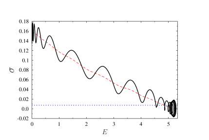
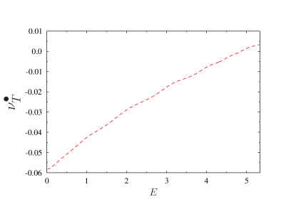
Figure 2: Results obtained for the two-dimensional cylinder wake flow at $Re=100$: (a) the growth rates $\sigma$ in reduced-order models (14)–(15) and (b) the corresponding optimal eddy viscosity $\nu_{T}^{\bullet}$ in system (16) as functions of the fluctuation energy $E$; optimal reconstructions $\sigma^{\bullet}$ and $\nu_{T}^{\bullet}$ computed by Protas et al. (2014) (red dashed lines), prediction from Galerkin model (14) (blue dotted line) and the quantity $r^{-1}\,(dr/dt)|_{r(t)}$ computed based on the solution of the Navier-Stokes problem (black solid line).

Summarizing, a negative eddy viscosity at low fluctuation values and positive at large fluctuation values can cure non-physically long transient times to the attractor. In the following we thus allow the eddy viscosity to be an essentially arbitrary function of $E$

$$\nu_{T}^{\bullet}:=\nu_{T}^{\bullet}\left(E\right).$$ (18)

In the light of the cylinder wake example, one may therefore expect small or negative values of the eddy viscosity to arise for $E<\overline{E}$ and positive values for $E>E^{a}$.

The marginal growth rates of POD models may be also related to unresolved base flow variations (Aubry et al., 1988; Podvin, 2009; Noack et al., 2003) and mode deformation during transients (Noack et al., 2003; Sapsis & Majda, 2013). While it is possible to address these issues in our framework, it would significantly complicate the exposition, hence they will not be considered in the present study.

3 Optimal eddy viscosity

In this section we describe a variational approach for determination of an optimal dependence of the nonlinear eddy viscosity $\nu_{T}$ in the Galerkin system (12) on the turbulent kinetic energy $E$. Here, “optimality” means that the eddy viscosity minimizes a performance criterion quantifying how well the evolution described by reduced-order model (12) matches the actual evolution governed by Navier-Stokes system (2). We consider a time window $[0,T]$ whose length $T$ is a parameter and assume that over this time window the flow is characterized by the resolved turbulent kinetic energy $\widetilde{E}(t)$ representing the energy content of its first $N$ POD modes, i.e.,

$$\widetilde{E}(t):=\frac{1}{2}\,\sum_{i=1}^{N}\langle\boldsymbol{u}^{\prime}(\cdot,t),\boldsymbol{u}_{i}\rangle_{L_{2}(\Omega)}^{2},$$ (19)

where $\boldsymbol{u}^{\prime}$, $\boldsymbol{u}_{i}$ and the inner product $\langle\cdot,\cdot\rangle_{L_{2}(\Omega)}$ were defined in § 2.2. This fluctuation energy is determined from the solution (here, DNS or LES) of the Navier-Stokes problem. Then, we can define the following cost functional

$${\mathcal{J}}(\nu_{T})=\frac{1}{2T}\int_{0}^{T}\left[E(t;\nu_{T})-\widetilde{E}(t)\right]^{2}\,dt,$$ (20)

where $E(t;\nu_{T})$ is the turbulent kinetic energy characterizing system (12) which depends on eddy viscosity $\nu_{T}$. Since the length $T$ of the time window on which measurements $\widetilde{E}(t)$ are available can be quite long compared to the times over which the reduced-order model (12) is capable of reproducing accurately the actual trajectory, in evaluating $E(t;\nu_{T})$ we will periodically restart system (12) using projections of the actual flow evolution on the POD modes as the initial data ${\mathbf{a}}^{0}$. More precisely, we will subdivide the interval $[0,T]$ into $M$ subintervals of length $\Delta T=T/M$, so that $[0,T]=[0,\Delta T]\cup[\Delta T,2\Delta T]\cup\ldots\cup[(M-1)\Delta T,M\Delta T]$, see figure 3. On each of the subintervals $[(m-1)\Delta T,m\Delta T]$, $m=1,\dots,M$, the Galerkin system will therefore take the form

$$\frac{da_{i}}{dt}=\sum_{j,k=0}^{N}q^{c}_{ijk}a_{j}a_{k}+\left[\nu+\nu_{T}(E(t))\right]\,\sum_{j=0}^{N}l^{\nu}_{ij}a_{j},\quad t\in((m-1)\Delta T,m\Delta T],$$ (21a)

$$a_{i}((m-1)\Delta T)=a^{0,m}_{i},\qquad i=1,\dots,N,$$ (21b)

where $a^{0,m}_{i}=\langle\boldsymbol{u}^{\prime}(\cdot,(m-1)\Delta T),\boldsymbol{u}_{i}\rangle_{L_{2}(\Omega)}$ and $m=1,\dots,M$. Periodic restarts of Galerkin system (21) ensure that its trajectory never departs too far from the projected trajectory of the actual flow, which is important given the form of the cost functional adopted in (20).

Figure 3: Schematic showing the partition of the time window $[0,T]$ into subintervals $[(m-1)\Delta T,m\Delta T]$, $m=1,\dots,M$.

The nonlinear eddy viscosity $\nu_{T}^{\circ}$ introduced in § 2.4, cf. (13), will serve as a reference and point of departure for the present optimization approach. As regards the functional form of the optimal eddy viscosity $\nu_{T}^{\bullet}$, we will make the following rather nonrestrictive assumptions (hereafter we will use the symbol $e$ as the variable corresponding to the turbulent kinetic energy $E$).

Assumption 1

1. $\nu_{T}^{\bullet}(e)$ is defined for $e\in{\mathcal{I}}:=[0,E_{\textrm{max}}]$, where $E_{\textrm{max}}$ is chosen such that $E_{\textrm{max}}>\max_{t\in[0,T]}E(t)$,

2. $\nu_{T}^{\bullet}(e)$ is a continuous function of $e$ with square-integrable derivatives on ${\mathcal{I}}$; this implies that $\nu_{T}^{\bullet}\in H^{1}({\mathcal{I}})$, where $H^{1}({\mathcal{I}})$ is the Sobolev function space equipped with the inner product (Adams & Fournier, 2005)

   $$\forall_{z_{1},z_{2}\in H^{1}({\mathcal{I}})}\qquad\big{\langle}z_{1},z_{2}\big{\rangle}_{{H^{1}({\mathcal{I}})}}=\int_{0}^{E_{\textrm{max}}}z_{1}z_{2}+\ell^{2}{\partial z_{1}\over\partial e}{\partial z_{2}\over\partial e}\,de,$$ (22)

   where $\ell>0$,

3. $$\nu_{T}^{\bullet}(0)=\nu_{T}^{\circ}(0)=0,$$ (23)

4. $$\frac{d\nu_{T}^{\bullet}}{de}\bigg{|}_{e=E_{\textrm{max}}}=\frac{d\nu_{T}^{\circ}}{de}\bigg{|}_{e=E_{\textrm{max}}}=:G.$$ (24)

Some comments are in place as regards the physical interpretation of the above assumptions. Assumption 1(a) guarantees that the optimal eddy viscosity $\nu_{T}^{\bullet}(e)$ is defined over a range of $e$ relevant for the given flow. Our experience shows that the specific value of $E_{\textrm{max}}$ does not noticeably influence the results, provided it is slightly larger than $\max_{t\in[0,T]}E(t)$, typically by a factor in the range 1.1–3.0. Assumption 1(b) concerns the minimal smoothness of the optimal eddy viscosity as a function of $e$. We emphasize that, as shown by Bukshtynov et al. (2011), omitting the differentiability requirement and assuming that $\nu_{T}^{\bullet}$ is only square-integrable ($\nu_{T}^{\bullet}\in L_{2}({\mathcal{I}})$) could in fact produce discontinuous eddy viscosities which are unphysical. Assumptions 1(c) and 1(d) imply that for limiting values of $e$ the behaviour of the optimal eddy viscosity $\nu_{T}^{\bullet}$ is the same as in the reference relation (13). More specifically, at $e=0$ the optimal eddy viscosity $\nu_{T}^{\bullet}$ will vanish, whereas at $e=E_{\textrm{max}}$ it will have the same slope (with respect to $e$) as the reference relation $\nu_{T}^{\circ}$. The latter assumption is justified by the fact, shown by Noack et al. (2011), that the reference relation (13) is accurate in the limit of large $e$. Thus, Assumption 1 ensures that for small and large values of the fluctuation energy, for which no sensitivity information can be extracted from the model, the optimal reconstruction smoothly falls back to the reference eddy viscosity (13), or any other relation chosen in its place. We add that from the practical point of view this is not a problem, because in any given flow the fluctuation energy will not exceed $\max_{t\in[0,T]}E(t)$ by a significant fraction and hence the values of $\nu_{T}^{\bullet}(e)$ for $e>\max_{t\in[0,T]}E(t)$ are not very important for the accuracy of the reduced-order model (the optimal eddy viscosity is defined for such $e$ for technical reasons only). It should be also emphasized that the optimal eddy viscosity $\nu_{T}^{\bullet}(e)$ is allowed to become negative for some values of the turbulent kinetic energy $e$.

The optimization problem for finding $\nu_{T}^{\bullet}$ can be therefore stated as follows

$$\nu_{T}^{\bullet}=\operatorname*{argmin}_{{\stackrel{{\scriptstyle\nu_{T}\in H^{1}({\mathcal{I}}),}}{{\nu_{T}(0)=0,\ \frac{d\nu_{T}}{de}\big{|}_{e=E_{\textrm{max}}}=G}}}}\ {\mathcal{J}}(\nu_{T})$$ (25)

with cost functional ${\mathcal{J}}(\nu_{T})$ given in (20) together with (21). While problem (25) is of the “parameter identification” type, it is in fact quite different from the related problems already studied in the literature on reduced-order modelling (D’Adamo et al., 2007; Artana et al., 2012; Cordier et al., 2013), in which the optimal eddy viscosity $\nu_{T}$ was sought as a function of time (i.e., an independent variable in the problem). The reduced-order model resulting from such formulation is non-autonomous and therefore restricted to the time-window and the initial condition used in the determination of the optimal eddy viscosity. Consequently, such time-dependent optimal eddy viscosity cannot be considered a proper “closure model”. On the other hand, our formulation (25) is fundamentally different and leads to an optimal eddy viscosity as a constitutive relation of the form $\nu_{T}^{\bullet}=\nu_{T}^{\bullet}((1/2)\|{\mathbf{a}}\|_{2}^{2})$, so that the corresponding reduced-order model is autonomous.

In order to ensure that optimal eddy viscosity $\nu_{T}^{\bullet}$ satisfies Assumption 1, we will adopt the “optimize-then-discretize” paradigm (Gunzburger, 2003) in solving problem (25). While solution of this problem relies on a standard gradient-based approach, it requires a specialized technique for the evaluation of gradients. Its mathematical and computational foundations were established by Bukshtynov et al. (2011) and Bukshtynov & Protas (2013), and here we use an adaptation of this approach to the identification of reduced-order models recently developed by Protas et al. (2014). Below we present the main elements of the algorithm deferring technical details to Appendix A.

The (local) minimizer $\nu_{T}^{\bullet}$ of (20) is characterized by the first-order optimality condition (Luenberger, 1969) requiring the vanishing of the Gâteaux differential ${\mathcal{J}}^{\prime}(\nu_{T};\nu^{\prime}_{T}):=\lim\limits_{\epsilon\rightarrow 0}\epsilon^{-1}\left[{\mathcal{J}}(\nu_{T}+\epsilon\nu^{\prime}_{T})-{\mathcal{J}}(\nu_{T})\right]$, i.e.,

$$\forall_{\nu^{\prime}_{T}\in H^{1}({\mathcal{I}}),\ \nu^{\prime}_{T}(0)=0,\ \frac{d\nu^{\prime}_{T}}{de}\big{|}_{e=E_{\textrm{max}}}=0}\qquad{\mathcal{J}}^{\prime}(\nu_{T}^{\bullet};\nu^{\prime}_{T})=0,$$ (26)

where $\nu^{\prime}_{T}$ is an arbitrary perturbation direction. This minimizer can be computed as $\nu_{T}^{\bullet}=\lim\limits_{n\rightarrow\infty}\nu_{T}^{(n)}$ using the following iterative procedure

$$\left\{\begin{aligned} &\nu_{T}^{(n+1)}&&=\nu_{T}^{(n)}-\tau^{(n)}\nabla{\mathcal{J}}(\nu_{T}^{(n)}),\qquad n=1,\dots,\\ &\nu_{T}^{(1)}&&=\nu_{T}^{\circ},\end{aligned}\right.$$ (27)

where the reference eddy viscosity $\nu_{T}^{\circ}$ from § 2.4 is taken as the initial guess, $n$ denotes the iteration count and $\nabla{\mathcal{J}}\;:\;{\mathcal{I}}\rightarrow{\mathbb{R}}$ is the gradient of cost functional ${\mathcal{J}}$. The length $\tau^{(n)}$ of the step along the descent direction is determined by solving line minimization problem

$$\tau^{(n)}=\operatorname*{argmin}_{\tau>0}\;{\mathcal{J}}\left(\nu_{T}^{(n)}-\tau\nabla{\mathcal{J}}_{1}(\nu_{T}^{(n)})\right)$$ (28)

which can be done efficiently using standard techniques such as Brent’s method (Press et al., 1986). For the sake of clarity, formulation (27) represents the steepest-descent method, however, in practice one typically uses more advanced minimization techniques, such as the conjugate gradient method, or one of the quasi-Newton techniques (Nocedal & Wright, 2002). Evidently, the key element of minimization algorithm (27) is the computation of the cost functional gradient $\nabla{\mathcal{J}}$. It ought to be emphasized that, while the governing system (21) is finite-dimensional, the gradient $\nabla{\mathcal{J}}$ is a function of the turbulent kinetic energy $e$ and as such represents a continuous (infinite-dimensional) sensitivity of cost functional ${\mathcal{J}}(\nu_{T})$ to the perturbations $\nu^{\prime}_{T}=\nu^{\prime}_{T}(e)$. As shown in Appendix A, the $L_{2}$ gradient of cost functional (20) can for $e\in[0,E_{\textrm{max}}]$ be evaluated as

$$\nabla^{L_{2}}{\mathcal{J}}(e)=\sum_{\stackrel{{\scriptstyle t}}{{E({\mathbf{a}}(t))=e}}}\frac{\sum_{i,j=0}^{N}l^{\nu}_{ij}a_{j}(t)a^{*}_{i}(t)}{\sum_{i=1}^{N}a_{i}(t)\left[f_{i}({\mathbf{a}}(t))+\nu_{T}((1/2)\|{\mathbf{a}}(t)\|^{2}_{2})\sum_{j=0}^{N}l_{ij}^{\nu}a_{j}(t)\right]}$$ (29)

in which $f_{i}({\mathbf{a}}(t))$ is defined in (10), whereas ${\mathbf{a}}^{*}(t)=[0,a^{*}_{1}(t),\dots,a^{*}_{N}(t)]^{T}\in{\mathbb{R}}^{N+1}$ is the solution of adjoint system

$$-\frac{da^{*}_{i}}{dt} =\sum_{j=0}^{N}A_{ji}a^{*}_{j}+\frac{a_{i}}{T}\left[E(t)-\widetilde{E}(t)\right],\quad t\in((m-1)\Delta T,m\Delta T],$$ (30a)

$$a^{*}_{i}(m\Delta T) =0,\qquad i=1,\dots,N,\quad m=1,\dots,M,$$ (30b)

where ${\bf A}$ is the linearized operator defined in Appendix A. So that it has the same dimension $(N+1)$ as the state vector ${\mathbf{a}}(t)$, cf. § 2.2, the adjoint state ${\mathbf{a}}^{*}(t)$ is defined to have an extra (zero) element in the first position. In order to ensure that the optimal eddy viscosity $\nu_{T}^{\bullet}$ possesses the smoothness and boundary behaviour required by Assumption 1, in iterations (27) we need to use the $H^{1}$ Sobolev gradient $\nabla{\mathcal{J}}=\nabla^{H^{1}}{\mathcal{J}}$ defined with respect to inner product (22), rather than the $L_{2}$ gradient given in (29). The two gradients are related through the following elliptic boundary-value problem (Protas et al., 2004)

$$\left(1-\ell^{2}\frac{d^{2}}{de^{2}}\right)\nabla^{H^{1}}{\mathcal{J}} =\nabla^{L_{2}}{\mathcal{J}} \textrm{in}\ (0,E_{\textrm{max}}),$$ (31a)

$$\nabla^{H^{1}}{\mathcal{J}} =0 \textrm{at}\ e=0,$$ (31b)

$$\frac{d}{de}\nabla^{H^{1}}{\mathcal{J}} =0 \textrm{at}\ e=E_{\textrm{max}},$$ (31c)

where $\ell\in{\mathbb{R}}$ is a parameter with the meaning of a “length scale”. Protas et al. (2004) showed that extraction of cost functional gradients in the space $H^{1}$ with the inner product defined as in (22) can be regarded as low-pass filtering the $L_{2}$ gradients with the cut-off wavenumber given by $\ell^{-1}$. As regards the behaviour of the gradients $\nabla^{H^{1}}{\mathcal{J}}$ at the endpoints of the interval ${\mathcal{I}}$, boundary conditions (31b)–(31c) ensure that all iterates $\nu_{T}^{(n)}$ have the same behaviour as the initial guess $\nu_{T}^{\circ}$, cf. Assumption 1(c,d). At every iteration (27) of the computational algorithm one first evaluates the $L_{2}$ gradient (29), which requires integration along the system trajectory in the phase space ${\mathbb{R}}^{N}$ (Protas et al., 2014), and then solves problem (31) as a “post-processing” step to obtain the Sobolev gradient $\nabla^{H^{1}}{\mathcal{J}}$. Application of this approach to identification of the optimal eddy viscosity in reduced-order models of two complex flow problems is discussed in the next section.

4 Results

In this section we present the results obtained applying the procedure from § 3 to determine the optimal eddy viscosity $\nu_{T}^{\bullet}$ for two realistic flow problems with distinct properties from the point of view of reduced-order modeling. The first one, discussed in § 4.1, concerns a 2D mixing layer at a medium Reynolds number. It features a small number of dominating frequencies and most of the flow energy is resolved by a 20-dimensional Galerkin model. The second problem, discussed in § 4.2, concerns a high Reynolds number wake flow past an Ahmed body. This flow problem is characterized by a broadband frequency spectrum such that a 100-dimensional Galerkin model resolves less than half of the total energy only.

4.1 Mixing layer model

The 2D mixing layer has a Reynolds number of $500$ based on the initial vorticity thickness $L=\delta_{v}$ and the maximum velocity of the upper stream $U=U_{1}$. The inflow is described by a $\tanh$ profile with stochastic perturbations and the velocity ratio between the upper and lower stream is equal to $U_{1}/U_{2}=3$. The observation region for the POD analysis coincides with the computational domain and is given by

$$\Omega:=\left\{(x,y)\colon 0\leq x\leq 140,\quad-28\leq y\leq 28\right\}.$$ (32)

The DNS is based on the 6th-order accurate compact finite-difference approximations for the derivatives in space and a 3rd-order accurate approximation for the derivatives with respect to time. The post-transient flow is computed over 2000 convective time units and sampled with the uniform time step $\Delta t=1$. Further details concerning the numerical approach are described by Kasten et al. (2014); Kaiser et al. (2014), and figure 4 shows a snapshot of the vorticity field in the flow. The numerical data is used to construct Galerkin system (12) with dimension $N=20$ using the procedure discussed in § 2 and setting $\kappa_{i}=1$, $i=1,\dots,N$, in (13). The dimension $N=20$ ensures that the Galerkin system captures $80\%$ of the flow energy. Optimization problem (25) is solved for a broad range of time intervals $4\leq\Delta T\leq 2000$ ($500\geq M\geq 1$) at which the governing system (21) is restarted with new initial conditions. Generally, optimal eddy viscosities with two distinct sets of properties are recovered and in order to illustrate these reconstructions below we will present the results for two representative cases with $\Delta T=10$ and $\Delta T=200$ which will be referred to as optimization over, respectively, short and long windows.

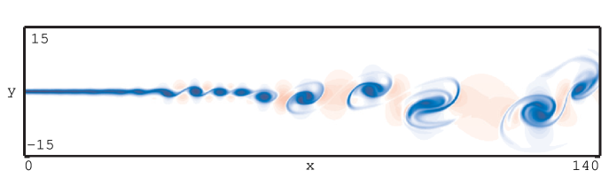
Figure 4: An instantaneous vorticity field (with red and blue representing, respectively, positive and negative values) in the 2D mixing layer flow studied in § 4.1.

We begin by presenting in figure 5 the decrease of cost functional (20) with iterations (27). We see that in the case of the short window ($\Delta T=10$) not only are the values of functional (20) smaller, but also the relative decrease achieved during iterations is less significant (about $8\%$ in figure 5a). This implies that over such short time windows the reference ansatz (13) for eddy viscosity performs satisfactorily and the improvement obtained with optimization is marginal only. On the other hand, in the case with longer time windows ($\Delta T=200$, see figure 5b), the values of the cost functional are much larger as is its relative reduction (about $74\%$) achieved with optimization. The corresponding optimal eddy viscosities $\nu_{T}^{\bullet}$ are presented in figure 6 together with the reference relation (13). We see that the optimal relation $\nu_{T}^{\bullet}$ deviates from the reference eddy viscosity $\nu_{T}^{\circ}$ for $E\in[0,100]$, which is the range of values spanned by the DNS solution, see figure 7a. On the other hand, for values of $E$ outside that range the sensitivity information is not available and therefore by construction, cf. Assumption 1(d), the optimal eddy viscosity $\nu_{T}^{\bullet}$ exhibits the same behaviour as the reference relation $\nu_{T}^{\circ}$. Two distinct behaviours are observed, with the optimal eddy viscosity $\nu_{T}^{\bullet}$ becoming negative for $E\in[0,40]$ in the case with optimization over long windows ($\Delta T=200$). We remark that this feature of the eddy viscosity was already discussed in § 2.5 where it was found to arise in a two-dimensional Galerkin model of laminar vortex shedding in the cylinder wake. The bimodal form of the optimal eddy viscosity shown in figure 6 for the short optimization window helps stabilize multiple energy levels in the flow. On the other hand, the negative eddy viscosity obtained with long optimization windows creates an excitation mechanism for the coherent structures. The physical aspects of the optimal eddy viscosities are further discussed and compared among different flow problems in § 5.

The histories of the resolved total kinetic energy $E(t)$, which is the quantity used as the performance criterion in our optimization problem, cf. (20), are presented in figure 7a, whereas in figure 7b we show the corresponding average modal energies $\overline{E}_{i}$, $i=1,\dots,20$. The mean values of the total kinetic energy $\overline{E}$ and their standard deviations are summarized in Table 1. An interesting observation one can make about this data is that the standard deviation of the turbulent kinetic energy is quite high and equal to about a third of its mean value $\overline{E}$. The reason is that the mixing-layer flow is dominated by a relatively small number of large coherent structures (cf. figure 4). Although this may not be evident from the data in Table 1, figure 7a shows that the optimal eddy viscosity $\nu_{T}^{\bullet}$ obtained with optimization over long windows ($\Delta T=200$) allows Galerkin system (12) to track the total kinetic energy $\widetilde{E}(t)$ of the original DNS simulation better than when the reference ansatz $\nu_{T}^{\circ}$ is used. This improvement is quantified by a $74\%$ decrease of the cost functional, representing the least-squares reconstruction error, cf. (20), starting from the initial guess given by the reference relation $\nu_{T}^{\circ}$ and the final iteration producing the optimal reconstruction $\nu_{T}^{\bullet}$ (figure 5b). Figure 7b indicates that this improvement is achieved with the optimal eddy viscosity $\nu_{T}^{\bullet}$ by a more accurate reconstruction of the average modal energy of the first two modes which comes at the price of a somewhat poorer reconstruction of $E_{i}$ when $i\geq 2$. On the other hand, when the optimal eddy viscosity is obtained with optimization over short windows ($\Delta T=10$), only a modest improvement is observed. The reason for that is that, as will be discussed in more detail in § 5, the optimization horizon $\Delta T=10$ is shorter than the time scale of the characteristic events in the flow. These observations are also corroborated by the results presented in figure 8, where we show the time-histories of selected Galerkin coefficients $a_{i}(t)$, $i=1,5,10,20$. In that figure we see that the optimal eddy viscosity $\nu_{T}^{\bullet}$ obtained with long optimization windows allows one to capture the amplitude $a_{1}$ of the first POD mode with a higher accuracy than when the reference relation $\nu_{T}^{\circ}$ is used. On the other hand, this optimal eddy viscosity tends to underestimate the amplitudes of the higher modes with $i=5,10,20$. Such trade-offs, which are typical of solutions obtained with optimization approaches, are a consequence of our choice of the cost functional (20) based on energy, a quantity which in the present flow is captured by the first few POD modes (figure 7b). In other words, POD modes with $i\geq 3$ contribute much less to the cost functional than the first two modes, and therefore their behaviour is to a lesser extent improved by optimization. In figure 9 we present the “unbiased” correlation function (Orfanidis, 1996)

$$C(\tau):=\frac{1}{T-\tau}\int_{\tau}^{T}\langle\boldsymbol{u}^{\prime}(\cdot,t-\tau)\cdot\boldsymbol{u}^{\prime}(\cdot,t)\rangle_{L_{2}(\Omega)}\,dt,\quad\tau\in[0,T)$$ (33)

after normalization with respect to $C(0)$. We note that using ansatz (6) and the orthogonality property of the POD modes, it can be conveniently evaluated in terms of the autocorrelations of the individual Galerkin coefficients, i.e.,

$$C(\tau)=\frac{1}{T-\tau}\sum_{i=1}^{N}\int_{\tau}^{T}a_{i}(t-\tau)a_{i}(t)\,dt.$$ (34)

In figure 9 illustrating this correlation function the oscillatory behaviour at levels around 0.3 reveals a dominant periodicity in the mixing layer. This rather low level comes from the fact that any vortex configuration is a new realization and is never exactly reproduced at any other time. The increasing correlation level as $\tau\to 2000$ indicates that the final state is close to the initial one. The large numerical values result from the narrowing of the integration window in (34) and the corresponding normalization. Due to this effect, there is hardly any averaging possible for large values of the correlation time $\tau$.

Finally, in figure 10 we compare our results concerning the history of the total kinetic energy $E(t)$ with the results obtained by Cordier et al. (2013) who used an optimization approach to determine eddy viscosities as functions of time $\nu_{T}=\nu_{T}(t)$ with different cost functionals. We see that the optimization formulation proposed here, in which the optimal eddy viscosity is sought as a function of the instantaneous turbulent kinetic energy $\nu_{T}^{\bullet}=\nu_{T}^{\bullet}(E)$, leads to a more accurate tracking of the energy $\widetilde{E}(t)$ characterizing the DNS than any of the time-dependent eddy viscosities $\nu_{T}(t)$, especially at later times ($t>800$).

Table 1: [Mixing layer] Mean resolved turbulent kinetic energy $\overline{E}$ and its standard deviation $\mathop{std}(E)$ in the different cases considered in § 4.1.

	Original DNS	System (12)	System (12) with $\nu_{T}^{\bullet}$	System (12) with $\nu_{T}^{\bullet}$
	($N=20$)	with $\nu_{T}^{\circ}$	short windows	long windows
			($\Delta T=10$)	($\Delta T=200$)
$\overline{E}$	61.73	58.43	80.84	51.27
$\mathop{std}(E)$	20.12	24.79	23.77	13.41

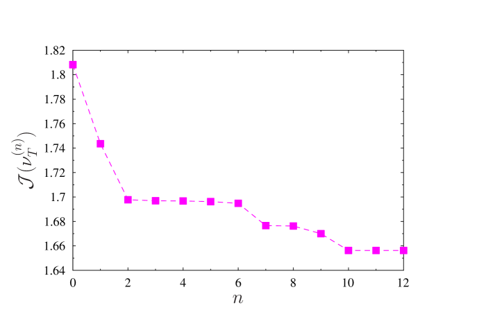
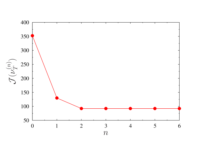
Figure 5: [Mixing layer] Decrease of the cost functional (20) with iterations $n$ for optimization over (a) over short windows ($\Delta T=10$) and (b) over long windows ($\Delta T=200$). The two sets of data are plotted on separate graphs because of the widely different values of ${\mathcal{J}}(\nu_{T}^{(n)})$.

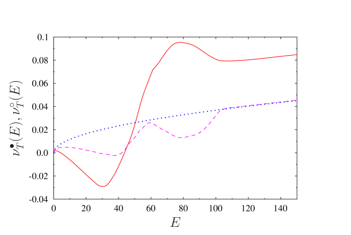
Figure 6: [Mixing layer] Optimal eddy viscosity $\nu_{T}^{\bullet}(E)$ obtained with optimization over long windows ($\Delta T=200$; red solid line) and over short windows ($\Delta T=10$; dashed purple line); reference eddy viscosity $\nu_{T}^{\circ}(E)$ is marked thick blue dotted line.

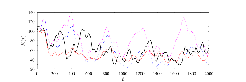
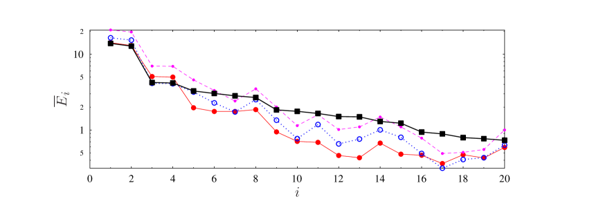
Figure 7: [Mixing layer] (a) Turbulent kinetic energy $E(t)$ as a function of time $t$ and (b) time-averaged modal energy $\overline{E}_{i}$ as a function of mode index $i$ for DNS projected on $N=20$ POD modes (thick black solid line), ROM with the reference eddy viscosity $\nu_{T}^{\circ}(E)$ (thick blue dotted line) and the optimal eddy viscosity $\nu_{T}^{\bullet}(E)$ obtained with optimization over long windows ($\Delta T=200$; red solid line) and over short windows ($\Delta T=10$; dashed purple line).

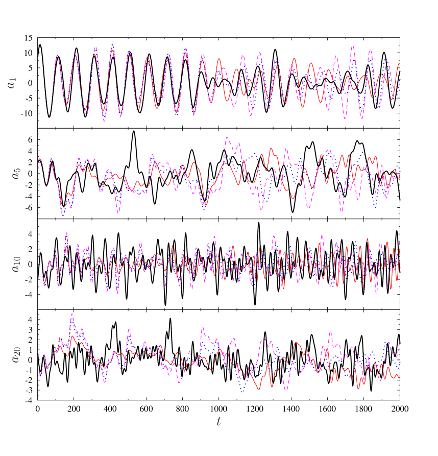
Figure 8: [Mixing layer] Galerkin expansion coefficients $a_{k}(t)$, $k=1,5,10,20$, as a function of time $t$ for DNS projected on $N=20$ POD modes (thick black solid line), ROM with the reference eddy viscosity $\nu_{T}^{\circ}(E)$ (thick blue dotted line) and the optimal eddy viscosity $\nu_{T}^{\bullet}(E)$ obtained with optimization over long windows ($\Delta T=200$; red solid line) and over short windows ($\Delta T=10$; dashed purple line).

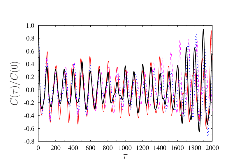
Figure 9: [Mixing layer] Normalized unbiased two-time correlation function $C(\tau)/C(0)$ for DNS projected on $N=20$ POD modes (thick black solid line), ROM with the reference eddy viscosity $\nu_{T}^{\circ}(E)$ (thick blue dotted line) and the optimal eddy viscosity $\nu_{T}^{\bullet}(E)$ obtained with optimization over long windows ($\Delta T=200$; red solid line) and over short windows ($\Delta T=10$; dashed purple line).

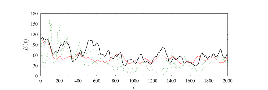
Figure 10: [Mixing layer] Comparison of turbulent kinetic energy $E(t)$ as a function of time $t$ for DNS (thick black solid line), optimal reconstruction on long windows ($\Delta T=200$; thin red solid line) and the results from Cordier et al. (2013) corresponding to three different objective functionals (dotted green lines).

4.2 Ahmed body wake model

The 3D flow over the blunt Ahmed body has the Reynolds number $Re=300,000$ based on the height $L=H$ of the body and the oncoming velocity $U=U_{\infty}$. The computational domain has dimensions $28H\times 8.05H\times 5.35H$ (length $\times$ width $\times$ height), whereas the observation domain is a small wake-centered subset of the computational domain:

$${\Omega_{0}}:=\left\{(x,y,z)\in\Omega\>\colon\>0\leq x\leq 5\,H,-0.67\,H\leq y\leq 1.12\,H,|z|\leq 1.21\,H\right\}.$$ (35)

This domain is large enough to resolve the recirculation region and the absolutely unstable wake dynamics, but at the same time small enough to keep the model dimension affordable. The LES equations are discretized in space using a hybrid of central differencing and upwind schemes applied to the convective fluxes and second-order central differences applied to the viscous and subgrid terms. The time-discretization is performed with a second-order accurate implicit method. A computational grid consisting of approximately 34 million mesh points ensures that the LES is well resolved. The post-transient flow is computed over 250 convective time units, which is half of the time window analyzed by Östh et al. (2014), and sampled with the uniform time step $\Delta t=1$. The reason for taking a shorter time window is that optimization problem (25) becomes hard to solve for very large $T$. Further details of the large eddy simulation are described by Östh et al. (2014) and a typical flow pattern is illustrated in figure 11. As expected from a flow at this Reynolds number, this flow pattern exhibits highly complex multiscale vortex structures, which makes it quite different from the mixing-layer flow illustrated in figure 4. The numerical data is used to construct Galerkin system (12) with dimension $N=100$ using the procedure discussed in § 2. In contrast to the example studied in § 4.1, in the present problem with the chosen dimension $N=100$ the Galerkin model captures only about $35\%$ of the turbulent kinetic energy of the entire flow. We emphasize that the “target” turbulent kinetic energy $\widetilde{E}(t)$ is computed based on the projection of the actual flow evolution on the first $N=100$ modes, rather than based on the entire flow field. As in the case of the mixing layer, we performed optimization calculations for a range of different $\Delta T$ and below we will show the results corresponding to two representative time intervals, namely, $\Delta T=20$ and $\Delta T=200$, which will be referred to as the short and long window, respectively.

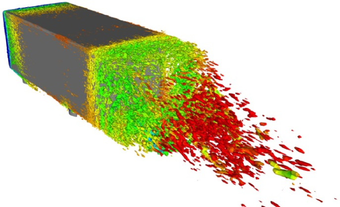
Figure 11: Illustration of a typical flow pattern in the turbulent wake behind an Ahmed body (Östh et al., 2014). The flow is visualized using the quantity $Q(\boldsymbol{x},t):=\boldsymbol{\omega}\cdot\boldsymbol{\omega}-{\bf S}:{\bf S}$ where $\boldsymbol{\omega}:=\boldsymbol{\nabla}\times\boldsymbol{u}$ is the vorticity and ${\bf S}:=(1/2)\left[\boldsymbol{\nabla}\boldsymbol{u}+(\boldsymbol{\nabla}\boldsymbol{u})^{T}\right]$ is the symmetric part of the velocity gradient tensor.

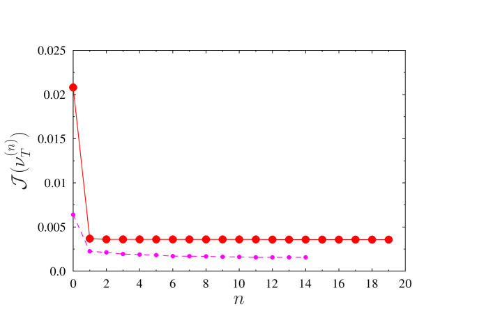
Figure 12: [Ahmed body] Decrease of the cost functional (20) with iterations $n$ for optimization over short windows ($\Delta T=20$; small purple symbols) and over long windows ($\Delta T=200$; big red symbols).

Table 2: [Ahmed body] Mean resolved turbulent kinetic energy $\overline{E}$ and its standard deviation $\mathop{std}(E)$ in the different cases considered in § 4.2.

	Original LES	System (12)	System (12) with $\nu_{T}^{\bullet}$	System (12) with $\nu_{T}^{\bullet}$
	($N=100$)	with $\nu_{T}^{\circ}$	short windows	long windows
			($\Delta T=20$)	($\Delta T=200$)
$\overline{E}$	0.2739	0.4514	0.3315	0.2759
$\mathop{std}(E)$	0.0820	0.0562	0.0504	0.0570

Decrease of cost functional (20) with iterations is shown in figure 12 in which a significant reduction can be observed in both cases. This implies that the reference eddy viscosity (13) can be improved by performing optimization on either short or long time intervals. The values of the cost functional corresponding to long optimization intervals are again larger which is due to the fact that, with fewer restarts, the trajectory of (21) diverges further away from the projected trajectory of the actual flow. The resulting optimal eddy viscosities $\nu_{T}^{\bullet}$ are presented in figure 13, together with the reference relation (13). We see that the obtained profile of the optimal eddy viscosity has a similar general form for both values of $\Delta T$, except that it is smoother for the case of the longer window. This suggests that allowing for a longer assimilation interval before the constraint system (21) is restarted with a new initial condition may have a regularizing effect (i.e., may produce smoother optimal eddy viscosity relations). We also note that, in contrast to the findings of § 4.1, in the present case the optimal eddy viscosity $\nu_{T}^{\bullet}$ is uniformly increased with respect to the reference relation $\nu_{T}^{\circ}$. While the function $\nu_{T}^{\bullet}(E)$ is defined for $E\in[0,2]$, cf. Assumption 1(a), deviations from the reference relation $\nu_{T}^{\circ}(E)$ are confined to the range $[0,0.7]$ which is approximately the range of energy values visited by the system trajectory, (more precisely, $\max_{t\in[0,T]}E(t)\approx 0.6$ as can be seen from figure 14a). Outside that range the sensitivity information is not available and the optimal eddy viscosity $\nu_{T}^{\bullet}$ essentially coincides with the reference relation $\nu_{T}^{\circ}$, cf. Assumption 1(d). Discussion of the physical aspects of the optimal eddy viscosities obtained for the Ahmed body wake is deferred to § 5. Figure 14a shows the improvement in the tracking of the instantaneous turbulent kinetic energy $\widetilde{E}(t)$ achieved by Galerkin system (12) with the optimal eddy viscosity $\nu_{T}^{\bullet}$ with respect to the use of the reference relation $\nu_{T}^{\circ}$. We see that the optimal eddy viscosities $\nu_{T}^{\bullet}$ obtained both with short and long optimization windows allow the Galerkin model to track the target energy $\widetilde{E}(t)$ more accurately than with the reference relation, although in fairness to the latter it has to be recognized that the choice of $\nu_{T}^{a}$ in (13) was not optimal resulting in overestimated turbulent kinetic energy. In fact, the present approach may be considered a systematic way of using data to refine closures proposed based on theoretical or empirical arguments. The above observations are confirmed by the values of the mean turbulent kinetic energy and its standard deviation collected for the different cases in Table 2. We note, in particular, that with optimization performed over long time windows the proposed approach captures the mean energy of the flow with the accuracy of two significant digits. The average modal energies $\overline{E}_{i}$, $i=1,\dots,100$, are presented in figure 14b and we see that the optimal eddy viscosity $\nu_{T}^{\bullet}$ yields an improved reconstruction essentially across the entire mode spectrum. This should be contrasted with figure 7b, where an improvement was observed only for the first energy-containing modes. This difference is attributed to the spectral properties of the two flows and our choice of the cost functional (20) — while in the mixing-layer flow most of the flow energy is contained in the first few modes, in the Ahmed body wake this energy is spread over a very large number of modes. These findings are corroborated by the plots of the time-histories of selected Galerkin coefficients $a_{i}(t)$, $i=1,5,25,100$, shown in figure 15. In those plots we note that, unlike the case of the mixing layer, some improvement is also obtained for higher modes. Finally, the correlation functions (33)–(34) for the POD projections of the original flow data and the solutions of the reduced-order model (12) with the reference and optimal eddy viscosities are shown in figure 16. All curves reveal a small oscillatory component corresponding to the von Kármán vortex shedding at the Strouhal number $St_{H}\approx 0.2$. These oscillations are not very pronounced in the velocity fields, but show up more clearly in the pressure field and the aerodynamic forces as reported by Östh et al. (2014). The curve corresponding to the LES data shows an anti-correlation after roughly 100 convection times. This behaviour can be traced back to the asymmetric base flow drift from a state with positive to a state with negative transverse forces. This base flow drift is resolved by the shift mode ($a_{1}$ in Figure 15). From the same plot of the POD mode coefficients, the reduced-order models are seen to display a smaller base flow variation than exhibited by the actual LES data. This explains the decreased variation of the correlation function of the POD models. We emphasize that it is very difficult for POD models to resolve multi-scale phenomena, such as vortex shedding combined with base flow drifts, the time-scales of which are two orders of magnitude apart. For further details concerning the reduced-order modelling of the Ahmed body wake, we refer the reader to the original publication by Östh et al. (2014).

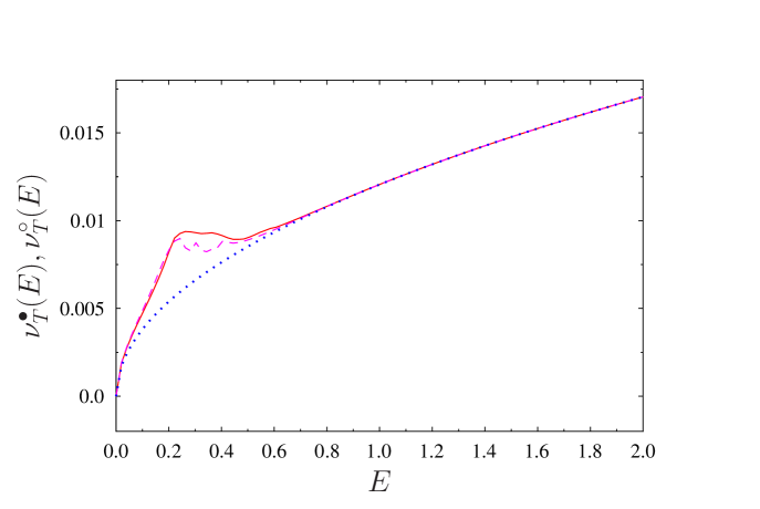
Figure 13: [Ahmed body] Optimal eddy viscosity $\nu_{T}^{\bullet}(E)$ obtained with optimization over long windows ($\Delta T=200$; red solid line) and over short windows ($\Delta T=20$; dashed purple line); reference eddy viscosity $\nu_{T}^{\circ}(E)$ is marked thick blue dotted line.

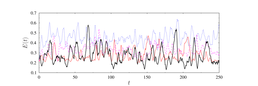
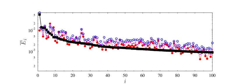
Figure 14: [Ahmed body] (a) Turbulent kinetic energy $E(t)$ as a function of time $t$ and (b) time-averaged modal energy $\overline{E}_{i}$ as a function of mode index $i$ for LES projected on $N=100$ POD modes (thick black solid line), ROM with the reference eddy viscosity $\nu_{T}^{\circ}(E)$ (thick blue dotted line) and the optimal eddy viscosity $\nu_{T}^{\bullet}(E)$ obtained with optimization over long windows ($\Delta T=200$; red solid line) and over short windows ($\Delta T=20$; dashed purple line).

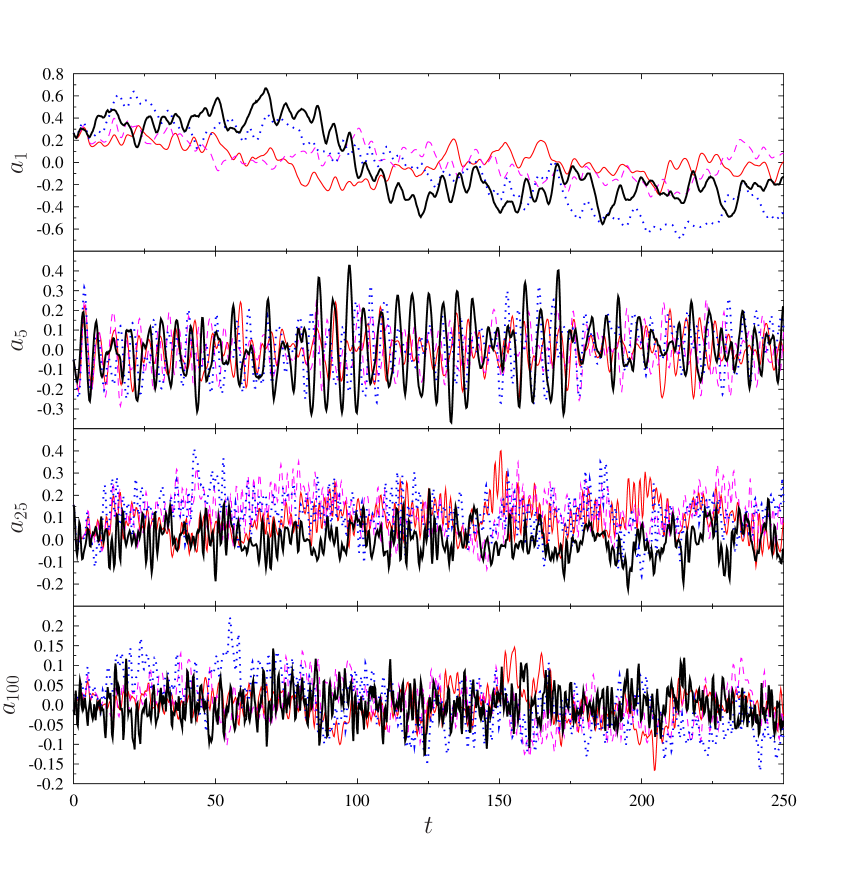
Figure 15: [Ahmed body] Galerkin expansion coefficients $a_{k}(t)$, $k=1,5,25,100$, as a function of time $t$ for LES projected on $N=100$ POD modes (thick black solid line), ROM with the reference eddy viscosity $\nu_{T}^{\circ}(E)$ (thick blue dotted line) and the optimal eddy viscosity $\nu_{T}^{\bullet}(E)$ obtained with optimization over long windows ($\Delta T=200$; red solid line) and over short windows ($\Delta T=20$; dashed purple line).

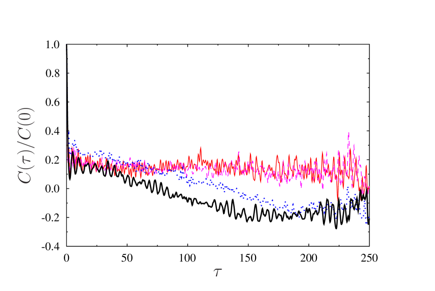
Figure 16: [Ahmed body] Normalized unbiased two-time correlation function $C(\tau)/C(0)$ for LES projected on $N=100$ POD modes (thick black solid line), ROM with the reference eddy viscosity $\nu_{T}^{\circ}(E)$ (thick blue dotted line) and the optimal eddy viscosity $\nu_{T}^{\bullet}(E)$ obtained with optimization over long windows ($\Delta T=200$; red solid line) and over short windows ($\Delta T=20$; dashed purple line).

5 Conclusions and future directions

We have proposed an optimal nonlinear eddy viscosity relation for a large class of reduced-order models which improves on the results from a number of earlier studies. In the pioneering investigation concerning POD-based reduced-order models by Aubry et al. (1988), a single constant eddy viscosity parameter was assumed. Rempfer & Fasel (1994b) proposed a mode-dependent refinement of the constant eddy viscosity ansatz which significantly improves the accuracy of reduced-order models. Later, Noack et al. (2011) derived a nonlinear eddy viscosity as a function of the square root of the resolved fluctuation energy in which constant ratios between the modal energies were assumed. This nonlinearity guarantees the boundedness of the Galerkin solution (Cordier et al., 2013). As shown by Östh et al. (2014), combinations of modal and nonlinear eddy viscosities may improve the accuracy and robustness of POD-based reduced-order models. The key new aspect of the approach proposed here is that the eddy viscosity relations are defined to be optimal in a mathematically precise sense. As such, these relations can be viewed as systematic, data-based refinements of closures obtained from theoretical or empirical considerations.

The current study addresses the limitations of earlier approaches by considering the eddy viscosity as an arbitrary function of the resolved turbulent kinetic energy which is optimized by matching the fluctuation level of the reduced-order model to the corresponding quantity of the reference data. This optimization is performed with a generalization of the 4D-VAR data assimilation method adopted for the reconstruction of constitutive equations by Bukshtynov et al. (2011); Bukshtynov & Protas (2013).

POD models with the optimal eddy viscosity are constructed for three shear flows with progressively richer dynamics spanning the laminar and turbulent regimes. First, the two-dimensional POD model for the transient behaviour in the 2D cylinder wake is recalled from an earlier study (Protas et al., 2014). Here, a negative eddy viscosity is derived at low fluctuation levels to compensate for the significantly underpredicted growth rate of the POD model (figure 2b). On the other hand, on the limit cycle and beyond, a positive eddy viscosity models the energy transfer to the higher-order modes. In this example, the eddy viscosity not only assures correct amplitudes on the limit cycle, but also yields more accurate transient times (figure 2a).

Second, a 20-dimensional POD model of the 2D mixing layer at $Re=500$ with velocity ratio $3$ is investigated. The starting point was a reduced-order model with a single nonlinear eddy viscosity calibrated against a DNS of the Navier-Stokes system by Cordier et al. (2013). Good agreement between the POD model and the DNS was observed with respect to the frequency content and the modal fluctuation levels for the energy-containing modes (figures 7b and 8). Surprisingly, the optimal eddy viscosity significantly deviates from the square-root ansatz (13) and attains negative values for a range of low fluctuation levels, thus accelerating the slow transients of the reduced-order model (Noack et al., 2005). However, the optimal eddy viscosity $\nu_{T}^{\bullet}$ is larger than the square-root ansatz $\nu_{T}^{\circ}$ at larger fluctuation levels thus limiting more energetic events (figure 6).

Third, a 100-dimensional POD model of the 3D Ahmed body wake at Reynolds number $300,000$ is constructed. The starting point is a large eddy simulation and the best one from the Galerkin POD models developed and analyzed by Östh et al. (2014, model “GS-D”) is used as a benchmark. The sub-scale turbulence representation in this model includes the modal eddy viscosities proportional to the square-root of the resolved turbulent kinetic energy (cf. § 2.4). The optimal eddy viscosity respects the ratio between the modal viscosities while allowing for an arbitrary scaling with the resolved turbulent kinetic energy. As regards the comparison between the optimal and reference eddy viscosity (figure 13), for all values of the fluctuation energy the optimal eddy viscosity $\nu_{T}^{\bullet}$ exhibits larger values than the reference relation $\nu_{T}^{\circ}$, consistently with the overprediction of the energy fluctuation level in the latter case (figure 14a).

A key advantage of variational optimization formulations such as the one proposed here is that they reveal certain performance trade-offs inherent in the solution of complex flow problems which can hardly be identified based on the physical intuition alone. This is evident when one compares the results obtained in the mixing-layer flow, which can be considered “laminar”, and the Ahmed body wake, which is “turbulent” in all respects. Since in the first case most of the turbulent kinetic energy was associated with the first two POD modes, these were also the components of the ROM mostly affected by the optimization process (figure 7b). On the other hand, in the second case, in which the energy was distributed more evenly among different modes, optimization affected the entire spectrum (cf. figure 14b). This comparison demonstrates that the optimal eddy viscosities do indeed adapt to situations characterized by essentially different flow physics. At the same time, these results also reveal certain fundamental performance limitations inherent in the ansatz $\nu_{T}=\nu_{T}(E)$ commonly used for the eddy viscosity. Needless to say, this process can be modified by using a different cost functional and/or a different ansatz for $\nu_{T}$. For example, adopting a cost functional penalizing deviations of, say, enstrophy rather than energy, would have certainly yielded different results. We emphasize that such decisions are a part of the problem formulation and can be handled by the proposed solution approach in a straightforward manner.

The observed features of the optimal eddy viscosity identified as a function of the fluctuation energy deserve additional discussion. From the results we conjecture that the optimal eddy viscosity $\nu_{T}^{\bullet}$ does not strongly depend on the chosen time window $[0,T]$, provided that it is equal to or longer than the characteristic time scale of the dominant coherent structures. This was the case for both of the time windows used for the Ahmed body wake (figure 14a), but not for the short time window used for the mixing layer (figure 7a). Secondly, the eddy viscosity obtained for the mixing layer shows two minima helping stabilize two different energy levels (figure 6). This bimodal behaviour is consistent with the cluster-based analysis of the same data performed by Kaiser et al. (2014). It is shown there that the mixing layer flow has two quasi-attractors: one which is dominated by the Kelvin-Helmholtz instability at a lower energy level and another one dominated by period-doubling at a higher energy level. Thirdly, the mixing layer model exhibits a negative eddy viscosity while the model of the Ahmed body flow does not. We conjecture that this difference has two reasons: the first is that the fluctuation levels of the mixing layer have relatively larger variations (figure 7a), hence we can estimate transient times for this 2D flow better than for the 3D wake; the second is that a negative eddy viscosity excites coherent structures with similar scales in the POD model of the mixing layer flow. On the other hand, for the Ahmed body wake, a negative eddy viscosity would imply that the strongly damped high-order modes would suddenly become excited which would in turn lead to an unphysical inverse energy cascade. Summarizing, the different features of the optimal eddy viscosity found for the 2D and 3D shear flows are consistent with our expectations based on the behaviour of POD models.

Concerning the choice of the parameters in the optimization formulation, we note that the cost functional tracking the error of the fluctuation energy gives quite comparable results over different time windows (cf. figure 3), provided that the windows cover at minimum several characteristic flow periods. This was the case for the Ahmed body flow in which the shedding period was 5-10 time units, whereas optimization was performed over intervals with $\Delta T=20$ and $\Delta T=200$ (figure 14a). On the other hand, for the mixing layer the shorter window with $\Delta T=10$ covered only about half of the Kelvin-Helmholtz shedding period (figure 7a) and the resulting optimal eddy viscosity was significantly different from the relations found by solving optimization problem (25) with subintervals 10 times longer (figure 6). As regards Assumption 1 and its validity, we remark that statements (a) and (b) are mathematical in nature and ensure that model (12) is well-posed. Statements (c) and (d) stipulate that for values of $E$ for which the sensitivity information is not available the optimal eddy viscosity $\nu_{T}^{\bullet}(E)$ should revert to some chosen reference relation, in our case relation (13).

In providing a closure relation for unresolved fluctuations based on solution data, the proposed approach to identifying the optimal eddy viscosity bears some resemblance to the “optimal LES” methodology which originated with Langford & Moser (1999). However, it differs from the optimal LES in that our optimal eddy viscosity $\nu_{T}^{\bullet}$ is reconstructed in a non-parametric manner. The proposed closure strategy can be employed in a straightforward manner to identify closure relations depending on one variable for a large class of reduced-order models both for laminar and turbulent flows. A highly relevant problem complementary to the problem solved in this study is optimization of the dependence of the eddy viscosity on the mode index $i$ while keeping the dependence on the turbulent kinetic energy fixed. The approach developed here can be adapted to solve such problems by treating the discrete mode index $i$ as a continuous variable, i.e., an effective wavenumber of the mode. It will be interesting to see whether such a formulation can lead to improved performance with respect to the ansatz $\nu_{T}=\nu_{T}(E)$ used in the present investigation. This problem will be studied in the near future. Another related problem concerns determination of optimal turbulence closure strategies for simplified flow models defined in the PDE setting such as the RANS and LES approaches (in fact, these are the type of problems the reconstruction method we used was initially developed for, see Bukshtynov et al. (2011); Bukshtynov & Protas (2013)). As regards LES models, an interesting open problem is determination of optimal wall damping functions (Driest, 1956). Problems of such type also arise in fundamental turbulence research, for example, in the context of the Kármán-Howarth equation. Other, possibly less obvious, extensions of this methodology include optimal identification of inertial manifolds and feedback control laws, and the authors are already pursuing these applications in the context of closed-loop turbulence control.

Appendix A Derivation of Gradient Expression

In this appendix we derive expression (29) for the $L_{2}$ gradient of cost functional (20). The key observation is that, since the Gâteaux differential of ${\mathcal{J}}(\nu_{T})$ appearing in (26) is a bounded linear functional with respect to its second argument $\nu_{T}^{\prime}\in{\mathcal{X}}({\mathcal{I}})$, ${\mathcal{X}}({\mathcal{I}})$ being an appropriate Hilbert function space, by the Riesz representation theorem (Berger, 1977) we have

$$\forall_{\nu_{T}^{\prime}\in{\mathcal{X}}({\mathcal{I}})}\quad{\mathcal{J}}^{\prime}(\nu_{T};\nu_{T}^{\prime})=\Big{\langle}\nabla^{{\mathcal{X}}}{\mathcal{J}},\nu_{T}^{\prime}\Big{\rangle}_{{\mathcal{X}}({\mathcal{I}})},$$ (36)

where $\langle\cdot,\cdot\rangle_{{\mathcal{X}}({\mathcal{I}})}$ denotes the inner product in the space ${\mathcal{X}}({\mathcal{I}})$. We identify the Riesz representer $\nabla^{{\mathcal{X}}}{\mathcal{J}}$ as the gradient of ${\mathcal{J}}$ with respect to the topology of the space ${\mathcal{X}}({\mathcal{I}})$ (in the present problem, we have either ${\mathcal{X}}({\mathcal{I}})=L_{2}({\mathcal{I}})$ or ${\mathcal{X}}({\mathcal{I}})=H^{1}({\mathcal{I}})$). We begin by computing the Gâteaux differential of (20) which yields

$${\mathcal{J}}^{\prime}(\nu_{T};\nu_{T}^{\prime})=\frac{1}{T}\int_{0}^{T}\left[E(t)-\widetilde{E}(t)\right]E^{\prime}(t)\,dt=\frac{1}{T}\int_{0}^{T}\left[E(t)-\widetilde{E}(t)\right]\sum_{i=1}^{N}a_{i}(t)a^{\prime}_{i}(t)\,dt,$$ (37)

where $E^{\prime}:=\sum_{i=1}^{N}a_{i}a^{\prime}_{i}$ and $a^{\prime}_{i}(t)$, $i=1,\dots,N$, solve the linearization of system (21). Following the approach described by Protas et al. (2014), this linearization can be shown to have the form

$$\frac{da^{\prime}_{i}}{dt}=\sum_{j=0}^{N}\left[\sum_{k=0}^{N}(q_{ijk}+q_{ikj})a_{k}+l^{\nu}_{ij}\left(\nu+\nu_{T}(E(t))+\frac{d\nu_{T}}{de}a_{i}a_{j}\right)\right]a^{\prime}_{j}+\nu^{\prime}_{T}(E(t))\,\sum_{j=0}^{N}l^{\nu}_{ij}a_{j},$$

$$\phantom{\frac{da^{\prime}_{i}}{dt}}=:\sum_{j=0}^{N}A_{ij}a^{\prime}_{j}+\nu^{\prime}_{T}(E(t))\,\sum_{j=0}^{N}l^{\nu}_{ij}a_{j},\qquad t\in((m-1)\Delta T,m\Delta T],$$ (38a)

$$a^{\prime}_{0}(t)=0,$$ (38b)

$$a^{\prime}_{i}((m-1)\Delta T)=0,\qquad i=1,\dots,N,\quad m=1,\dots,M,$$ (38c)

where the second line in (38a) defines the linear operator ${\bf A}$. We note that differential (37) is not yet in a form consistent with Riesz representation (36), because the perturbation variable $\nu^{\prime}_{T}$ does not enter as a linear factor in (37), but is instead hidden in a source term in equation (38a). In order to transform (37) into Riesz form (36), we introduce the adjoint state ${\mathbf{a}}^{*}(t)=[0,a^{*}_{1}(t),\dots,a^{*}_{N}(t)]^{T}\in{\mathbb{R}}^{N+1}$, so that integrating it against the perturbation equation (38a) and applying integration by parts we obtain

$$\sum_{i=1}^{N}\,\int_{0}^{T}\left(\frac{da^{\prime}_{i}}{dt}-\sum_{j=0}^{N}A_{ij}a^{\prime}_{j}-\nu^{\prime}_{T}(E(t))\,\sum_{j=0}^{N}l^{\nu}_{ij}a_{j}\right)a^{*}_{i}\,dt=$$ (39)

$$\sum_{i=1}^{N}a^{\prime}_{i}a^{*}_{i}\big{|}_{t=0}^{t=T}+ \sum_{i=1}^{N}\,\int_{0}^{T}a^{\prime}_{i}\left(-\frac{da^{*}_{i}}{dt}-\sum_{j=0}^{N}A_{ji}a^{*}_{j}\right)\,dt-\int_{0}^{T}\nu^{\prime}_{T}(E(t))\,\sum_{i=1,j=0}^{N}l^{\nu}_{ij}a_{j}a^{*}_{i}\,dt=0.$$

Since $a_{0}^{*}(t)\equiv 0$, summation over index $i$ in (39) starts at 1. Defining the adjoint system as in (30), and using it together with (37) and (38), we obtain from (39)

$${\mathcal{J}}^{\prime}(\nu_{T};\nu_{T}^{\prime})=\int_{0}^{T}\nu^{\prime}_{T}(E(t))\,\sum_{i,j=0}^{N}l^{\nu}_{ij}a_{j}a^{*}_{i}\,dt.$$ (40)

In order to transform this expression to the Riesz form induced by ${\mathcal{X}}(I)=L_{2}({\mathcal{I}})$, i.e.,

$${\mathcal{J}}^{\prime}(\nu_{T};\nu_{T}^{\prime})=\int_{0}^{E_{\textrm{max}}}\nabla^{L_{2}}{\mathcal{J}}\,\nu_{T}^{\prime}\,de,$$ (41)

we need to change the integration variable in (40) from time $t$ to turbulent kinetic energy $e$

$$\frac{de}{dt}=\sum_{i=1}^{N}a_{i}\frac{da_{i}}{dt}=\sum_{i=1}^{N}a_{i}\left(f_{i}({\mathbf{a}})+\nu_{T}(E(t))\,\sum_{j=0}^{N}l^{\nu}_{ij}a_{j}\right)$$ (42)

$$\Longrightarrow\quad dt=\frac{de}{\sum_{i=1}^{N}a_{i}\left[f_{i}({\mathbf{a}})+\nu_{T}(E(t))\,\sum_{j=0}^{N}l^{\nu}_{ij}a_{j}\right]},$$

so that Gâteaux differential (40) becomes

$${\mathcal{J}}^{\prime}(\nu_{T};\nu_{T}^{\prime}) =\int_{{\mathcal{C}}}\frac{\sum_{i,j=0}^{N}l^{\nu}_{ij}a_{j}a^{*}_{i}}{\sum_{i=1}^{N}a_{i}\left[f_{i}({\mathbf{a}})+\nu_{T}(E(t))\,\sum_{j=0}^{N}l^{\nu}_{ij}a_{j}\right]}\,\nu^{\prime}_{T}(e)\,de$$

$$=\int_{0}^{E_{\textrm{max}}}\sum_{\stackrel{{\scriptstyle t}}{{E({\mathbf{a}}(t))=e}}}\frac{\sum_{i,j=0}^{N}l^{\nu}_{ij}a_{j}a^{*}_{i}}{\sum_{i=1}^{N}\big{|}a_{i}f_{i}({\mathbf{a}})+\nu_{T}(E(t))\,\sum_{j=0}^{N}l^{\nu}_{ij}a_{i}a_{j}\big{|}}\,\nu^{\prime}_{T}(e)\,de,$$ (43)

where the first expression on the right-hand side in (43) is an integral over the system trajectory ${\mathcal{C}}$ in the phase space ${\mathbb{R}}^{n}$ (i.e., a line integral in which $de$ can be either positive or negative), whereas the second expression is a definite integral consistent with Riesz form (41). Thus, identifying (43) with (41), we finally obtain gradient expression (29).

References

- Adams & Fournier (2005) Adams, R. A. & Fournier, J. F. 2005 Sobolev Spaces. Elsevier.
- Artana et al. (2012) Artana, G., Cammilleri, A., Carlier, J. & Mémin, E. 2012 Strong and weak constraint variational assimilations for reduced-order fluid flow modeling. J. Comp. Phys. 231, 3264–3288.
- Aubry et al. (1988) Aubry, N. Holmes, P. Lumley, J. L. & Stone, E. 1988 The dynamics of coherent structures in the wall region of a turbulent boundary layer. J. Fluid Mech. 192, 115–173.
- Balajewicz et al. (2013) Balajewicz, M., Dowell, E. H. & Noack, B. R. 2013 Low-dimensional modelling of high-Reynolds-number shear flows incorporating constraints from the Navier-Stokes equation. J. Fluid Mech. 729, 285–308.
- Berger (1977) Berger, M. S. 1977 Nonlinearity and Functional Analysis. Academic Press.
- Bukshtynov & Protas (2013) Bukshtynov, V. & Protas, B. 2013 Optimal reconstruction of material properties in complex multiphysics phenomena. J. Comp. Phys. 242, 889–914.
- Bukshtynov et al. (2011) Bukshtynov, V., Volkov, O. & Protas, B. 2011 On optimal reconstruction of constitutive relations. Physica D 240, 1228–1244.
- Cacuci et al. (2013) Cacuci, D. G. Navon, I. M. & Ionescu-Bujor, M. 2013 Computational Methods for Data Evaluation and Assimilation. Oxford, UK: Chapman & Hall.
- Cordier et al. (2013) Cordier, L. Noack, B. R. Daviller, G. Delvile, J. Lehnasch, G. Tissot, G. Balajewicz, M. & Niven, R.K. 2013 Control-oriented model identification strategy. Exp. Fluids 54, Article 1580.
- D’Adamo et al. (2007) D’Adamo, J., Papadakis, N., Mémin, E. & Artana, G. 2007 Variational assimilation of POD low-order dynamical systems. J. Turb. 9, 1–22.
- Deane et al. (1991) Deane, A. E. Kevrekidis, I. G. Karniadakis, G. E. & Orszag, S. A. 1991 Low-dimensional models for complex geometry flows: Application to grooved channels and circular cylinders. Phys. Fluids A 3, 2337–2354.
- Driest (1956) Driest, E.R. Van 1956 On turbulent flow near a wall. J. Aero. Sci. 23, 1007.
- Fletcher (1984) Fletcher, C. A. J. 1984 Computational Galerkin Methods, 1st edn. New York: Springer.
- Galletti et al. (2004) Galletti, G. Bruneau, C. H. Zannetti, L. & Iollo, A. 2004 Low-order modelling of laminar flow regimes past a confined square cylinder. J. Fluid Mech. 503, 161–170.
- Gunzburger (2003) Gunzburger, M. D. 2003 Perspectives in Flow Control and Optimization. SIAM.
- Hemati et al. (2014) Hemati, M. S., Eldredge, J. D. & Speyer, J. L. 2014 Improving vortex models via optimal control theory. J. Fluids Struct. (in print).
- Holmes et al. (2012) Holmes, P. Lumley, J. L. Berkooz, G. & Rowley, C. W. 2012 Turbulence, Coherent Structures, Dynamical Systems and Symmetry, 2nd edn. Cambridge: Cambridge University Press.
- Kaiser et al. (2014) Kaiser, E. Noack, B. R. Cordier, L. Spohn, A. Segond, M. Abel, M. W. Daviller, G. Östh, J. Krajnović, S. & Niven, R. K. 2014 Cluster-based reduced-order modelling of a mixing layer. J. Fluid Mech. (in print).
- Kalnay (2003) Kalnay, E. 2003 Atmospheric Modeling, Data Assimilation and Predictability. Cambridge University Press.
- Kasten et al. (2014) Kasten, J. Reininghaus, J. Hotz, I. Hege, H.-C. Noack, B. R. Daviller, G. Comte, P. & Morzyński, M. 2014 Acceleration feature points of unsteady shear flows. Tech. Rep. 1401.2462 [physics.fui-dyn]. arXiv.
- Kutz (2013) Kutz, J. N. 2013 Data-Driven Modeling & Scientific Computation: Methods for Complex Systems & Big Data. Oxford University Press.
- Lamb (1945) Lamb, Sir H. 1945 Hydrodynamics, 6th edn. New York: Dover Publications.
- Langford & Moser (1999) Langford, J. A. & Moser, R. D. 1999 Optimal LES formulations for isotropic turbulence. Journal of Fluid Mechanics 398, 321–346.
- Liberzon et al. (2007) Liberzon, A., Lüthi, B., Guala, M., Kinzelbach, W. & Tsinober, A. 2007 On anisotropy of turbulent flows in regions of ”negative eddy viscosity”. In Progress in Turbulence II, Proceedings of the iTi Conference in Turbulence 2005 (ed. M. Oberlack, G. Khujadze, S. Günther and T. Weller, M. Frewer, J. Peinke & S. Barth), Springer Proceedings in Physics, vol. 109. Springer.
- Luenberger (1969) Luenberger, D. 1969 Optimization by Vector Space Methods. John Wiley and Sons.
- Lumley (1970) Lumley, J.L. 1970 Stochastic Tools in Turbulence. New York: Academic Press.
- Ma & Karniadakis (2002) Ma, X. & Karniadakis, G. E. 2002 A low-dimensional model for simulating three-dimensional cylinder flow. J. Fluid Mech. 458, 181–190.
- Noack et al. (2003) Noack, B. R. Afanasiev, K. Morzyński, M. Tadmor, G. & Thiele, F. 2003 A hierarchy of low-dimensional models for the transient and post-transient cylinder wake. J. Fluid Mech. 497, 335–363.
- Noack et al. (2011) Noack, B. R. Morzyński, M. & Tadmor, G. 2011 Reduced-Order Modelling for Flow Control. CISM Courses and Lectures 528. Vienna: Springer-Verlag.
- Noack et al. (2005) Noack, B. R. Papas, P. & Monkewitz, P. A. 2005 The need for a pressure-term representation in empirical Galerkin models of incompressible shear flows. J. Fluid Mech. 523, 339–365.
- Nocedal & Wright (2002) Nocedal, J. & Wright, S. 2002 Numerical Optimization. Springer.
- Orfanidis (1996) Orfanidis, S. J. 1996 Optimum Signal Processing. An Introduction., 2nd edn. Prentice-Hall.
- Östh et al. (2014) Östh, J., Noack, B. R., Krajnović, S., Barros, D. & Borée, J. 2014 On the need for a nonlinear subscale turbulence term in pod models as exemplified for a high reynolds number flow over an ahmed body. J. Fluid Mech. 747, 518–544.
- Podvin (2009) Podvin, B. 2009 A proper-orthogonal-decomposition based model for the wall layer of a turbulent channel flow. Phys. Fluids 21, 015111–118.
- Press et al. (1986) Press, W. H., Flanner, B. P., Teukolsky, S. A. & Vetterling, W. T. 1986 Numerical Recipes: the Art of Scientific Computations. Cambridge University Press.
- Protas et al. (2004) Protas, B., Bewley, T. & Hagen, G. 2004 A comprehensive framework for the regularization of adjoint analysis in multiscale pde systems. J. Comp. Phys. 195, 49–89.
- Protas et al. (2014) Protas, B., Noack, B. R. & Morzynski, M. 2014 An optimal model identification for oscillatory dynamics with a stable limit cycle. J. Nonlin. Sci. 24, 245–275.
- Rempfer & Fasel (1994a) Rempfer, D. & Fasel, F.H. 1994a Evolution of three-dimensional coherent structures in a flat-plate boundary-layer. J. Fluid Mech. 260, 351–375.
- Rempfer & Fasel (1994b) Rempfer, D. & Fasel, F. H. 1994b Dynamics of three-dimensional coherent structures in a flat-plate boundary-layer. J. Fluid Mech. 275, 257–283.
- Sapsis & Majda (2013) Sapsis, T. P. & Majda, A.J. 2013 Statistically accurate low-order models for uncertainty quantification in turbulent dynamical systems. Proc. Natl. Acad. Sci USA 110, 13705–13710.
- Sirovich (1987) Sirovich, L. 1987 Turbulence and the dynamics of coherent structures, Part I: Coherent structures. Quart. Appl. Math. XLV, 561–571.
- Wang et al. (2011) Wang, Z. Akhtar, I. Borggaard, J. & Iliescu, T. 2011 Two-level discretizations of nonlinear closure models for proper orthogonal decomposition. J. Comp. Phys. 230, 126–146.
- Wang et al. (2012) Wang, Z., Akhtar, I., Borggaard, J. & Iliescu, T. 2012 Proper orthogonal decomposition closure models for turbulent flows: A numerical comparison. Comput. Methods Appl. Mech. Engrg. 237-240, 10–26.