Moving and merging of Dirac points on a square lattice and hidden symmetry protection

Abstract

First, we study a square fermionic lattice that supports the existence of massless Dirac fermions, where the Dirac points are protected by a hidden symmetry. We also consider two modified models with a staggered potential and the diagonal hopping terms, respectively. In the modified model with a staggered potential, the Dirac points exist in some range of magnitude of the staggered potential, and move with the variation of the staggered potential. When the magnitude of the staggered potential reaches a critical value, the two Dirac points merge. In the modified model with the diagonal hopping terms, the Dirac points always exist and just move with the variation of amplitude of the diagonal hopping. We develop a mapping method to find hidden symmetries evolving with the parameters. In the two modified models, the Dirac points are protected by this kind of hidden symmetry, and their moving and merging process can be explained by the evolution of the hidden symmetry along with the variation of the corresponding parameter.

I Introduction

Success in the preparation of graphene has led to an enormous amount of interests in massless Dirac fermions in condensed matter physics.Novoselov1 ; Novoselov2 ; Zhang ; Gusynin ; Li Many schemes on the simulation of massless Dirac fermions in optical lattices have been proposed theoretically Hou2 ; Zhu ; Goldman ; Bercioux ; Goldman2 and verified experimentally.Tarruell The recent discovery of topological insulatorsFu ; Moore ; Roy and Weyl semimetalsWan ; Xu ; Burkov ; Jiang ; Delplace further facilitated the research on massless Dirac fermions in condensed matter systems.

In condensed matter materials, Dirac fermions appear as emergent particles near Dirac points in the Brillouin zone, where the band degeneracies occur. Around Dirac points, the dispersion relation is linear and can be described by the Dirac equation. Sometimes, the chirality can be defined for massless Dirac fermions, which can be considered as Weyl fermions.Hou1 In three-dimensional materials, the band degeneracy at Dirac points can be accidental. The von Neumann-Wigner theorem tells us that, to achieve such a two-band accidental degeneracy, three real parameters are required to be tuned.vNW Thus, accidental band degeneracies are vanishingly improbable in two dimensions if there are not additional symmetry constraints.Balents Therefore, in two dimensions, the band degeneracy at Dirac points must be protected by some symmetry. In general, the band degeneracy is protected by point groups or time-reversal symmetry. Recently, the author has shown that touching points of some two-dimensional lattices are protected by a kind of hidden symmetry.Hou1 These hidden symmetries are discrete symmetries with antiunitary composite operators, which, in general, consist of a translation, a complex conjugation and a sublattice exchange, and sometimes they also include a local gauge transformation and a rotation.

In this paper, we first consider a square fermionic lattice supporting the existence of massless Dirac fermions, where the Dirac points are protected by a hidden symmetry. We regard this model as the original model. We also consider two modified models with a staggered potential and the diagonal hopping terms, respectively. In the modified model with a staggered potential, the two Dirac points with opposite topological charges move away from or towards each other with increasing magnitude of the staggered potential. When the magnitude of the staggered potential arrives at a critical value, the two Dirac points with opposite topological charges merge, and if we continue to increase the magnitude of the staggered potential, a gap opens and the system becomes an insulator. In the modified model with the diagonal hopping terms, the two Dirac points in the Brillouin zone move with increasing amplitude of the diagonal hopping in two opposite directions, respectively. As the amplitude of the diagonal hopping approaches infinity, the two Dirac points asymptotically approach the $k_{x}=0$ line, but they never vanish. We will show that, in these two modified models, the Dirac points are protected by a hidden symmetry, the moving of Dirac points can be explained by the evolution of hidden symmetry along with the variation of the corresponding parameter, and the merging of Dirac points in the modified model with a staggered potential can be interpreted from the disappearance of the hidden-symmetry-invariant points in the Brillouin zone.

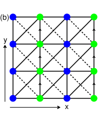
Figure 1: (Color online). Schematic of the square lattice for (a) the original model and the modified model with a staggered potential, (b) the modified model with the diagonal hopping terms. Here, the arrows represent a $\pi$ accompanying phase in the vertical hopping; The dashed lines represent a $\pi$ accompanying phase in the diagonal hopping; the blue and green filled circles represent the lattice sites of sublattices $A$ and $B$, respectively.

II Model

First, we consider the original model that consists of two sublattices denoted as $A$ and $B$, respectively, as shown in Fig.1(a). The two sublattices have the lattice spacings $2d$ and $d$ in the $x$ and $y$ directions, respectively. For sublattice $B$, along the $y$ direction, there exists an accompanying phase $\pi$ of hopping between two neighbor lattice sites. For each sublattice, the primitive lattice vectors are defined as ${\bm{a}}_{1}=(2d,0)$ and ${\bm{a}}_{2}=(0,d)$. In the following process, for simplicity, we assume $d=1$. The tight-binding Hamiltonian for the original model can be written as,

$$H_{0} = -\sum_{i\in A}[t_{x}a^{\dagger}_{i}b_{i+\hat{x}}+t_{x}a^{\dagger}_{i}b_{i-\hat{x}}$$ (1)

$$+t_{y}a^{\dagger}_{i}a_{i+\hat{y}}+t_{y}e^{-i\pi}b^{\dagger}_{i+\hat{x}}b_{i+\hat{x}+\hat{y}}+{\rm H.c.}],$$

where $a_{i}$ is the annihilation operator that destructs a particle in the Wannier state $w^{A}_{i}({\bm{r}})=w^{A}_{0}({\bm{r}}-{\bm{R}}^{A}_{i})$ located at the site $i$ in sublattice $A$, and $b_{j}$ is the annihilation operator destructing a particle in the Wannier state $w^{B}_{j}({\bm{r}})=w^{B}_{0}({\bm{r}}-{\bm{R}}^{B}_{j})$ located at the site $j$ in sublattice $B$; the subscript $i\equiv(i_{x},i_{y})$ is the coordinate for the lattice sites; $\hat{x}=(1,0)$ and $\hat{y}=(0,1)$ represent the unit vectors in the $x$ and $y$ directions, respectively; $t_{x}$ and $t_{y}$ are the amplitudes of hopping along the $x$ and $y$ directions, respectively. Without loss of generality, we assume that $t_{x}$ and $t_{y}$ are positive in the following process.

Based on the original model, we will consider two modified models with different adding terms, respectively. In the first modified model, we add a staggered potential to the original model. The total Hamiltonian can be described by $H_{1}=H_{0}+H_{s}$, where $H_{s}$ is the staggered potential Hamiltonian as

$$H_{s}=-v\sum_{i\in A}a^{\dagger}_{i}a_{i}+v\sum_{j\in B}b^{\dagger}_{j}b_{j},$$ (2)

where $v$ is the magnitude of the staggered potential. In the second modified model, we add the diagonal hopping terms to the original model, which is shown in Fig.1(b). The Hamiltonian is $H_{2}=H_{0}+H_{d}$, where $H_{d}$ is the diagonal hopping Hamiltonian as

$$H_{d} = -t_{xy}\sum_{i\in A}[a^{\dagger}_{i}b_{i+\hat{x}+\hat{y}}+a^{\dagger}_{i}b_{i-\hat{x}-\hat{y}}$$ (3)

$$-a^{\dagger}_{i}b_{i-\hat{x}+\hat{y}}-a^{\dagger}_{i}b_{i+\hat{x}-\hat{y}}+{\rm H.c.}],$$

where $t_{xy}$ is the amplitude of hopping along the diagonal direction.

For the original model and the two modified models, the lattice vectors can be expressed as ${\bm{R}}_{n}=n_{1}{\bm{a}}_{1}+n_{2}{\bm{a}}_{2}$ with $n_{1}$ and $n_{2}$ being integers. We chose a lattice site in sublattice $A$ as the origin, then the lattice sites in sublattice $A$ and sublattice $B$ can be written as ${\bm{R}}^{A}_{n}={\bm{R}}_{n}$ and ${\bm{R}}^{B}_{n}={\bm{R}}_{n}+{\bm{a}}_{1}/2$. In the reciprocal lattice, the reciprocal lattice vectors are defined as ${\bm{K}}_{m}=m_{1}{\bm{b}}_{1}+m_{2}{\bm{b}}_{2}$, where $m_{1}$ and $m_{2}$ are integers, and ${\bm{b}}_{1}=(\pi,0)$ and ${\bm{b}}_{2}=(0,2\pi)$ are the corresponding primitive reciprocal-lattice vectors. Thus, the Brillouin zone is $-\pi/2\leq k_{x}\leq\pi/2,-\pi\leq k_{y}\leq\pi$, as shown in Fig.2(b).

III Massless Dirac fermions, Moving and merging of Dirac points

In this section, we show that Dirac points exist in the original model. In the modified model with a staggered potential, the Dirac points in the Brillouin zone move when the magnitude of the staggered potential changes, and they merge when the magnitude of the staggered potential arrives at a critical value. In the modified model with the diagonal hopping terms, the two Dirac points in the Brillouin zone move towards two opposite directions as the amplitude of the diagonal hopping increases, and they never vanish or merge for any value of the amplitude of the diagonal hopping.

III.1 The original model

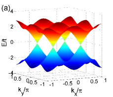
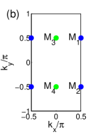
Figure 2: (Color online). (a) The dispersion relation and (b) the Brillouin zone for the original model. Here, the filled circles represent the $\Upsilon$-invariant points $M_{1},M_{2},M_{3}$ and $M_{4}$. The band degeneracy occurs at $M_{1,2}$ marked by the blue color and does not at $M_{3,4}$ marked by the green color.

For the original model, we take the Fourier’s transformation to the annihilation operators as

$${a}_{{\bm{k}}} = \frac{1}{\sqrt{N}}\sum_{i}{a}_{i}e^{-i{\bm{k}}\cdot{\bm{R}}^{A}_{i}},$$ (4)

$${b}_{{\bm{k}}} = \frac{1}{\sqrt{N}}\sum_{j}{b}_{j}e^{-i{\bm{k}}\cdot{\bm{R}}^{B}_{j}},$$ (5)

and define the two-component annihilation operator as ${\eta}_{{\bm{k}}}\equiv[{a}_{{\bm{k}}},{b}_{{\bm{k}}}]^{T}$. The total Hamiltonian $H=H_{0}+H_{1}$ can be rewritten as $H=\sum_{{\bm{k}}}{\eta}_{{\bm{k}}}^{\dagger}{\cal H}_{0}({\bm{k}}){\eta}_{{\bm{k}}}$ with

$${\cal H}_{0}({\bm{k}}) = -2t_{x}\cos k_{x}\sigma_{x}-2t_{y}\cos k_{y}\sigma_{z},$$ (6)

and $\sigma_{x}$ and $\sigma_{z}$ are the Pauli matrices.

Diagonalizing Eq.(6), we obtain the dispersion relation as

$$E_{0}({\bm{k}})=\pm\sqrt{4t_{x}^{2}\cos^{2}k_{x}+4t_{y}^{2}\cos k_{y}^{2}}.$$ (7)

The corresponding Bloch functions can be expressed as

$$\Psi^{(0)}_{\bm{k}}({\bm{r}})\equiv\left(\matrix{u^{(0)}_{1,{\bm{k}}}({\bm{r}})\cr u^{(0)}_{2,{\bm{k}}}({\bm{r}})}\right)e^{i{\bm{k}}\cdot{\bm{r}}},$$ (8)

where $u^{(0)}_{i,{\bm{k}}}({\bm{r}})=u^{(0)}_{i,{\bm{k}}}({\bm{r}}+{\bm{R}}_{n})$. In the momentum space, the Bloch function $\Psi^{(0)}_{\bm{k}}({\bm{r}})$ and eigenenergy $E_{0}({\bm{k}})$ are periodic for reciprocal lattice vectors, i.e. $\Psi^{(0)}_{\bm{k}}({\bm{r}})=\Psi^{(0)}_{{\bm{k}}+{\bm{K}}_{m}}({\bm{r}})$ and $E_{0}({\bm{k}})=E_{0}({\bm{k}}+{\bm{K}}_{m})$.

The conduction and valence bands touch at $(\pm\pi/2,\pm\pi/2)$, which are located at the boundary of the Brillouin zone as shown in Fig.2(a). Among these degenerate points, there are only two distinct ones. Near these degenerate points, the single-particle Hamiltonian (6) can be linearized as

$${h}({\bm{p}}) = 2t_{x}p_{x}\sigma_{x}\pm 2t_{y}p_{y}\sigma_{z},$$ (9)

where the signs $\pm$ representing the linearized Hamiltonian around the different touching points, respectively. Around the touching points, the quasiparticles behave like massless Dirac fermions. For these massless Dirac fermions, a chirality can be defined as Hou1

$$w=\textrm{sgn}[\det(v_{ij})]=\pm 1,$$ (10)

for a two-dimensional Hamiltonian $h({\bm{k}})=\sum_{ij}v_{ij}k_{i}\sigma_{j}$, with ${\bm{k}}$ and ${\bm{\sigma}}$ being the wave vector and the Pauli matrix in two dimensions, respectively. If we use $\sigma_{y}$ to redenote $\sigma_{z}$ in Eq.(9), the corresponding quasiparticles have a chirality $\pm 1$ as defined above. The quasiparticles are massless Dirac fermions with a chirality, so they can be considered as two-dimensional Weyl fermions. The chirality of Dirac points can be considered as a topological charge.

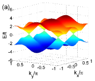
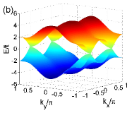
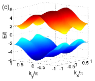
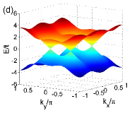
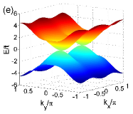
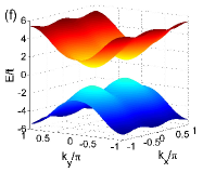
Figure 3: (Color online). The dispersion relation of the modified model with a staggered potential with $t_{x}=t_{y}=t$ and (a) $v=t_{y}$, (b) $v=2t_{y}$, (c) $v=3t_{y}$,(d) $v=-t_{y}$, (e) $v=-2t_{y}$, (f) $v=-3t_{y}$

III.2 The modified model with a staggered potential

For the modified model with a staggered potential, the Bloch Hamiltonian can be written as

$${\cal H}_{1}({\bm{k}}) = -2t_{x}\cos k_{x}\sigma_{x}-(v+2t_{y}\cos k_{y})\sigma_{z},$$ (11)

and the corresponding dispersion relation is

$$E_{1}({\bm{k}})=\pm\sqrt{4t_{x}^{2}\cos^{2}k_{x}+(v+2t_{y}\cos k_{y})^{2}}.$$ (12)

In this model, the energy dispersion relation (12) possesses Dirac points at $(\pi/2,\pm\arccos(-v/2t_{y}))$ in the Brillouin zone for $|v|<2t_{y}$, as shown Fig.(3)(a) and (d). We find that the two distinct Dirac points move as $v$ changes. For the positive $v$, with increasing $v$, the two Dirac points move away from each other. When $v=0$, the Dirac points are located at points $(\pi/2,\pm\pi/2)$ as shown in Fig.2(a). When $v$ changes from $0$ to $t_{y}$, the two distinct Dirac points move to $(\pi/2,\pm 2\pi/3)$, respectively, as shown in 3(a). When $v$ arrives at $2t_{y}$, the two Dirac points move to $(\pi/2,\pm\pi)$, which are the same point on the boundary of the Brillouin zone as shown in Fig.3(b), that is to say, the Dirac points merge. If one continues to increase $v$ to $v>2t_{y}$, a gap opens, as shown in Fig.3 (c). Then the system turns into an insulator. For the negative $v$, with increasing $|v|$, the two Dirac points move towards each other. When $v$ changes from $0$ to $-t_{y}$, the two distinct Dirac points move to $(\pi/2,\pm\pi/3)$, respectively, as shown in 3(d). When $v$ arrives at $-2t_{y}$, the two Dirac points merge at the point $(\pi/2,0)$ as shown in 3(e). When $v$ is less than $-2t_{y}$, a gap opens and the systems turns into an insulator, as shown in Fig.3(f).

The above merging process of Dirac points can be interpreted from the topological view. Two Dirac points have opposite chirality, that is to say, they have opposite topological charges. As long as the band touching points are protected by a symmetry, the topological charges can not be destroyed, and the system is a topological semimetal. However, when the Dirac points with opposite topological charges meet, they merge and the opposite topological charges annihilate each other.Volovik A further increase of $|v|$ makes a gap open and the system turns into an insulator.

III.3 The modified model with the diagonal hopping terms

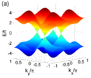
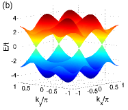
Figure 4: (color online). The dispersion relation of the modified model with the diagonal hopping terms with $t_{x}=t_{y}=t$ and (a) $t_{xy}=t_{x}$, (b) $t_{xy}=-t_{x}$.

For the modified model with the diagonal hopping terms, the Bloch Hamiltonian can be expressed as

$${\cal H}_{2}({\bm{k}}) = -(2t_{x}\cos k_{x}+4t_{xy}\sin k_{x}\sin k_{y})\sigma_{x}$$ (13)

$$-2t_{y}\cos k_{y}\sigma_{z},$$

and the corresponding dispersion relation is

$$E_{2}({\bm{k}})=\pm\sqrt{(2t_{x}\cos k_{x}+4t_{xy}\sin k_{x}\sin k_{y})^{2}+4t_{y}^{2}\cos^{2}k_{y}}.$$

In this model, the bands touch at the points $(-\arctan(t_{x}/2t_{xy}),\pi/2)$ and $(\arctan(t_{x}/2t_{xy}),-\pi/2)$ in the Brillouin zone. Near these degenerate points, the dispersion relation is linear. Thus, these points are also Dirac points and have a chirality defined above. Compared with the original model, the Dirac points have a shift in the Brillouin zone. For the case $t_{xy}/t_{x}>0$, with increasing $|t_{xy}|$, the Dirac point in the $k_{y}>0$ half part of the Brillouin zone moves towards the $x$ direction, while the Dirac point in the $k_{y}<0$ half part of the Brillouin zone moves towards the negative $x$ direction as shown in Fig.4(a). When the parameter $|t_{xy}|$ approaches infinity, the Dirac points move asymptotically to the $k_{x}=0$ line. For the case of $t_{xy}/t_{x}<0$, the Dirac points have similar shifts but with the opposite directions compared with the case of $t_{xy}/t_{x}>0$. That is to say, the Dirac point in the $k_{y}>0$ half part of the Brillouin zone moves towards the negative $x$ direction, while the Dirac point in the $k_{y}<0$ half part of the Brillouin towards the $x$ direction as shown in Fig.4(b). For any value of the parameter $t_{xy}$, the system remains gapless and the Dirac points never merge, which is different from the modified model with a staggered potential.

IV Explanation from hidden symmetry protection

In this section, we prove that the Dirac points are protected by a kind of hidden symmetry in the original model. In the two modified models, the additive terms violate the hidden symmetry respected by the original model. Thus, we develop a mapping method to find hidden symmetries evolving with the parameters for the two modified model. We explain the moving of Dirac points in the two modified models by the evolution of the hidden symmetries along with the variation of the parameters, and we explain the merging of Dirac points in the modified model with a staggered potential by the disappearance of the hidden-symmetry-invariant points in the Brillouin zone.

IV.1 The original model

The original model supports the existence of massless Dirac fermions with the Dirac points located at $(\pi/2,\pm\pi/2)$ in the Brillouin zone. We will show that the band degeneracies at the Dirac points are protected by a hidden symmetry. Here, we define a hidden symmetry with the operator as follows,

$$\Upsilon=(e^{i\pi})^{i_{y}}\sigma_{x}KT_{{{\bm{a}}}_{1}/2},$$ (15)

where $T_{{\bm{a}}_{1}/2}=\{E|{\bm{a}}_{1}/2\}$ is a translation operator that moves the lattice by ${\bm{a}}_{1}/2$ along the $x$ direction, $K$ is the complex conjugate operator, $\sigma_{x}$ is the Pauli matrix representing sublattice exchange, and $(e^{i\pi})^{i_{y}}$ is a local $U(1)$ gauge transformation. Obviously, the hidden symmetry operator $\Upsilon$ is an antiunitary operator. The corresponding inverse operator is $\Upsilon^{-1}=(e^{i\pi})^{i_{y}}\sigma_{x}KT_{{{\bm{a}}}_{1}/2}^{-1}$. It is easy to verify that the Hamiltonian of the original model is invariant under the hidden symmetry transformation, i.e. $H_{0}=\Upsilon H_{0}\Upsilon^{-1}$.

The hidden symmetry operator $\Upsilon$ acts on the Bloch functions (8) as follows

$$\Upsilon\Psi^{(0)}_{{\bm{k}}}({\bm{r}}) = \left(\matrix{u^{(0)*}_{2,{\bm{k}}}({\bm{r}}-{\bm{a}}_{1}/2)e^{ik_{x}}\cr u^{(0)*}_{1,{\bm{k}}}({\bm{r}}-{\bm{a}}_{1}/2)e^{ik_{x}}}\right)e^{-i[k_{x}x+(k_{y}-\pi)y]}$$ (16)

$$= {\Psi^{(0)}_{{\bm{k}}^{\prime}}}^{\prime}({\bm{r}}).$$

Because $\Upsilon$ is the symmetry operator for the original model, ${\Psi^{(0)}_{{\bm{k}}^{\prime}}}^{\prime}({\bm{r}})$ must be a Bloch wave function of the original model. Thus, we obtain $u^{(0)}_{1,{\bm{k}}^{\prime}}({\bm{r}})=u^{(0)*}_{2,{\bm{k}}}({\bm{r}}-{\bm{a}}_{1}/2)e^{ik_{x}}$ and $u^{(0)}_{2,{\bm{k}}^{\prime}}({\bm{r}})=u^{(0)*}_{1,{\bm{k}}}({\bm{r}}-{\bm{a}}_{1}/2)e^{ik_{x}}$, $k^{\prime}_{x}=-k_{x}$ and $k^{\prime}_{y}=\pi-k_{y}$. The square of the hidden symmetry operator is

$$\Upsilon^{2}=T_{{{\bm{a}}}_{1}},$$ (17)

where $T_{{\bm{a}}_{1}}=\{E|{\bm{a}}_{1}\}$. Therefore, we have

$$\Upsilon^{2}\Psi^{(0)}_{{\bm{k}}}({\bm{r}})=T_{{\bm{a}}_{1}}\Psi^{(0)}_{{\bm{k}}}({\bm{r}})=e^{-2ik_{x}}\Psi^{(0)}_{{\bm{k}}}({\bm{r}}).$$ (18)

From Eqs. (8) and (16), it is easy to show that the operator $\Upsilon$ has the following effect when acting on the wave vector ${\bm{k}}$:

$$\Upsilon:{\bm{k}}=(k_{x},k_{y})\rightarrow{\bm{k}}^{\prime}=(-k_{x},-k_{y}+\pi).$$ (19)

If ${\bm{k}}^{\prime}={\bm{k}}+{\bm{K}}_{m}$, then we can say that ${\bm{k}}$ is an invariant point under the hidden symmetry transformation. In the Brillouin zone, the $\Upsilon$-invariant points are $M_{1,2}=(\pi/2,\pm\pi/2)$ and $M_{3,4}=(0,\pm\pi/2)$ as shown in Fig.2(b). For a $\Upsilon$-invariant point $M_{i}$, we have $\Upsilon\Psi^{(0)}_{M_{i}}({\bm{r}})={\Psi^{(0)}_{M_{i}}}^{\prime}({\bm{r}})$. Thus, $\Psi^{(0)}_{M_{i}}({\bm{r}})$ and ${\Psi^{(0)}_{M_{i}}}^{\prime}({\bm{r}})$ are both the eigenstates of Hamiltonian $H_{0}$ and have the same eigenenergy $E_{0}(M_{i})$. Considering Eq.(17), we have $\Upsilon^{2}\Psi^{(0)}_{M_{i}}({\bm{r}})=T_{{\bm{a}}_{1}}\Psi^{(0)}_{M_{i}}({\bm{r}})=e^{-2iM_{ix}}\Psi^{(0)}_{M_{i}}({\bm{r}})$, where $M_{ix}$ is the $x$ component of $M_{i}$. We define $(\psi,\varphi)$ as the inner product of the two wave functions $\psi$ and $\varphi$. The antiunitary operator $\Upsilon$ has the property that $(\Upsilon\psi,\Upsilon\varphi)=(\psi,\varphi)^{*}=(\varphi,\psi)$. Therefore, we have

$$({\Psi^{(0)}_{M_{i}}}^{\prime},\Psi^{(0)}_{M_{i}}) = (\Upsilon\Psi^{(0)}_{M_{i}},\Upsilon{\Psi^{(0)}_{M_{i}}}^{\prime})=(\Upsilon\Psi^{(0)}_{M_{i}},\Upsilon^{2}\Psi^{(0)}_{M_{i}})$$ (20)

$$= e^{-2iM_{ix}}({\Psi^{(0)}_{M_{i}}}^{\prime},\Psi^{(0)}_{{M_{i}}}).$$

Substituting the concrete $\Upsilon$-invariant points $M_{i}$, we have $\Upsilon^{2}=-1$ at $M_{1,2}$, while $\Upsilon^{2}=-1$ at $M_{3,4}$. Then we obtain the solution $({\Psi^{(0)}_{M_{i}}}^{\prime},\Psi^{(0)}_{M_{i}})=0$ at $M_{1,2}$, i.e., ${\Psi^{(0)}_{M_{i}}}^{\prime}$ and $\Psi^{(0)}_{M_{i}}$ are orthogonal to each other, while $({\Psi^{(0)}_{M_{i}}}^{\prime},\Psi^{(0)}_{M_{i}})$ is unconstrained for Eq.(20) at $M_{3,4}$. Therefore, we arrive at the conclusion that the system must be degenerate at points $M_{1,2}$ in the Brillouin zone, which are just the positions where the Dirac points are located. We can conclude that the two Dirac points are protected by the hidden symmetry $\Upsilon$.

IV.2 The modified model with a staggered potential

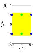
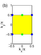
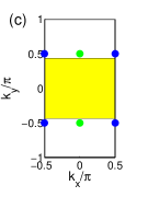
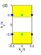
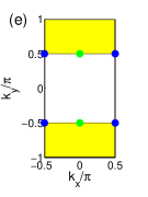
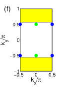
Figure 5: (color online). The mapping of the Brillouin zone of the modified model with a staggered potential for (a) $v=t_{y}$, (b) $v=2t_{y}$, (c) $v=3t_{y}$,(d) $v=-t_{y}$, (e) $v=-2t_{y}$, and (f) $v=-3t_{y}$ into the Brillouin zone of the original model, respectively. The area surrounded by the solid line is the Brillouin zone of the original model. The yellow shaded area is the image of the Brillouin zone of the modified model with a staggered potential mapping into the Brillouin zone of the original model. The filled circles represent the $\Upsilon$-invariant points in the Brillouin zone of the original model.

For the modified model with a staggered potential, the total Hamiltonian violates the hidden symmetry, i.e., $[\Upsilon,H_{1}]\neq 0$. However, Dirac points still exist and just move to other points in the Brillouin zone before the magnitude of the staggered potential $v$ arrives at the critical value. Due to the von Neumann-Wigner theorem, in the two-dimensional lattice, the band degeneracy must be protected by a symmetry.vNW ; Balents After the hidden symmetry $\Upsilon$ is violated, which symmetry protects the band degeneracy at the Dirac points? In the following, we will explain which symmetry is responsible for that.

Now we define a mapping as

$$\Omega_{v}:({\bm{k}},\mathcal{H}_{1}({\bm{k}}),\Psi^{(1)}_{\bm{k}}({\bm{r}}))\mapsto({\bm{K}},\mathcal{H}_{0}({\bm{K}}),\Psi^{(0)}_{{\bm{K}}}({\bm{r}})),$$ (21)

which maps the Bloch Hamiltonian (11) into the form as

$${\cal H}_{0}({\bm{K}}) = -2t_{x}^{\prime}\cos K_{x}\sigma_{x}-2t_{y}^{\prime}\cos K_{y}\sigma_{z},$$ (22)

where $t_{x}^{\prime}=t_{x}$ and $t_{y}^{\prime}=t_{y}+|v|/2$. Eq.(22) is just the Bloch Hamiltonian (6) of the original model except for the different notations of the parameters. Eq.(22) must have the $\Upsilon$-invariant points in Brillouin zone as $M_{1,2}=(\pi/2,\pm\pi/2)$ and $M_{3,4}=(0,\pm\pi/2)$ as shown in Fig.2(b). For the wave vectors, the transformation (21) is explicitly written as

$$K_{x} = k_{x},\ \mbox{for}\ k_{x}\in[-\pi/2,\pi/2],$$ (23)

$$K_{y} = \left\{\matrix{-\arccos\left(\frac{v+2t_{y}\cos k_{y}}{|v|+2t_{y}}\right),&k_{y}\in[-\pi,0]\cr\arccos\left(\frac{v+2t_{y}\cos k_{y}}{|v|+2t_{y}}\right),&k_{y}\in[0,\pi]}\right.,$$ (24)

and for the Bloch functions, it can be written as

$$\Omega_{v}\Psi^{(1)}_{\bm{k}}({\bm{r}})=\Psi^{(0)}_{\bm{K}}({\bm{r}}),$$ (25)

where $\Psi^{(0)}_{\bm{K}}({\bm{r}})$ is the Bloch function of the original model. The shift from ${\bm{k}}$ to ${\bm{K}}$ after the transformation is ${\bm{K}}-{\bm{k}}=(0,\delta_{k_{y}})$ with

$$\delta_{k_{y}}=\left\{\matrix{-k_{y}-\arccos\left(\frac{v+2t_{y}\cos k_{y}}{|v|+2t_{y}}\right),&k_{y}\in[-\pi,0]\cr-k_{y}+\arccos\left(\frac{v+2t_{y}\cos k_{y}}{|v|+2t_{y}}\right),&k_{y}\in[0,\pi]}\right..$$ (26)

The transformation (23) implies that $k_{x}$ mapping into $K_{x}$ is just an equivalence. From Eq.(24), we note that the mapping $k_{y}\rightarrow K_{y}$ is more complicated. When $v$ is positive, $\Omega_{v}$ maps the range $[-\pi,\pi]$ for $k_{y}$ into the range $[-\arccos((v-2t_{y})/(|v|+2t_{y})),\arccos((v-2t_{y})/(|v|+2t_{y}))]$ for $K_{y}$. For the points located on the top and bottom boundaries of the Brillouin zone of the modified model with a staggered potential, due to the equivalence between points on the boundary of the Brillouin zone, the mapping is not one-to-one. For the interior points of the Brillouin zone of the modified model with a staggered potential, the mapping is continuous and one-to-one. On the whole, the mapping is not surjective for non-vanishing $v$, i.e., the whole Brillouin zone of the modified model with a staggered potential maps into part of the Brillouin zone of the original model, as shown in Figs.5(a),(b) and (c). When $v$ is negative, $\Omega_{v}$ maps the ranges $[-\pi,0]$ and $[0,\pi]$ for $k_{y}$ into the ranges $[-\pi,-\arccos((v+2t_{y})/(|v|+2t_{y}))]$ and $[\arccos((v+2)/(|v|+2t_{y})),\pi]$ for $K_{y}$, respectively. Especially, $\Omega_{v}$ maps $k_{y}=0$ into $K_{y}=\pm\arccos((v+2)/(|v|+2t_{y}))$, which is not one-to-one. In the interior part of each range, the mapping is continuous and one-to-one. On the whole, the mapping is not surjective for non-vanishing $v$, as shown in Figs.5(d),(e) and (f).

We define a new hidden symmetry as $\Lambda_{v}=\Omega_{v}^{-1}\Upsilon\Omega_{v}$, which consists of three operators acting in order on the wave vector and the Bloch functions. Since the operator $\Lambda_{v}$ depends on $v$, the hidden symmetry evolves along with the magnitude of the staggered potential. When $v=0$, the operator $\Lambda_{v}$ returns to $\Upsilon$. For the wave vectors, the operation is performed as $\Omega_{v}:{\bm{k}}\rightarrow{\bm{K}}$, $\Upsilon:{\bm{K}}\rightarrow{\bm{K}}^{\prime}$ and $\Omega_{v}^{-1}:{\bm{K}}^{\prime}\rightarrow{\bm{k}}^{\prime}$. Considering the explicit form of these transformations as Eqs.(19),(23) and (24), we have

$$\Lambda_{v}:{\bm{k}}=(k_{x},k_{y})\rightarrow{\bm{k}}^{\prime}=(-k_{x},-k_{y}-\delta_{k_{y}}-\delta_{k^{\prime}_{y}}+\pi).$$ (27)

If the condition ${\bm{k}}^{\prime}={\bm{k}}+{\bm{K}}_{m}$ is satisfied, then we can say that ${\bm{k}}$ is a $\Lambda_{v}$-invariant point in the Brillouin zone of the modified model with a staggered potential. Through Eqs.(26) and (27), we can show that the $\Lambda_{v}$-invariant points in the Brillouin zone of the modified model with a staggered potential have the form as $P_{1,2}=(\pi/2,\pm\arccos(-v/2t_{y}))$ and $P_{3,4}=(0,\pm\arccos(-v/2t_{y}))$. We find that when $|v/t_{y}|=2$, $\Lambda_{v}$-invariant points $P_{1}$ and $P_{2}$ are located at the $k_{y}=0$ line or the top and bottom boundaries of the Brillouin zone of the modified model with a staggered potential, so they meet together. That is so for $P_{3}$ and $P_{4}$. However, when $|v/t_{y}|>2$, there is no solution for $\Lambda_{v}$-invariant points, i.e. there does not exist any $\Lambda_{v}$-invariant point.

For the square of the operator $\Lambda_{v}$, we have $\Lambda_{v}^{2}=\Omega_{v}^{-1}\Upsilon^{2}\Omega_{v}$. The hidden symmetry operator $\Lambda_{v}$ acting on the Bloch function $\Psi^{(1)}_{\bm{k}}({\bm{r}})$ twice successively has following the effect:

$$\Lambda_{v}^{2}\Psi^{(1)}_{\bm{k}}({\bm{r}})=e^{-2ik_{x}}\Psi^{(1)}_{\bm{k}}({\bm{r}}),$$ (28)

which can be derived from Eqs.(18), (23), (24) and (25). Since $\Lambda_{v}$ is an antiunitary operator, similar to Eq.(20), we have the following equation

$$({\Psi^{(1)}_{P_{i}}}^{\prime},\Psi^{(1)}_{P_{i}}) = (\Lambda_{v}\Psi^{(1)}_{P_{i}},\Lambda_{v}{\Psi^{(1)}_{P_{i}}}^{\prime})=(\Lambda_{v}\Psi^{(1)}_{P_{i}},\Lambda_{v}^{2}\Psi^{(1)}_{P_{i}})$$ (29)

$$= e^{-2iP_{ix}}({\Psi^{(1)}_{P_{i}}}^{\prime},\Psi^{(1)}_{P_{i}}).$$

From Eq.(28), we have $\Lambda_{v}^{2}=-1$ at $\Lambda_{v}$-invariant points $P_{1}$ and $P_{2}$, and $\Lambda_{v}^{2}=1$ at $\Lambda_{v}$-invariant points $P_{3}$ and $P_{4}$. Therefore, we have the solution $({\Psi^{(1)}_{P_{i}}},\Psi^{(1)}_{P_{i}})=0$ at the $\Lambda_{v}$-invariant points $P_{1}$ and $P_{2}$. We conclude that the bands must be degenerate at the points $P_{1}$ and $P_{2}$ but are not at the points $P_{3}$ and $P_{4}$, which is consistent with the dispersion relation calculated previously. That is to say, the Dirac points at $P_{1}$ and $P_{2}$ are protected by the hidden symmetry $\Lambda_{v}$. Since $\Lambda_{v}$ depends on the magnitude of the staggered potential $v$, the hidden symmetry protected degenerate points $P_{1}$ and $P_{2}$ evolve along with changing of the parameter $v$ for $|v/t_{y}|<2$. For the case $|v/t_{y}|=2$, $P_{1}$ and $P_{2}$ are the same points, so the Dirac points merge. When $|v/t_{y}|>2$, the $\Lambda_{v}$-invariant points $P_{1}$ and $P_{2}$ do not exist, so a gap opens.

We can interpret the hidden symmetry protection in a more intuitive way. Although the modified model with a staggered potential violates the hidden symmetry $\Upsilon$, the operator $\Omega_{v}$ can map the Bloch Hamiltonian (11) into the Bloch Hamiltonian (6), which is just the Bloch Hamiltonian of the original model. However, the mapping $\Omega_{v}$ is not surjective. That is, the Brillouin zone of the modified model with a staggered model maps into part of the Brillouin zone of the original model as shown in Fig.5. When $|v/t_{y}|<2$, the image of the Brillouin zone of the modified model with a staggered model includes the $\Upsilon$-invariant points in the Brillouin zone of the original model as shown in Fig.5(a) and (d). There always exist four points in the Brillouin zone of the modified model with a staggered model mapping into the four $\Upsilon$-invariant points in the Brillouin zone of the original model. When $|v/t_{y}|=2$, the two points on the boundary or $k_{y}=0$ line of the Brillouin zone of the modified model with a staggered potential map into the four $\Upsilon$-invariant points in the Brillouin zone of the original model, as shown in Fig.5(b) and (e). The two Dirac points meet and merge. When $|v/t_{y}|>2$, the Brillouin zone of the modified model with a staggered potential maps into part of the Brillouin zone of the original model, which does not include the $\Upsilon$-invariant points as shown in Fig.5(c) and (f). This is to say, there does not exist any point in the Brillouin zone of the modified model with a staggered potential that can map into the $\Upsilon$-invariant points in the Brillouin zone of the original model. Thus, there are no symmetries to support the existence fo Dirac points.

IV.3 The modified model with the diagonal hopping terms

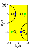
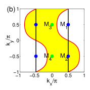
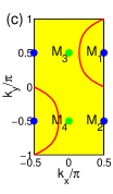
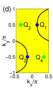
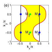
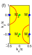
Figure 6: (color online). The mapping of the Brillouin zone of the modified model with the diagonal hopping terms into the Brillouin zone of the original model. (a) The Brillouin zone of the modified model with the diagonal hopping terms, (b) the image of mapping of the modified model with the diagonal hopping terms in the momentum space of the original model, and (c) the image of mapping of the modified model with the diagonal hopping terms restricted in the Brillouin zone of the original model for $t_{xy}=t_{x}$; (d) the Brillouin zone of the modified model with the diagonal hopping terms, (e) the image of mapping of the modified model with the diagonal hopping terms in the momentum space of the original model, and (f) the image of mapping of the modified model with the diagonal hopping terms restricted in the Brillouin zone of the original model for $t_{xy}=-t_{x}$. Here, $Q_{i}$ denotes the $\Lambda^{\prime}_{t_{xy}}$-invariant points in the Brillouin zone of the modified model with the diagonal hopping terms, and $M_{i}$ denotes the $\Upsilon$-invariant points in the Brillouin zone of the original model. The black curves in (a) and (d) map into the left and right boundary of the Brillouin zone of the original model.

In the modified model with the diagonal hopping terms, the hidden symmetry $\Upsilon$ respected by the original model is violated due to the additive diagonal hopping terms. However, in this model, the Dirac points do not vanish, so there must be some symmetry to protect them.

Similarly, we define a mapping from the modified model with the hopping terms to the original model as

$$\Omega^{\prime}_{t_{xy}}:({\bm{k}},\mathcal{H}_{2}({\bm{k}}),\Psi^{(2)}_{\bm{k}}({\bm{r}}))\mapsto({\bm{K}},\mathcal{H}_{0}({\bm{K}}),\Psi^{(0)}_{{\bm{K}}}({\bm{r}})),$$ (30)

where $\Psi^{(2)}_{\bm{k}}({\bm{r}})$ is the Bloch function for the modified model with the diagonal hopping terms. Toward that end, we first rewrite the Bloch Hamiltonian (13) as

$${\cal H}_{2}({\bm{k}}) = -2T_{k_{y}}\cos(k_{x}-\alpha_{k_{y}})\sigma_{x}-2t_{y}\cos k_{y}\sigma_{z}$$ (31)

where the parameter $T_{k_{y}}$ is defined as $T_{k_{y}}=\sqrt{t_{x}^{2}+4t_{xy}^{2}\sin^{2}k_{y}}$, which depends on $k_{y}$; the parameter $\alpha_{k_{y}}$ also depends on $k_{y}$ and is defined by $\alpha_{k_{y}}=\arctan(2t_{xy}\sin k_{y}/t_{x})$. If we suppose that the mapping $\Omega^{\prime}_{t_{xy}}$ has the effect as

$$\Omega^{\prime}_{t_{xy}}:(k_{x},k_{y})\rightarrow(K_{x},K_{y})=(k_{x}-\alpha_{k_{y}},k_{y}),$$ (32)

and $T_{k_{y}}\rightarrow t_{x}^{\prime}=T_{k_{y}}\cos\alpha_{k_{y}}=t_{x}$ and $t_{y}\rightarrow t_{y}^{\prime}=t_{y}$, then ${\cal H}_{2}({\bm{k}})$ maps into ${\cal H}_{0}({\bm{K}})$ as

$${\cal H}_{0}({\bm{K}}) = -2t_{x}^{\prime}\cos K_{x}\sigma_{x}-2t_{y}^{\prime}\cos K_{y}\sigma_{z},$$ (33)

which is just the Bloch Hamiltonian (6) except for the different notations of the parameters. For the Bloch functions, we have

$$\Omega^{\prime}_{t_{xy}}\Psi^{(2)}_{{\bm{k}}}({\bm{r}})=\Psi^{(0)}_{{\bm{K}}}({\bm{r}}).$$ (34)

We define a new hidden symmetry as $\Lambda^{\prime}_{t_{xy}}={\Omega^{\prime}}^{-1}_{t_{xy}}\Upsilon\Omega^{\prime}_{t_{xy}}$. For the wave vectors, the operation is performed as $\Omega^{\prime}_{t_{xy}}:{\bm{k}}\rightarrow{\bm{K}}$, $\Upsilon:{\bm{K}}\rightarrow{\bm{K}}^{\prime}$, ${\Omega^{\prime}}_{t_{xy}}^{-1}:{\bm{K}}^{\prime}\rightarrow{\bm{k}}^{\prime}$. Considering the explicit form of these transformations as Eqs.(19) and (32), we have

$$\Lambda^{\prime}_{t_{xy}}:{\bm{k}}=(k_{x},k_{y})\rightarrow{\bm{k}}^{\prime}=(-k_{x}+\alpha_{k_{y}}+\alpha_{k_{y}^{\prime}},-k_{y}+\pi)$$ (35)

If the condition ${\bm{k}}^{\prime}={\bm{k}}+{\bm{K}}_{m}$ is satisfied, then we can say that ${\bm{k}}$ is a $\Lambda^{\prime}_{t_{xy}}$-invariant point in the Brillouin zone of the modified model with the diagonal hopping terms. In this model, the $\Lambda^{\prime}_{t_{xy}}$-invariant points in the Brillouin zone are $Q_{1}=(-\arctan(t_{x}/2t_{xy}),\pi/2)$, $Q_{2}=(\arctan(t_{x}/2t_{xy}),-\pi/2)$, $Q_{3}=(\arctan(2t_{xy}/t_{x}),\pi/2)$ and $Q_{4}=(-\arctan(2t_{xy}/t_{x}),-\pi/2)$, as shown in Fig.6 (a) for the case of $t_{xy}/t_{x}>0$ and Fig.6(d) for the case of $t_{xy}/t_{x}<0$.

For the square of the operator $\Lambda^{\prime}_{t_{xy}}$, we have ${\Lambda^{\prime}}_{t_{xy}}^{2}={\Omega^{\prime}}_{t_{xy}}^{-1}\Upsilon^{2}\Omega^{\prime}_{t_{xy}}={\Omega^{\prime}}_{t_{xy}}^{-1}T_{{\bm{a}}_{1}}\Omega^{\prime}_{t_{xy}}$. The hidden symmetry operator $\Lambda^{\prime}_{t_{xy}}$ acting on the Bloch function $\Psi^{(2)}_{{\bm{k}}}({\bm{r}})$ twice successively has the effect as

$${\Lambda^{\prime}}_{t_{xy}}^{2}\Psi^{(2)}_{{\bm{k}}}({\bm{r}})=e^{-2i(k_{x}-\alpha_{k_{y}})}\Psi^{(2)}_{{\bm{k}}}({\bm{r}})$$ (36)

which can be derived from Eqs.(18) and (32). Since $\Lambda^{\prime}_{t_{xy}}$ is an antiunitary operator, similar to Eq.(20), we have the following equation

$$({\Psi^{(2)}_{Q_{i}}}^{\prime},\Psi^{(2)}_{Q_{i}}) = (\Lambda^{\prime}_{t_{xy}}\Psi^{(2)}_{Q_{i}},\Lambda^{\prime}_{t_{xy}}{\Psi^{(2)}_{Q_{i}}}^{\prime})=(\Lambda^{\prime}_{t_{xy}}\Psi^{(2)}_{Q_{i}},{\Lambda^{\prime}_{t_{xy}}}^{2}\Psi^{(2)}_{Q_{i}})$$ (37)

$$= e^{-2i(Q_{ix}-\alpha_{Q_{iy}})}({\Psi^{(2)}_{Q_{i}}}^{\prime},\Psi^{(2)}_{Q_{i}}).$$

From Eq.(36), we can obtain ${\Lambda^{\prime}}^{2}_{t_{xy}}=-1$ at the $\Lambda^{\prime}_{t_{xy}}$-invariant points $Q_{1}$ and $Q_{2}$, and ${\Lambda^{\prime}}^{2}_{t_{xy}}=1$ at the $\Lambda^{\prime}_{t_{xy}}$-invariant points $Q_{3}$ and $Q_{4}$. Therefore, we have the solution $({\Psi^{(2)}_{Q_{i}}}^{\prime},\Psi^{(2)}_{Q_{i}})=0$ at the $\Lambda^{\prime}_{t_{xy}}$-invariant points $Q_{1}$ and $Q_{2}$. We conclude that the bands must be degenerate at the points $Q_{1}$ and $Q_{2}$ while the band degeneracy is not guaranteed at the points $Q_{3}$ and $Q_{4}$, which is consistent with the dispersion relation calculated previously. That is to say, the Dirac points at $Q_{1}$ and $Q_{2}$ are protected by the hidden symmetry $\Lambda^{\prime}_{t_{xy}}$. The hidden symmetry $\Lambda^{\prime}_{t_{xy}}$ evolves along with the parameter $t_{xy}$. It is easy to find that when $t_{xy}=0$, the hidden symmetry operator $\Lambda^{\prime}_{t_{xy}}$ returns to the operator $\Upsilon$ and the degenerate points $Q_{1}$ and $Q_{2}$ are just the points $M_{1}$ and $M_{2}$. When $t_{xy}$ changes, the degenerate points $Q_{1}$ and $Q_{2}$ move towards opposite directions, respectively. When $t_{xy}$ approaches infinity, the degenerate points approach the $k_{y}=0$ line from two sides, respectively. For any value of the parameter $t_{xy}$, the degenerate points $Q_{1}$ and $Q_{2}$ do not merge and no gap opens. All these conclusions are consistent with the dispersion relation calculated previously.

We can interpret the above conclusions from the mapping of the Brillouin zone of the modified model with the diagonal hopping terms to the Brillouin zone of the original model, which is shown in Figs.6(a),(b),(c) for the case of $t_{xy}/t_{x}>0$ and Figs.6(d),(e),(f) for the case of $t_{xy}/t_{x}<0$. Figs.6(a) and (d) show the Brillouin zone of the modified model with the diagonal hopping terms. Figs.6(b) and (e) show the image of the mapping $\Omega^{\prime}_{t_{xy}}$ of the Brillouin zone of the modified model with the diagonal hopping terms in the momentum space of the original model. If the image of the mapping $\Omega^{\prime}_{t_{xy}}$ is restricted in the Brillouin zone of the original model, it is like that shown in Figs.6 (c) and (f). It is easy to find that the mapping $\Omega^{\prime}_{t_{xy}}$ just shifts the points in the Brillouin zone along the $x$ direction as shown in Figs.6(b) and (e). The mapping $\Omega^{\prime}_{t_{xy}}$ is one-to-one and surjective, which can be found from Figs.6(c) and (d). Specifically, the left and right boundaries of the Brillouin zone of the modified model with the diagonal hopping terms as shown in Figs.6 (a) and (b) map into the red solid lines in the Brillouin zone of the original model as shown in Figs.6(c) and (f). The black curved lines in the Brillouin zone of the modified model with the diagonal hopping terms as shown in Figs.6 (a) and (b) map into the left and right boundary of the Brillouin zone of the original model, where the $\Upsilon$-invariant points $M_{1}$ and $M_{2}$ are located. The $\Lambda^{\prime}_{t_{xy}}$-invariant points $Q_{i}(i=1,2,3,4)$ in the Brillouin zone of the modified model with the diagonal hopping terms map into the $\Upsilon$-invariant points $M_{i}(i=1,2,3,4)$ in the Brillouin zone of the original model. Since the mapping is surjective, there always exist points $Q_{1}$ and $Q_{2}$ in the Brillouin zone of the modified model with the diagonal hopping terms mapping into the $\Upsilon$-invariant points $M_{1}$ and $M_{2}$ in the Brillouin zone of the original model. Therefore, the Dirac points always are protected by a hidden symmetry and no gap opens for any value of the parameter $t_{xy}$. Because the corresponding hidden symmetry $\Lambda^{\prime}_{t_{xy}}$ evolves along with the parameter $t_{xy}$, the Dirac points move as the parameter $t_{xy}$ changes.

V Conclusion

In summary, we have studied the original model, a fermionic square lattice with only the horizontal and vertical hopping terms, and the two modified models with a staggered potential and the diagonal hopping terms, respectively. All three models support the existence of massless Dirac fermions. In the original model, there are two Dirac points in the Brillouin zone, which are protected by a hidden symmetry. In the modified model with a staggered potential, the two Dirac points move away from or approach each other with increasing of the magnitude of the staggered potential. When the magnitude arrives at a critical value, the two Dirac points merge at the $k_{y}=0$ line or the $k_{y}=\pi$ line which is determined by the sign of the staggered potential. When the magnitude of the staggered potential is greater than the critical value, a gap opens, and the system becomes an insulator. In the modified model with the diagonal hopping terms, the two Dirac points in the Brillouin move with increasing amplitude of the diagonal hopping in two opposite directions, respectively. But the Dirac points never vanish and the system is always gapless for any amplitude of the diagonal hopping. For the two modified models, we have developed a mapping method that maps the modified models into the original model, to find hidden symmetries evolving with the parameters. The moving of the Dirac points in the Brillouin zone for the two modified models can be explained by the evolution of the hidden symmetries along with the parameters. The merging of Dirac points in the modified model with a staggered potential can also be explained by the disappearance of the hidden-symmetry-invariant points in the Brillouin zone when the parameter is beyond the critical value. The original model can be realized experimentally and detected in an optical lattice with laser-assisted tunneling as proposed in Reference [Hou2, ]. Based on the original model, two modified models can also be realized with the existing techniques on optical lattices. The topological charge at Dirac points can be detected by the interferometric approach.Abanin

References

• (1) K.S. Novoselov, A.K. Geim, S.V. Morozov, D. Jiang, Y. Zhang, S.V. Dubonos, I.V. Grigorieva, and A. A. Firsov, Science 306, 666 (2004).
• (2) K.S. Novoselov, A.K. Geim, S.V. Morozov, D. Jiang, M.I. Katsnelson, I.V. Grigorieva, S.V. Dubonos, and A.A. Firsov, Nature (London) 438, 197 (2005).
• (3) Y. Zhang, Y.W. Tan, H.L. Stormer, and Philip Kim, Nature (London) 438, 201 (2005).
• (4) V. P. Gusynin and S. G. Sharapov, Phys. Rev. Lett. 95, 146801 (2005).
• (5) G. Li and E. Y. Andrei, Nat. Phys. 3, 623 (2007).
• (6) J.M. Hou, W.X. Yang and X.J. Liu, Phys. Rev. A 79, 043621 (2009).
• (7) S.L. Zhu, B. Wang, and L.M. Duan, Phys. Rev. Lett. 98, 260402 (2007).
• (8) N. Goldman, A. Kubasiak, A. Bermudez, P. Gaspard, M. Lewenstein, and M. A. Martin-Delgado, Phys. Rev. Lett. 103, 035301 (2009).
• (9) D. Bercioux, D. F. Urban, H. Grabert, and W. HΓ€usler, Phys. Rev. A 80, 063603 (2009).
• (10) N. Goldman, E. Anisimovas, F. Gerbier, P. Γ–hberg, I. B. Spielman, G. JuzeliΕ«nas, New J. Phys. 15, 013025 (2013).
• (11) L. Tarruell, D. Greif, T. Uehlinger, G. Jotzu, and T. Esslinger, Nature (London) 483, 302 (2012).
• (12) L. Fu, C.L. Kane, and E.J. Mele, Phys. Rev. Lett. 98, 106803 (2007).
• (13) J.E. Moore and L. Balents, Phys. Rev. B 75, 121306 (2007).
• (14) R. Roy, Phys. Rev. B 79, 195322 (2009).
• (15) X. Wan, A.M. Turner, A. Vishwanath, and S.Y. Savrasov, Phys. Rev. B 83, 205101 (2011).
• (16) G. Xu, H. Weng, Z. Wang, X. Dai, and Z. Fang, Phys. Rev. Lett. 107, 186806 (2011).
• (17) A.A. Burkov and L. Balents, Phys. Rev. Lett. 107, 127205 (2011).
• (18) J.H. Jiang, Phys. Rev. A 85, 033640 (2012).
• (19) P. Delplace, J. Li, and D Carpentier, Europhys. Lett. 97, 67004 (2012).
• (20) J.M. Hou, Phys. Rev. Lett. 111, 130403 (2013).
• (21) J. von Neumann and E. Wigner, Z. Phys. 30, 467 (1929).
• (22) L. Balents, Physics 4, 36 (2011).
• (23) G.E. Volovik, Lect. Notes in Phys. 870, 343 (2013).
• (24) D.A. Abanin, T. Kitagawa, I. Bloch, and E. Demler, Phys. Rev. Lett. 110, 165304 (2013).