Critical States Embedded in the Continuum

Abstract

We introduce a class of critical states which are embedded in the continuum (CSC) of one-dimensional optical waveguide array with one non-Hermitian defect. These states are at the verge of being fractal and have real propagation constant. They emerge at a phase transition which is driven by the imaginary refractive index of the defect waveguide and it is accompanied by a mode segregation which reveals analogies with the Dicke super -radiance. Below this point the states are extended while above they evolve to exponentially localized modes. An addition of a background gain or loss can turn these localized states to bound states in the continuum.

Introduction - A widespread preconception in quantum mechanics is that a finite potential well can support stationary solutions that generally fall into one of the following two categories: (a) Bound states that are square integrable and correspond to discrete eigenvalues that are below a well-defined continuum threshold; and (b) Extended states that are not normalizable and they are associated with energies that are distributed continuously above the continuum threshold P93 . This generic picture has further implications. For example it was used by Mott M67 in order to establish the presence of sharp mobility edges between localized and extended wavefunctions in disordered systems. Specifically it was argued that a degeneracy between a localized and an extended state would be fragile to any small perturbation which can convert the former into the latter. Nevertheless, von Neumann and Wigner succeeded to produce a counterintuitive example of a stationary solution which is square integrable and its energy lies above the continuum threshold NW29 . Their approach, although conceptually simple, was based on reverse engineering i.e. they prescribed the state and then constructed the potential that supports it. These, so-called, Bound States in the Continuum (BIC) are typically fragile to small perturbations which couples them to resonant states and the associated potential that supports them is usually complicated. At the same time, they can provide a pathway to confine various forms of waves like light PPDHNSS11 ; WXKMTNSSK13 ; CVCOL13 ; HZLCJJS13 , acoustic, water waves PE05 , and quantum CSFSCC92 waves as much as to manipulate nonlinear phenomena in photonic devices for applications to biosensing and impurity detection MBS08 .

Although most of the studies on the formation of BIC states have been limited to Hermitian systems there are, nevertheless, some investigations that address the same question in the framework of non-Hermitian wave mechanics OPR03 . Along the same lines the investigation of defect modes in the framework of ${\cal PT}$-symmetric optics ZGWL10 ; RMBNOCP13 ; L14 has recently attracted some attention. Though the resulting defect states either are not BIC states as they emerge in the broken phase where the eigenfrequencies are complex (and thus the modes are non-stationary) RMBNOCP13 or when they appear in the exact phase, and thus correspond to real frequencies, the resulting potential is complex and its realization is experimentally challenging L14 .

In this paper we introduce a previously unnoticed class of critical states which are embedded in the continuum (CSC). We demonstrate their existence using a simple set-up consisting of $N$ coupled optical waveguides with one non- Hermitian (with loss or gain) defective waveguide in the middle. Similarly to BIC they have real propagation constant; albeit their envelop resembles a fractal structure. Namely their inverse participation number ${\cal I}_{2}$ scales anomalously with the size of the system $N$ as

$${\cal I}_{2}\equiv{\sum_{n}|\phi_{n}|^{4}\over\sum_{n}|\phi_{n}|^{2}}\sim{\log(N+1)\over(N+1)}$$ (1)

Above $\phi_{n}$ is the wavefunction amplitude of the BIC state at the $n-$th waveguide. The CSC emerges in the middle of the band spectrum of the perfect array when the imaginary index of refraction of the defective waveguide $\epsilon_{0}^{(I)}$ becomes $|\epsilon_{0}^{(I)}|\geq 2V$ where $V$ is the coupling constant between nearby waveguides. Below this value all modes of the array are extended while in the opposite limit the CSC becomes exponentially localized with an inverse localization length $\xi^{-1}=\ln[2V/({|\epsilon_{0}^{(I)}|-\sqrt{(\epsilon_{0}^{(I)})^{2}-4V^{2}}})]$ and the associated mode profile changes from non-exponential to exponential decay. The localization -delocalization transition point is accompanied with a mode re-organization in the complex frequency plane which reveals many similarities with the Dicke super/sub radiance transition. Finally we can turn these exponentially localized modes to BIC modes by adding a uniform loss (for gain defect) or gain (for lossy defect) in the array, thus realizing BIC states in a simple non-Hermitian set-up.

Physical set-up - We consider a one-dimensional array of $N=2M+1$ weakly coupled single-mode optical waveguides. The light propagation along the $z$-axis is described by the standard coupled mode equations CLS03

$$i\lambdabar{\partial\psi_{n}(z)\over\partial z}+V\left(\psi_{n+1}(z)+\psi_{n-1}(z)\right)+\epsilon_{n}\psi_{n}(z)=0$$ (2)

where $n=-M,\cdots,M$ is the waveguide number, $\psi_{n}(z)$ is the amplitude of the optical field envelope at distance $z$ in the $n$-th waveguide, $V$ is the coupling constant between nearby waveguides and $\lambdabar\equiv\lambda/2\pi$ where $\lambda$ is the optical wavelength in vacuum. The refractive index $\epsilon_{n}$ satisfies the relation $\epsilon_{n}=\epsilon_{0}^{(R)}+i\epsilon_{n}^{(I)}\delta_{n,0}$ where we have assumed that a defect in the imaginary part of the dielectric constant is placed in the middle of the array at waveguide $n=0$. Below, without loss of generality, we will set $\epsilon_{0}^{(R)}=0$ for all waveguides note1 . Our results apply for both gain $\epsilon_{0}^{(I)}<0$ and lossy $\epsilon_{0}^{(I)}>0$ defects. Optical losses can be incorporated experimentally by depositing a thin film of absorbing material on top of the waveguide  salamo , or by introducing scattering loss in the waveguides szameit . Optical amplification can be introduced by stimulated emission in gain material or parametric conversion in nonlinear material kipp .

Substitution in Eq. (2) of the form $\psi_{n}(z)=\phi_{n}^{(k)}\exp(-i\beta^{(k)}z/\lambdabar)$, where the propagation constant $\beta^{(k)}$ can be complex due to the non-Hermitian nature of our set-up, leads to the Floquet-Bloch (FB) eigenvalue problem

$$\beta^{(k)}\phi_{n}^{(k)}=-V(\phi_{n+1}^{(k)}+\phi_{n-1}^{(k)})-\epsilon_{n}\phi_{n}^{(k)};\quad k=1,\cdots,N$$ (3)

We want to investigate the changes in the structure of the FB modes and the parametric evolution of the propagation constants $\beta^{(k)}$ as the imaginary part of the optical potential $\epsilon_{0}^{(I)}$ increases.

Mode segregation and Dicke super-radiance - We begin by analyzing the parametric evolution of $\beta^{(k)}$’s as a function of the non-Hermiticity parameter $\epsilon_{0}^{(I)}$. We decompose the Hamiltonian $H_{nm}$ of Eq. (3) into a Hermitian part $(H_{0})_{nm}=-V\delta_{n,m+1}-V\delta_{n,m-1}$ and a non-Hermitian part $\Gamma_{nm}=-i\epsilon_{n}^{(I)}\delta_{n,0}\delta_{n,m}$ i.e. $H=H_{0}+\Gamma$. For $\epsilon_{0}^{(I)}=0$ the eigenvalues and eigenvectors of $H=H_{0}$ are $\beta^{(k)}=-2V\cos(k\pi/(N+1))$ and $\phi_{n}^{(k)}=\sqrt{2/(N+1)}\sin\left[k\left(n\pi/(N+1)+\pi/2\right)\right]$. In the limit $N\rightarrow\infty$ the spectrum is continuous creating a band $\beta\in[-2V,2V]$ that supports radiating states.

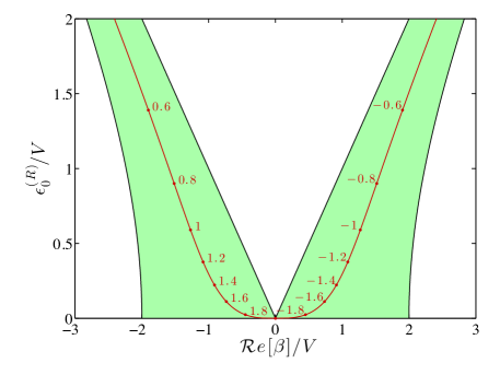
Figure 4: Band structure (green shadowed array) of the model Eq. ($S1$) vs. $\epsilon_{0}^{(R)}$. The red line indicates the trajectory of the defect eigenmode as $\epsilon_{0}^{(R)}$ increases. The red dots and the associated numbers are indicative values of the critical $\epsilon_{0}^{(I)}$ (for the specific $\epsilon_{0}^{(R)}$) above which a defect mode is created.

As $\epsilon_{0}^{(I)}$ increases from zero the propagation constants move into the complex plane. For small values of $\epsilon_{0}^{(I)}$ a perturbative picture is applicable and can explain satisfactorily the evolution of $\beta$’s. Using first order perturbation theory we get that $\beta^{(k)}\approx\beta_{0}^{(k)}+\Gamma_{k,k}$ where $\Gamma_{k,k}\approx-i\epsilon_{0}^{(I)}/(N+1)$. When the matrix elements of the non-Hermitian part of $H$ become comparable with the mean level spacing $\Delta=2V/N$ of the eigenvalues of the Hermitian part $H_{0}$, the perturbation theory breaks down. This happens when $|\epsilon_{cr}^{(I)}|/(N+1)\sim\Delta$ which leads to the estimation $|\epsilon_{cr}^{(I)}|\sim 2V$. In the opposite limit of large $|\epsilon_{0}^{(I)}|$, $H_{0}$ can be treated as a perturbation to $\Gamma$. Due to its specific form, the non-Hermitian matrix $\Gamma$ has only one nonzero eigenvalue and thus, in the large $|\epsilon_{0}^{(I)}|$ limit, there is only one complex propagation constant corresponding to ${\cal R}e\left[\beta_{0}^{(k=(N+1)/2)}\right]=0$, while all other modes will have zero imaginary component (to first order). The above considerations allow us to conclude that for $|\epsilon_{0}^{(I)}|\gg 2V$ a segregation of propagation constants in the complex plane occurs: Below this point all $\beta$’s get an imaginary part which increases in magnitude as $\sim-\epsilon_{0}^{(I)}/N$ while after that only one of them accumulates almost the whole imaginary part $\sim-\epsilon_{0}^{(I)}$ (independent of $N$) and the remaining $N-1$ approaches back to the real axis as $\sim-(2V)^{2}/(N\epsilon_{0}^{(I)})$. This segregation of propagating constants is the analogue of quantum optics Dicke super-radiance transition D54 which was observed also in other frameworks OPR03 ; SZ89 ; C12 ; KSKHSA12 . These predictions are confirmed by our numerical data (see Fig. 4).

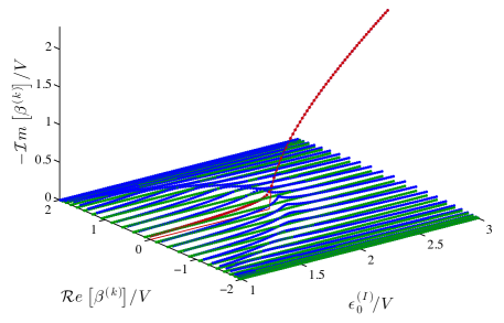
Figure 1: Parametric evolution of the propagation constants $\beta^{(k)}$ of an array of $N=49$ coupled waveguides with one dissipative ($\epsilon_{0}^{(I)}>0$) defect in the middle, as a function of the non-Hermiticity $\epsilon_{0}^{(I)}$ of the defect. The super-radiance point is defined by the condition $\epsilon_{0}^{(I)}=\epsilon_{cr}^{(I)}\equiv+2V$ where the defect mode profile (shown as red dots) switches from non-exponential to exponential decay. Solid red line shows the asymptotic analytical result from Eq. (5). Similar behavior (not shown here) but with the $\beta$’s in the upper complex plane can be observed in the case of gain $\epsilon_{0}^{(I)}<0$ where $\epsilon_{cr}^{(I)}=-2V$.

Delocalization-localization transition and BIC- Next we investigate the structure of the FB modes of the system Eq. (3) in the thermodynamic limit (N$\rightarrow$$\infty$) as $\epsilon_{0}^{(I)}$ crosses the threshold $\epsilon_{cr}^{(I)}$. In the case of real defect, we know that an infinitesimal value of it will lead to the creation of a localized mode (with a real-valued $\beta$ outside of the continuum $[-2V,2V]$ interval) E06 . We want to find out if the same scenario is applicable in the case of imaginary defect. To this end we introduce the ansatz:

$$\phi_{n}=\left\{\begin{array}[]{cc}A^{(+)}\exp(-n\Lambda)&{\rm for}\quad n\geq 0\\ A^{(-)}\exp(n\Lambda)&{\rm for}\quad n\leq 0\end{array}\right.$$ (4)

Continuity requirement of the FB mode at $n=0$ leads to $A^{(+)}=A^{(-)}$. Furthermore, substituting the above ansatz in Eq. (3) for $n=0$ and $n=1$ and after some straightforward algebra we get that

$$\beta=-s\sqrt{4V^{2}-(\epsilon_{0}^{(I)})^{2}}\quad{\rm and}\quad\Lambda=-\ln\left({-\beta-i\epsilon_{0}^{(I)}\over 2V}\right),$$ (5)

where $s\equiv\epsilon_{0}^{(I)}/|\epsilon_{0}^{(I)}|$ denotes the sign of the defect. From Eq. (5) we find that for $|\epsilon_{0}^{(I)}|<|\epsilon_{cr}^{(I)}|\equiv 2V$ the corresponding propagation constant is real while the decay rate is $\Lambda=-i\arctan\left(\epsilon_{0}^{(I)}/\beta\right)$ i.e. a simple phase. In other words the FB modes are extended. In the opposite limit of $|\epsilon_{0}^{(I)}|>|\epsilon_{cr}^{(I)}|$ the propagation constant becomes complex and the corresponding $\Lambda$ takes the form

$$\Lambda=\ln\left({2V\over\left|\epsilon_{0}^{(I)}\right|-\sqrt{(\epsilon_{0}^{(I)})^{2}-4V^{2}}}\right)+i\,s\,{\pi\over 2}$$ (6)

The corresponding inverse localization length is then defined as $\xi^{-1}\equiv{\cal R}e(\Lambda)$ indicating the existence of exponential localization. Therefore we find that a non-Hermitian defect - in contrast to a Hermitian one - induces a localization-delocalization transition at the Dicke super-radiance phase transition points $\epsilon_{cr}^{(I)}=s\times 2V$. We emphasize again that this phase transition and the creation of a localized mode occur for both signs of the non-Hermitian defect and can be induced for both lossy ($\epsilon_{0}^{(I)}>0$) and gain ($\epsilon_{0}^{(I)}<0$) defect.

We have confirmed the theoretical analysis with numerical simulations. In Fig. 2 we report the FB defect mode of our system Eq. (3) for three cases corresponding to (a) $0<\epsilon_{0}<2V$ (below threshold), (b) $\epsilon_{0}=2V$ (at threshold) and (c) $\epsilon_{0}>2V$ (above threshold), and different system sizes. Note that although in the latter case the mode is localized in space, it is not qualified as a BIC since the corresponding propagation constant $\beta$ (see Eq. (5)) is imaginary and therefore the mode is non-stationary. Adding, however, a uniform gain (for lossy defect) $\beta$ or loss (for gain defect) $-\beta$ to the array can turn this state to a BIC with zero imaginary propagation constant. The latter case is experimentally more tractable since adding a global loss will lead to a decay of all other modes while the localized defect mode would be stable having a constant amplitude.

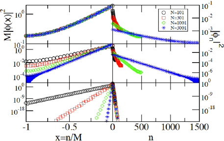
Figure 2: Floquet-Bloch defect mode for various system sizes $N=2M+1$. Left panels report the left part ($n<0$) of these modes (the right part $n>0$ is the same) by employing the scaling $M\phi(x=n/M)$ while the right panels report the right part $n>0$ of these modes without any scaling. In the former representation an extended state is invariant under increase of the size of the system while in the latter, the scale invariance is demonstrated for localized modes. Three defect values of $\epsilon_{0}^{(I)}$ has been used: (upper) Below threshold $0<\epsilon_{0}^{(I)}<2V$ where the mode is delocalized; (middle) At threshold $\epsilon_{0}^{(I)}=2V$ where the mode is critical; (lower) Above threshold $\epsilon_{0}^{(I)}>2V$ where the mode is exponentially localized. Notice that in the case of critical modes (middle panels)

CSC at the phase transition- The existence of the delocalization-localization phase transition posses intriguing questions, one of which is the nature of the FB mode at the transition point associated with $\epsilon_{cr}^{(I)}$. In particular, it is known from the Anderson localization theory, that the eigenfunctions at the metal-to-insulator phase transition are multifractals i.e. display strong fluctuations on all length scales M00 ; FE95 ; W80 . Their structure is quantified by analyzing the dependence of their moments ${\cal I}_{p}$ with the system size $N$:

$${\cal I}_{p}=\frac{\sum_{n}\left|\psi_{n}\right|^{2p}}{(\sum_{n}\left|\psi_{n}\right|^{2})^{2}}\propto N^{-(p-1)D_{p}}.$$ (7)

Above the multifractal dimensions $D_{p}\neq 0$ are different from the dimensionality of the embedded space $d$. Among all moments, the so-called inverse participation number (IPN) ${\cal I}_{2}$ plays the most prominent role. It can be shown that it is roughly equal to the inverse number of non-zero eigenfunction components, and therefore is a widely accepted measure to characterize the extension of a state. We will concentrate our analysis on ${\cal I}_{2}$ of the FB mode at the phase transition point $\epsilon_{cr}^{(I)}$.

We assume that the eigenmodes of Eq. (3) take the following form:

$$\begin{split}\phi_{n}^{(k)}=A^{(-)}e^{iq^{(k)}n}+B^{(-)}e^{-iq^{(k)}n}(n<0)\\ \phi_{n}^{(k)}=A^{(+)}e^{iq^{(k)}n}+B^{(+)}e^{-iq^{(k)}n}(n>0)\\ \end{split}$$ (8)

where $q^{(k)}=q_{r}^{(k)}+iq_{i}^{(k)}$, while the associated propagation constants are in general complex and can be written in the form $\beta^{(k)}\equiv-2V\cos(q^{(k)})=\beta_{r}^{(k)}+i\beta_{i}^{(k)}$. Imposing hard wall boundary conditions to the solutions Eq. (8) i.e. $\phi_{M+1}=\phi_{-M-1}=0$ allow us to express the coefficients $B^{(-)},B^{(+)}$ in terms of $A^{(-)},A^{(+)}$:

$$B^{(\mp)}=-A^{(\mp)}e^{\mp 2iq(M+1)}$$ (9)

At the same time the requirement for continuity of the wavefunction at $n=0$ lead us to the relation

$$A^{(+)}+B^{(+)}=A^{(-)}+B^{(-)}$$ (10)

Substitution of Eqs. (9,10) back into Eq. (3) for $n=0$, lead to a transcendental equation for $q$:

$$V\sin[2(M+1)q]\sin(q)=i\epsilon_{0}^{(I)}\sin^{2}[(M+1)q]$$ (11)

which can be re-written in terms of two equations

$$\sin[(M+1)q]=0;\,\,{\rm or}\,\,\cot[(M+1)q]\sin(q)=i{\epsilon_{0}^{(I)}\over 2V}$$ (12)

We are interested in the structure of the FB mode in the middle of the band corresponding to ${\cal R}e(\beta)=0$. For simplicity of the calculations we assume below that $M+1$ is odd note2 and also remind that the total size of the system is N=2M+1. Imposing the condition ${\cal R}e(\beta)=0$ in the second term of the Eq. (12) we get that $q_{r}=-s\pi/2$ while the imaginary part $q_{i}$ satisfies the following equation

$$s\tanh\bigg{[}(M+1)q_{i}\bigg{]}\cosh(q_{i})=\frac{\epsilon_{0}^{(I)}}{2V}$$ (13)

We will look for a stationary solution at the phase transition point $\epsilon_{0}^{(I)}=s\,2V$ with $\beta_{i}\rightarrow 0$ (or equivalently $q_{i}\rightarrow 0$) in $N\rightarrow\infty$ limit that also satisfies $q_{i}\times(M+1)\sim q_{i}N\rightarrow\infty$ condition. In Eq. (13) we now perform small $q_{i}$ expansion in $\cosh(q_{i})\approx 1+q_{i}^{2}/2$ and large $(M+1)q_{i}$ expansion in $\tanh[(M+1)q_{i}]=\frac{\exp((M+1)q_{i})-\exp(-(M+1)q_{i})}{\exp((M+1)q_{i})+\exp(-(M+1)q_{i})}\approx 1-2\exp(-(N+1)q_{i})\approx 1-q_{i}^{2}/2$. In the large $M$-limit the solution of the last transcendental equation can be found by using the definition of Lambert W-function. We have

$$q_{i}\sim 2\frac{\ln(N+1)}{N+1}.$$ (14)

Substituting back to the expression for the propagation constant we get $\beta=-2V\cos(-s\pi/2+iq_{i})\approx-s\,2V\,iq_{i}$ which in the large $N(M)$-limit results in $\beta=0$. Finally, substituting Eqs. (9,14) back to Eq. (8) we get that the corresponding FB mode takes the form

$$\phi_{n}\propto\exp\left[i(-s\pi/2+iq_{i})|n|\right]=\frac{(-s\,i)^{|n|}}{\left(N+1\right)^{2|n|/(N+1)}}$$ (15)

The FB state described by Eq. (15) is not exponentially localized neither it is extended. It rather falls to an exotic family of critical states and it can quantify better via the IPN ${\cal I}_{2}$. Using Eq. (7) for $p=2$ it is easy to show that the IPN of the FB mode of Eq. (15) is given by Eq. (1). Furthermore, this scaling relation is not consistent with the standard power law Eq. (7) characterizing self-similar (fractal) states. Rather we have an unusual situation of a critical state that it is at the verge of being fractal. To our knowledge such anomalous scaling has been discussed only in completely different context of Hermitian random matrix models ORC11 and were never found to be present in any physical system. Thus our simple set-up constitutes the first paradigmatic system where these CSC can be observed. We have also checked that the critical nature of the defect state is not a consequence of the degenerate band-edge DELA03 being present in the case of the tight-binding system of Eq. (3). This can be achieved by introducing an on-site potential $\epsilon_{n}^{(R)}=\epsilon_{0}^{(R)}(-1)^{n}$ which removes the degeneracy at $\beta=0$. We found that the defect state still exists but its energy ${\cal R}e(\beta)$ is no longer at $0$. It is inside one of two bands and away from all band edges. Amazingly, there is still a critical point (which depends on $\epsilon_{0}^{(R)}$) when the defect state becomes critical and ${\cal I}_{2}\sim\log(N+1)/(N+1)$.

The validity of our analysis has been confirmed by performing detailed numerical calculations. In the inset of Fig. 3 we report using a double-logarithmic plot the scaling of ${\cal I}_{2}$ versus the system size at the phase transition point. A deviation from a straight line (which would be the case of fractal states) is clearly visible as $M$ takes larger values. Instead in the main plot we report the anomalous part of ${\cal I}_{2}$ as a function of $\ln\ln(N+1)$. We see that the data follow a nice straight line, thus confirming the validity of our prediction Eq. (1).

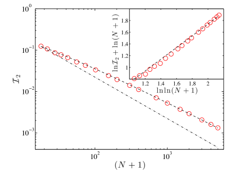
Figure 3: Scaling analysis of the IPN ${\cal I}_{2}$ (see Eq. (7)) of a CSC state versus the system size $N$. In the main panel ${\cal I}_{2}$ (shown as symbols) is plotted versus the size of the system in a double logarithmic plot. Dot-dashed line corresponds to $N^{-1}$ dependence. Dashed line is prediction of Eq. (1) which contains a logarithmic correction. In the inset we plot the same data in a different fashion i.e. $\ln{\cal I}_{2}+\ln(N+1)$ versus $\ln\ln(N+1)$. Straight line with a unit slope confirms the existence of the logarithmic dependence as indicated by our theoretical prediction Eq. (1).

Conclusions - In conclusion we have investigated the structure of non-Hermitian defect states as a function of the defect strength. We have found that these states experienced a phase transition from delocalization to localization as the imaginary part of the refractive index in the defect waveguide approaches a critical value. At the transition point the inverse participation number of this mode scales as $\ln(N)/N$ indicating a weak criticality. This phase transition is accompanied by a mode re-organization which reveals analogies with the Dicke super-radiance. The transition survives periodic pertubations in the refractive index in the waveguide array and the anomalous logarithmic behavior of the inverse participation ratio at the critical point is preserved. It will be interesting to investigate whether this behavior survives in higher dimensions and other type of configurations.

Acknowledgement - We thank A. Ossipov and Y. Fyodorov for useful discussions. This work was sponsored partly by grants NSF ECCS-1128571, DMR-1205223, ECCS-1128542 and DMR-1205307 and by an AFOSR MURI grant FA9550-14-1-0037.

I Supplemental Material

In this section, we show that the critical nature of the defect state is not an artifact of degenerate band-edges appearing in the middle of the band for the tight-binding model of Eqs. (2,3) of the main text. In order to remove the $\beta=0$ degeneracy we introduce a staggering on-site potential as $\epsilon_{n}^{(R)}$=$\epsilon_{0}^{(R)}(-1)^{n}$. Therefore, the new tight-binding equation is:

$$\beta^{(k)}\phi_{n}^{(k)}=-V(\phi_{n+1}^{(k)}+\phi_{n-1}^{(k)})-(\epsilon_{0}^{(R)}(-1)^{n}+\epsilon_{n}^{(I)}\delta_{n0})\phi_{n}^{(k)};\\ S1$$ ()

We propose the following ansatz for odd/even (denoted by superscript o/e) waveguide numbers:

$$\begin{split}\phi_{n}^{(k)(o/e)}=A^{(-)(o/e)}e^{iq^{(k)}n}+B^{(-)(o/e)}e^{-iq^{(k)}n}(n<0)\\ \phi_{n}^{(k)(o/e)}=A^{(+)(o/e)}e^{iq^{(k)}n}+B^{(+)(o/e)}e^{-iq^{(k)}n}(n>0)\\ \end{split} S2$$ ()

In the absence of imaginary defects we get the following dispersion relation:

$$\beta^{(k)}=\pm\sqrt{(\epsilon_{0}^{(R)})^{2}+4V^{2}\cos^{2}q^{(k)}} S3$$ ()

Therefore, the degenerate energy at zero is shifted into the positive or negative branch.

In the presence of defect, and after taking into account the hard wall boundary conditions ($\phi_{M+1}^{(k)(o)}=\phi_{-M-1}^{(k)(o)}=0$) and continuity at n=0, we get two discrete equations for the complex propagation constant $q$:

$$\begin{split}\sin[(M+1)q]=0;\,\,{\rm or}\,\,\,\,\,\,\,\,\,\,\,\,\,\,\,\,\,\,\,\,\,\,\,\,\,\,\,\,\,\,\,\,\,\,\,\,\,\,\,\,\,\,\,\,\,\,\,\,\\ \cot[(M+1)q]\sin(q)=i{\epsilon_{0}^{(I)}\over 2V}.\frac{\epsilon_{0}^{(R)}+\sqrt{(\epsilon_{0}^{(R)})^{2}+4V^{2}\cos^{2}q}}{2V\cos q}\\ \end{split} S4$$ ()

The above equations are consistent with the results presented in the main text at the limit $\epsilon_{0}^{(R)}$$\rightarrow$ 0.

In the localized regime ($|\epsilon_{0}^{(I)}|$$>$ $|\epsilon_{cr}^{(I)}|$), we get $\cot[(M+1)q]\approx i$. By replacing this expression into the second term of Eq. ($S4$), we derive the following cubic relation for $x\equiv\tan q$:

$$\begin{split}2\epsilon_{0}^{(R)}\epsilon_{0}^{(I)}x^{3}+\Big{(}(\epsilon_{0}^{(I)})^{2}-4V^{2}\Big{)}x^{2}+2\epsilon_{0}^{(R)}\epsilon_{0}^{(I)}x+(\epsilon_{0}^{(I)})^{2}=0\end{split} S5$$ ()

The above algebraic equation has three roots. Depending on the value of $\epsilon_{0}^{(I)}$ these roots can be either real or complex. In the former case (i.e. $x$, and therefore $q$, being real) the associated mode is extended, while in the latter one (i.e. $x$, and therefore $q$, being complex) the associated mode is localized. The transition between these types of modes occurs at $\epsilon_{cr}^{(I)}$ and is given as a solution of the following equation:

$$\begin{split}\bigg{(}(4V^{2}-\epsilon_{cr}^{(I)})^{2}\bigg{)}^{3}=\,\,\,\,\,\,\,\,\,\,\,\,\,\,\,\,\,\,\,\,\,\,\,\,\,\,\,\,\,\,\,\,\,\,\,\,\,\,\,\,\,\,\,\,\,\,\,\,\,\,\,\\ 8(\epsilon_{0}^{(R)})^{2}\bigg{(}-2V^{4}+10V^{2}(\epsilon_{cr}^{(I)})^{2}+(\epsilon_{cr}^{(I)})^{4}+2(\epsilon_{cr}^{(I)})^{2}(\epsilon_{0}^{(R)})^{2}\bigg{)}\\ \end{split} S6$$ ()

Furthermore, it can readily be confirmed that, as expected, for $\epsilon_{0}^{(R)}\rightarrow 0$, $\epsilon_{cr}^{(I)}$ approaches to 2.

The associated energy $\beta_{cr}$ of the defect (localized) mode is found after substituting the expression for $\epsilon_{cr}^{(I)}$ from Eq. ($S6$), into Eq. ($S4$). This allows us to evaluate $q^{(cr)}$ which can then be substituted in Eq. ($S3$) in order to get an expression for $\beta_{cr}$.

Next, we investigate the scaling behavior of the defect mode at the transition point $\epsilon_{cr}^{(I)}$. Following the same argumentation as used in the main text, we write $q^{(cr)}$ as $q_{r}^{(cr)}+iq_{i}$, where we assume that $(M+1)q_{i}\rightarrow\infty$ and $q_{i}$ is a small quantity. Substituting back to the transcendental equality of Eq. ($S4$) and expanding each term up to first order in $q_{i}$ we eventually get:

$$q_{i}\sim\frac{\ln(N+1)}{N+1}. S7$$ ()

Considering the fact that ${\cal I}_{2}\sim q_{i}$, it can be deduced that the second moment of the defect mode for the modified model scales anomalously as indicated in Eq. (1) of the main text.

To summarize, we elucidated that the logarithmic scaling of IPR is not a consequence of degenerate band-edge in Anderson model at $\beta=0$.

References

- (1) A. Peres, Quantum Theory: Concepts and Methods, Kluwer Academic Publishers (1993).
- (2) N. F. Mott, Adv. Phys. 16, 49 (1967).
- (3) J. von Neumann and E. Wigner, Z. Phys. 30, 465 (1929).
- (4) Y. Plotnik et al, Phys. Rev. Lett. 107, 183901 (2011).
- (5) S. Weimann et al, Phys. Rev. Lett. 111, 240403 (2013).
- (6) G. Corrielli et al, Phys. Rev. Lett. 111, 220403 (2013).
- (7) C. W. Hsu et al, Nature 499, 188 (2013).
- (8) R. Porter, D. Evans, Wave Motion 43, 29 (2005); C. M. Linton, P. McIver, Wave Motion 45, 16 (2007).
- (9) F. Capasso, et al, Nature358, 565 (1992).
- (10) D. C. Marinica, A. G. Borisov, S. V. Shabanov, Phys. Rev. Lett. 100, 183902 (2008).
- (11) J. Okolowicz, M. Ploszajczak, I. Rotter, Phys. Rep. 374, 271 (2003).
- (12) K. Zhou et al, Opt. Lett. 35, 2928 (2010)
- (13) A. Regensburger et al, Phys. Rev. Lett. 110, 223902 (2013)
- (14) S. Longhi, Bound states in the continuum in -symmetric optical lattices, arXiv:1402.3761 (2014)
- (15) D.N. Christodoulides, F. Lederer, and Y. Silberberg, Nature 424, 817 (2003).
- (16) It is possible to have the same for the defect waveguide (without violating the Kramers-Kronig relations). One way to achieve this is by correcting the changes in the at , due to the presence of , by appropriate adjustment of its width.
- (17) A. Guo, et. al., Phys. Rev. Lett. 103, 093902 (2009).
- (18) T. Eichelkraut et al, Nature Communcations 4, 2533 (2013)
- (19) C. E. Ruter et. al, Nat. Phys. 6, 192 (2010).
- (20) R.H. Dicke, Phys. Rev. 93, 99 (1954).
- (21) V. V. Sokolov, V. G. Zelevinsky, Nucl. Phys. A504, 562 (1989).
- (22) G. L. Celardo et al., J. Phys. Chem. C 116, 22105 (2012); R. Monshouwer et al, J. Phys. Chem. B 101, 7241 (1997).
- (23) J. Keaveney et al, Phys. Rev. Lett. 108, 173601 (2012); M. O. Scully, A. A. Svidzinsky, Science 328, 1239 (2010).
- (24) E. N. Economou, Green’s Functions in Quantum Physics, Springer Series in Solid-State Sciences (Third Edition) (2006).
- (25) A. D. Mirlin, Phys. Rep. 326, 259 (2000); Y. V. Fyodorov and A. D. Mirlin, Int. J. Mod. Phys. 8, 3795 (1994); Y. V. Fyodorov and A. D. Mirlin, Phys. Rev. B 51, 13403 (1995).
- (26) V. I. Falko and K. B. Efetov, Europhys. Lett. 32, 627 (1995); Phys. Rev. B 52, 17413 (1995).
- (27) F. Wegner, Z. Phys. B 36, 209 (1980); H. Aoki, J. Phys. C 16, L205 (1983); M. Schreiber and H. Grussbach, Phys. Rev. Lett. 67, 607 (1991); D. A. Parshin and H. R. Schober, ibid. 83, 4590 (1999); A. Mildenberger, F. Evers, and A. D. Mirlin, Phys. Rev. B 66, 033109 (2002).
- (28) We note that for even there are two critical states that emerge symmetrically around . The rest of the analysis remains qualitatively the same.
- (29) A. Ossipov, I. Rushkin, and E. Cuevas, Journal of Physics: Cond. Matt. 23, 415601 (2011).
- (30) L.I. Deych et al, Phys. Rev. Lett. 91, 096601 (2003)