Shilnikov Homoclinic Bifurcation of Mixed-Mode Oscillations

Abstract

The Koper model is a three-dimensional vector field that was developed to study complex electrochemical oscillations arising in a diffusion process. Koper and Gaspard described paradoxical dynamics in the model: they discovered complicated, chaotic behavior consistent with a homoclinic orbit of Shil’nikov type, but were unable to locate the orbit itself. The Koper model has since served as a prototype to study the emergence of mixed-mode oscillations (MMOs) in slow-fast systems, but only in this paper is the existence of these elusive homoclinic orbits established. They are found first in a larger family that has been used to study singular Hopf bifurcation in multiple time scale systems with two slow variables and one fast variable. A curve of parameters with homoclinic orbits in this larger family is obtained by continuation and shown to cross the submanifold of the Koper system. The strategy used to compute the homoclinic orbits is based upon systematic investigation of intersections of invariant manifolds in this system with multiple time scales. Both canards and folded singularities are multiple time scale phenomena encountered in the analysis. Suitably chosen cross-sections and return maps illustrate the complexity of the resulting MMOs and yield a modified geometric model from the one Shil’nikov used to study spiraling homoclinic bifurcations.

1 Introduction

In 1992, Marc Koper and Pierre Gaspard introduced a three-dimensional model to analyze an electrochemical diffusion problem, in which layer concentrations of electrolytic solutions fluctuate nonlinearly at an electrode [29, 30]. They sought to model mixed-mode oscillations (hereafter MMOs) arising in a wide variety of electrochemical systems. Their analysis revealed a host of complicated dynamics, including windows of period-doubling bifurcations, Hopf bifurcations, and complex Farey sequences of MMO signatures.

They also found regions in the parameter space where the equilibrium point of the system satisfies the Shilnikov condition. Within these regions, they observed that trajectories repeatedly come close to the fixed point, and return maps strongly suggest chaotic motion consistent with a Shilnikov homoclinic bifurcation. However, they were unable to locate a genuine homoclinic orbit to account for this behavior, so it was catalogued as a near homoclinic scenario. In such a scenario, complex and chaotic MMOs could suddenly arise—as if from a homoclinic bifurcation—but without the existence of the homoclinic orbit to serve as an organizing center.

Nevertheless, the Koper model has emerged as a paradigm in studies of slow-fast systems containing MMOs [8, 10]. As its four parameters are varied, local mechanisms such as folded nodes [19, 37] and singular Hopf bifurcation [2, 8, 20, 25, 26] generate small-amplitude oscillations. A global return mechanism allows for repeated reinjection into the regions containing these local objects. The interplay of these local and global mechanisms gives rise to sequences of large and small oscillations characterized by signatures that count the numbers of consecutive small and large oscillations. Shilnikov homoclinic orbits are limits of families of MMOs with an unbounded number of small oscillations in their signatures. When the Shilnikov condition is satisfied, they also guarantee the existence of chaotic invariant sets whose presence in the Belousov-Zhabotinsky reaction was controversial for several years.

The homoclinic orbits that could explain Koper’s original observations have remained elusive. This paper describes their first successful detection. Multiple timescales make numerical study of these homoclinic orbits quite delicate; on the other hand, the presence of slow manifolds allows us to analyze many aspects of the system with low-dimensional maps. We find the homoclinic orbits by exhibiting multiple time scale phenomena such as canards and folded singularities. We first locate such orbits in a five-parameter family of vector fields used to explore the dynamics of singular Hopf bifurcation. After an affine coordinate change, the Koper model is a four-parameter subfamily. Shooting methods that compute trajectories between carefully chosen cross-sections cope with the numerical instability resulting from the singular behavior of the equations. Following identification of a homoclinic orbit in the larger family, a continuation algorithm is used to track a curve on the codimension-one manifold of spiraling homoclinic orbits in parameter space. This manifold intersects the parametric submanifold corresponding to the Koper model, locating the homoclinic orbit that is the target of our search.

This paper is a numerical investigation of the Koper model. The results are not rigorous, so a formal “theorem-proof” style is inappropriate for this discussion. Following the numerical part of the paper, we abstract our reasoning to present a geometric model for the slow-fast decomposition of the homoclinic orbits of the Koper model. This geometric model produces a list of properties that we use to prove the existence of a homoclinic orbit in a slow-fast system. We think these properties may be amenable to verification in the Koper model through the use of interval arithmetic.

2 The Koper model as a slow-fast system

We consider vector fields of the form

$$\varepsilon\dot{x} = f(x,y),$$

(1) $$\dot{y} = g(x,y),$$

where $x\in R^{m}$, $y\in R^{n}$, and the functions $f$ and $g$ are smooth. In this paper, $f$ and $g$ are polynomials. Slow-fast vector fields are those where $\varepsilon\ll 1$. In this case, $x$ is the fast variable and $y$ is the slow-variable.

The Koper model is a frequently studied example and the subject of this paper. It is defined by

$$\varepsilon_{1}\dot{u} = kv-u^{3}+3u-\lambda,$$

(2) $$\dot{v} = u-2v+w,$$

$$\dot{w} = \varepsilon_{2}(v-w),$$

and has two slow variables $v$ and $w$ and one fast variable $u$ when the parameters $\varepsilon_{1}\ll 1$ and $\varepsilon_{2}=1$. The terms $k$ and $\lambda$ are additional parameters. We assume throughout this paper that $\varepsilon_{2}=1$ without further comment.

The study of slow-fast vector fields has advanced rapidly in recent years with specific focus on systems having two slow variables and one fast variable. We recall relevant aspects of the theory that bear on the Koper model. The review paper [10] includes an extensive discussion that provides additional information, especially about mixed mode oscillations.

The set of points defined by $C=\{f=0\}$ in system (2) is called the critical manifold. Fenichel [16] proved the existence of locally invariant slow manifolds near regions of $C$ where $D_{x}f$ is hyperbolic. Trajectories on the slow manifolds are approximated by trajectories of the reduced system on $C$ defined by

(3) $$\dot{y} = g(h(y),y,0),$$

where $h$ is defined implicitly by $f(h(y),y,0)=0$. While the slow manifolds are not unique, compact portions are exponentially close to each other: their distances from each other are $O(\exp(-c/\varepsilon))$ as $\varepsilon\to 0$. We often refer to ‘the’ slow manifold in statements where the choice of slow manifold does not matter. The points $x\in C$ where $D_{x}f$ is singular are called fold points. For the Koper model, $C$ is the zero set of $kv-u^{3}+3u-\lambda$ and the fold curve consists of the points on $C$ with $\frac{3}{k}(u^{2}-1)=0$. The reduced system is given by

(4) $$\frac{3}{k}(u^{2}-1)\dot{u} = u-2v+w,$$

$$\dot{w} = (v-w),$$

where $v=\frac{1}{k}(u^{3}-3u+\lambda)$.

The reduced system is a differential algebraic equation that is the main component of the singular limit of the “full” system (2) as $\varepsilon_{1}\to 0$. The other component of the singular limit comes from the fast part of the full system. The fold curve divides the critical manifold into attracting and repelling sheets where $u^{2}>1$ and $u^{2}<1$ respectively. When trajectories of the full system reach the vicinity of the fold curves, they turn and then flow close to the fast direction to a small neighborhood of the attracting slow manifold. In the singular limit, one has trajectories on the attracting and repelling sheets of the critical manifold that meet at the fold curve separating the sheets. The limiting behavior of the full system from these impasse points is to jump along the fast direction stopping at the first intersection with an attracting sheet of $C$. The addition of fast jumps makes the singular limit a hybrid system whose trajectories (called candidates) consist of concatenations of slow segments that solve the reduced system and fast jumps parallel to the fast direction. As we describe below, fast jumps may occur at points of $C$ which are not fold points.

Rescaling time of the reduced system produces a desingularized reduced system that extends to the fold curve. In the case of the Koper model, the desingularized reduced system is

(5) $$\dot{u} = u-2v+w,$$

$$\dot{w} = \frac{3}{k}(u^{2}-1)(v-w),$$

where $v=\frac{1}{k}(u^{3}-3u+\lambda)$. Discrete time jumps of trajectories that reach the fold curve of (5) are added to the reduced model to reflect the limiting behavior of the full system. However, there are exceptional trajectories of the full system that flow from an attracting slow manifold to a repelling slow manifold without making a jump at the fold curve. The singular limits of these trajectories flow to equilibrium points of (5) which lie on its fold curves. Since the time rescaling of desingularization reverses the direction of time on the repelling sheet of $C$ where $u^{2}<1$, we follow trajectories of (5) backwards in time “through” the singularity. At any location along such a backward trajectory, a jump to one of the attracting sheets of the slow manifold is allowed along the fast direction. This makes the reduced system multi-valued and hence still more complicated. See [7] for further discussion of this construction of a hybrid reduced model in the context of the forced van der Pol system.

The desingularized reduced system of a fast-slow system can have two types of equilibrium points. Equilibria of the “full” system are retained as equilibria of the desingularized reduced system. Additionally, points on a fold curve may become equilibria of the desingularized reduced system because the time rescaling factor vanishes at these points. For the Koper model, these folded singularities are solutions of the equations $kv-u^{3}+3u-\lambda$, $u-2v+w=0$ and $u^{2}-1=0$. (The third of these equations replaces the equation $\dot{z}=0$ for an actual equilibrium.) The folded singularities are further classified as folded nodes, saddles, saddle-nodes, and foci depending on their type as equilibria of the desingularized reduced system. The folded singularities mark transitions along the fold curve where the trajectories of the reduced system (without desingularization) approach the fold curve or flow away from it. They are also close to places where the full system might have trajectories that contain segments on an attracting slow manifold that proceed to follow the repelling slow manifold without an intervening jump. Trajectory segments that flow for time $O(1)$ in the slow time scale along a repelling slow manifold of a slow-fast systems are called canards. They have been the subject of intense study since they were found in periodic orbits of the forced van der Pol equation [4, 12]. They also play an important role in the dynamics of the Koper model and are part of the homoclinic orbits we find. See Figure 1.

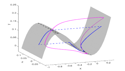
(a)

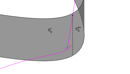
(b)

Fig. 1: (a) Shilnikov homoclinic orbit (magenta curve) found in the Koper model, defined by (6), alongside a typical singular homoclinic orbit defined by trajectories (blue solid curves) lying on the critical manifold (gray surface) of the system, concatenated with instantaneous jumps (blue dashed curves) to different branches of the critical manifold. Fold lines are given by black dashed curves. Section 7 discusses families of singular homoclinic orbits in detail. (b) A cartoon of the local dynamics. The homoclinic orbit departs along the two-dimensional unstable manifold of the equilibrium and returns by passing very close to a folded singularity of the singular system, given by the black dot on the fold line separating the sheets $S^{r}_{0}$ and $S^{a+}_{0}$ of the critical manifold. These sheets perturb to attracting and repelling slow manifolds for small values of the singular perturbation parameter $\varepsilon$.

The dynamics of the full system close to folded singularities is significantly more complicated than suggested by the reduced system. Benoit [3] observed that trajectories of the full system near folded nodes of the reduced system can make small amplitude oscillations in directions that involve both fast and slow variables. The oscillations are manifest in twisting of the attracting and repelling slow manifolds, as visualized by Desroches [10]. The maximum number of small oscillations of trajectories passing through this region is bounded, with a bound determined from a normal form for the folded node [3, 37]. In the Koper model and other slow-fast systems, small oscillations associated with folded nodes together with “global returns” produce mixed mode oscillations [10].

Our goal in this paper is to locate a homoclinic orbit of the Koper model when its equilibrium is a saddle-focus. The initial portion of such an orbit consists of small amplitude oscillations as the homoclinic orbit spirals away from the equilibrium along its unstable manifold (see Fig. 1). In single time scale systems, both shooting and boundary value methods can be used to find the homoclinic orbit. With both types of algorithms, as well as in theoretical analysis of the dynamics near the homoclinic orbit, trajectories are decomposed into a local portion in a neighborhood of the equilibrium and a global portion that lies outside that neighborhood. Linearization or higher order approximations are used to identify the local stable and unstable manifolds, and then numerical methods are used to find the global return.

Because the homoclinic bifurcation is a codimension one phenomenon, an “active” parameter is used in locating the bifurcation. Extending the phase space to include the active parameter, the homoclinic orbit becomes a transverse intersection of the families of stable and unstable manifolds of the curve of equilibria in the extended system. Shooting methods locate the global return by computing a two parameter family of initial value problems whose initial conditions depend upon the active parameter and a coordinate that parameterizes trajectories in the unstable manifold. The intersections of these trajectories with a cross-section of the local stable manifolds forms a surface while the family of local stable manifolds intersects the cross-section in a curve. The cross-section is three dimensional in the extended phase space, so the intersections of the stable and unstable manifolds can cross transversally.

Straightforward implementation of this strategy fails in the Koper model, as Koper discovered in his original investigation. The slow-fast structure of the problem makes portions of the global return trajectories so sensitive that continuous dependence upon initial conditions appears to fail for numerical solutions of initial value problems. This apparent discontinuity of trajectories has been documented in the “canard explosions” of the van der Pol equation with constant forcing [21]. The crux of our analysis of the Koper homoclinic model is to decompose the global returns into segments, each of which can be reliably computed with either forward or backward integration. This strategy has worked with other examples like the canard explosion [24] of the van der Pol system with constant forcing, and it proves successful again here.

When the Koper model equilibrium is a saddle-focus, its two dimensional unstable manifold is a source of small amplitude oscillations. The number of small amplitude oscillations is unbounded as trajectories leave the equilibrium. However, their magnitude changes quickly unless the ratio of the real and complex parts of the complex eigenvalues at the equilibrium is small. Parameter regions close to a Hopf bifurcation yield small ratios, so choosing parameters in such a region is part of our strategy for finding homoclinic orbits. Hopf bifurcation in slow-fast systems takes several forms that depend upon whether the two dimensional subspace of center directions lie in fast directions, slow directions, or a mixture of the two. The third case is called singular Hopf bifurcation, and it is the case that occurs in the Koper model. In systems with two slow variables, singular Hopf bifurcation is closely associated with a phenomenon in the desingularized reduced system called folded saddle-node, type II (FSNII)[37]. This occurs in the desingularized reduced system when an equilibrium (that is not a folded singularity) crosses a fold curve as a parameter is varied. As the equilibrium crosses the fold curve, a folded singularity passes through the same point, and its type switches between a fold node and a folded saddle. Singular Hopf bifurcations are found at a distance $O(\varepsilon)$ from the FSNII point.

The dynamics of a model system with an FSNII bifurcation have been analyzed by Guckenheimer and Meerkamp [25]. The model they studied is obtained by truncating a Taylor expansion at the FSNII bifurcation: it can be viewed informally as a normal form for this problem and for singular Hopf bifurcation. Moreover, this normal form is closely related to the Koper model. With the addition of a single cubic term and an appropriate affine coordinate change, it contains the Koper system as a subfamily. We make use of this relationship below, first finding a homoclinic orbit of the larger family and then continuing it to parameters that lie in the (transformed) Koper family. The FSNII normal form has many different types of bifurcations and small amplitude chaotic behavior is possible [25]. Complicated small scale dynamics of this system raise the possibility of homoclinic orbits that are more complicated than the ones we exhibit in this paper.

A key aspect of the FSNII dynamics relevant to our search for homoclinic orbits in the Koper model is the intersection of the unstable manifold of the equilibrium with the repelling slow manifold. Since both of these manifolds are two dimensional, we expect them to intersect along isolated trajectories. The homoclinic orbits we find contain segments close to such intersections. As trajectories in the unstable manifold emerge from the equilibrium point, they may follow the repelling slow manifold for some distance, producing a canard that can then jump away from the repelling manifold. Part of our computational task is to identify the jump point that yields the homoclinic orbit.

By definition, the homoclinic orbit contains a branch of the stable manifold of the equilibrium. We find that this branch lies close to the attracting slow manifold for a substantial distance. A second key part of our computations stems from the observation that the stable manifold of the equilibrium crosses the attracting slow manifold as a parameter is varied and that the homoclinic bifurcation lies exponentially close to this parameter value. Finding this crossing is delicate because the stable manifold passes through a region where extensions of the normally hyperbolic attracting manifold twist. Most of the studies of mixed mode oscillations of the Koper model to date are based upon local analysis of oscillations close to perturbations of a folded node or near the equilibrium. Here, we need to study trajectories that interact with both the equilibrium and a twisting, attracting slow manifold, a situation that remains poorly understood. Our homoclinic orbit lies close to such trajectories, and further analysis of their dynamics is likely to produce interesting results.

We close this section with three remarks:

1. Folded singularities are defined for the reduced system that is the singular limit of a slow-fast system. In the full system with time scale parameter $\varepsilon>0$, these entities are no longer defined. However, it is useful to identify points that are located where their influence is manifest. We use the term twist region to describe sets in the phase space of the full system where an (extended) attracting slow manifold twists around a canard. Numerically, we locate approximations to these points as folded nodes of the reduced system obtained by setting $\varepsilon=0$.

2. We consider only parameter values of the Koper model for which its equilibrium point $p_{eq}$ has a pair of complex conjugate eigenvalues $\rho\pm i\omega$ and one real eigenvalue $\lambda$ with $\lambda<0<\rho$. This constraint forces the equilibrium to be within a distance $O(\varepsilon)$ of the folded singularity of the singular limit. This requirement is explained further in Section 3 below. When we study the singular limit of the system, we do so along parameter curves along which the equilbrium remains a saddle-focus.

3. Numerical studies of slow-fast systems always rely upon particular choices of the time scale parameter $\varepsilon>0$, while the theory focuses upon dynamics that is present for “small enough $\varepsilon$.” It is rare that one can verify that a particular choice of $\varepsilon$ is indeed small enough to fall within the scope of particular theorems. Nonetheless, the theory provides a guide to expected behavior in the numerics, explaining observations that would otherwise appear anomalous. These studies are based upon the presumption that $\varepsilon$ is sufficiently small and test this presumption by examining the dynamics for different values of $\varepsilon$. However, like the theory, the problem of connecting the behavior observed at specific values of $\varepsilon>0$ with the singular limit is nontrivial. Our approach here is to show that we find behavior consistent with that described by perturbations from the singular limit.

3 The singular Hopf extension of the Koper model

We now introduce a family of vector fields with two slow variables and one fast variable that contains a singular Hopf bifurcation [2, 8, 20, 25, 26]. It is given by

$$\varepsilon\dot{x} = y-x^{3}-x^{2},$$

(6) $$\dot{y} = z-x,$$

$$\dot{z} = -\nu-ax-by-cz,$$

where $\varepsilon,\nu,a,b,$ and $c$ are parameters, $x$ is the fast variable, and $y$ and $z$ are the slow variables. We denote $\alpha=(\varepsilon,\nu,a,b,c)$ and define $P$ to be the five dimensional space of parameters $\alpha$. The critical manifold is the $S$-shaped cubic surface $\{y=x^{3}+x^{2}\}$ with two fold lines at $L_{0}$ defined as $\{x=0\}$ and $L_{-2/3}$ defined as $\{x=-2/3\}$. In our numerical investigations, we set $\varepsilon=0.01$ unless otherwise noted.

“The” slow manifold $S$ has sheets $S^{a-}_{\varepsilon}$, $S^{r}_{\varepsilon}$ and $S^{a+}_{\varepsilon}$ that lie close to the sheets of the critical manifold $C$ defined by $C\cap\{x<-2/3\}$, $C\cap\{-2/3<x<0\}$ and $C\cap\{0<x\}$. Away from the fold lines, forward trajectories are attracted to $S^{a\pm}_{\varepsilon}$ and repelled from $S^{r}_{\varepsilon}$ at fast exponential rates (see for eg. [27] for a derivation of estimates using the Fenichel normal form).

After the affine coordinate change defined by $(x,y,z)=((u-1)/3,(kv-\lambda+2)/27,2v-w-1)/3)$ [10], scaling time by $-k/9$ and the substitutions

$$(\varepsilon,a,b,c,\nu)=(-k\varepsilon_{1}/81,18/k,81\varepsilon_{2}/k^{2},-9(\varepsilon_{2}+2)/k,(3\lambda-6-3k)\varepsilon_{2}/k^{2}),$$

the Koper model becomes a parametric subfamily of (6), with parameters satisfying the equation

(7) $$2b+a(a+c)=0.$$

Note that the above parametric equation corrects a sign error in Desroches et al.[10]. We work henceforth with the Koper model in the form given by (6).

The corresponding desingularized slow flow of the system (6) is given by

$$\dot{x} = z-x$$

(8) $$\dot{z} = -(2x+3x^{2})(\nu+ax+b(x^{2}+x^{3})+cx).$$

In analogy to (5), this two-dimensional system is derived by rescaling time with the term $(2x+3x^{2})$. The origin is always an equilibrium of (8), so $n=(0,0,0)\in L_{0}$ is a folded singularity of (6).

We consider only parameter sets of (6) satisfying the following conditions: (i) the reduced system (8) has a singularity at $(0,0)$, which is a folded node for $\nu>0$, (ii) exactly one equilibrium point $p_{eq}$ exists in the full system with $\nu=O(\varepsilon)$, with a pair of complex conjugate eigenvalues $\rho\pm i\omega$ and one real eigenvalue $\lambda$, (iii) the stable manifold $W^{s}$ of $p_{eq}$ is one-dimensional and the unstable manifold $W^{u}$ of $p_{eq}$ is two-dimensional ($\lambda<0<\rho$). Our notation for $W^{s}$ and $W^{u}$ hides their dependence on the parameter values.

We comment on requirements (i) and (ii) above. When studying the singular limit $\varepsilon\to 0$ of system (6), condition (ii) requires that $\nu$ must also change, so that the limiting system has a folded saddle-node, type II.

In this regime, small-amplitude oscillations may be due to intersections of the attracting and repelling slow manifolds as they twist around each other near a folded singularity [10, 37] or to the spiraling of trajectories near the unstable manifold of the equilibrium or both. We find that the homoclinic orbits we seek pass through the twisting region, so that the interactions of $W^{s}$ and $W^{u}$ with the slow manifolds of the system play a significant role in their existence. In particular, the homoclinic orbits we locate contain segments that lie close to the intersection of $W^{u}$ with the repelling slow manifold $S^{r}_{\varepsilon}$, similar to the homoclinic orbits that form the traveling wave profiles for the FitzHugh-Nagumo equation [23], a system with one slow variable and two fast variables. The homoclinic orbits also contain segments where $W^{s}$ lies close to $S^{a+}_{\varepsilon}$.

To focus upon trajectories that pass through a twist region before encountering the equilibrium, we use the position of the equilibrium as an alternative to the parameter $\nu$. This position is given by $p_{eq}=(x_{eq},x_{eq}^{2}+x_{xeq}^{3},x_{eq})$, so $\nu=-x_{eq}[a+bx_{eq}(x_{eq}+1)+c]$ and the family can be parameterized by $(x_{eq},a,b,c)$ instead of $(\nu,a,b,c)$. With this new parameterization, the equilibrium point remains fixed as the parameters $a$, $b$, and $c$ are varied, while the twist region is a small neighborhood of the origin. In the rest of this paper, we set $x_{eq}=-0.03$ whenever we study system (6) with $\varepsilon>0$, except in the concluding remarks where we let the distance between $p_{eq}$ and $L_{0}$ vary with $\varepsilon$.

4 The shooting procedure

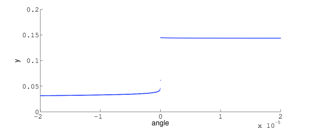
Fig. 2: Height ($y$ value) of forward trajectories in $W^{u}$ crossing the surface $\{x=-0.05\}$ as a function of angle. An angle of 0 corresponds to a trajectory of height $y=0.1$ lying in $S^{r}_{\varepsilon}\cap W^{u}$. The parameter set is $(\varepsilon,a,b,c)\approx(0.01,-4.416165,2.891404,5.725663)$.

The boundary value algorithm HOMCONT [15] was created within the package AUTO [13] to compute homoclinic orbits with a collocation procedure. Nonetheless, we have been unsuccessful in using AUTO or MATCONT [11] to locate a Shilnikov homoclinic orbit in (6) when $\varepsilon\ll 1$. The stiffness of the vector field appears to prevent convergence to a homoclinic solution even when very large numbers of collocation points are used. Shooting algorithms are also problematic since trajectories of $W^{u}$ diverge rapidly from each other near a canard segment of the homoclinic orbit. Thus, parameterizing trajectories in $W^{u}$ by an angular variable and varying the angle of an initial point is not well-suited to locating a Shilnikov homoclinic orbit because trajectories in $W^{u}$ are extremely sensitive to the angle of an initial condition near $p_{eq}$ (see Fig. 2). This issue suggests a different shooting strategy than varying this angle. Instead, we define an angular variable, $\theta$ that parametrizes trajectories in $W^{u}$ smoothly (including as a function of the parameters) and regard it as an additional parameter for the system. So $W^{u}=\cup_{\theta}W^{u}_{\theta}$. The shooting procedure can then fix $\theta$ and use another parameter in the search for a homoclinic orbit that contains $W^{u}_{\theta}$.

Our extended family has the six dimensional parameter space $\bar{P}$ with coordinates $(\alpha,\theta)$. The homoclinic submanifold of the extended parameter space persists as a codimension-one object [22]. To obtain defining equations $\psi:\bar{P}\to\Sigma$ for this manifold, we choose the surface of section $\Sigma$ defined by $z=0$, set $s^{\alpha}$ to be the first intersection (in backward time) of $W^{s}$ with $\Sigma$, $u^{\alpha}_{\theta}$ to be the first intersection (in forward time) with decreasing $z$ of $W^{u}_{\theta}$ with $\Sigma$ and $\psi(\alpha,\theta)=s^{\alpha}-u^{\alpha}_{\theta}$. The relation $\psi(\alpha,\theta)=0$ defines a four dimensional submanifold $\bar{H}$ of $\bar{P}$. The projection of $\bar{H}$ to $P$ is a homoclinic manifold $H$ consisting of parameters for which (6) has a homoclinic orbit.

Approximations to ${s}^{\alpha}$ and ${u}^{\alpha}_{\theta}$ are obtained by numerically integrating trajectories with initial conditions in the linear stable and unstable subspaces of $p_{eq}$. Denoting these approximations by $\tilde{s}^{\alpha}$ and $\tilde{u}^{\alpha}_{\theta}$, the formula $\tilde{\psi}(\alpha,\theta)=\tilde{s}^{\alpha}-\tilde{u}^{\alpha}_{0}$ approximates the defining equations. Previous studies [5, 6, 34, 35] analyze the convergence of the solutions $\tilde{\alpha}$ of $\tilde{\psi}=0$ as the distance of the initial conditions to $p_{eq}$ tends to $0$. Hyperbolicity of the fixed point, which is satisfied by $p_{eq}$, is required for these estimates.

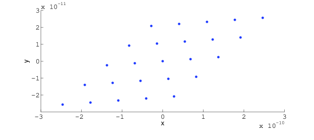
Fig. 3: The image of a square grid of parameters $(a,b)$ under the shooting function $\psi_{\Sigma_{0}}$ in the surface $\Sigma_{0}=\{z=0\}$. The location of the Shilnikov homoclinic orbit is found to be close to the parameters $\tilde{\alpha}\approx(0.01,-0.03,-0.2515348,-1.6508230,1)$. Integrations were performed for a square grid of points $(a,b)$ in the domain of $\psi_{\Sigma_{0}}$, specified by $a\in[\tilde{a}-2*10^{-6},\tilde{a}+2*10^{-6}]$ and $b\in[\tilde{b}-2*10^{-6},\tilde{b}+2*10^{-6}]$.

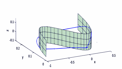
(a)

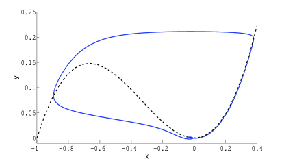
(b)

Fig. 4: Homoclinic orbit (blue curve) to $p_{eq}$ specified by the parameters $\theta=0$ and $\tilde{\alpha}$ in Fig. 3. The critical manifold $C=\{y=x^{2}+x^{3}\}$ is given by the light green manifold in (a) and its $xy$-projection is given by the black dashed curve in (b).

We now reduce the number of active parameters by fixing $\varepsilon=0.01$, $\theta=0$, $c=1$, and $x_{eq}=-0.03$. Note that our choice of $\Sigma$ as the hyperplane $z=0$ is motivated by the complicated dependence of $W^{s}$ on the parameters [19]. This section slices through a twist region and is close enough to the equilibrium point that small changes in $\alpha$ do not produce large jumps in $s^{\alpha}$. These choices leave $a$ and $b$ as active parameters to vary in $\bar{P}$ to locate an approximate homoclinic orbit by solving the approximate defining equations $\tilde{\psi}=0$.

Fig. 3 illustrates the regularity of the defining equations $\tilde{\psi}=0$ on a small rectangle $A\subset R^{2}$ of points in the space of active parameters $(a,b)$. Blue dots represent the images of a $5\times 5$ lattice of points in $A$ under the shooting function $\tilde{\psi}$. The data indicate that $\tilde{\psi}$ is close to affine and regular on $A$ and that its image contains the point $(0,0)$, implying that there exists $(\tilde{a},\tilde{b})\in A$ with $\tilde{\psi}(\tilde{\alpha})=0$, where $\tilde{\alpha}$ is the parameter set with second and third components given by $(\tilde{a},\tilde{b})$. This in turn implies the existence of a Shilnikov homoclinic orbit, depicted by the blue curve in figure 4.

5 Continuation of the homoclinic orbit

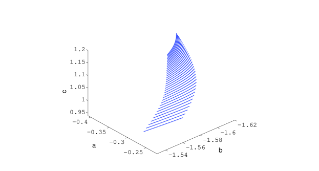
Fig. 5: A portion of $H$ created with continuation. The portion was projected from $(\theta,a,b,c)$ space to $(a,b,c)$ space. The apparent curves show the results of continuation in the direction of one of the two nullvectors of $J=D\xi$.

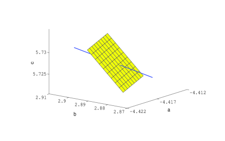
(a)

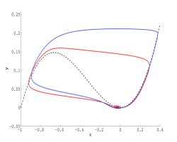
(b)

Fig. 6: (a) Continuation of a curve (blue) on $H_{0}^{\prime}$ through a local patch of the Koper manifold (yellow) defined by Eq. 7. (b) A comparison of the homoclinic orbit defined by the parameter set $\tilde{\alpha}$ (blue curve) and the homoclinic orbit lying in the Koper subfamily (red curve) obtained via the continuation in (a), with parameter set $\beta=(\varepsilon_{\beta},a_{\beta},b_{\beta},c_{\beta})\approx(0.01,-4.416165,2.891404,5.725663)$. The eigenvalues of $p_{eq}$ for the Koper homoclinic are $(\rho\pm i\omega,\lambda)\approx(0.790204\pm 8.482321i,-1.576071)$, so $p_{eq}$ satisfies the Shilnikov condition.

Continuation algorithms [32] are widely used to find curves of bifurcations in multi-dimensional parameter spaces. Here, the goal is to find an intersection of the homoclinic manifold $H$ with the subfamily of (6) that yields the Koper model. The tangent space to $\bar{H}$ is the null space of $D\psi$. We estimate $D\psi$ with a central finite difference method to provide starting data for continuation calculation of curves on $\bar{H}$. These are iterative calculations that use a predictor-corrector algorithm to compute a sequence of parameter values $\alpha_{j}$ on $H$:

1. Prediction step: Compute $w^{0}=\alpha^{j}+hv^{j}$, where $v^{j}\in{\rm~{}null}(D\psi)$ and $h$ is our chosen stepsize.

2. Correction step: Choose a tolerance $\delta$ and iteratively compute
   $w^{k+1}=w^{k}-(D\psi)^{+}(w^{k})\psi(w^{k})$, where $J^{+}$ is the Moore-Penrose pseudoinverse matrix of $J$ defined by $J^{+}=J^{T}(JJ^{T})^{-1}$.

3. Stopping criterion: Stop when $||w^{k+1}-w^{k}||<\delta$ and let $\alpha^{j+1}=w^{k+1}$.

We fix $\varepsilon=0.01$, $x_{eq}=-0.03$ and $\theta$, and then use $c$ as the third active parameter in addition to $a$ and $b$ in the continuation calculation of a curve on $H$. Fig. 5 shows a computation of a patch of $H$ in $(a,b,c)$ space with different curves corresponding to different values of $\theta$. Fig. (6a) shows a transversal intersection of one of these curves on $H$ with the Koper manifold given by Eq. 7. The affine transformations relating (6) to the Koper model will rescale and shift the homoclinic orbit (shown in Fig. (6b)) while preserving its topological structure.

6 Transversality of invariant manifolds

The homoclinic orbit exists for the full system (6) when a trajectory in the two dimensional unstable manifold $W^{u}$ flows along $S^{r}_{\varepsilon}$ to a point where it jumps to $S^{a-}_{\varepsilon}$, then flows along $S^{a-}_{\varepsilon}$ to its fold, jumps again to $S^{a+}_{\varepsilon}$, then flows along this manifold to the folded node region where it connects to the one dimensional local stable manifold $W^{s}$ of the equilibrium. This only happens when the parameter values lie in the homoclinic submanifold $H$ of the parameter space. We can visualize how this happens by looking at intersections of $W^{s}$ and $W^{u}$ in the cross-section $z=0$ that pass through the twist region. On this cross-section, $W^{s}$ sweeps out a curve $C$ and $S^{a}_{\varepsilon}$ sweeps out a two-dimensional surface $S$ as the parameter $a$ is varied. Fig. (7) shows this intersection in $(x,y,n)$ space where the local coordinate $n$ is defined via $(x,y,a)\cdot\eta=n$ and $\eta$ is a unit vector normal to a small patch of $S$. This choice of coordinates increases the angle of intersection that occurs in $(x,y,a)$ space. As $a$ varies, the surface swept out by $W^{u}$ intersects the curve swept out by $W^{s}$ transversally, demonstrating that the solution of the defining equation for the homoclinic orbit is regular.

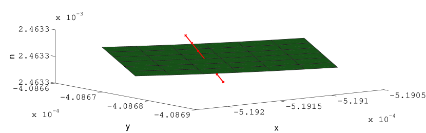
Fig. 7: Transversal intersection in $\{z=0\}$ of surface $S$ (green) swept out by $S^{a}_{\varepsilon}$ and curve $C$ (red) swept out by $W^{s}$ as the parameter $a$ is varied. Intersection corresponds to homoclinic orbit defined by $\beta$ as given in Fig. 6. Integrations were performed for $a\in[a_{\beta}-3*10^{-5},a_{\beta}+3*10^{-5}]$.

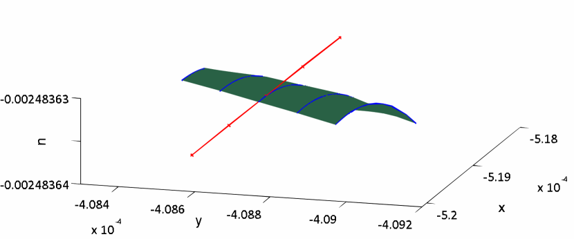
Fig. 8: Transversal intersection in $\{z=0\}$ of the surface $S^{\prime}$ (green) swept out by $S^{r}_{\varepsilon}\cap W^{u}$ and the curve $C$ (red) swept out by $W^{s}$ as the parameter $a$ is varied. The intersection corresponds to the homoclinic orbit defined by $\beta$ as given in Fig. 6. Integrations were performed for five equally spaced values of $a\in[a_{\beta}-3*10^{-5},a_{\beta}+3*10^{-5}]$. Intersections of $W^{u}$ (blue curves) for different values of $a$ are shown.

It is difficult to directly compute the relevant portion of $W^{u}$ since it contains canards. The two-dimensional subset of $S^{r}_{\varepsilon}$ we want to compute consists of trajectories which leave the fixed point $p_{eq}$ along its unstable manifold and follow the repelling slow manifold $S^{r}_{\varepsilon}$ up to some height $y$, before finally jumping across to $S^{a-}_{\varepsilon}$. In order to locate this part of $S^{r}_{\varepsilon}$, we first integrate backwards a line of initial conditions at a particular height lying midway between the jump from $S^{r}_{\varepsilon}$ to $S^{a+}_{\varepsilon}$. These backward trajectories jump to $S^{r}_{\varepsilon}$ and flow along it before turning along one of the two branches of $W^{s}$ as they approach the equilibrium point. Since trajectories lying in $W^{u}$ separate those trajectories which follow the two branches of $W^{s}$, we can locate the trajectory $\gamma$ in $S^{r}_{\varepsilon}\cap W^{u}$ with a bisection method. We then compute an approximation to the strong unstable manifold of $\gamma$ by integrating forward points on either side of $W^{u}$ that lie close to $\gamma$. This strategy relies on the fact that trajectories in $W^{u}$ approximate leaves of the strong unstable foliation of $S_{r}$ for the canard trajectory in $S^{r}_{\varepsilon}\cap W^{u}$. As discussed in Sec. 4, the resulting heights of the trajectories are extremely sensitive to the angle as illustrated in Fig. (2). Since the calculation of $W^{u}$ is lengthy and indirect, we located the homoclinic orbit parameters by instead finding intersections of $W^{s}$ with $S^{a+}_{\varepsilon}$. Fig. (7) shows that as we vary the parameter $a$, the intersections of $W^{s}$ with $S^{a+}_{\varepsilon}$ are similar to those of $W^{u}$ and $W^{s}$ shown in Fig. ((8)). As before, this figure locates the transversal intersections of $W^{u}$ and $W^{s}$ on the surface of section specified by $\{z=0\}$. Trajectories lying on $S^{r}_{\varepsilon}\cap W^{u}$ sweep out a two-dimensional surface $S^{\prime}$ and the stable manifold sweeps out a curve $C$. The objects $S^{\prime}$ and $C$ intersect transversally (Fig. 8).

7 Singular homoclinic orbits

As $\varepsilon\to 0$, trajectories for (6) have singular limits consisting of concatenations of fast segments (“jumps”) parallel to the $x$-axis and segments that are trajectories of the reduced system on the critical manifold. Transitions from slow to fast segments in the singular limit trajectories can occur at folds or anywhere along a slow segment on the repelling sheet of the critical manifold. The slow trajectory segments are contained in invariant manifolds that are approximated by invariant manifolds appearing in the singular limit $\varepsilon\to 0$ of the system. These invariant manifolds provide a substrate for our theoretical analysis of the homoclinic orbits in Section 9.

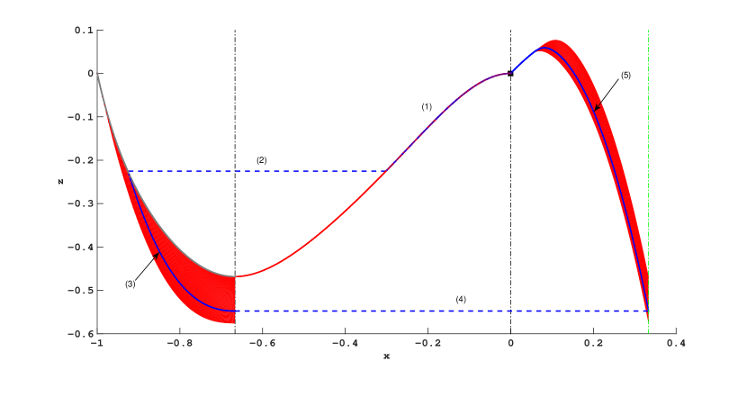
Fig. 9: Nonunique singular cycles of the desingularized reduced system (8). Recall that stability is reversed on $S^{r}_{0}$, the region $-2/3<x<0$, because of the time reparametrization used to desingularize the reduced system. A typical cycle in this family contains trajectories on $C$ (blue solid curves) and jumps (blue dashed curves): (1) a segment of the unstable manifold of the folded saddle-node (0,0), (2) a jump to $S^{a-}_{0}$, (3) a segment of a trajectory flowing forward on $S^{a-}_{0}$ to the left jump curve at $x=-2/3$, (4) a jump to $S^{a+}_{0}$ ending on the green dashed line $\{x=1/3\}$, (5) a trajectory segment on $S^{a+}_{0}$ connecting the end of this jump to the folded node at (0,0). The slow segments of all the singular homoclinic orbits lie in the red regions. Parameter set is $(\nu,a,b,c)=(0,a_{\beta},b_{\beta},c_{\beta})$, where subscripted parameters are defined in Fig. 6.

When $\varepsilon>0$, the unstable manifold $W^{u}$ and the repelling slow manifold $S^{r}_{\varepsilon}$ are each two dimensional, so they can intersect transversally along a trajectory. Moreover, $W^{u}$ contains segments aligned with the unstable foliation of $S^{r}_{\varepsilon}$ beginning where its trajectories jump from $S^{r}_{\varepsilon}$. Tiny variations in initial conditions on $W^{u}$ yield trajectories that turn abruptly at different heights, as illustrated in Fig. (2). This fast portion of $W^{u}$ turns again to follow $S^{a-}_{\varepsilon}$ exponentially closely, then jumps to $S^{a+}_{\varepsilon}$ and follows this manifold to the twist region. The singular limits of these transitions are given by smooth one dimensional maps whose composition with one another maps a segment of $W^{u}$ to a section of $S^{a+}_{0}$ that passes through the folded node.

We are interested in studying the singular limit of a system for which the equilibrium point is a saddle-focus that remains $\varepsilon$-close to the folded singularity. These conditions can be satisfied only when the distance from the equilibrium point to the fold scales with $\varepsilon$: in the system (6), this implies $\nu=O(\varepsilon)$. In particular, when $\nu=\varepsilon=0$ the origin is an equilibrium point of the full system that is a folded saddle-node, type II. Summarizing, the singular limit of the homoclinic orbits can be decomposed as follows:

• An initial segment which lies in $W^{u}$ within the repelling sheet $S^{r}_{0}$ of the critical manifold.

• A jump from $S^{r}_{0}$ to the attracting sheet $S^{a-}_{0}$ of the critical manifold.

• A slow trajectory on $S^{a-}_{0}$ that ends at the fold at $x=-2/3$.

• A jump from the fold of $S^{a-}_{0}$ to $S^{a+}_{0}$

• A slow trajectory that follows $S^{a+}_{0}$ back to the saddle-node equilibrium at the origin.

We reemphasize here that slow trajectories are defined for the reduced system (8) at an FSN II bifurcation.

The saddle-node point of this system has a single unstable separatrix and a two dimensional stable manifold with boundary. This creates a lack of uniqueness in the singular limit as shown in Fig. (9). In the reduced system, trajectories that jump from the unstable manifold to $S^{a-}_{0}$ continue to the fold curve $x=-2/3$ where they jump to points lying in the stable manifold of the saddle-node. Jumps from the unstable manifold of the saddle-node that occur anywhere on $S^{r}_{0}$ yield trajectories that return to the saddle-node. However, when $\varepsilon>0$, the geometry near the equilibrium becomes much more complicated. The equilibrium has a one dimensional stable manifold, and this manifold intersects the attracting slow manifold $S^{a+}_{\varepsilon}$ only for parameters lying in a codimension one manifold of the parameter space. Moreover, $S^{a+}_{\varepsilon}$ may twist around the stable manifold near the location of a folded-node in the reduced system. Section 9 investigates the persistence of each of the transitions between segments of the singular homoclinic orbit as $\varepsilon$ becomes positive. Establishing persistence requires transversality hypotheses that are formulated there.

8 Geometry and returns of the twist region

We now turn to a study of the return map to a suitably chosen cross-section near the Shilnikov homoclinic orbit we have found. The classical analysis of Shilnikov begins with a homoclinic orbit of a three dimensional vector field that has a very special form. First, it is assumed that the vector field is linear in a neighborhood $U$ of an equilibrium $p$ and that the eigenvalues $\lambda,\rho\pm i\omega$ at $p$ satisfy $|\rho/\lambda|<1$. Cross-sections $\Sigma_{1}$ and $\Sigma_{2}$ are chosen in $U$, and the flow map from $\Sigma_{1}$ to $\Sigma_{2}$ is computed explicitly. The second assumption is that the “global return” from $\Sigma_{2}$ back to $\Sigma_{1}$ is an affine map. The return map obtained by composing these two flow maps is then proved to have hyperbolic invariant sets. Since hyperbolic invariant sets persist under perturbation of the vector field, homoclinic orbits of vector fields that do not have this special form still have nearby hyperbolic invariant sets. In particular, the Shilnikov analysis applies to the homoclinic orbits of (6) with the parameter set $\beta$ (as in Fig. 6). However, we expect that two aspects of the slow-fast structure of (6) may significantly distort the “standard” Shilnikov return map: (1) the twist region may introduce additional twisting of the flow near the homoclinic orbit, and (2) the strong attraction and repulsion to the slow manifolds might make the global return map from $\Sigma_{2}$ to $\Sigma_{1}$ almost singular. We investigate these issues, producing modifications of the Shilnikov return map suitable for the homoclinic orbits we have located in (6).

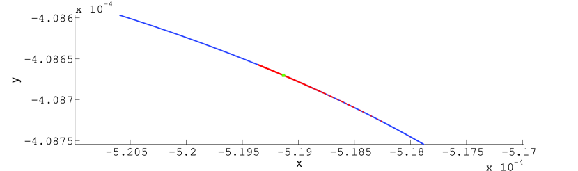
Fig. 10: A segment of $S^{a+}_{\varepsilon}$ on $\{z=0\}$ (blue curve) and its first return (red points). The first intersection of $W^{s}$ with $\{z=0\}$ is depicted by the green square. Parameter set is $\beta$.

We consider the parameter set $\beta$ (as in Fig. 6) and analyze the returns of a thin strip $\Sigma$ near $S^{a+}_{\varepsilon}\cap\{z=0\}$. Exponential contraction of the flow onto $S^{a+}_{\varepsilon}$ suggests that $\Sigma$ may be mapped into itself in the vicinity of its intersection with the homoclinic orbit. Numerical computations suggest that this does happen (Fig. (10)). Approximating $\Sigma$ by a small segment $I$ parametrized by the $x$-coordinate, the corresponding one-dimensional approximation to the return map $R:I\to I$ reveals complicated dynamics (Fig. (11a)). In particular, we find a sequence of fixed points in steep portions of the map $R$ that accumulate at the homoclinic orbit intersection. This agrees with previous analyses of homoclinic orbits to spiraling equilibrium points that identified a countable number of periodic orbits of decreasing Hausdorff distance to the Shilnikov homoclinic orbit [17, 36]. The novel behavior here is that these fixed points lie in steep portions of the return map whose trajectories contain canard segments (Fig. (11b)). These periodic orbits may have a few additional twists (small-amplitude oscillations) associated with reinjection into the twist region, in addition to the spiraling local to the equilibrium point.

An issue of concern is whether the twisting inside twist regions significantly distorts the return map. We explore this issue by comparing the geometry we find in the twist region with what is known about the twisting of slow manifolds in twist regions. In order to make this comparison, we must briefly revisit the slow flow equations.

In studies of the folded node normal form, Benoit [3] and Wechselberger [37] relate the ratio of eigenvalues $\mu=w_{1}/w_{2}$ of the folded node in the reduced system to the number of intersections of the (extended) attracting and repelling slow manifolds. The number $j$ of intersections is estimated by the formula $j=1+[(\mu-1)/2]$, and this also estimates the maximal number of small oscillations of trajectories passing through the twist region in the full system. As further elucidated by Krupa and Wechselberger [31], this estimate breaks down when the folded node is too close to a folded saddle-node. Here, the folded node is too close because $\nu=O(\varepsilon)$ while the results of Krupa and Wechselberger [31] require that $\nu=O(\varepsilon^{1/2})$ or larger. Nonetheless, we use the value of $\mu$ as a guide for our numerical investigations.

In the present instance, the folded node of our reduced system equations (8) has eigenvalues $w_{1}\approx-0.920102$ and $w_{2}\approx-0.0798982$ at the parameter set $\beta$. Thus we estimate $j=1+[(11.5159-1)/2]=6$. However, since the equilibrium point lies in the intersection of the extended slow manifolds, $S^{r}_{\varepsilon}$ has an infinite number of turns that yield a countable number of intersections with $S^{a}_{\varepsilon}$ (Fig. (12)). Although the twist region serves to strongly contract volumes of the phase space, the equilibrium point produces the large numbers of small-amplitude oscillations. It seems that the twisting inside the twist region does not contribute significantly to the geometry of the return map near the homoclinic orbit.

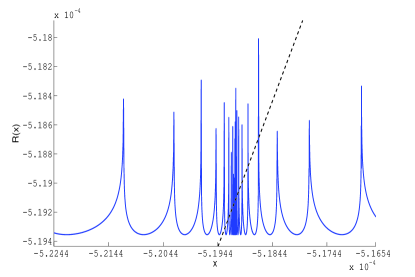
(a)

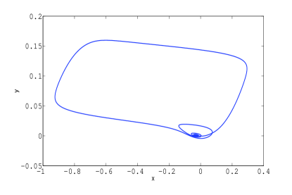
(b)

Fig. 11: (a) The return map $R$ of points in $I$, where both $(x,y)\in I$ and $R(x,y)\in R(I)$ are parametrized by their $x$-coordinates. Points $(x,R(x))$ lie on the solid blue curve, and the fixed points that also lie on the line $x=R(x)$ (dotted black) belong to periodic orbits that intersect the cross section $z=0$ just once. (b) Periodic orbit corresponding to the fixed point $p\approx-5.18996*10^{-4}$ of the map $R$. Parameter set is $\beta$.

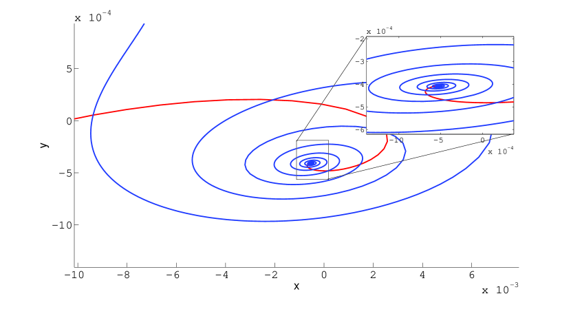
Fig. 12: Intersection of the extensions of $S^{a}_{\varepsilon}$ (red) and $S^{r}_{\varepsilon}$ (blue) in the section $\{z=0\}$. Inset shows magnification of spiraling of $S^{r}_{\varepsilon}$ near the first intersection of $W^{s}$ with $\{z=0\}$. Parameter set is $\beta$.

Since trajectories beginning in $I$ have canard segments when $I$ intersects $S^{r}_{\varepsilon}$, we examine the resulting distortion by focusing on a section closer to the equilibrium point. Fig. (13) shows not only that $I$ intersects $S^{r}_{\varepsilon}$ countably many times near to the equilibrium point, but also that canard lengths of forward trajectories are organized smoothly in neighborhoods of $S^{r}_{\varepsilon}$. The property of countable intersections is explained by the “local” Shilnikov map (in reverse time) applied to initial points in $S^{r}_{\varepsilon}$. Backwards trajectories flowing past the equilibrium point spiral very close to $W^{s}$ by the time the trajectory exits a neighborhood of the equilibrium. The distribution of canard segment lengths implies that the return map of $I$ stretches and folds subsets depending on how the subsets straddle the spiral of the repelling slow manifold.

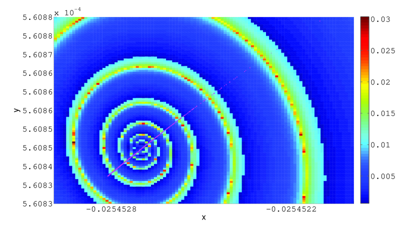
Fig. 13: Intersection of $I$ (purple) with $S^{r}_{\varepsilon}$ in the cross-section $\{z=-0.025\}$. Color values denote heights ($y$-values) attained by trajectories beginning in a $100\times 100$ grid of initial conditions $(x,y,-0.025)$, where $x\in[-0.025453,-0.025452]$ and $y\in[5.6083*10^{-4},5.6088*10^{-4}]$. Stopping conditions are $x=-2/3$ and $y=x^{2}+x^{3}\pm 0.004$. Heights computed from projection of trajectory endpoint onto the critical manifold $\{y=x^{2}+x^{3}\}$. Parameter set is $\beta$.

We get additional insight into the return map using arguments that resemble the Exchange Lemma [28]. This result analyzes the Jacobian of a flow map for trajectories that jump from a slow manifold of saddle type along its unstable manifold. Consider the two dimensional system

$$\varepsilon\dot{x} = 1$$

$$\dot{y} = \lambda y.$$

The flow map of this system from the section $x=0$ to the section $y=1$ is given by $x(1)=\frac{-1}{\lambda}\log y(0)$, with derivative $\left(\frac{-1}{\lambda y(0)}\right)=\frac{-1}{\lambda}\exp(-\lambda x(1))$. Note that this derivative grows exponentially with the distance a trajectory flows along the slow repelling manifold. For us, this is a source of stretching in the global return map of the system (6). We consider trajectories in $W^{u}$ near $S^{r}_{\varepsilon}$ that jump to $S^{a-}_{\varepsilon}$. The arrival points of these curves can be projected onto $S^{a-}_{\varepsilon}$ along its strong stable foliation. So long as this projection is transverse to the trajectories on $S^{a-}_{\varepsilon}$, the stretching that comes from the varying jump points on $S^{r}_{\varepsilon}$ is maintained. Similarly, jumps from $S^{a-}_{\varepsilon}$ to $S^{a+}_{\varepsilon}$, projected onto $S^{a+}_{\varepsilon}$ along its strong stable foliation, sweep out a curve on $S^{a+}_{\varepsilon}$. If this curve is transverse to the flow on $S^{a+}_{\varepsilon}$, the stretching in the global return is once again maintained.

Of course, there is also fast contraction to the attracting manifolds as well. Unless contraction of the flow along $S^{a+}_{\varepsilon}$ in the folded node region dominates the stretching originating along $S^{r}_{\varepsilon}$, we can expect that the global return map to be approximately a rank one map of large norm for the trajectories that have longer canards. This is apparent in the spikes of Figure 11.

We now verify the claim that stretching is maintained in the global return map. Fix two compact, planar cross-sections $\Sigma_{0}$ and $\Sigma_{1}$, transverse to $W^{u}$ and $W^{s}$, respectively. The global return map $R:\Sigma_{0}\to\Sigma_{0}$ can then be decomposed into the two maps $\varphi:\Sigma_{0}\to\Sigma_{1}$ and $\psi:\Sigma_{1}\to\Sigma_{0}$, so that $R=\psi\circ\varphi$. Points beginning in $\Sigma_{1}$ make small oscillations around $W^{s}$ before spiraling out along $W^{u}$ and hitting $\Sigma_{0}$. Later, we give an analytical approximation of the local map $\psi$.

We compute $D\varphi(p)$ with central differences, where $p$ is a $10^{-10}$ perturbation of the point where the homoclinic orbit intersects $\Sigma_{0}$. The matrix $D\varphi(p)$ has singular values $\sigma_{1}\approx 1.53064$ and $\sigma_{2}\approx 2.66223*10^{-7}$, indicating that the global part of $R$ is close to rank one due to strong contraction onto the attracting slow manifolds.

The Jacobian $D\psi$ of the local part of the return map is approximated analytically. First, transform coordinates with the real Jordan form $P^{-1}JP=J^{\prime}$, where $J$ is the Jacobian of (6) at $p_{eq}$. We denote transformations of variables $x$, maps $\zeta$, and subsets $\Sigma$ by primes $x^{\prime}$, $\zeta^{\prime}$, and $\Sigma^{\prime}$. Thus, the unstable subspace of $p_{eq}$ becomes parallel to the $x^{\prime}y^{\prime}$-plane and the stable subspace becomes parallel to the $z^{\prime}$-axis. Following Shilnikov, $\psi^{\prime}:\Sigma_{1}^{\prime}\to\Sigma_{0}^{\prime}$ and its derivative $D\psi^{\prime}$ are approximated explicitly from the normal form of the spiraling equilibrium point:

(9) $$\psi^{\prime}(x^{\prime},y^{\prime}) = (re^{\rho\theta/\omega},de^{-\lambda\theta/\omega}),$$

where $r=\sqrt{x^{\prime 2}+y^{\prime 2}}$, $\tan\theta=y^{\prime}/x^{\prime}$, and $d$ is a small, fixed height of $\Sigma_{1}^{\prime}$ above $(0,0,0)$.

We recover the Jacobian $D\psi$ by transforming $D\psi^{\prime}$ to the original coordinates on the cross-sections $\Sigma_{0,1}$. By the chain rule, we have $DR(p)=D\psi(\varphi(p))\circ D\varphi(p)$, with eigenvalue magnitudes $|\lambda_{1}|\approx 80166$ and $|\lambda_{2}|\approx 2*10^{-16}$. We have not tried to confirm the relative accuracy of the small eigenvalue, but clearly it is very small. Note also that the stretching factor in the local map can be shown to become unbounded by picking points approaching the stable manifold on $\Sigma_{1}$ and a sequence of cross-sections $\Sigma_{0}$ with decreasing heights. These points spiral out along the unstable manifold. The number $m$ of turns that the trajectory makes before intersecting $\Sigma_{0}$ determines the appropriate solution of the multivalued function $\theta=\arctan(y^{\prime}/x^{\prime})+2m\pi$ in (9). The effect on the resulting Jacobian matrix $D\psi^{\prime}$ is multiplication by a diagonal matrix with entries $e^{2m\pi\rho/\omega}$ and $e^{-2m\pi\lambda/\omega}$,both of which are larger than $1$.

9 A geometric model of Shilnikov homoclinic orbits

This section abstracts our analysis of the Shilnikov homoclinic orbit in the Koper model with a list of geometric conditions that are sufficient to prove the existence of such homoclinic orbits in slow-fast systems. In the context of this geometric model, the previous sections can be regarded, retrospectively, as numerical evidence that these conditions are satisfied along a particular curve of parameter values parametrized by $\varepsilon$ in the Koper model.

The geometric model is formulated in terms of a three dimensional slow-fast vector field $X_{\varepsilon}$ with two slow and one fast variable that depends upon additional parameters.

Our first hypothesis is that the reduced system $X_{0}$ (without desingularization) has singular cycles like those shown in Fig. 9:

Singular Cycles Hypothesis:

• The reduced vector field $X_{0}$ has an $S$-shaped critical manifold with sheets $S^{a-}$, $S^{r}$ and $S^{a+}$ separated by fold curves $L^{-}$ and $L^{+}$. $S^{a-}$and $S^{a+}$ are attracting while $S^{r}$ is repelling. The folds are generic.

• $X_{0}$ has a folded saddle-node $p_{eq}$. This point lies on a curve of equilibrium points for the full system $X_{\varepsilon}$ that are saddle-foci for $\varepsilon>0$.

• Beginning at $p_{eq}$, the singular cycles consist of

  1. a segment of the unstable manifold $W^{u}$ lying entirely in $S^{r}$,

  2. a jump from $W^{u}$ to $S^{a-}$,

  3. a segment that flows along $S^{a-}$ to $L^{-}$,

  4. a jump from $L^{-}$ to $S^{a+}$,

  5. a segment that flows along $S^{a+}$ back to $p_{eq}$.

• Following jumps from $L^{-}$ to $S^{a+}$, all of the points of $S^{a+}$ from candidates following the first four steps of this process form a curve $K$ lying in the basin of attraction of $p_{eq}$.

Remark: In the Koper model and other slow-fast systems with an FSNII bifurcation, the equilibrium point is a focal saddle only when it is $O(\varepsilon)$ distant from the FSNII point. Thus the second item in this list of hypothesis implies that the distance from the equilibrium to the twist region of the system scales with $\varepsilon$. System (6) satisfies this scaling hypothesis along a curve obtained by setting $\nu=\varepsilon\bar{\nu}$ and using $\bar{\nu}$ as a parameter which is fixed when letting $\varepsilon\to 0$.

Proving the persistence of the singular cycles requires additional hypotheses that are expressed in terms of transversality. We continue to refer to the repelling and attracting slow manifolds that perturb from the sheets $S^{r}$ and $S^{a\pm}$ for $\varepsilon>0$ as $S^{r}_{\varepsilon}$ and $S^{a\pm}_{\varepsilon}$.

Transversality Hypotheses:

• In the singular limit, the image of the jump curve from $W^{u}$ to $S^{a-}$ is transverse to the vector field of the reduced system.

• Similarly, the curve $K$ defined above is transverse to the vector field of the reduced system on $S^{a+}$.

• For $\varepsilon>0$ small, the unstable manifold of the equilibrium point $p_{eq}$ intersects the repelling slow manifold $S^{r}_{\varepsilon}$ transversally in a trajectory $\gamma_{\varepsilon}$.

• In the four-dimensional extended phase space that includes a parameter $\lambda$, the stable manifolds of $p_{eq}$ sweep out a two-dimensional surface as $\lambda$ is varied. This surface intersects the three-dimensional attracting slow manifold transversally along a trajectory $\beta_{\varepsilon}$. For each $\varepsilon>0$, $\beta_{\varepsilon}$ only exists for a particular parameter value $\lambda=\lambda_{h}(\varepsilon)$.

• The trajectories $\beta_{\varepsilon}$ have a limit as $\varepsilon\to 0$. This limit intersects the curve $K$ defined above.

Remark: The last item on this list of hypotheses has not been investigated thoroughly. Systems with an FSNII bifurcation can be rescaled so that the system has a regular limit as $\varepsilon\to 0$ [20, 25]. We think that the intersections of $W^{s}$ and $S^{a+}_{\varepsilon}$ that we have analyzed in this paper scale nicely with variations of $\varepsilon$ when the remaining parameters are suitably scaled, but have little evidence to substantiate this presumption. The small amplitude dynamics associated with FSNII bifurcations have not yet been studied systematically.

We now state our main theorem about the geometric model:

Theorem 1.

Let $X_{\varepsilon}$ be a slow-fast vector field with two slow variables and one fast variable that depends upon an additional parameter $\lambda$. If $X_{0}$ satisfies the singular cycle hypothesis, and if $X_{\varepsilon}$ satisfies the tranversality hypotheses, then there is an $\varepsilon_{0}>0$ so that for each $0<\varepsilon<\varepsilon_{0}$, there is a value of $\lambda=\lambda(\varepsilon)$ for which $X_{\varepsilon}$ has a homoclinic orbit.

Outline of proof: Define a cross-section $\Sigma_{J}$ orthogonal to the fast direction in the middle of jumps from $L^{-}$ to $S^{a+}$. Denote by $L^{J}$ the curve on $\Sigma_{J}$ that projects onto $L^{-}$ along the fast direction. Since homoclinic orbits are formed by branches of the stable manifold of $p_{eq}$, we prove the theorem by starting at $p_{eq}$ and following its stable manifold $W^{s}$ backward in time. There are intervals of $\lambda$ near $\lambda_{h}(\varepsilon)$ for which the jump points of $W^{s}$ from $S^{a+}_{\varepsilon}$ cross $K$. The fast segments of these jumps intersect $\Sigma_{J}$ in a smooth curve $A$. Projection of $A$ to $S^{a+}_{\varepsilon}$ along its fast foliation gives a curve that is close to a trajectory of the reduced system on $S^{a+}$. The second transversality hypothesis implies that $L^{J}$ and $A$ are transverse.

Now return to $p_{eq}$ and follow trajectories of its unstable manifold $W^{u}$ until they jump to $S^{a+}_{\varepsilon}$. An exponentially thin wedge of angles in $W^{u}$ gives trajectories that follow $S^{r}_{\varepsilon}$ for varying distances, jumping to $S^{a-}_{\varepsilon}$ along strong unstable manifolds of $S^{r}_{\varepsilon}$. These trajectories turn to follow $S^{a-}_{\varepsilon}$ where trajectories are approximated by trajectories of the reduced system. The first transversality hypothesis implies that the width of this strip of trajectories, measured orthogonal to the flow direction, will be $O(1)$. When the strip reaches the vicinity of $L^{-}$, it jumps to $S^{a+}_{\varepsilon}$, intersecting $\Sigma_{J}$ in a curve $L^{J}_{\varepsilon}$. By a classical result of Levinson [33], $L^{J}_{\varepsilon}$ is $C^{1}$ close to $L^{J}$. Consequently, when $\varepsilon>0$ is small enough, $L^{J}_{\varepsilon}$ and $A$ intersect transversally in $\Sigma_{J}$ close to a point of $\Sigma_{J}$ lying on a singular cycle. The point $L^{J}_{\varepsilon}\cap A$ lies on the homoclinic orbit, and the theorem is proved.

In addition to proving the existence of the homoclinic orbit, we want to use the arguments in Section 8 to analyze its return map and prove that there are chaotic invariant sets nearby. Moreover, these invariant sets contain MMOs with unbounded numbers of small amplitude oscillations in their signatures:

Theorem 2.

Let $X_{\varepsilon}$ be a slow-fast vector field with two slow and one fast variable that depends upon an additional parameter $\lambda$. Assume that (1) $X_{0}$ satisfies the singular cycle hypothesis, (2) $X_{\varepsilon}$ satisfies the tranversality hypotheses and (3) that the equilibrium $p_{eq}$ satisfies the Shilnikov condition $-\rho/\mu<1$ for its eigenvalues $\rho\pm i\omega$ and $\mu$ when $\varepsilon>0$. Then, there are chaotic invariant sets in any neighborhood of the homoclinic orbit of $X_{\varepsilon}$. These invariant sets include an infinite number of periodic orbits that make a single global return around the homoclinic orbit. The number of small amplitude oscillations in this set of periodic mixed mode oscillations is unbounded.

Outline of proof: Let $\Sigma_{fn}$ be a cross-section to $X_{\varepsilon}$ in its folded-node region. We establish that its return map resembles Figure 11. Due to the strong contraction along $S^{a+}_{\varepsilon}$, this return map will be close to rank one with image aligned along $I=S^{a+}_{\varepsilon}\cap\Sigma_{fn}$. We study the returns of a thin strip $\bar{I}$ around $I\subset\Sigma_{fn}$ to $\Sigma_{fn}$. The intersection $\xi$ of the stable manifold of $p_{eq}$ with $\Sigma_{fn}$ never returns. Shilnikov’s original analysis [36] of the local flow map establishes (1) that points that approach $\xi$ make increasing numbers of small amplitude oscillations along $W^{u}$ before flowing along $S^{r}_{\varepsilon}$, and (2) the Jacobian of the flow map has a direction with strong expansion. The arguments presented already in Section 8 shows that this expanding direction becomes aligned with the vector field on $S^{r}_{\varepsilon}$ as trajectories jump from $S^{r}_{\varepsilon}$ to $S^{a-}_{\varepsilon}$. Arriving at $S^{a-}_{\varepsilon}$, our transversality hypotheses imply that the expanding direction retains a component transverse to the slow flow on $S^{a-}_{\varepsilon}$. The transversality hypotheses also imply that expansion transverse to the slow flow on $S^{a+}_{\varepsilon}$ is preserved following the jump from $S^{a-}_{\varepsilon}$ to $S^{a+}_{\varepsilon}$. When flowing along $S^{a+}_{\varepsilon}$, strong contraction compresses the image of $\bar{I}$ into an exponentially thin neighborhood of $S^{a+}_{\varepsilon}$. Thus when points of $\bar{I}$ return to $\Sigma_{fn}$, their Jacobian is nearly rank one but (by (2) above) with strong expansion along $I$.

As in Figure 11, the spiral formed as $\bar{I}$ flows past $p_{eq}$ returns to $\Sigma_{fn}$ with monotone branches that cut through $\bar{I}$. Each of these branches contains a fixed point at the intersection of a periodic MMO with $\Sigma_{fn}$, and the returns that remain within a fixed set of $n$ branches constitute hyperbolic invariant sets on which the return map is conjugate to the shift map on sequences of $n$ symbols.

10 Concluding Remark

We have given a fairly complete description of a Shilnikov homoclinic orbit in the Koper model, and we have formulated abstract hypotheses that imply it occurs in a structurally stable bifurcation for sufficiently small $\varepsilon_{1}$. Our numerical investigations suggest that these hypotheses are satisfied.

The Koper model is only moderately stiff in the regime we investigated, raising the question as to whether the qualitative structure of the homoclinic orbits remains unchanged as one approaches the singular limit of the system. In response to this question, we performed a continuation of the singular Hopf normal form homoclinic orbit in Fig. (6) along a parametric path satisfying $\nu=\varepsilon\bar{\nu}$ with $\bar{\nu}$ fixed. On such a path, the distance from the saddle focus to the FSNII scales with $\varepsilon$. As $\varepsilon$ decreases from $0.01$ to approximately $0.003$, the resulting picture agrees with our analysis of the reduced system (Eq. (8)): the Shilnikov orbits become better approximated by concatenations of slow trajectories on $C$ with jumps across branches of $C$.

References

- [1] E. Allgower and K. Georg, Numerical Continuation Methods: An Introduction, Springer-Verlag, New York, 1990.
- [2] S. M. Baer and T. Erneux, Singular Hopf bifurcation to relaxation oscillations, SIAM Journal on Applied Mathematics, 46 (1986), pp. pp. 721–739.
- [3] E. Benoît, Canards et enlacements, Institut des Hautes Études Scientifiques. Publications Mathématiques, 72(1990), pp. 63–91.
- [4] É Benoît , J.-L. Callot, F. Diener, and M. Diener, Chasse au canards, Collect. Math., 31:37–119, 1981.
- [5] W.-J. Beyn, Global bifurcations and their numerical computation, in Continuation and Bifurcations: Numerical Techniques and Applications, D. Roose et. al., ed., vol. 313 of NATO ASI Series, Springer Netherlands, 1990, pp. 169–181.
- [6] , The numerical computation of connecting orbits in dynamical systems, IMA J. Num. Anal., 10 (1990), pp. 379–405.
- [7] K. Bold, C. Edwards, J. Guckenheimer, S. Guharay, K. Hoffman, J. Hubbard, R. Oliva, and W. Weckesser. The forced van der Pol equation. II. Canards in the reduced system. SIAM J. Appl. Dyn. Syst., 2(4):570–608 (electronic), 2003.
- [8] B. Braaksma, Singular Hopf bifurcation in systems with fast and slow variables, Journal of Nonlinear Science, 8 (1998), pp. 457–490.
- [9] M. Brøns, M. Krupa, and M. Wechselberger, Mixed mode oscillations due to the generalized canard phenomenon, Fields Institute Communications, 49:39–63, 2006.
- [10] M. Desroches, J. Guckenheimer, B. Krauskopf, C. Kuehn, H. Osinga, and M. Wechselberger, Mixed-mode oscillations with multiple time scales, SIAM Review, 54 (2012), pp. 211–288.
- [11] A. Dhooge, W. Govaerts, and Yu. A. Kuznetsov, MATCONT: A MATLAB package for numerical bifurcation analysis of ODEs, ACM Trans. Math. Software, 29 (2003), pp. 141–164. Available online from \urlhttp:// www.matcont.ugent.be/.
- [12] M. Diener, The canard unchained or how fast/slow dynamical systems bifurcate, The Mathematical Intelligencer, 6:38–48, 1984.
- [13] E. Doedel, AUTO: Software for continuation and bifurcation problems in ordinary differential equations. Available online from \urlhttp://indy.cs.concordia.ca/auto/.
- [14] F. Dumortier and R. Roussarie, Canard cycles and center manifolds, Mem. Amer. Math. Soc., 121 (1996), pp. 457–490.
- [15] Champneys, A. R. and Kuznetsov, Yu. A. and Sandstede, B., A numerical toolbox for homoclinic bifurcation analysis, Internat. J. Bifur. Chaos Appl. Sci. Engrg., 6 (1996), pp. 867–887.
- [16] N. Fenichel, Persistence and smoothness of invariant manifolds for flows, Indiana Univ. Math. J., 21 (1972), pp. 193–226.
- [17] P. Glendinning and C. Sparrow, Local and global behavior near homoclinic orbits, J. Stat. Phys., 35 (1984), pp. 645–696.
- [18] A. Goryachev, P. Strizhak, and R. Kapral, Slow manifold structure and the emergence of mixed-mode oscillations, J. Chem. Phys., 107(18):2881–2889, 1997.
- [19] J. Guckenheimer, Return maps of folded nodes and folded saddle-nodes, Chaos, 18 (2008).
- [20] , Singular Hopf bifurcation in systems with two slow variables, SIAM Journal on Applied Dynamical Systems, 7 (2008), pp. 1355–1377.
- [21] J. Guckenheimer, K. Hoffman and W. Weckesser, Numerical computation of canards, Int. J. Bif. Chaos 10 (2000), pp. 2669–87
- [22] J. Guckenheimer and P. Holmes, Nonlinear Oscillations, Dynamical Systems, and Bifurcations of Vector Fields, Springer-Verlag, Berlin, New York, 1983.
- [23] J. Guckenheimer and C. Kuehn, Computing slow manifolds of saddle-type, SIAM J. Appl. Dyn. Syst., 8(3):854–879, 2009.
- [24] J. Guckenheimer and D. LaMar, Periodic orbit continuation in multiple time scale systems, Numerical continuation methods for dynamical systems, pp. 253–267, Underst. Complex Syst., Springer, Dordrecht, 2007.
- [25] J. Guckenheimer and P. Meerkamp, Unfoldings of singular Hopf bifurcation, SIAM Journal on Applied Dynamical Systems, 11 (2012), pp. 1325–1359.
- [26] J. Guckenheimer and H. M. Osinga, The singular limit of a Hopf bifurcation, DCDS-A, 32 (2012), pp. 2805 – 2823.
- [27] C.K.R.T. Jones, Geometric singular perturbation theory, vol. 1609 of Lec. Notes in Math., Springer Berlin Heidelberg, 1995.
- [28] C.K.R.T. Jones and N. Kopell, Tracking invariant manifolds with differential forms in singularly perturbed systems,, J. Differential Equations, 108 (1994), pp. 64–88.
- [29] M. T. M. Koper and P. Gaspard, Mixed-mode and chaotic oscillations in a simple model of an electrochemical oscillator, J. Phys. Chem., 95 (1991), pp. 4945–4947.
- [30] , The modeling of mixed-mode and chaotic oscillations in electrochemical systems, J. Chem. Phys., 96 (1992), pp. 7797–7813.
- [31] M. Krupa and M. Wechselberger, Local analysis near a folded saddle-node singularity. J. Differential Equations 248 (2010), no. 12, 2841–2888.
- [32] Y. Kuznetsov, Elements of Applied Bifurcation Theory, Springer-Verlag, New York, 1998.
- [33] N. Levinson, Perturbations of discontinuous solutions of non-linear systems of differential equations. Acta Math., 82 (1950), 71-106.
- [34] X.-B. Lin, Using Melnikov’s method to solve Silnikov’s problems, Proc. R. Soc. Edinburgh A, 116 (1990), pp. 295–325.
- [35] S. Schecter, Rate of convergence of numerical approximations to homoclinic bifurcation points, IMA J. Num. Anal., 15 (1995), pp. 23–60.
- [36] L.P. Šilnikov, A case of the existence of a denumerable set of periodic motions, Sov. Math. Dokl., 6 (1965), pp. 163–166.
- [37] M. Wechselberger, Existence and bifurcation of canards in in the case of a folded node, SIAM Journal on Applied Dynamical Systems, 4 (2005), pp. 101–139.