Age, size, and position of H ii regions in the Galaxy

Abstract

Aims. This work aims at improving the current understanding of the interaction between H ii regions and turbulent molecular clouds. We propose a new method to determine the age of a large sample of OB associations by investigating the development of their associated H ii regions in the surrounding turbulent medium.

Methods. Using analytical solutions, one-dimensional (1D), and three-dimensional (3D) simulations, we constrained the expansion of the ionized bubble depending on the turbulent level of the parent molecular cloud. A grid of 1D simulations was then computed in order to build isochrone curves for H ii regions in a pressure-size diagram. This grid of models allowed to date large sample of OB associations and was used on the H ii Region Discovery Survey (HRDS).

Results. Analytical solutions and numerical simulations showed that the expansion of H ii regions is slowed down by the turbulence up to the point where the pressure of the ionized gas is in a quasi-equilibrium with the turbulent ram pressure. Based on this result, we built a grid of 1D models of the expansion of H ii regions in a profile based on Larson laws. The 3D turbulence is taken into account by an effective 1D temperature profile. The ages estimated by the isochrones of this grid agree well with literature values of well-known regions such as Rosette, RCW 36, RCW 79, and M16. We thus propose that this method can be used to give ages of young OB associations through the Galaxy such as the HRDS survey and also in nearby extra-galactic sources.

1 Introduction

The age of a star cluster can be derived using photometry or spectroscopy and evolutionary tracks in the Hertzsprung-Russell (HR) diagram (e.g. Meynet & Maeder, 2003; Martins et al., 2010, 2012). In order to be precise, photometric methods require the analysis of a large statistic of stars which can be tedious, and is very difficult for a single object because of the uncertainties. Spectroscopic methods are more reliable but the analysis of a lot of objects is also needed to derive an estimation of the cluster age. When the star cluster contains massive stars that ionize their environment, it is possible to use the size of the ionized gas bubble and infer the time needed for the expansion using an analytical solution such as the one given by Spitzer (1978) and Dyson & Williams (1980). This method is commonly used (e.g. Zavagno et al., 2007) and gives a reasonable estimation. However, this solution is not exact and assumes a completely homogeneous medium, therefore the density variations and the turbulence of the gas are usually neglected. Indeed, Tremblin et al. (2012) showed that the size of the region can be influenced by the turbulence. In the present paper, we aim at quantifying this effect in order to build a reliable method that can be used to date OB associations.

The paper is organized as follows. In Sect. 2, we quantify the interaction between the ionization of an OB association and the turbulence of the surrounding molecular gas using 1D and 3D simulations and comparisons with analytical solutions. In Sect. 3 we present our investigation of this interaction in observations by comparing the ionized gas pressure of a sample of H ii regions in the HRDS survey (Anderson et al., 2011) with the turbulent ram pressure that can be derived from Larson’s relations. In Sect. 4, we describe how we built a grid of 1D simulations that can be used to give an estimation of the dynamical age of these regions. The method is tested on four well-known regions (Rosette, M16, RCW79, and RCW36) for which we found photometric age estimations in the literature. Finally, we discuss in Sect. 5 the limitations and advantages of our approach.

2 Development of H ii regions in a turbulent medium

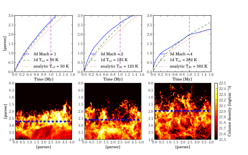
Figure 1: Top: Position (relative to the top of the box) of the mean ionization front as a function of time for the 3D turbulent simulations (respectively at Mach 1, 2, and 4 in solid-blue) of Tremblin et al. (2012) and the corresponding analytical solutions (red-dotted) and 1D simulations (green-dashed) in which the turbulence is taking into account by an effective temperature/sound speed. Bottom: snapshots of the column density of the 3D simulations at 1 Myr after the ionization is switched on at the top of the box. The blue-dashed lines show the mean position of the ionization front.

The expansion of 1D, spherical H ii regions in a homogeneous medium is a theoretical exercise whose first solution was proposed by Spitzer (1978) and Dyson & Williams (1980). Their solution can be written in terms of the initial Strömgren radius $r_{s}$:

$$r_{s} = (3S_{*}/4\pi n_{0}^{2}\alpha)^{1/3}$$ (1)

$$c_{II}t/r_{s} = 4/7\times((r/r_{s})^{7/4}-1)$$ (2)

$$P_{II} = n_{0}(r_{s}/r)^{3/2}k_{b}T_{II}$$ (3)

where $S_{*}$ is the production rate of ionizing photons, $n_{0}$ the gas density of the initial homogeneous medium, $\alpha$ the recombination rate, $c_{II}$ and $T_{II}$ the sound speed and temperature in the ionized gas. Although this solution is accurate at early times, it is obviously wrong for very long times since the radius of the ionized bubble would diverge to infinity. The radius cannot increase indefinitely because the expansion is driven by the ionized gas pressure that decreases like $r^{-3/2}$ (see Eq. 1) and the expansion will stop when this pressure reaches the pressure of the external medium (neglected in the solution given by Eq. 1). A simulation of this phenomenon can be found in Tremblin et al. (2011) (Fig. 1).

Recently, Raga et al. (2012) proposed a new 1D spherical analytical solution of the expansion of H ii regions that takes into account the post-shock material (and therefore the pressure of the external medium) in the equation of motion of the ionization front:

$$\frac{1}{c_{II}}\frac{dr}{dt}=\left(\frac{r_{s}}{r}\right)^{\beta}-\frac{c_{0}^{2}}{c_{II}^{2}}\left(\frac{r}{r_{s}}\right)^{\beta}$$ (4)

where $c_{0}$ is the sound speed in the initial medium, and $\beta$ is equal to 3/4 for a spherical geometry. Neglecting the last term in Eq. 4 gives back the equation derived by Spitzer (1978) and Dyson & Williams (1980), for which no equilibrium is possible. However, equating Eq. 4 to zero gives immediately an equilibrium radius $r_{eq}=r_{s}(c_{II}/c_{0})^{4/3}$ which corresponds to an ionization and hydrostatic equilibrium for which the pressure of the ionized gas $P_{II}$ is equal to the pressure of the surrounding medium $P_{0}$. Raga et al. (2012) compared this solution to 1D spherical simulations and they both agree relatively well especially at late times. However, in the simulation, the region overshoots the equilibrium radius before converging back to it. This effect is not present in the analytical solution and could be a consequence of the inertia of the shell that is neglected in the analytical derivation.

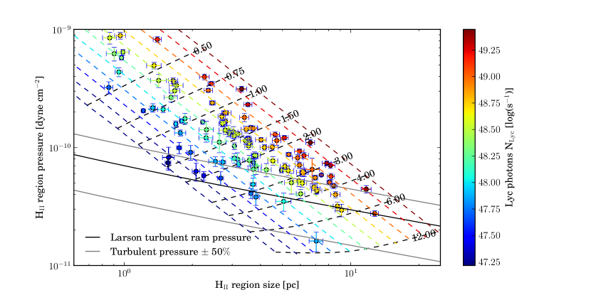
Figure 2: Pressure of the H ii regions of the HRDS survey as a function of radius. The black line is the turbulent ram pressure evaluated from Larson laws, at the scale of the radius of the region (Eq. 16). The grey lines show the limits at $\pm$ 50% of this relation. The dashed-colored lines are 1D simulations performed in a density and temperature profile based on Larson laws at different Lyc fluxes given by the colorbar. The dashed-black lines are isochrones (in Myr) built from these simulations, they are used to estimate the age of the H ii regions. To avoid a 3D plot, we assume an constant electron temperature of 8000 K for all the regions and simulations (only for this plot).

It has been thought for a long time that this equilibrium cannot be reached in large and diffuse H ii regions, because it would take much longer than the lifetime of the ionizing sources to reach it. However, although the thermal pressure of the initial medium cannot compensate the ionized gas pressure at early times, Tremblin et al. (2012) showed that the turbulent ram pressure can do the job. We recall this result in Fig. 1. The bottom panels show snapshots at 1 Myr of the column density of three different 3D simulations of the ionization of a turbulent medium respectively with an initial turbulence of Mach 1, 2, and 4. All the simulations were performed with HERACLES (Audit et al., 2011). The box is 4 pc³ at a resolution of 400³, the ionizing flux at the top of the box is plane-parallel $F_{*}$ = 10⁹ ph s^-1 cm^-1, the averaged density is $n_{0}$ = 500 cm^-3, and there is no gravity in these runs.

The turbulence investigated here is relatively moderate since one can expect a turbulence up to Mach 10 from the Larson’s law at this scale (see Larson, 1981). The blue-dashed line in Fig. 1 represents the mean position of the ionization front in the simulations and it does show that the ionization front is slowed down by the supersonic turbulence. In order to quantify this effect, we adapted Eq. 4 to a plane-parallel geometry ($\beta$ is equal to 1/4) and the equation still has an analytical solution:

$$r_{s} = F_{*}/n_{0}^{2}\alpha$$ (5)

$$c_{II}t/r_{s} = f(r/r_{s},c_{0}^{2}/c_{II}^{2})-f(1,c_{0}^{2}/c_{II}^{2})$$ (6)

$$f(x,a) = 4\tanh^{-1}(\sqrt{a}x^{1/4})/a^{5/2}-4x^{1/4}/a^{2}-4x^{3/4}/3a$$ (7)

To take into account the turbulence, we replaced the initial temperature $T_{0}$ in the sound speed $c_{0}$ by an effective turbulent temperature:

$$T_{eff}=\langle T_{0}+(\mu m_{H}/k_{b})\sigma_{0}^{2}/3\rangle_{\mathrm{box}}$$ (8)

where $\mu$ is the mean molecular weight, $T_{0}$ and $\sigma_{0}$ the temperature and velocity field of the simulation before the ionization starts, and the rms average is computed on the whole box. A discussion on the use of an effective turbulent temperature/sound speed can be found in Mac Low & Klessen (2004). Figure 1 shows the time evolution of the mean position of the ionization front in the 3D simulations, the position given by the analytical solution and the position of the front in 1D plane-parallel simulations with the effective turbulent temperature. The analytical solution and the 1D simulations capture quite well the slowing down of the ionization front caused by the turbulence at late times. At early times, the ionization front in the 3D simulations propagates faster with increasing turbulent levels. This is easy to understand: a larger turbulence results in denser structures and since the total amount of material is fixed in the box, this implies more low density parts. The average initial Strömgren radius computed on the varying density field in the 3D runs increases with the turbulent level because there are more and more low density parts for which the Strömgren radius will be large. In the analytical solutions and 1D simulations, the initial Strömgren radius is computed on the average density field, which is constant at n₀ = 500 cm^-3. Nevertheless, at later times, the initial conditions do not matter so much anymore, and the 3D simulations show a slowing down of the propagation of the ionization front as the analytical solutions and the 1D simulations.

A direct consequence of this analysis is that an H ii region will be able to expand in a turbulent medium while $P_{II}\geq P_{\mathrm{turb}}$ until the point where the two pressures equilibrates. It can be seen with the effective temperatures in Fig. 1 that the turbulent ram pressure can be easily one order of magnitude bigger than the thermal pressure. Therefore it is possible that some regions are in equilibrium with their turbulent environment before the ionizing stars explode.

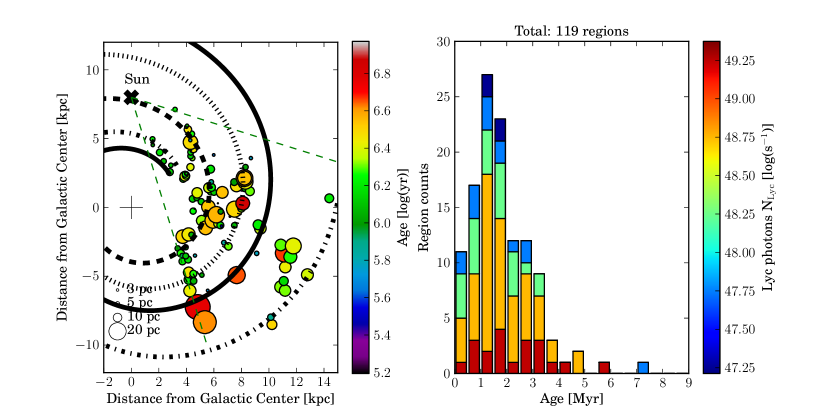
Figure 3: Left: Diameter, age, and position of the H ii regions of the HRDS survey in the Galaxy. The green dashed lines show the limit of the survey, the black thick curves are the position of the spiral arms of our Galaxy based on Russeil (2003). The ages are estimated using the grid of 1D simulations at a fixed density at 1pc (3400 cm^-3) for the initial profile. The galactic electron temperature gradient is taken into account using Eq. 12. Right: age distribution of our sample, the ionizing flux of the regions is indicated by the color scale.

3 HRDS survey and turbulent ram pressure from Larson’s laws

Using radio continuum surveys of H ii regions, it is possible to test that $P_{II}\geq P_{\mathrm{turb}}$ and to see if the equilibrium is reached for some regions. We used the H ii Region Discovery Survey (HRDS) made with the Green Bank Telescope at 9 GHz whose beam size is 82^′′ (see Anderson et al., 2011). The ionizing flux $S_{*}$ and the rms electron density $\langle n_{II}\rangle$ in a region can be computed by using the radio continuum integrated flux (see Martín-Hernández et al., 2005):

$$\langle n_{II}\rangle=\frac{4.092\times 10^{5}\mathrm{cm}^{-3}}{\sqrt{b(\nu,T_{e})}}\left(\frac{S_{\nu}}{\mathrm{Jy}}\right)^{0.5}\left(\frac{T_{e}}{10^{4}\mathrm{K}}\right)^{0.25}\left(\frac{D}{\mathrm{kpc}}\right)^{-0.5}\left(\frac{\theta_{D}}{{}^{\prime\prime}}\right)^{-1.5}$$ (9)

$$S_{*}=\frac{7.603\times 10^{46}\mathrm{s}^{-1}}{b(\nu,T_{e})}\left(\frac{S_{\nu}}{\mathrm{Jy}}\right)\left(\frac{T_{e}}{10^{4}\mathrm{K}}\right)^{-0.33}\left(\frac{D}{\mathrm{kpc}}\right)^{2}$$ (10)

$$b(\nu,T_{e})=1+0.3195\log\left(\frac{T_{e}}{10^{4}\mathrm{K}}\right)-0.2130\log\left(\frac{\nu}{\mathrm{GHz}}\right)$$ (11)

where $S_{\nu}$ is the radio continuum integrated flux at frequency $\nu$, $\theta_{D}$ is the angular diameter of the source, $D$ the distance from the Sun, and $T_{e}$ the electron temperature in the ionized plasma.

We deconvolved the beam size of the telescope (82$"$) from the full width at half maximum (FWHM) of the flux given in the HRDS survey. The HRDS survey provides a complexity flag that indicates whether the region has a peaked well-defined emission or a complex multi-component one. We exclude complex regions because the peak of the emission is not representative of the position of the ionizing sources, therefore the size of the region is likely to be wrong. These errors can be corrected with a careful look at the distribution of the radio emission (e.g. this is done for Rosette and RCW79 in Sect. 4, their emission has the shape of an annulus) but cannot be done automatically. This selection gives us a sample of 119 regions for which the ionizing flux and the rms electron density can be evaluated. Finally we converted the FWHM into the 1/e² width (FWHM$\times$1.7) to have the angular diameter of the region.

If not measured, $T_{e}$ can be inferred from the galacto-centric distance of the source $R_{\mathrm{gal}}$:

$$T_{e}=278\mathrm{K}\left(\frac{R_{\mathrm{gal}}}{\mathrm{kpc}}\right)+6080\mathrm{K}$$ (12)

This linear relation is an average value of the two samples studied in Balser et al. (2011) and the average value for the HRDS sample is 8000 K. The ionized gas pressure is then given by:

$$P_{II}=2\langle n_{II}\rangle k_{b}T_{e}$$ (13)

We estimated the turbulent ram pressure using Larson’s laws (see Larson, 1981). Of course the result will be scale-dependent, and one has to infer which scale is going to matter when trying to compute this ram pressure. In Sect. 2, we used the scale of the box to compute the effective sound speed. For the spherical H ii regions, we make the assumption that the radius of the region is the scale below which motions will act as an extra pressure against the expansion. Therefore taking the Larson relations:

$$\langle\sigma\rangle = 1.1\mathrm{km/s}\left(\frac{r}{\mathrm{pc}}\right)^{0.38}$$ (14)

$$\langle n\rangle = 3400\mathrm{cm}^{-3}\left(\frac{r}{\mathrm{pc}}\right)^{-1.1}$$ (15)

we evaluated the turbulent ram pressure at the scale of the radius of the region:

$$P_{\mathrm{turb}}\approx\langle\rho\rangle(c_{0}^{2}+\langle\sigma\rangle^{2}/3)$$ (16)

with $\langle\rho\rangle$ the rms density in g/cm³ and $c_{0}$ the sound speed (0.2 km/s). This relation is plotted in Fig. 2 with the ionized gas pressure $P_{II}$ of the regions in the HRDS survey evaluated from Eq. 13. There is of course a large scatter around the Larson’s relations and uncertainties concerning the right scale that should be used. Possible variations around this relations have been investigated in Lombardi et al. (2010) (see also Hennebelle & Falgarone, 2012). Therefore we also plot in Fig. 2 the ram pressure at $\pm$ 50%. Overall the pressure of the H ii regions is greater than the turbulent ram pressure of the surrounding medium, meaning that they are indeed able to expand in the turbulent medium. This is consistent with what we infer from the numerical simulations in Sect. 2. Furthermore, around 20% of our sample have pressures at $\pm$ 50 % of the turbulent ram pressure at the scale of their radius. This suggests that contrary to the usual picture, these regions may reach the limit of their expansion phase and may be in equilibrium with the surrounding turbulent medium.

4 Age estimation of the H ii regions

Based on the comparison in Sect. 2 between the 3D turbulent simulations and the 1D models with an effective turbulent temperature, we are confident in using 1D spherical simulations as a proxy to evaluate the age of the H ii regions. The coupled system of equation for 1D-spherical hydrodynamics coupled with ionization/recombination assuming the on-the-spot approximation is given by

$$\frac{\partial\rho}{\partial t} + \frac{1}{r^{2}}\frac{\partial}{\partial r}\left(r^{2}\rho u_{r}\right)=0\quad,$$ (17)

$$\frac{\partial n_{H}X}{\partial t} + \frac{1}{r^{2}}\frac{\partial}{\partial r}\left(r^{2}n_{H}Xu_{r}\right)=n_{H}(1-X)\sigma_{\gamma}F_{\gamma}-\alpha X^{2}n_{H}^{2}\quad,$$ (18)

$$\frac{\partial\rho u_{r}}{\partial t} + \frac{1}{r^{2}}\frac{\partial}{\partial r}\left(r^{2}\rho u_{r}^{2}\right)=-\frac{\partial p}{\partial r}\quad,$$ (19)

$$\frac{\partial E}{\partial t} + \frac{1}{r^{2}}\frac{\partial}{\partial r}\left(r^{2}(E+p)u_{r}\right)=n_{H}(1-X)\sigma_{\gamma}F_{\gamma}e_{\gamma}$$ (21)

$$\qquad\qquad\qquad\qquad-\alpha X^{2}n_{H}^{2}k_{b}T/(\gamma-1)\quad,$$

$$\frac{1}{r}\frac{\partial}{\partial r}\left(rF_{\gamma}\right) = n_{H}(1-X)\sigma_{\gamma}(-F_{\gamma}+F_{*}\delta_{0}(r-r_{*}))$$ (22)

where $\rho$, $u_{r}$, P, T, are the density, velocity, pressure, and temperature of the fluid, $E$ is the total energy given by $E=\rho u_{r}^{2}/2+e$, $X$ the ionization fraction given by $n_{H^{+}}/n_{H}$, $n_{H}$ the total hydrogen density $n_{H^{+}}+n_{H^{0}}$, $F_{\gamma}$ the ionizing flux, $\sigma_{\gamma}$ the ionization cross section, $e_{\gamma}$ the mean energy given by an ionizing photon to the gas, $\alpha$ the recombination rate, and $\gamma$ the adiabatic index. We assume an ideal gas to link the internal energy $e$ to the pressure: $p=e(\gamma-1)$. The system is splitted in a hydrodynamic step solved explicitly by a Godunov exact solver and an ionization/recombination step solved implicitly. We used a $\gamma$ of 1.001 so that the gas is locally isothermal in the absence of ionization/recombination processes.

We performed 1D spherical models in a medium with a density and pressure profile given by Eq. 14 and Eq. 16. When the ionized bubble expands in such a density/pressure profile, it will “feel” the turbulent ram pressure at a given radius acting against the expansion. A grid of models was computed with different fluxes (log₁₀(S_∗) between 47. and 51. in steps of 0.25), electronic temperature (T_e: 10⁴ K $\pm$ 50% in steps of 1000 K), and density at 1 pc ($n$(1pc): 3400 cm^-3 $\pm$ 50% in steps of 340 cm^-3). The simulation domain extends up to 25 parsec, we took a resolution of 2500 cells (uniformly spaced) and ran the simulations during 12 Myr. These models are plotted in Fig. 2 for a fixed electron temperature $T_{e}$ = 8000 K and a density at 1 pc of $n$(1pc) = 3400 cm^-3. In our final age estimation, we do take into account the electron temperature using Eq. 12, we used a fixed temperature in Fig. 2 to avoid a 3D plot for our grid of simulations, however we do take into account the electron temperature dependence for our final age estimation. The regions from the HRDS survey fall exactly on the simulated tracks at their ionizing fluxes. This is normal and a consequence of photon conservation that is assumed in Eq. 9 to evaluate $S_{*}$ from $\langle n_{II}\rangle$ and is also assumed in the simulations. It can be shown using photon conservation that $P_{II}\propto S_{*}^{0.5}r^{-1.5}$ (see Eq.1), which gives the linear tracks in log space for Fig. 9. The real contribution of the simulations are the isochrone curves built out of them (black-dashed lines). We can then estimate the dynamical age of the different regions.

Cloud ($D$)	Radius	$S_{\nu}(\nu)$	Phot. Age	Dyn. Age
[kpc]	[pc]	[Jy](GHz)	[Myr]	[Myr]
Rosette (1.6a)	18.7$\pm$1.2b	350(4.75)b	$\leq$ 5c	5.0$\pm$0.4
M16 (1.75d)	7.2$\pm$0.7e	117(5)e	2-3f	1.9$\pm$0.2
RCW79 (4.3g)	7.1$\pm$0.3h	19.5(0.84)h	2-2.5i	2.2$\pm$0.1
RCW36 (0.7j)	1.1$\pm$0.07e	30(5)e	1.1$\pm$0.6k	0.4$\pm$0.03

Table 1: H ii regions used for comparison between photometric and dynamical age. The fluxes are integrated radio continuum fluxes at the frequency indicated in parenthesis. The electron Temperature $T_{e}$ is determined from Eq. 12. ^a(Román-Zúñiga & Lada, 2008) ^b(Celnik, 1985) ^c(Martins et al., 2012) ^d(Guarcello et al., 2007) ^e (Condon et al., 1993) ^f(Hillenbrand et al., 1993) ^g(Russeil, 2003) ^h (Mauch et al., 2003) ⁱ(Martins et al., 2010) ^j(Yamaguchi et al., 1999) ^k(Ellerbroek et al., 2013)

We tested this method on well-known regions for which an independent age of the central massive OB stars is available from photometry and evolutionary tracks in the HR diagram. We took four regions: Rosette, M16, RCW79, and RCW36, their parameters and the corresponding references are given in Tab. 1. For all the regions, we used Eq. 12 to estimate the electron temperature. Our age estimations are in good agreement with the ages derived from photometry, however some questions can be raised:

• In the case of the Rosette Nebula, Martins et al. (2012) concluded that the age of the two most massive O stars in NGC2244 is less than 2 Myr, however they suggest that either there is a bias in their effective temperature, or they were the last to form. For the second possibility, the H ii region would be powered first by the lower-mass O stars, and then by the two most massive ones that dominate the total ionizing flux. The ionizing flux is thus a function of time in that case, and could change the dynamical age. The same may also happen for the future development of RCW79 with the appearance of a compact and younger H ii region at the southeast of the region.

• The dynamical age of RCW36 is at the lower end of the photometric range. This could mean that the ionizing O star is also the last to form. However contrary to the Rosette Nebula, we do not expect a two-stage expansion in this case because there is only one dominant ionizing source. Other physical phenomena at the early stages of the expansion could also delay the expansion by 0.1-0.2 Myr. (see Sect. 5.1).

In Sect. 5.2, we will discuss in further detail the possible biases of our approach. However, considering the uncertainties and the error bars of the age derived from evolutionary stages, the dynamical age agrees well. Besides, it has the advantage of being much simpler to compute and can be applied to a large sample of OB associations. We apply the method on the HRDS sample and give the age distribution in the right panel of Fig. 3. The average age of the 119 regions is 1.9 Myr $\pm$ 0.7 Myr. The distribution is plotted as a stacked histogram indicating the ionizing flux of the sources and we do not see any trend as a function of flux. There is a tail with older regions that is not very well sampled, probably because there are not many big and bright sources such as the Rosette Nebula in the survey. The average age of the sample is relatively small compared to the typical lifetime of a massive star (30 Myr for a typical B-type star of 10 M_⊙). The left panel of Fig. 3 shows the size, age and position of the regions in the Galaxy. The Scutum-Crux arm (dash-dotted spiral) has been extended beyond the distance constrained in Russeil (2003), this is probably why the most distant regions do not lie very well on the arm. At first sight, the regions in the Sagittarius-Carina arm (dashed spiral) seem younger than the regions in the other arms, however most of these regions are also the closest to the Sun so the completeness and sensitivity limits of the survey have to be carefully studied before making any firm conclusion.

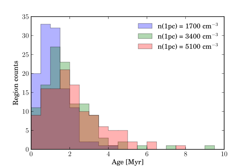
Figure 4: Effect of changing by $\pm$ 50% the density at 1 pc of the initial density profile on the total age distribution. Note that this effect is applied to all the regions, in reality it should not be such a systematic positive or negative bias.

5 Discussion

5.1 What about gravity and magnetic fields ?

Other physical phenomena could also affect the expansion of the ionization front and balance the ionized gas pressure. Their associated pressure should be compared to the turbulent pressure given by Eq. 16 and with the ionized-gas pressure in Eq. 1. The effect of self gravity is negligible on the expansion because of Gauss’s law for gravity. Only the mass of the ionized gas will act at the ionization front (however the gas self gravity is an important effect to consider when studying the compression in the shell). The gravity of the central cluster could play a role. If we assume that an hydrostatic equilibrium is possible, we have the relation:

$$P_{II}-P_{0} = \int^{\infty}_{r}\frac{GM\rho(r^{\prime})}{r^{\prime 2}}dr^{\prime}\quad\mathrm{with}\quad\rho(r^{\prime})=\rho(1\mathrm{pc})\left(\frac{r^{\prime}}{\mathrm{pc}}\right)^{-1.1}$$ (23)

$$P_{II} \approx P_{G}\approx\frac{GM\rho(1\mathrm{pc})}{2.1\times(1\mathrm{pc})}\left(\frac{r}{\mathrm{pc}}\right)^{-2.1}$$ (24)

where $M$ is the mass of the central cluster. Assuming a cluster mass of 500 M_⊙ gives a gravitational pressure on the order of 1.62$\times$10^-10 dyne cm^-2 at one parsec, which is comparable to the turbulent pressure at that scale (see Fig. 2). Nevertheless, this pressure is dropping much faster than the turbulent pressure ($\approx$ r^-2), therefore if expansion has happened at some point with $P_{II}$ $\geq$ $P_{G}$, the gravity of the central cluster will never be able to stop the large-scale expansion in the future. However, gravitational effects can be important at small scales for compact and ultra-compact H ii regions (see Keto, 2007; Peters et al., 2010), therefore we do not expect our model to apply for spatial scale smaller than $\approx$ 0.1 pc (and age smaller than 0.1-0.2 Myr).

The magnetic pressure could also play a role. Assuming a constant mass to flux ratio in molecular clouds and a typical magnetic field of 20 $\mu G$ at one parsec (see Troland & Crutcher, 2008; Lazarian et al., 2012), we can derive the scaling relation (for larger scales):

$$\frac{\langle\phi\rangle}{\phi(1\mathrm{pc})} = \frac{\langle M\rangle}{M(1\mathrm{pc})}\rightarrow\frac{\langle B\rangle}{B(1\mathrm{pc})}\times\left(\frac{r}{\mathrm{pc}}\right)^{2}=\frac{\langle\rho\rangle}{\rho(1\mathrm{pc})}\times\left(\frac{r}{\mathrm{pc}}\right)^{3}$$ (25)

$$\langle B\rangle = 20\mu G\left(\frac{r}{\mathrm{pc}}\right)^{-0.1}\quad\mathrm{and}\quad P_{B}=\frac{\langle B\rangle^{2}}{8\pi}$$ (26)

At one parsec, this magnetic field leads to a magnetic pressure on the order of 1.5$\times$10^-11 dyne cm ^-2, much smaller than the turbulent pressure. Even if the magnetic pressure inside the H ii region acts as a support, its strength is small compared to the ionized-gas pressure. Therefore the magnetic field pressure does not have an important effect for the large scale evolution of H ii regions. However, Crutcher (2012) showed that the magnetic field can be on the order of 100-1000 $\mu G$ for dense gas at small scales, consequently the small-scale evolution of H ii regions could depend on the magnetic field.

Both gravity and magnetic fields should be considered for the evolution of compact and ultra-compact H ii regions but should not affect the large-scale evolution of diffuse nebulae. The presence of dust can also have an important effect for small regions (see Inoue, 2002; Arthur et al., 2004). As a consequence, we do not expect our models to be able to predict the ages for small regions at a scale of 0.1 pc and the error bars for regions around 1 pc are possibly larger because of the uncertainties in the small scale evolution.

5.2 The effect of initial conditions

Environmental variations in the surrounding density can also be an issue. We managed to correct for the electron temperature but we did not take into account possible variations of the density profile around the one given by Eq. 14. Our grid of simulations can take into account such variations (up to $\pm$ 50% around $n$(1pc) = 3400 cm^-3) but we do not have observational constraints for the local density around the regions of the HRDS survey. To illustrate the effect of the density variations, we recomputed the age distribution of Fig. 3 for $n$(1pc) = 1700 cm^-3 and 5100 cm^-3. The corresponding distributions are given in Fig. 4. For $n$(1pc) = 1700 cm^-3, the distribution is shifted at 1.4 Myr $\pm$ 0.8 Myr, and for $n$(1pc) = 5100 cm^-3 at 2.3 Myr $\pm$ 0.8 Myr. The changes are significant, but we do not expect the local variation in the density at one parsec to be systematically positive or negative for all regions so that we would have to shift the global Larson’s law accordingly. Therefore the average age of the distribution should remain relatively constant and the variations around the density at one parsec may only increase the standard deviation. Furthermore, we do not expect the bias caused by the density variations to be important for the large regions. Indeed, large regions have a surrounding area big enough to recover an average density that should be relatively close to what can be inferred from Larson’s relation. For smaller regions ($\approx$ 1 pc), the local density variations can be important and lead to different ages. However, if enough regions are included in the statistics, the age distribution should be fairly good although the age estimation of a small particular region might be wrong.

5.3 Advantages of dynamical age determinations and perspectives

The dynamical evolution inferred from our grid of models is a good way to get an estimation of the age of the OB associations, especially when we consider how difficult and uncertain it is to get it from photometry and evolutionary tracks. In principle 3D simulations would be required to study the evolution in a turbulent medium but, they are currently too time-consuming to allow the computation of a full grid of models as a function of flux, temperature and density. Thanks to the equivalent grid of 1D simulations, the method is relatively cheap and we can take into account the environmental dependences.

Although this method cannot be used for small regions for which magnetic fields and gravity have to be considered, we can easily date a large sample of diffuse H ii regions when they can be resolved and their Lyc flux estimated in observations. This method could also be applied to nearby extra-galactic H ii regions, thus allowing us to get age distributions of massive-star forming regions in other galaxies. These distributions could then be used to constrain galaxy-scale simulations of star formation.