Toward optimal cluster power spectrum analysis

Abstract

The power spectrum of galaxy clusters is an important probe of the cosmological model. In this paper we develop a formalism to compute the optimal weights for the estimation of the matter power spectrum from cluster power spectrum measurements. We find a closed-form analytic expression for the optimal weights, which takes into account: the cluster mass, finite survey volume effects, survey masking, and a flux limit. The optimal weights are: $w(M,\chi)\propto b(M,\chi)/[1+\bar{n}_{\rm h}(\chi)\overline{b^{2}}(\chi)\overline{P}(k)]$, where $b(M,\chi)$ is the bias of clusters of mass $M$ at radial position $\chi(z)$, $\bar{n}_{\rm h}(\chi)$ and $\overline{b^{2}}(\chi)$ are the expected space density and bias squared of all clusters, and $\overline{P}(k)$ is the matter power spectrum at wavenumber $k$. This result is analogous to that of Percival et al. (2004). We compare our optimal weighting scheme with mass weighting and also with the original power spectrum scheme of Feldman et al. (1994). We show that our optimal weighting scheme outperforms these approaches for both volume- and flux-limited cluster surveys. Finally, we present a new expression for the Fisher information matrix for cluster power spectrum analysis. Our expression shows that for an optimally weighted cluster survey the cosmological information content is boosted, relative to the standard approach of Tegmark (1997).

1 Introduction

The number counts of massive galaxy clusters has long been known to provide strong constraints on the cosmological model, provided one understands how to map from observed mass proxies to a theoretical halo mass (for a recent review see Allen et al., 2011). Since the first measurements of the clustering of Abell clusters was performed in the 70’s and early 80’s, it has been understood that the clustering of clusters contains additional vital information about the cosmological model (Hauser & Peebles, 1973; Bahcall & Soneira, 1983). In particular, these studies were able to show that the clustering of clusters was stronger than that of the galaxies. This quickly lead to the realization that galaxies and clusters could not both be unbiased tracers of the mass distribution (Kaiser, 1984). One of the major attractions of the cold dark matter (hereafter, CDM) framework, is that ‘biased’ clustering naturally emerges within it. In Kaiser’s seminal work, he showed that the peaks and troughs of a Gaussian random field were correlated more strongly than the correlation function of the unconstrained field. Under the assumption that the Abell clusters formed out of the high peaks of a Gaussian Random Field one would then expect the Abell clusters to be more strongly correlated than galaxies. Further theoretical support comes from the excursion set formalism, which showed that initially overdense patches of a CDM universe would collapse to form dark matter haloes, and that these would, in general, be positively biased with respect to the underlying matter (Cole & Kaiser, 1989; Mo & White, 1996; Sheth & Tormen, 1999). One important consequence of these developments was that in the mid 90s, it was also realized that, if one combined measurements of the clustering of clusters with measurements of their abundances, one could break the degeneracies in cosmological parameters that were inherent in one single method (Mo et al., 1996; Majumdar & Mohr, 2004; Lima & Hu, 2004, 2005; Oguri, 2009; Cunha et al., 2010; Smith & Marian, 2011; Oguri & Takada, 2011).

Some notable measurements of the clustering of clusters are: in the X-rays, initial measurements of the cluster correlation function for ROSAT data were performed by Romer et al. (1994), and were later improved upon by Collins et al. (2000) using the 344 clusters in the REFLEX survey (see also Abadi et al., 1998, for results from the XBACS survey). In the optical, cluster samples tend to be orders of magnitude larger (for a review of early results see Bahcall, 1988). The APM galaxy survey was able to identify several hundred clusters for which clustering was computed (Dalton et al., 1992; Miller et al., 2001; Miller & Batuski, 2001). In the past decade, the Sloan Digital Sky Survey (SDSS) has produced, by far, the largest homogeneous sample of optical clusters: the MaxBCG sample whose clusters are detected via the ‘red sequence’ cluster detection method in multi-band imaging data (Koester et al., 2007). This sample contains 13,823 clusters with velocity dispersions $\gtrsim$400 ${\rm km\,s}^{-1}$ and covers an area of $\gtrsim 7000$ square degrees. The cluster correlation functions were explored by Bahcall et al. (2003) and Estrada et al. (2009), and the power spectrum analysis was performed by Hütsi (2010).

In the future, X-ray cluster surveys, such as eROSITA, should produce homogeneous cluster samples with numbers of clusters on the order of $\sim$100,000 (Pillepich et al., 2012). Deep multi-band optical surveys such as the Dark Energy Survey should also produce tens of thousands of high signal-to-noise ratio (hereafter, ${\mathcal{S}}/{\mathcal{N}}$) clusters. The question then arises: how should one perform an optimal measurement of the clustering of galaxy clusters? In a series of recent theoretical studies (Seljak et al., 2009; Hamaus et al., 2010), it was claimed that if galaxy clusters were weighted by a function with a linear dependence on mass, then the shot-noise on cluster power spectra measurements would be significantly reduced, hence yielding improved cosmological information. A complex study by Cai et al. (2011), proposed that the optimal way to reconstruct the mass distribution from a set of clusters was to weight the galaxy clusters by some combination of their mass and bias. In the limit of a low mass detection threshold for the clusters, these works lead to the conclusion that weighting by mass results in a maximal ${\mathcal{S}}/{\mathcal{N}}$ measurement of the matter density fluctuations. However, the caveat to the above analysis was that neither work directly demonstrated that the ${\mathcal{S}}/{\mathcal{N}}$ for cluster power spectra would be maximized. In this paper we shall directly perform this task. As we shall show, our analysis generalizes the galaxy power spectrum methods developed by Feldman et al. (1994, hereafter FKP) and Percival et al. (2004, hereafter PVP).

This paper is broken down as follows: In §2 we overview the specifications of a cluster survey, the construction of the density field of clusters, and its basic statistical properties. In §3 we detail the estimators of the two-point correlation function and the power spectrum. In §4 we write down the covariance matrix of the power spectrum estimator in the most general form and the Gaussian limit. In §5 we provide details of the derivation of the optimal weighting scheme. In §6 we compare various weighting schemes with our optimal weights for the cases of volume limited and flux-limited cluster surveys. We also present a new expression for the Fisher information matrix, which may be used for predicting the cosmological information content of optimally weighted measurements of the cluster power spectrum. Finally, in §7 we summarize our findings and conclude.

2 Survey specifications and the ${\mathcal{F}}_{\rm c}$–field

2.1 A generic cluster survey

Let us begin by defining our fiducial cluster survey: suppose that we have observed $N$ clusters and to the $i$th cluster we assign a mass $M_{i}$, redshift $z_{i}$ and angular position on the sky $\bm{\Omega}_{i}=\bm{\Omega}(\theta_{i},\phi_{i})$. The cluster selection function depends on both position and cluster mass and in general, is a complex function of the survey flux limit, and the cluster detection procedure (for an example of the complexities involved in computing this for the eROSITA mission see Pillepich et al., 2012). However, it may be simplified in the following ways. Firstly, provided the flux-limit is homogeneous across the survey area, the angular and radial parts of the selection function are separable:

$$\Theta({\bf x}|M)=\Theta(\bm{\Omega})\Theta(\chi|M),$$ (1)

where $\chi=\chi(z)$ is the radial comoving geodesic distance to redshift $z$. The angular selection function may be written:

$$\Theta(\bm{\Omega})=\left\{\begin{array}[]{cc}1\ ;&[{\bm{\Omega}}\in{\bm{\Omega}}_{\mu}]\\ 0\ ;&[\rm otherwise]\end{array}\ ,\right.$$ (2)

where $\bm{\Omega}_{\mu}$ defines the survey mask. The radial selection function may be written:

$$\Theta(\chi|M)=\left\{\begin{array}[]{cc}1\ ;&[{\chi}\in\chi_{\rm max}(M)]\\ 0\ ;&[\rm otherwise]\end{array}\ ,\right.$$ (3)

where $\chi_{\rm max}(M)$ is the maximum comoving geodesic distance out to which a cluster of mass $M$ could have been detected. This last relation may be inverted to obtain a very useful relation, which is the minimum detectable cluster mass at radial position $\chi(z)$ in the survey. We shall denote this quantity as $M_{\rm Lim}(\chi)$.

Secondly, if the survey is volume limited, the minimum detectable mass is independent of position and we may write:

$$\Theta^{\rm VL}(\chi|M)=\Theta^{\rm VL}(\chi)\Theta^{\rm VL}(M)\ ,$$ (4)

where

$$\Theta^{\rm VL}(\chi|M)=\left\{\begin{array}[]{cc}1\ ;&[{\chi}\leq\chi_{\rm max}]\\ 0\ ;&[\rm otherwise]\end{array}\ \right.\hskip 28.45274pt\ ;\hskip 28.45274pt\Theta^{\rm VL}(M)=\left\{\begin{array}[]{cc}1\ ;&[M\geq M_{\rm Lim}]\\ 0\ ;&[\rm otherwise]\end{array}\ .\right.$$ (5)

The survey volume may now be defined as the integral of the selection function over all space:

$${V_{\mu}}(M)=\int^{\chi_{\rm max}(M)}_{0}\Theta({\bf x}|M)dV(\chi,\bm{\theta})=\Omega_{\mu}\int_{0}^{\chi_{\rm max}(M)}d\chi D^{2}_{A}(\chi),$$ (6)

where $dV(\chi,\bm{\theta})$ is the comoving volume element at position vector ${\bf x}(\chi(z),\bm{\theta})$, $D_{A}(\chi)$ is the comoving angular diameter distance. For a flat space-time geometry the survey volume simplifies to,

$${V_{\mu}}(M)=\frac{\Omega_{\mu}}{3}\chi_{\rm max}^{3}(M)\ .$$ (7)

2.2 The cluster delta expansion

In general the spatial density distribution of clusters, per unit mass, at position ${\bf x}(\chi,\bm{\Omega})$ may be written as a sum over Dirac delta functions:

$$n_{{\rm c}}(M,{\bf x})=\sum_{i=1}^{N}\delta^{\rm D}(M-M_{i})\delta^{\rm D}({\bf x}-{\bf x}_{i})\ .$$ (8)

If the selection function is inhomogeneous, then the mean density of clusters varies spatially over the survey. Next, in analogy with PVP, we define a field ${\mathcal{F}}_{\rm c}$, which is related to the over-density of clusters. This can be written:

$${\mathcal{F}}_{\rm c}({\bf x})=\int dM\frac{w({\bf x},M)}{\sqrt{A}}\Theta({\bf x}|M)\left[n_{{\rm c}}({\bf x},M)-\alpha n_{s}({\bf x},M)\right]\ ,$$ (9)

where $n_{s}({\bf x},M)$ represents the number density of clusters in a mock sample that has no intrinsic spatial correlations, and whose density is $1/\alpha$ times that of the true cluster field at that mass. Note that whilst the field $n_{s}({\bf x},M)$ has no intrinsic spatial correlations it does possess a spectrum of masses, which is closely related to the mass spectrum of the field $\left<n_{{\rm c}}({\bf x},M)\right>$. The choice for the normalization parameter $A$ will be given later. The quantity $w({\bf x},M)$ denotes a weight function that, in general, may depend on both the spatial position and mass of the cluster. It is this quantity that we shall aim to determine in an optimal way.

2.3 Statistical properties of the cluster density field

Determination of the optimal weight function will require statistical analysis on the field ${\mathcal{F}}_{\rm c}$, therefore we will now introduce the necessary tools. As a simple example let us compute the ensemble average value of the field ${\mathcal{F}}_{\rm c}$, which can be written,

$$\left<{\mathcal{F}}_{\rm c}({\bf x})\right>=\int dM\frac{w({\bf x},M)}{\sqrt{A}}\Theta({\bf x}|M)\left[\left<n_{{\rm c}}({\bf x},M)\right>-\alpha\left<n_{s}({\bf x},M)\right>\right]\ ,$$ (10)

where the angled brackets denote an ensemble average in the following sense:

$$\left<B(\left\{{\bf x}_{i},M_{i}\right\})\right>\equiv\int{\rm d}{\bf x}_{1}\dots\rm d{\bf x}_{N}{\rm d}M_{1}\dots\rm dM_{N}p({\bf x}_{1},\dots,{\bf x}_{N},M_{1},\dots,M_{N})B(\left\{{\bf x}_{i},M_{i}\right\})\ .$$ (11)

in the above $p({\bf x}_{1},\dots,{\bf x}_{N},M_{1},\dots,M_{N})$ is the $N$-point joint probability distribution for the $N$ clusters being located at the set of spatial positions $\{{\bf x}_{i}\}$ and having the set of masses $\{M_{i}\}$. Thus, the first expectation on the right-hand side of Eq. (10) can be written as:

$$\left<n_{{\rm c}}({\bf x},M)\right>=\int\prod_{l=1}^{N}\left\{{\rm d}{\bf x}_{l}{\rm d}M_{l}\right\}p({\bf x}_{1},\dots,{\bf x}_{N},M_{1},\dots,M_{N})\sum_{i=1}^{N}\delta^{\rm D}({\bf x}-{\bf x}_{i})\delta^{\rm D}(M-M_{i})=\sum_{i=1}^{N}p({\bf x},M)=Np({\bf x},M)\ .$$ (12)

On the first line we inserted the expansion of the cluster density field from Eq. (8) and to obtain the second we integrated over the sum of Dirac delta functions. The quantity $p({\bf x},M)$ can be written in a more transparent way:

$$p({\bf x},M)\equiv p({\bf x})p(M)=\frac{1}{V}\frac{\bar{n}(M)}{N/V}=\frac{\bar{n}(M)}{N}\ ,$$ (13)

where $\bar{n}(M)$ is the intrinsic number density of clusters per unit mass – i.e. the dark matter halo mass function.

Turning to the second expectation value, we note that the only difference between $\left<n_{{\rm c}}({\bf x},M)\right>$ and $\left<n_{s}({\bf x},M)\right>$ is the artificially increased space density of clusters and the absence of any intrinsic clustering. Hence, we also have,

$$\alpha\left<n_{s}({\bf x},M)\right>=\bar{n}(M)\ .$$ (14)

Putting this all together, we arrive at the result:

$$\left<{\mathcal{F}}_{\rm c}({\bf x})\right>=0\ .$$ (15)

Hence the ${\mathcal{F}}_{\rm c}$–field, like the over-density field of matter, is a mean-zero field.

Note that we have neglected to take into account the statistical properties of obtaining the $N$ clusters in the survey volume. In what follows we shall assume that the survey volumes are sufficiently large that this may be essentially treated as a deterministic quantity. However, it can be taken into account (e.g. see Sheth & Lemson, 1999; Smith & Watts, 2005; Smith, 2009).

3 Clustering Estimators

3.1 An estimator for the two-point correlation function

The two-point correlation function of the field ${\mathcal{F}}_{\rm c}$ can be computed directly as:

$$\left<{\mathcal{F}}_{\rm c}({\bf x}_{1}){\mathcal{F}}_{\rm c}({\bf x}_{2})\right> = \frac{1}{A}\int dM_{1}dM_{2}w({\bf x}_{1},M_{1})w({\bf x}_{2},M_{2})\Theta({\bf x}_{1}|M_{1})\Theta({\bf x}_{2}|M_{2})\left[\frac{}{}\left<n_{\rm c}({\bf x}_{1},M_{1})n_{\rm c}({\bf x}_{2},M_{2})\right>\right.$$ (16)

$$\left.\frac{}{}-\alpha\left<n_{\rm c}({\bf x}_{1},M_{1})n_{s}({\bf x}_{2},M_{2})\right>-\alpha\left<n_{\rm c}({\bf x}_{2},M_{2})n_{s}({\bf x}_{1},M_{1})\right>+\alpha^{2}\left<n_{s}({\bf x}_{1},M_{1})n_{s}({\bf x}_{2},M_{2})\right>\right]\ .$$

The calculation of the above terms is detailed in the appendix A. On substituting the results of Eqs (71) and (72), we write

$$\xi_{{\mathcal{F}}_{\rm c}}({\bf x}_{1},{\bf x}_{2}) = \frac{1}{A}\int dM_{1}dM_{2}w({\bf x}_{1},M_{1})w({\bf x}_{2},M_{2})\bar{n}(M_{1})\bar{n}(M_{2})\Theta({\bf x}_{1}|M_{1})\Theta({\bf x}_{2}|M_{2})\xi^{\rm c}({\bf x}_{1},{\bf x}_{2},M_{1},M_{2})$$ (17)

$$+\;\;\frac{(1+\alpha)}{A}\int dMw^{2}({\bf x}_{1},M)\bar{n}(M)\Theta({\bf x}_{1}|M)\delta^{\rm D}({\bf x}_{1}-{\bf x}_{2})\ ,$$

where we defined $\xi_{{\mathcal{F}}_{\rm c}}({\bf x}_{1},{\bf x}_{2})\equiv\left<{\mathcal{F}}_{\rm c}({\bf r}_{1}){\mathcal{F}}_{\rm c}({\bf r}_{2})\right>$. Note that in the second line of the above equation we have benefited from the identity: $\Theta^{2}({\bf x}|M)=\Theta({\bf x}|M)$. If we assume that the cluster density field is some local function of the underlying dark matter density (Fry & Gaztanaga, 1993; Mo & White, 1996; Mo et al., 1997; Smith et al., 2007), the cross-correlation function of clusters of masses $M_{1}$ and $M_{2}$, at leading order, can be written:

$$\xi^{\rm c}(|{\bf x}_{1}-{\bf x}_{2}|,M_{1},M_{2})=b(M_{1})b(M_{2})\xi(|{\bf x}_{1}-{\bf x}_{2}|)\ ,$$ (18)

where $\xi(r)$ is the correlation of the underlying matter fluctuations. On inserting this relation into Eq. (17) we find:

$$\xi_{{\mathcal{F}}_{\rm c}}({\bf x}_{1},{\bf x}_{2})={\mathcal{G}}_{(1,1)}({\bf x}_{1}){\mathcal{G}}_{(1,1)}({\bf x}_{2})\xi(|{\bf x}_{1}-{\bf x}_{2}|)+(1+\alpha){\mathcal{G}}_{(2,0)}({\bf x}_{1})\delta^{D}({\bf x}_{1}-{\bf x}_{2})\ ,$$ (19)

where we have defined the weighted selection function

$${\mathcal{G}}_{(l,m)}({\bf x})\equiv\frac{1}{A^{l/2}}\int dM\bar{n}(M)b^{m}(M)w^{l}({\bf x},M)\Theta({\bf x}|M)\ .$$ (20)

One possible estimator for the matter correlation function from the ${\mathcal{F}}_{\rm c}$ field is therefore:

$$\hat{\xi}_{{\mathcal{F}}_{\rm c}}({\bf x})\equiv\int{\rm d}{\bf x}^{\prime}{\mathcal{F}}_{\rm c}({\bf x}){\mathcal{F}}_{\rm c}({\bf x}+{\bf x}^{\prime})\ \ \ ;\ \ \ ({\bf x}\neq{\bf 0})\ .$$ (21)

If we now compute the expectation of this estimator we find:

$$\left<\hat{\xi}_{{\mathcal{F}}_{\rm c}}({\bf x})\right>=\xi({\bf x})\int{\rm d}{\bf x}^{\prime}\,{\mathcal{G}}_{(1,1)}({\bf x}){\mathcal{G}}_{(1,1)}({\bf x}+{\bf x}^{\prime})\ \ \ ;\ \ \ ({\bf x}\neq{\bf 0})\ .$$ (22)

Although $\hat{\xi}_{{\mathcal{F}}_{\rm c}}({\bf x})$ is not an unbiased estimator of the matter correlation function, we may construct one that is:

$$\hat{\xi}_{0}({\bf x})\equiv\hat{\xi}_{{\mathcal{F}}_{\rm c}}({\bf x})/\Xi_{0}({\bf x})\hskip 8.5359pt;\hskip 8.5359pt\Xi_{0}({\bf x})\equiv\int{\rm d}{\bf x}^{\prime}\,{\mathcal{G}}_{(1,1)}({\bf x}){\mathcal{G}}_{(1,1)}({\bf x}+{\bf x}^{\prime})\ .$$ (23)

3.2 An estimator for the cluster power spectrum

We may now compute the Fourier space equivalent of the two-point correlation function, the power spectrum. In what follows we shall adopt the following Fourier transform conventions:

$$\tilde{B}({\bf k})=\int{\rm d}{\bf x}B({\bf x}){\rm e}^{i{\bf k}\cdot{\bf x}}\hskip 14.22636pt\Leftrightarrow\hskip 14.22636ptB({\bf x})=\int\frac{{\rm d}{\bf k}}{(2\pi)^{3}}{\tilde{B}}({\bf k}){\rm e}^{-i{\bf k}\cdot{\bf x}}\ .$$

We also define the power spectrum, $P_{B}(k)$, of any infinite statistically homogeneous random field $\tilde{B}({\bf k})$ to be:

$$\left<{\tilde{B}}({\bf k}){\tilde{B}}({\bf k}^{\prime})\right>\equiv(2\pi)^{3}\delta^{\rm D}({\bf k}+{\bf k}^{\prime})P_{B}({\bf k})\ .$$

Note that if the field $B$ were statistically isotropic, the power spectrum would simply be a function of the scalar $k$. With the above definitions in hand, the covariance of the Fourier modes of the cluster field ${\mathcal{F}}_{\rm c}$ can be written:

$$\left<\widetilde{\mathcal{F}}_{\rm c}({\bf k}_{1})\widetilde{\mathcal{F}}_{\rm c}({\bf k}_{2})\right> = \frac{1}{A}\int\prod_{i=1}^{2}\left\{{\rm d}{\bf x}_{i}dM_{i}w({\bf x}_{i},M_{i})\bar{n}(M_{i})\Theta({\bf x}_{i}|M_{i}){\rm e}^{{\bf k}_{i}\cdot{\bf x}_{i}}\right\}\xi^{\rm c}({\bf x}_{1},{\bf x}_{2},M_{1},M_{2})$$ (24)

$$+(1+\alpha)\int{\rm d}{\bf x}\,dM\bar{n}(M)\Theta({\bf x}|M)w^{2}({\bf x},M){\rm e}^{i({\bf k}_{1}+{\bf k}_{2})\cdot{\bf x}}\ .$$

For any infinite homogeneous random field, the two-point correlation function and the power spectrum form a Fourier pair, hence we may write:

$$\xi^{\rm c}({\bf x}_{1},{\bf x}_{2},M_{1},M_{2})=\int\frac{{\rm d}{\bf k}}{(2\pi)^{3}}P_{c}({\bf k},M_{1},M_{2}){\rm e}^{-i{\bf k}\cdot({\bf x}_{1}-{\bf x}_{2})}\ .$$

If we assume the linear biasing relation of Eq. (18), then the cross-power spectrum of clusters of different masses $M_{1}$ and $M_{2}$, at leading order, can be written

$$P_{c}({\bf k},M_{1},M_{2})=b(M_{1})b(M_{2})P({\bf k})\ ,$$ (25)

where $P({\bf k})$ is the matter power spectrum. On using these expressions in Eq. (24), and considering the case ${\bf k}_{1}=-{\bf k}_{2}$ we find:

$$\left<|\widetilde{\mathcal{F}}_{\rm c}({\bf k})|^{2}\right>=\int\frac{{\rm d}{\bf q}}{(2\pi)^{3}}P({\bf q})\left|\widetilde{\mathcal{G}}_{(1,1)}({\bf k}-{\bf q})\right|^{2}+P_{\rm shot}\ ,$$ (26)

where in the above expression $\widetilde{\mathcal{G}}_{(l,m)}({\bf k})$ is the Fourier transform of the weighted survey selection function from Eq. (20) and we have defined the shot-noise term as:

$$P_{\rm shot}\equiv(1+\alpha)\widetilde{\mathcal{G}}_{(2,0)}({\bf 0})\ .$$ (27)

Just as in the case of galaxies (Feldman et al., 1994), the expectation of the square amplitude of the Fourier modes of ${\mathcal{F}}_{\rm c}$ is given by the convolution of the matter power spectrum with the modulus square of the Fourier modes of the survey window function, plus a constant shot noise.

In the limit that the survey volume is large, the functions $\widetilde{\mathcal{G}}_{(l,m)}({\bf k})$ will be very narrowly peaked around ${\bf k}=0$. Provided the matter power spectrum is a smoothly varying function of scale, the window functions $\widetilde{\mathcal{G}}_{(l,m)}({\bf k})$ take on Dirac delta-function-like behaviour. Thus, in the large-survey volume limit, the first term on the right-hand side of Eq. (26) becomes:

$$\int\frac{{\rm d}{\bf q}}{(2\pi)^{3}}P({\bf q})\left|\widetilde{\mathcal{G}}_{(1,1)}({\bf k}-{\bf q})\right|^{2}\approx P({\bf k})\int\frac{{\rm d}{\bf q}}{(2\pi)^{3}}\left|\widetilde{\mathcal{G}}_{(1,1)}({\bf k}-{\bf q})\right|^{2}\ .$$ (28)

Let us focus on the integral factor on the right-hand-side of the above expression. Transforming the variable ${\bf k}-{\bf q}\rightarrow{\bf q}^{\prime}$ and using Parseval’s theorem, as well as Eq. (20), we find:

$$\int\frac{{\rm d}{\bf q}}{(2\pi)^{3}}\left|\widetilde{\mathcal{G}}_{(1,1)}({\bf k}-{\bf q})\right|^{2}=\int\frac{{\rm d}{\bf q}^{\prime}}{(2\pi)^{3}}\left|\widetilde{\mathcal{G}}_{(1,1)}({\bf q}^{\prime})\right|^{2}=\int{\rm d}{\bf x}\left[{\mathcal{G}}_{(1,1)}({\bf x})\right]^{2}=\frac{1}{A}\int{\rm d}{\bf x}\left[\int dM\bar{n}(M)b(M)w({\bf x},M)\Theta({\bf x}|M)\right]^{2}\ .$$ (29)

Recall that we have not yet specified the parameter $A$, let us now define it to be:

$$A\equiv\int{\rm d}{\bf x}\left[{\mathcal{G}}_{(1,1)}({\bf x})\right]^{2}=\int{\rm d}{\bf x}\left[\int dM\bar{n}(M)b(M)w({\bf x},M)\Theta({\bf x}|M)\right]^{2}\ .$$ (30)

With this choice of normalization, Eq. (29) is simply unity. Hence, for the case of large homogeneous survey volumes, an unbiased estimator for the dark matter power spectrum is:

$$\hat{P}({\bf k})\approx|\widetilde{\mathcal{F}}_{\rm c}({\bf k})|^{2}-P_{\rm shot}\ .$$ (31)

The above estimator is for the power spectrum at a particular mode, whereas we are more interested in a band-power estimate of the power spectrum. Thus, our final estimator is:

$$\hat{\overline{P}}(k_{i})=\frac{1}{V_{i}}\int_{V_{i}}{\rm d}{\bf k}\hat{P}({\bf k})=\frac{1}{V_{i}}\int_{V_{i}}{\rm d}{\bf k}|\widetilde{\mathcal{F}}_{\rm c}({\bf k})|^{2}-P_{\rm shot}\ ,$$ (32)

where in the above we have summed all modes over a shell in $k$-space of thickness $\Delta k$, i.e.

$$V_{i}\equiv\int_{V_{i}}{\rm d}{\bf k}=4\pi\int^{k_{i}+\Delta k/2}_{k_{i}-\Delta k/2}k^{2}dk=4\pi k_{i}^{2}\Delta k\left[1+\frac{1}{12}\left(\frac{\Delta k}{k_{i}}\right)^{2}\right]\ .$$

If the survey window function possesses small-scale structure, then the matter power spectrum can only safely be recovered by deconvolution of the window function $\left|\widetilde{\mathcal{G}}_{(1,1)}({\bf k})\right|^{2}$, or alternatively one must convolve theory predictions with the window function. Otherwise, Eq. (31) is a biased estimator.

4 Statistical fluctuations in the cluster power spectrum

In order to obtain the optimal estimator we need to know how the ${\mathcal{S}}/{\mathcal{N}}$ varies with the shape of the weight function $w({\bf x},M)$. Hence, we need to understand the noise properties of our power spectrum estimator.

4.1 The covariance of the cluster power spectrum estimator

In general, the covariance matrix of the band-power spectrum estimator can be written as:

$${\rm Cov}\!\left[\hat{\overline{P}}(k_{i}),\hat{\overline{P}}(k_{j})\right]\equiv\left<\hat{\overline{P}}(k_{i})\hat{\overline{P}}(k_{j})\right>-\langle\hat{\overline{P}}(k_{i})\rangle\langle\hat{\overline{P}}(k_{j})\rangle=\frac{1}{V_{i}}\int_{V_{j}}{\rm d}{\bf k}_{1}\frac{1}{V_{j}}\int_{V_{j}}{\rm d}{\bf k}_{2}{\rm Cov}\!\left[\hat{P}({\bf k}_{1}),\hat{P}({\bf k}_{2})\right]\ .$$

In Appendix B.1 we show that the latter term can be written as:

$${\rm Cov}\!\left[\hat{P}({\bf k}_{1}),\hat{P}({\bf k}_{2})\right]\approx{\rm Cov}\!\left[|\widetilde{\mathcal{F}}_{\rm c}({\bf k}_{1})|^{2},|\widetilde{\mathcal{F}}_{\rm c}({\bf k}_{2})|^{2}\right]=\left<|\widetilde{\mathcal{F}}_{\rm c}({\bf k}_{1})|^{2}|\widetilde{\mathcal{F}}_{\rm c}({\bf k}_{2})|^{2}\right>-\left<|\widetilde{\mathcal{F}}_{\rm c}({\bf k}_{1})|^{2}\right>\left<|\widetilde{\mathcal{F}}_{\rm c}({\bf k}_{2})|^{2}\right>$$ (33)

As detailed in Appendix B.2, the covariance can be written as:

$${\rm Cov}\!\left[|\widetilde{\mathcal{F}}_{\rm c}({\bf k}_{1})|^{2},|\widetilde{\mathcal{F}}_{\rm c}({\bf k}_{2})|^{2}\right] = \frac{1}{A^{2}}\int{\rm d}{\bf k}_{3}\,{\rm d}{\bf k}_{4}\delta^{\rm D}({\bf k}_{1}+{\bf k}_{3})\delta^{\rm D}({\bf k}_{2}+{\bf k}_{4})\int{\rm d}{\bf x}_{1}\dots\rm d{\bf x}_{4}\,{\rm e}^{i{\bf k}_{1}\cdot{\bf x}_{1}+\dots+{\bf k}_{4}\cdot{\bf x}_{4}}$$ (34)

$$\times \left[\left<{\mathcal{F}}_{\rm c}({\bf x}_{1})\dots\mathcal{F}_{\rm c}({\bf x}_{4})\right>-\left<{\mathcal{F}}_{\rm c}({\bf x}_{1}){\mathcal{F}}_{\rm c}({\bf x}_{3})\right>\left<{\mathcal{F}}_{\rm c}({\bf x}_{2}){\mathcal{F}}_{\rm c}({\bf x}_{4})\right>\right]\ ,$$

where the last term in the equation above is given by Eq. (95). In Appendix B.3 we provide a general relation for the covariance of the ${\mathcal{F}}_{\rm c}$ power spectrum in terms of Fourier-space quantities. These results generalize the expressions for the covariance matrix of the cluster power spectrum presented in (Smith, 2009), extending that work to the case of finite survey geometry and an arbitrary weighting scheme that depends on mass and position.

Under the assumption that the matter density field is Gaussianly distributed, all connected correlation functions beyond two-point ones vanish (e.g. $\zeta$ and $\eta$ from Eq. (96)). The general expression given by Eq. (97) simplifies to:

$${\rm Cov}\!\left[|\widetilde{\mathcal{F}}_{\rm c}({\bf k}_{1})|^{2},|\widetilde{\mathcal{F}}_{\rm c}({\bf k}_{2})|^{2}\right] = \left|\int\frac{{\rm d}{\bf q}_{1}}{(2\pi)^{3}}P({\bf q}_{1})\widetilde{\mathcal{G}}_{(1,1)}({\bf k}_{1}-{\bf q}_{1})\widetilde{\mathcal{G}}_{(1,1)}({\bf k}_{2}+{\bf q}_{1})+(1+\alpha)\widetilde{\mathcal{G}}_{(2,0)}({\bf k}_{1}+{\bf k}_{2})\right|^{2}$$ (35)

$$+ \left|\int\frac{{\rm d}{\bf q}_{1}}{(2\pi)^{3}}P({\bf q}_{1})\widetilde{\mathcal{G}}_{(1,1)}({\bf k}_{1}-{\bf q}_{1})\widetilde{\mathcal{G}}_{(1,1)}(-{\bf k}_{2}+{\bf q}_{1})+(1+\alpha)\widetilde{\mathcal{G}}_{(2,0)}({\bf k}_{1}-{\bf k}_{2})\right|^{2}$$

$$+ \int\frac{{\rm d}{\bf q}_{1}}{(2\pi)^{3}}P({\bf q}_{1})\left\{\left|\widetilde{\mathcal{G}}_{(2,1)}({\bf k}_{1}+{\bf k}_{2}-{\bf q}_{1})\right|^{2}+\left|\widetilde{\mathcal{G}}_{(2,1)}({\bf q}_{1})\right|^{2}+\left|\widetilde{\mathcal{G}}_{(2,1)}({\bf k}_{1}-{\bf k}_{2}-{\bf q}_{1})\right|^{2}\right.$$

$$+ \widetilde{\mathcal{G}}_{(3,1)}({\bf k}_{1}-{\bf q}_{1})\widetilde{\mathcal{G}}_{(1,1)}(-{\bf k}_{1}+{\bf q}_{1})+\widetilde{\mathcal{G}}_{(3,1)}({\bf k}_{2}-{\bf q}_{1})\widetilde{\mathcal{G}}_{(1,1)}(-{\bf k}_{2}+{\bf q}_{1})$$

$$+ \left.\widetilde{\mathcal{G}}_{(3,1)}(-{\bf k}_{1}-{\bf q}_{1})\widetilde{\mathcal{G}}_{(1,1)}({\bf k}_{1}+{\bf q}_{1})+\widetilde{\mathcal{G}}_{(3,1)}(-{\bf k}_{2}-{\bf q}_{1})\widetilde{\mathcal{G}}_{(1,1)}({\bf k}_{2}+{\bf q}_{1})\right\}+(1+\alpha^{3})\widetilde{\mathcal{G}}_{(4,0)}(0)\ .$$

To further proceed with the power spectrum covariance, let us introduce the functions:

$${\mathcal{Q}}^{(i_{1},i_{2})}_{(j_{1},j_{2})}({\bf x})\equiv{\mathcal{G}}_{(i_{1},j_{1})}({\bf x}){\mathcal{G}}_{(i_{2},j_{2})}({\bf x})\ ;\hskip 14.22636pt\mbox{and}\hskip 5.69046pt{\mathcal{Q}}^{(i)}_{(j)}({\bf x})\equiv{\mathcal{G}}_{(i,j)}({\bf x})\ .$$ (36)

The Fourier transform of ${\mathcal{Q}}^{(i_{1},i_{2})}_{(j_{1},j_{2})}({\bf x})$ is obtained through the convolution theorem:

$$\widetilde{\mathcal{Q}}^{(i_{1},i_{2})}_{(j_{1},j_{2})}({\bf k})\equiv\int\frac{{\rm d}{\bf q}}{(2\pi)^{3}}\widetilde{\mathcal{G}}_{(i_{1},j_{1})}({\bf q})\widetilde{\mathcal{G}}_{(i_{2},j_{2})}({\bf k}-{\bf q})\ .$$ (37)

Consider the case where the survey volume is large and hence the $\widetilde{\mathcal{G}}_{j,k}({\bf k})$ functions are all very narrowly peaked around ${\bf k}=0$. With this assumption and using Eqs (36) and (37), we express Eq. (35) more compactly as:

$${\rm Cov}\!\left[|\widetilde{\mathcal{F}}_{\rm c}({\bf k}_{1})|^{2},|\widetilde{\mathcal{F}}_{\rm c}({\bf k}_{2})|^{2}\right] \approx \left|P({\bf k}_{1})\widetilde{\mathcal{Q}}^{(1,1)}_{(1,1)}({\bf k}_{1}+{\bf k}_{2})+(1+\alpha)\widetilde{\mathcal{Q}}^{(2)}_{(0)}({\bf k}_{1}+{\bf k}_{2})\right|^{2}+\left|P({\bf k}_{1})\widetilde{\mathcal{Q}}^{(1,1)}_{(1,1)}({\bf k}_{1}-{\bf k}_{2})+(1+\alpha)\widetilde{\mathcal{Q}}^{(2)}_{(0)}({\bf k}_{1}-{\bf k}_{2})\right|^{2}$$ (38)

$$+\widetilde{\mathcal{Q}}^{(2,2)}_{(1,1)}({\bf 0})\left[\frac{}{}P({\bf k}_{1}+{\bf k}_{2})+P({\bf k}_{1}-{\bf k}_{2})\right]+\widetilde{\mathcal{Q}}^{(3,1)}_{(1,1)}({\bf 0})\left[\frac{}{}P({\bf k}_{1})+P({\bf k}_{2})+P(-{\bf k}_{1})+P(-{\bf k}_{2})\right]+(1+\alpha^{3})\widetilde{\mathcal{Q}}^{(4)}_{(0)}({\bf 0})\ .$$

Notice that the equation above is invariant under ${\bf k}_{i}\rightarrow-{\bf k}_{i},\,i\in(1,2)$. We shall use this property next, when evaluating the bin-averaged covariance of the ${\mathcal{F}}_{\rm c}$ power spectra:

$${\rm Cov}\!\left[|\widetilde{\mathcal{F}}_{\rm c}(k_{i})|^{2},|\widetilde{\mathcal{F}}_{\rm c}(k_{j})|^{2}\right] \approx 2\overline{P}^{2}(k_{i})\int_{V_{i}}\frac{{\rm d}{\bf k}_{1}}{V_{i}}\int_{V_{j}}\frac{{\rm d}{\bf k}_{2}}{V_{j}}\widetilde{\mathcal{Q}}^{(1,1)}_{(1,1)}({\bf k}_{1}+{\bf k}_{2})\widetilde{\mathcal{Q}}^{(1,1)}_{(1,1)}(-{\bf k}_{1}-{\bf k}_{2})+\,4(1+\alpha)\overline{P}(k_{i})$$ (39)

$$\times\int_{V_{i}}\frac{{\rm d}{\bf k}_{1}}{V_{i}}\int_{V_{j}}\frac{{\rm d}{\bf k}_{2}}{V_{j}}\widetilde{\mathcal{Q}}^{(1,1)}_{(1,1)}({\bf k}_{1}+{\bf k}_{2})\widetilde{\mathcal{Q}}^{(2)}_{(0)}(-{\bf k}_{1}-{\bf k}_{2})+2(1+\alpha)^{2}\int_{V_{i}}\frac{{\rm d}{\bf k}_{1}}{V_{i}}\int_{V_{j}}\frac{{\rm d}{\bf k}_{2}}{V_{j}}\widetilde{\mathcal{Q}}^{(2)}_{(0)}({\bf k}_{1}+{\bf k}_{2})\widetilde{\mathcal{Q}}^{(2)}_{(0)}(-{\bf k}_{1}-{\bf k}_{2})$$

$$+\>2\widetilde{\mathcal{Q}}^{(2,2)}_{(1,1)}({\bf 0})\overline{P}[k_{i},k_{j}]+2\widetilde{\mathcal{Q}}^{(3,1)}_{(1,1)}({\bf 0})\left[{\overline{P}}(k_{i})+\overline{P}(k_{j})\right]+(1+\alpha^{3})\widetilde{\mathcal{Q}}^{(4)}_{(0)}({\bf 0})\ ,$$

where we defined:

$$\overline{P}[k_{i},k_{j}]\equiv\int_{V_{i}}\frac{{\rm d}{\bf k}_{1}}{V_{i}}\int_{V_{j}}\frac{{\rm d}{\bf k}_{2}}{V_{j}}P({\bf k}_{1}+{\bf k}_{2})\ .$$

To get Eq. (39), we expanded the modulus-squared terms in Eq. (38) and we assumed that the $k$-space shells are sufficiently narrow that the power spectrum can be considered constant over the shell. In Appendix B.4 we show how to compute the $k$-space-shell averages of products of the $\widetilde{\mathcal{Q}}$ functions. Using the result in Eq. (100), we write the covariance matrix of the power spectra of the field ${\mathcal{F}}_{\rm c}$ from Eq. (39) as:

$${\rm Cov}\!\left[|{\mathcal{F}}_{\rm c}(k_{i})|^{2},|{\mathcal{F}}_{\rm c}(k_{j})|^{2}\right] \approx \frac{2(2\pi)^{3}}{V_{i}}\left[\overline{P}^{2}(k_{i})\,\Xi_{(1,1|1,1)}^{(1,1|1,1)}(0)+2(1+\alpha)\overline{P}(k_{i})\,\Xi_{(1,1|0)}^{(1,1|2)}(0)+(1+\alpha)^{2}\,\Xi_{(0|0)}^{(2|2)}(0)\right]\delta^{K}_{i,j}$$ (40)

$$+ 2\widetilde{\mathcal{Q}}_{(1,1)}^{(2,2)}({0})\overline{P}[k_{i},k_{j}]+2\widetilde{\mathcal{Q}}^{(3,1)}_{(1,1)}({0})\left[{\overline{P}}(k_{i})+\overline{P}(k_{j})\right]+(1+\alpha^{3})\widetilde{\mathcal{Q}}^{(4)}_{(0)}({0})\ ,$$

where the correlation function $\Xi^{(i_{1},i_{2}|l_{1},l_{2})}_{(j_{1},j_{2}|m_{1},m_{2})}$ of the weighted survey windows is defined by Eq. (99). Finally, on taking the limit that $\bar{n}_{\rm h}{V_{\mu}}\gg 1$, the last three terms on the right-hand side of the above equation will be sub-dominant (Smith, 2009). Using the expressions in Eq. (101), we arrive at the simplified form:

$${\rm Cov}\!\left[|{\mathcal{F}}_{\rm c}(k_{i})|^{2},|{\mathcal{F}}_{\rm c}(k_{j})|^{2}\right]\approx\frac{2(2\pi)^{3}}{V_{i}}\overline{P}^{2}(k_{i})\int{\rm d}{\bf x}\left\{\left[{\mathcal{G}}_{(1,1)}({\bf x})\right]^{2}+\frac{(1+\alpha)}{\overline{P}(k_{i})}{\mathcal{G}}_{(2,0)}({\bf x})\right\}^{2}\delta^{K}_{i,j}\ .$$ (41)

Note that the weights derived in the next section are only optimal under some important approximations: the underlying matter density is Gaussian; the sampling fluctuations for a given realization of the cluster field are small; the survey volume is large and homogeneous. In future work it will be interesting to explore how the optimal weights change as each of these assumptions is gradually relaxed.

At this point it is also worth comparing our analysis with that of FKP and PVP. Our expressions for the correlation function Eq. (23) and the power spectrum Eq. (31) are analogous to those found in PVP for the luminosity dependence of the galaxy bias. However, our derivation is different, particularly in the way in which we treat the statistical properties of the cluster field, which we believe to be more general and transparent. Thus, our method establishes a clear formalism for evaluating how the optimal weights change when the above-mentioned assumptions are relaxed, which will be very useful to future studies of optimal power spectra estimators. Although our choice of the normalization parameter $A$ is different from PVP, it is of no relevance until we derive $w({\bf r},M)$. Indeed, in the next section we will show that, once the optimal weights are selected, their and our choice for the field ${\mathcal{F}}_{\rm c}$ turn out to be equivalent.

Comparing to FKP, we also note that our derivation of the statistical fluctuations in the power and the approximations that we make in order to obtain a diagonal covariance matrix, are more rigorous and transparent than in the study of FKP. For instance, the original FKP derivation makes use of Parseval’s theorem to transform from a band-power $k$-space integral to an integral over the entirety of real space – that is they effectively go from Eq. (39) to Eq. (41) using Parseval’s theorem. Owing to the fact that the band-power averages do not extend over the whole of k-space, indeed they may be limited to lie only in a very narrow shell, the application of Parseval’s theorem appears incorrect. As a minor point, their derivation also misses a factor of 2, which arises due to the Hermitian nature of the Fourier modes. This however plays no role in the derivation of the optimal weights.

5 An optimal weighting scheme

5.1 Optimal weights as a functional problem

Our aim is to find the optimal weighting scheme that will maximize the ${\mathcal{S}}/{\mathcal{N}}$ ratio on a given band power estimate of the cluster power spectrum. To begin, note that maximizing the ${\mathcal{S}}/{\mathcal{N}}$ ratio is equivalent to minimizing its inverse, the noise-over-signal ratio ${\mathcal{N}}/{\mathcal{S}}$. This can be expressed as:

$$F[w({\bf x},M)]\equiv\frac{\sigma^{2}_{P}(k_{i})}{\overline{P}^{2}(k_{i})}=\frac{2(2\pi)^{3}}{V_{i}}\int{\rm d}{\bf x}\left\{\left[{\mathcal{G}}_{(1,1)}({\bf x})\right]^{2}+c\,{\mathcal{G}}_{(2,0)}({\bf x})\right\}^{2}\ ,$$ (42)

where we have defined the constant

$$c\equiv(1+\alpha)\big{/}\overline{P}(k_{i})\ .$$ (43)

In the above expression we have written the quantity $F[w]$ as a functional of the weights $w({\bf x},M)$. The standard way for finding the optimal weights, is to perform the functional variation of $F$ with respect to the weights $w$. Operationally, the functional variation of $F[w]$ may be defined:

$$\delta F[w({\bf x},M)]=F[w({\bf x},M)+\delta w({\bf x},M)]-F[w({\bf x},M)]=\int{\rm d}{\bf x}dM\left\{\frac{\delta F}{\delta w({\bf x},M)}\right\}\delta w({\bf x},M)\ .$$

The extremisation condition is that the functional derivative is stationary for the optimal weights:

$$\frac{\delta F}{\delta w({\bf x},M)}=0\ .$$

From Eqs (20) and (30), we now note that $F[w]$ is the ratio of two weight-dependent functionals, since the ${\mathcal{G}}$ functions contain weights not only by definition, but also through the normalization constant $A$:

$$F[w]=\mathcal{N}[w]\big{/}\mathcal{D}[w]\ ,$$ (44)

where we have defined the numerator and denominator functionals:

$$\mathcal{N}[w] \hskip 8.5359pt\equiv\hskip 8.5359pt\int{\rm d}{\bf x}\left\{\left[\,\overline{{\mathcal{G}}}_{(1,1)}({\bf x})\right]^{2}+c\,\overline{{\mathcal{G}}}_{(2,0)}({\bf x})\right\}^{2}\ ;$$ (45)

$$\mathcal{D}[w] \hskip 8.5359pt\equiv\hskip 8.5359ptA^{2}[w]=\left\{\int{\rm d}{\bf x}\left[\overline{{\mathcal{G}}}_{(1,1)}({\bf x})\right]^{2}\right\}^{2}\ .$$ (46)

In the above we have ignored the constant $2(2\pi)^{3}/V_{i}$ from Eq. (42), since it does not play any part in the minimization process, and we have introduced a scaled version of the survey window function which is independent of the normalization constant:

$$\overline{{\mathcal{G}}}_{(l,m)}\equiv A^{l/2}{\mathcal{G}}_{(l,m)}\ .$$ (47)

To minimize $F[w]$, we must solve the following functional problem:

$$\frac{1}{\mathcal{D}[w]}\left[\delta\mathcal{N}[w]-\frac{\mathcal{N}[w]}{\mathcal{D}[w]}\delta\mathcal{D}[w]\right]=0\hskip 14.22636pt\Longleftrightarrow\hskip 14.22636pt\delta\mathcal{N}[w]-F[w]\delta\mathcal{D}[w]=0\ .$$ (48)

In Appendix C we compute the variations of $\mathcal{N}$ and $\mathcal{D}$ with a perturbation $\delta w$. On replacing the results of Eqs (105) and (106) in Eq. (48) and dropping all constant terms, we arrive at the general optimal weight equation:

$$\left\{\left[\,\overline{{\mathcal{G}}}_{(1,1)}({\bf x})\right]^{2}+c\,\overline{{\mathcal{G}}}_{(2,0)}({\bf x})\right\}\left\{\overline{{\mathcal{G}}}_{(1,1)}({\bf x})b(M)+c\,w({\bf x},M)\right\}=\overline{{\mathcal{G}}}_{(1,1)}({\bf x})b(M)\ .$$ (49)

5.2 The optimal weights

We are now in a position to derive the optimal weights. Consider Eq. (49), we examine the scaling with mass and position of the functions on both sides of the equation. Since the right-hand side is proportional to a bias term, it follows that the left-hand side must also obey this proportionality. The first bracket on the left side does not have any mass dependence. We therefore infer that the weights’ dependence on position and mass must be separable:

$$w({\bf x},M)=b(M)\tilde{w}({\bf x})\ .$$ (50)

As an immediate consequence of this separability, the functions $\overline{{\mathcal{G}}}$ can be written as:

$$\overline{{\mathcal{G}}}_{(1,1)}({\bf x}) = \tilde{w}({\bf x})\int dM\bar{n}(M)b^{2}(M)\Theta({\bf x}|M)\ ;$$

$$\overline{{\mathcal{G}}}_{(2,0)}({\bf x}) = \left[\tilde{w}({\bf x})\right]^{2}\int dM\bar{n}(M)b^{2}(M)\Theta({\bf x}|M)=\tilde{w}({\bf x})\overline{{\mathcal{G}}}_{(1,1)}({\bf x})\ .$$

Replacing these relations and Eq. (50) in Eq. (49), we arrive after a little work at the following solution for the space-dependent part of the optimal weights:

$$\tilde{w}({\bf x})=1/\left[c+\int dM\bar{n}(M)b^{2}(M)\Theta({\bf x}|M)\right]\ .$$ (51)

On putting together Eqs (50) and (51) and substituting back the constant from Eq. (43), we write the final expression for the optimal weights for achieving maximal ${\mathcal{S}}/{\mathcal{N}}$ on a given band-power estimate of the cluster power spectrum:

$$w({\bf x},M)=\frac{b(M)}{(1+\alpha)+\int dM\bar{n}(M)b^{2}(M)\Theta({\bf x}|M)\overline{P}_{i}}\ .$$ (52)

As in the case of the original FKP weights, we see that the answer is somewhat circular, in that in order to estimate the cluster power spectrum optimally, we already need to have some reasonably good estimate of the underlying matter power spectrum. Indeed, in order to fully implement our scheme we are also required to have knowledge of the functions $b(M)$ and $\bar{n}(M)$. These two functions are theoretically very well known for dark matter haloes. They may also be measured directly from the data – albeit with noise. One also should have very good understanding of the selection function $\Theta({\bf x}|M)$. The parameter $\alpha$ is determined directly from the density of the random cluster sample.

We note that Eq. (52) is virtually identical to the result found by PVP for the case of luminosity-dependent galaxy bias. However, they provided no analytic proof for their result, but simply proposed a conjecture for the general weight solution and showed that it satisfied their weight equation. Our derivation, on the other hand, is more elegant and easily verified. Finally, as was pointed out earlier, once the optimal weights are determined, our choice of field ${\mathcal{F}}_{\rm c}$ and theirs, are virtually equivalent. Their inverse weighting of the cluster field by the bias, therefore appears to be an unnecessary step.

Lastly, we generalize Eq. (52) to the case where both $b(M)$ and $\bar{n}(M)$ are time dependent quantities. This may be achieved by simply making them a function of conformal time $\eta$ or equivalently $\chi$, and also accounting for the presence of the growth factor $D(\chi)$ in Eq. (18). If one propagates these transformations through the entire derivation, then one finds that the weights may be written:

$$w_{\rm OPT}({\bf x}(\chi,{\bm{\Omega}}),M)=\frac{D(\chi)b(M,\chi)}{(1+\alpha)+\int dM\bar{n}(M,\chi)D^{2}(\chi)b^{2}(M,\chi)\Theta({\bf x}|M)\overline{P}_{i}}\ .$$ (53)

6 Case studies

We shall now examine how the ${\mathcal{S}}/{\mathcal{N}}$ ratios vary as a function of minimum cluster mass, for both volume- and flux-limited samples of clusters. We shall compare the optimal weighting scheme derived in the previous section with the standard FKP weighting and also the mass weighting advocated by Seljak et al. (2009). The optimal weighting scheme proposed by Hamaus et al. (2010) is based on the idea of shot-noise minimization in the measurements of halo density fluctuations. The complex study of Cai et al. (2011) derives, for various scenarios and among other things, an optimal weight for estimating the matter density fluctuations from measurements of the halo density fluctuations. These last two weighting schemes are complicated to implement in our calculations here. However, in the limit where the haloes included in the estimates have sufficiently low masses (i.e. mass-detection threshold for haloes is low), both latter weighting schemes converge towards mass weighting.

The standard FKP weighting is:

$$w_{\rm FKP}({\bf x}(\chi,{\bm{\Omega}}),M)=w_{\rm FKP}(\chi)=\frac{1}{(1+\alpha)+\bar{n}_{\rm h}(\chi)P_{i}}\ .$$ (54)

We shall denote the mass weighting of the clusters (Seljak et al., 2009; Hamaus et al., 2010) combined with FKP’s space weighting as,

$$w_{\rm M+FKP}({\bf x}(\chi,{\bm{\Omega}}),M)=w_{\rm M+FKP}(\chi,M)=Mw_{\rm FKP}(\chi)\ .$$ (55)

Before proceeding further, it will be very useful to introduce the following quantities:

$$\bar{n}_{\rm h}(\chi) \equiv \int_{0}^{\infty}dM\bar{n}(M,\chi)\Theta(\chi|M)=\int_{M_{\rm Lim}(\chi)}^{\infty}dM\bar{n}(M,\chi)\ ;$$

$$\bar{\rho}_{\rm h}(\chi) \equiv \int_{0}^{\infty}dMM\bar{n}(M,\chi)\Theta(\chi|M)=\int_{M_{\rm Lim}(\chi)}^{\infty}dMM\bar{n}(M,\chi)\ ;$$

$$\overline{b^{j}}(\chi) \equiv \frac{D^{j}(\chi)}{\bar{n}_{\rm h}(\chi)}\int_{0}^{\infty}dM\bar{n}(M,\chi)b^{j}(M,\chi)\Theta(\chi|M)=\frac{D^{j}(\chi)}{\bar{n}_{\rm h}(\chi)}\int_{M_{\rm Lim}(\chi)}^{\infty}dM\bar{n}(M,\chi)b^{j}(M,\chi)\ ;\hskip 5.69046pt\mbox{and}\hskip 5.69046pt\overline{b}(\chi)\equiv\overline{b^{1}}(\chi)\ ;$$

$$\overline{b_{M}^{j}}(\chi) \equiv \frac{D^{j}(\chi)}{\bar{\rho}_{\rm h}(\chi)}\int_{0}^{\infty}dMM\bar{n}(M,\chi)b^{j}(M,\chi)\Theta(\chi|M)=\frac{D^{j}(\chi)}{\bar{\rho}_{\rm h}(\chi)}\int_{M_{\rm Lim}(\chi)}^{\infty}dMM\bar{n}(M,\chi)b^{j}(M,\chi)\ ;\hskip 2.84544pt\mbox{and}\hskip 2.84544pt\overline{b_{M}}(\chi)\equiv\overline{b_{M}^{1}}(\chi)\ ;$$

$$\left<M^{j}(\chi)\right> \equiv \frac{1}{\bar{n}_{\rm h}(\chi)}\int_{0}^{\infty}dMM^{j}\bar{n}(M,\chi)\Theta(\chi|M)=\frac{1}{\bar{n}_{\rm h}(\chi)}\int_{M_{\rm Lim}(\chi)}^{\infty}dMM^{j}\bar{n}(M,\chi)\ ;\hskip 5.69046pt\mbox{and}\hskip 5.69046pt\left<M(\chi)\right>\equiv\left<M^{1}(\chi)\right>\ .$$ (56)

Figure 1: Signal-to-noise ratios for the optimal and mass weighted cluster power spectrum relative to the FKP signal-to-noise, as a function of the minimum detectable mass in a volume-limited cluster survey. Thick blue lines and thin red lines denote the optimal and mass-weighting schemes, respectively. The solid, dash, dot-dash and dotted lines show the results for band-power wavenumbers $k=\{0.01,\,0.05,\,0.1,\,1.0\}\,h\,{\rm Mpc}^{-1}$.

We now proceed to the calculation of the ${\mathcal{S}}/{\mathcal{N}}$ for the matter power spectrum using the optimal weights given by Eq. (53), as well as $w_{\rm FKP}$ and $w_{\rm M+FKP}$. Using Eq. (42), one can show the following general expressions:

$$\left(\frac{\mathcal{S}}{\mathcal{N}}\right)^{2}_{\rm FKP}(k_{i}) = \frac{\Omega_{\mu}V_{i}}{2(2\pi)^{3}}\left\{\int_{0}^{\infty}d\chi\,\chi^{2}\left[\frac{\overline{b}(\chi)\bar{n}_{\rm h}(\chi)\overline{P}_{i}}{(1+\alpha)+\bar{n}_{\rm h}(\chi)\overline{P}_{i}}\right]^{2}\right\}^{2}\Bigg{/}\int_{0}^{\infty}d\chi\,\chi^{2}\left\{\bar{n}_{\rm h}(\chi)\overline{P}_{i}\frac{\left[(1+\alpha)+\overline{b}^{2}(\chi)\bar{n}_{\rm h}(\chi)\overline{P}_{i}\right]}{\left[(1+\alpha)+\bar{n}_{\rm h}(\chi)\overline{P}_{i}\right]^{2}}\right\}^{2}\ ;$$ (57)

$$\left(\frac{\mathcal{S}}{\mathcal{N}}\right)^{2}_{\rm OPT}(k_{i}) = \frac{\Omega_{\mu}V_{i}}{2(2\pi)^{3}}\int_{0}^{\infty}d\chi\,\chi^{2}\left[\frac{\bar{n}_{\rm h}(\chi)\,\overline{b^{2}}(\chi)\,\overline{P}_{i}}{(1+\alpha)+\bar{n}_{\rm h}(\chi)\,\overline{b^{2}}(\chi)\,\overline{P}_{i}}\right]^{2}\ ;$$ (58)

$$\left(\frac{\mathcal{S}}{\mathcal{N}}\right)^{2}_{\rm M+FKP}(k_{i}) = \frac{\Omega_{\mu}V_{i}}{2(2\pi)^{3}}\left\{\int_{0}^{\infty}d\chi\,\chi^{2}\left[\frac{\overline{b_{M}}(\chi)\bar{\rho}_{\rm h}(\chi)\overline{P}_{i}}{(1+\alpha)+\bar{n}_{\rm h}(\chi)\overline{P}_{i}}\right]^{2}\right\}^{2}\Bigg{/}\int_{0}^{\infty}d\chi\,\chi^{2}\left\{\overline{P}_{i}\frac{(1+\alpha)\left<M^{2}(\chi)\right>\bar{n}_{\rm h}(\chi)+\left[\overline{b_{M}}(\chi)\bar{\rho}_{\rm h}(\chi)\right]^{2}\overline{P}_{i}}{\left[(1+\alpha)+\bar{n}_{\rm h}(\chi)\overline{P}_{i}\right]^{2}}\right\}^{2}$$ (59)

6.1 Volume-limited samples

To begin, we adopt the selection function for a volume-limited sample as described in §2. We also note that for a volume-limited sample, the weight function possesses no spatial dependence and so we are free to take the weights simply as

$$w_{\rm FKP}({\bf x},M)=1\ ;\hskip 5.69046ptw_{\rm OPT}({\bf x},M)=b(M)\ ;\hskip 5.69046ptw_{\rm M+FKP}({\bf x},M)=M\ .$$ (60)

Let us now consider how the ${\mathcal{S}}/{\mathcal{N}}$ behaves for the three schemes mentioned above, as a function of the minimum detectable mass $M_{\rm Lim}$. Note that in the volume limited sample we shall assume that $M_{\rm Lim}(\chi)=M_{\rm Lim}(\chi_{0})$ is a constant throughout the survey. With the weights given by Eq. (60), Eqs. (57),  (58),  (59) transform into:

$$\left(\frac{\mathcal{S}}{\mathcal{N}}\right)_{\rm FKP}(k_{i}) = \sqrt{\frac{{V_{\mu}}V_{i}}{2(2\pi)^{3}}}\left[\frac{\overline{b}^{2}\bar{n}_{\rm h}\overline{P}_{i}}{(1+\alpha)+\overline{b}^{2}\bar{n}_{\rm h}\overline{P}_{i}}\right]\ .$$

$$\left(\frac{\mathcal{S}}{\mathcal{N}}\right)_{\rm OPT}(k_{i}) = \sqrt{\frac{{V_{\mu}}V_{i}}{2(2\pi)^{3}}}\left[\frac{\overline{b^{2}}\bar{n}_{\rm h}\overline{P}_{i}}{(1+\alpha)+\overline{b^{2}}\bar{n}_{\rm h}\overline{P}_{i}}\right]\ .$$

$$\left(\frac{\mathcal{S}}{\mathcal{N}}\right)_{\rm M+FKP}(k_{i}) = \sqrt{\frac{{V_{\mu}}V_{i}}{2(2\pi)^{3}}}\left[\frac{r_{M}^{2}\overline{b_{M}}^{2}\bar{n}_{\rm h}\overline{P}_{i}}{(1+\alpha)+r_{M}^{2}\overline{b_{M}}^{2}\bar{n}_{\rm h}\overline{P}_{i}}\right]\ ,$$ (61)

where we defined $r_{M}^{2}\equiv\left<M\right>^{2}/\left<M^{2}\right>$. All quantities on the right-hand side of these equations are the same as defined by Eq. (56), only evaluated for a constant mass thereshold $M_{\rm Lim}(\chi_{0})=M_{\rm Lim}$. The ${\mathcal{S}}/{\mathcal{N}}$ values obtained from the three weighting schemes may be more easily compared if we take the ratio of the optimal and mass weighting scheme with respect to the original FKP weights. Whereupon,

$$\frac{\left({\mathcal{S}}/{\mathcal{N}}\right)_{\rm OPT}}{\left({\mathcal{S}}/{\mathcal{N}}\right)_{\rm FKP}}=\frac{1+(1+\alpha)/\bar{n}_{\rm h}\overline{P}_{i}\overline{b}^{2}}{1+(1+\alpha)/\bar{n}_{\rm h}\overline{P}_{i}\overline{b^{2}}}\ ;\hskip 14.22636pt\frac{\left({\mathcal{S}}/{\mathcal{N}}\right)_{\rm M+FKP}}{\left({\mathcal{S}}/{\mathcal{N}}\right)_{\rm FKP}}=\frac{1+(1+\alpha)/\bar{n}_{\rm h}\overline{P}_{i}\overline{b}^{2}}{1+(1+\alpha)/\bar{n}_{\rm h}\overline{P}_{i}\overline{b_{M}}^{2}r_{M}^{2}}\ .$$ (62)

There are two limiting cases of interest:

• $\bar{n}_{\rm h}\overline{P}_{i}\gg 1$: in this limit the two terms in Eq. (62) become,

  $$\frac{\left({\mathcal{S}}/{\mathcal{N}}\right)_{\rm OPT}}{\left({\mathcal{S}}/{\mathcal{N}}\right)_{\rm FKP}}\approx 1+\frac{(1+\alpha)}{\bar{n}_{\rm h}P_{i}}\left[\frac{1}{\overline{b}^{2}}-\frac{1}{\overline{b^{2}}}\right]\geq 1\ \ ;\hskip 14.22636pt\frac{\left({\mathcal{S}}/{\mathcal{N}}\right)_{\rm M+FKP}}{\left({\mathcal{S}}/{\mathcal{N}}\right)_{\rm FKP}}\approx 1+\frac{(1+\alpha)}{\left(\bar{n}_{\rm h}P_{i}\right)}\left[\frac{1}{\overline{b}^{2}}-\frac{1}{\overline{b_{M}}^{2}r_{M}^{2}}\right]\ \ .$$ (63)

• $\bar{n}_{\rm h}\overline{P}_{i}\ll 1$: in this limit the expressions in Eq. (62) become,

  $$\frac{\left({\mathcal{S}}/{\mathcal{N}}\right)_{\rm OPT}}{\left({\mathcal{S}}/{\mathcal{N}}\right)_{\rm FKP}}\approx\frac{\overline{b^{2}}}{\overline{b}^{2}}\geq 1\ \ ;\hskip 14.22636pt\frac{\left({\mathcal{S}}/{\mathcal{N}}\right)_{\rm M+FKP}}{\left({\mathcal{S}}/{\mathcal{N}}\right)_{\rm FKP}}\approx\frac{1}{r_{M}^{2}}\left(\frac{\overline{b_{M}}}{\overline{b}}\right)^{2}\ .$$ (64)

The first inequalities given by Eqs (63) and (64) both follow from the fact that $\overline{b}^{2}\leq\overline{b^{2}}$ (for a proof of this relation see Appendix D). In order to determine whether the second expressions in Eqs (63) and (64) are greater or less than unity, one must examine the product of the quantities ${\overline{b}^{2}}/{\overline{b_{M}}^{2}}\leq 1$ and ${\left<M^{2}\right>}/{\left<M\right>^{2}}\geq 1$. Unfortunately, this is not so easy to determine and we therefore turn to numerical evaluation of the expressions.

In Figure 1 we present the evolution of the ${\mathcal{S}}/{\mathcal{N}}$ for the optimal and mass weighting schemes, relative to the ${\mathcal{S}}/{\mathcal{N}}$ obtained from the FKP weighting, as a function of $M_{\rm Lim}$. The blue and red lines denote the optimal and mass-weighting schemes, respectively and results are presented for several $k$-band powers. Here we have used the LCDM model as a particular example and have adopted the bias and dark matter halo mass function formula of Sheth & Tormen (1999) to evaluate Eq. (62). We notice the following: the optimal weighting scheme does indeed maximize the ${\mathcal{S}}/{\mathcal{N}}$; the mass-weighting scheme is inferior to the optimal and FKP weighting schemes; the overall gains of the optimal weighting scheme relative to the FKP scheme appear modest $\sim 5\%$.

6.2 Flux-limited samples

For flux-limited samples, the ${\mathcal{S}}/{\mathcal{N}}$ for the three weighting schemes is given by the general Eqs. (57)-(59). Further analytic developments are non-trivial, and so we numerically evaluate them for the particular case of LCDM. To accomplish this we require knowledge of the minimum detectable mass as a function of $\chi$. As mentioned in §2, $M_{\rm Lim}(\chi)$, in general, is a complicated function of the survey flux-limit and the cluster identification algorithm. For simplicity, we shall assume that this can be written as:

$$M_{\rm Lim}(\chi)=M_{\rm Lim}(0){\rm e}^{\gamma z(\chi)}\ .$$ (65)

If we adopt the value $\gamma=1$, the above functional form roughly matches the cluster selection as a function of redshift, which one finds for weak lensing detected cluster surveys (Marian & Bernstein, 2006). We evaluate the above ${\mathcal{S}}/{\mathcal{N}}$ ratios as a function of $M_{\rm Lim}(0)$, with $M_{\rm Lim}(0)$ varying in the range $\left[10^{13},10^{15}\right]h^{-1}M_{\odot}$.

Figure 2 is the analogue of Figure 1 for a flux-limited cluster survey. The blue and red lines denote the optimal and mass weighting schemes, respectively and results are presented for several $k$-band powers. Again, we have used the LCDM model as an example and have adopted the bias and dark matter halo mass functions from Sheth & Tormen (1999) to evaluate Eqns (57), (58) and (59). Several features may be noted: the optimal weighting scheme always maximizes the signal-to-noise ratio; the mass-weighting scheme is inferior to both the optimal and FKP schemes for all scales; the overall ${\mathcal{S}}/{\mathcal{N}}$ gains for the optimal weighting are very modestly ($\sim 3\%$) improved over the FKP approach.

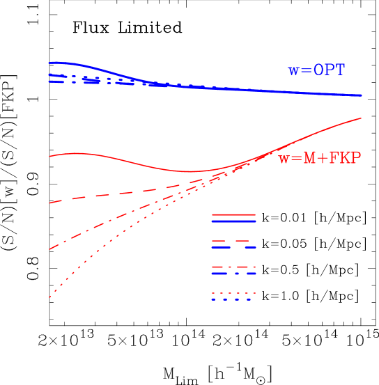
Figure 2: Same as Figure 1 except this time for a flux-limited survey.

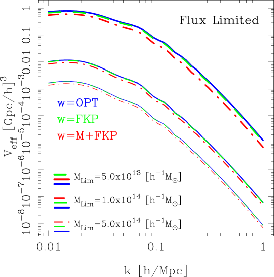
Figure 3: Effective survey volume as a function of the power spectrum wavenumber probed. Lines of decreasing thickness correspond to a minimum detectable mass $M_{\rm Lim}(0)$, of $5.0\times 10^{13}h^{-1}M_{\odot}$, $1.0\times 10^{14}h^{-1}M_{\odot}$, $5.0\times 10^{14}h^{-1}M_{\odot}$, respectively. The solid, dashed and dot-dashed lines correspond to $V_{\rm eff}$ for optimal, FKP and M+FKP weighting, respectively.

6.3 The Fisher matrix

As a final corollary to this section, we explore the cosmological information content of an optimally weighted cluster power spectrum analysis. Following Tegmark (1997), the Fisher information matrix for a power spectrum analysis can be defined as:

$${\mathcal{F}}_{\alpha\beta}=\sum_{i,j}\frac{\partial\overline{P}_{i}}{\partial\alpha}C^{-1}_{ij}\frac{\partial\overline{P}_{j}}{\partial\beta}=\sum_{i,j}\frac{\partial\log\overline{P}_{i}}{\partial\alpha}\overline{P}_{i}C^{-1}_{ij}\overline{P}_{j}\frac{\partial\log\overline{P}_{j}}{\partial\beta}\ ,$$ (66)

where $\partial/\partial\alpha\equiv\partial/\partial\theta_{\alpha}$ denote partial derivatives with respect to the cosmological parameters $\theta_{\alpha}$, and where here we have neglected the information content in the covariance matrix (Tegmark et al., 1997). On inserting our earlier expression for the covariance matrix, as given by Eq. (41), into the above expression, then the Fisher matrix becomes:

$${\mathcal{F}}_{\alpha\beta}=\sum_{i,j}\frac{\partial\log\overline{P}_{i}}{\partial\alpha}\overline{P}_{i}\frac{\delta^{K}_{ij}}{\sigma^{2}_{P}(k_{i})}\overline{P}_{j}\frac{\partial\log\overline{P}_{j}}{\partial\beta}=\sum_{i}\frac{\partial\log\overline{P}_{i}}{\partial\alpha}\frac{\partial\log\overline{P}_{i}}{\partial\beta}\left(\frac{{\mathcal{S}}}{{\mathcal{N}}}\right)_{\rm OPT}^{2}\!\!(k_{i})\ .$$ (67)

On inserting our expression for the ${\mathcal{S}}/{\mathcal{N}}$ for the optimal weights given by Eq. (58), the Fisher matrix, in the continuum limit of Fourier modes, can be written:

$${\mathcal{F}}_{\alpha\beta}=\frac{1}{2}\int\frac{{\rm d}{\bf k}}{(2\pi)^{3}}\frac{\partial\log P(k)}{\partial\alpha}\frac{\partial\log P(k)}{\partial\beta}V_{\rm eff}(k)\ ,$$ (68)

where the effective survey volume has the new form:

$$V_{\rm eff}(k)=\int_{0}^{\infty}d\chi\chi^{2}\left[\frac{\bar{n}_{\rm h}(\chi)\overline{b^{2}}(\chi)P(k)}{(1+\alpha)+\bar{n}_{\rm h}(\chi)\overline{b^{2}}(\chi)P(k)}\right]^{2}\ .$$ (69)

In Figure 3 we show the effective survey volume as a function of wavenumber, for a flux-limited survey of similar type to that described in §6.2. Here we consider the three cases where the minimum detectable mass normalization parameter from, c.f. Eq. (65), has the values $5.0\times 10^{13}h^{-1}M_{\odot}$, $1.0\times 10^{14}h^{-1}M_{\odot}$, $5.0\times 10^{14}h^{-1}M_{\odot}$, respectively. In all cases the optimal weighting increases $V_{\rm eff}$. Thus we conclude that the cosmological information extractable from an optimal weighted cluster survey will exceed that from the sub-optimal strategies, such as FKP or M+FKP weighting. Eq. (68) may thus be used as the starting point for exploring the cosmological information content of optimally weighted cluster power spectra (for a review of the Fisher matrix approach, see Heavens, 2009).

7 Conclusions

In this paper we have developed a formalism to compute weights maximizing the ${\mathcal{S}}/{\mathcal{N}}$ when estimating the cluster power spectrum, and used it to make inferences about the information in the matter power spectrum. Our derivation generalizes the original approach of FKP for galaxies, and is analogous to the derivation by PVP for examining the impact of luminosity dependent galaxy bias on the weights. Our derivation provides for the first time a completely analytic proof for the optimal weight equation, and it also corrects several errors that were found in these earlier works.

In §2 we described the generic properties of a cluster survey, taking into account finite survey geometry, arbitrary weighting of position and mass, and a flux limit; we also introduced out statistical treatment for describing the cluster density field using delta function expansions.

In §3 we presented estimators for recovering the matter clustering from the computation of the two-point correlation function and the power spectrum of the cluster field. We demonstrated that in order to extract information from the matter clustering one must deconvolve the survey window function. For large homogeneous survey volumes, provided an appropriate choice for the normalization of the cluster field is taken, this estimate was shown to be an unbiased estimator of the dark matter power spectrum, modulo a shot-noise correction.

In §4 we explored the statistical fluctuations in the power spectrum of clusters. We derived general expressions for the covariance of the cluster sample, including all non-Gaussian terms arising from the nonlinear evolution of matter fluctuations and discreteness effects. This generalized the result of Smith (2009). We then proved the necessary conditions for the covariance matrix to be diagonal.

In §5 we have provided an analytic derivation of the optimal weights for a cluster power spectrum analysis. We show in general terms that the optimal weights are separable functions of mass and space.

In §6 we presented a comparison of the optimal weighting scheme with the original FKP scheme and with a mass-weighting scheme. The latter was advocated by Seljak et al. (2009), later as a linear function of mass by Hamaus et al. (2010), in the context of reducing stochasticity in halo fields. In the limit of a low-mass cluster detection threshold the study of Cai et al. (2011) also found mass weighting to be optimal for matter density field reconstruction. For the case of both volume- and flux-limited cluster surveys the optimal weighting scheme outperforms both alternate weighting schemes. The gains over the FKP method are very modest $\sim 5\%$. Mass weighting performs significantly worse than the optimal scheme, with a relative loss in ${\mathcal{S}}/{\mathcal{N}}$ of $\sim 10\%$ on large scales, and of $\sim 20\%$ on intermediate scales. Whilst the mass-dependent weighting may be useful for reconstructing the matter field from a cluster sample, we recommend that it should not be used to extract cosmological information from cluster power spectrum analysis. We also presented a new expression for the Fisher information matrix, for an optimally-weighted cluster power spectrum measurement.

In this paper we have derived the optimal weights for measuring the cluster power spectrum under certain conditions, if these conditions are relaxed then the weights are no longer optimal. It will be interesting in future work to explore whether a more general weighting scheme can be derived for the more realistic situations where a non-diagonal covariance matrix is considered. We also expect that the weights that we have derived for the power spectrum should also be used to obtain optimal measurements of the cluster correlation function. However, we have not yet demonstrated this explicitly.

Appendix A Computing the 2-point correlations

Throughout this section we shall use the shorthand notation $\langle n_{\rm c}n^{\prime}_{\rm c}\rangle\equiv\langle n_{\rm c}({\bf x},M)n_{\rm c}({\bf x}^{\prime},M^{\prime})\rangle$, and similar for $\langle n_{\rm c}n^{\prime}_{s}\rangle,\,\langle n_{s}n^{\prime}_{s}\rangle$. The evaluation of these terms follows closely that of $<{\mathcal{F}}_{\rm c}>$. Proceeding with the first term, we write:

$$\left<n_{\rm c}n^{\prime}_{\rm c}\right>=\int\prod_{l=1}^{N}\left\{{\rm d}{\bf x}_{l}{\rm d}M_{l}\right\}p({\bf x}_{1},\dots,{\bf x}_{N},M_{1},\dots,M_{N})\sum_{i,j}^{N}\delta^{\rm D}({\bf x}-{\bf x}_{i})\delta^{\rm D}(M-M_{i})\delta^{\rm D}({\bf x}^{\prime}-{\bf x}_{j})\delta^{\rm D}(M^{\prime}-M_{j})\ .$$

The double sum can be broken up into the terms where $(i\neq j)$ and the terms where $(i=j)$, whereupon

$$\left<n_{\rm c}n^{\prime}_{\rm c}\right> = \int\prod_{l=1}^{N}\left\{{\rm d}{\bf x}_{l}{\rm d}M_{l}\right\}p({\bf x}_{1},\dots,{\bf x}_{N},M_{1},\dots,M_{N})\left[\sum_{i\neq j}^{N}\delta^{\rm D}({\bf x}-{\bf x}_{i})\delta^{\rm D}(M-M_{i})\delta^{\rm D}({\bf x}^{\prime}-{\bf x}_{j})\delta^{\rm D}(M^{\prime}-M_{j})\right.$$ (70)

$$+\left.\sum_{i=j}^{N}\delta^{\rm D}({\bf x}-{\bf x}_{i})\delta^{\rm D}({\bf x}^{\prime}-{\bf x}_{i})\delta^{\rm D}(M-M_{i})\delta^{\rm D}(M^{\prime}-M_{i})\right]$$

$$= \sum_{i\neq j}^{N}p({\bf x},{\bf x}^{\prime},M,M^{\prime})+\sum_{i=j}^{N}p({\bf x},M)\delta^{\rm D}({\bf x}-{\bf x}^{\prime})\delta^{\rm D}(M-M^{\prime})\ .$$

In order to proceed further, we need to specify the joint probability density distribution for obtaining clusters at positions ${\bf x}$ and ${\bf x}^{\prime}$ and with masses $M$ and $M^{\prime}$. This we do through the introduction of correlation functions:

$$p({\bf x},{\bf x}^{\prime},M,M^{\prime})\equiv p({\bf x},M)p({\bf x}^{\prime},M^{\prime})\left[1+\xi^{{\rm c}}({\bf x},{\bf x}^{\prime},M,M^{\prime})\right]=\frac{\bar{n}(M)\bar{n}(M^{\prime})}{N^{2}}\left[1+\xi^{{\rm c}}({\bf x},{\bf x}^{\prime},M,M^{\prime})\right]\ ,$$

where $\xi^{\rm c}({\bf x},{\bf x}^{\prime},M,M^{\prime})$ is the two-point cross-correlation function of clusters with masses $M$ and $M^{\prime}$. On use of the above definition in Eq. (70), we find

$$\left<n_{\rm c}n^{\prime}_{\rm c}\right>\approx\frac{}{}\bar{n}(M)\bar{n}(M^{\prime})\left[1+\xi^{\rm c}({\bf x},{\bf x}^{\prime},M,M^{\prime})\right]+\bar{n}(M)\delta^{\rm D}({\bf x}-{\bf x}^{\prime})\delta^{\rm D}(M-M^{\prime})\ ,$$ (71)

where in arriving at the last equality we have assumed that $N\gg 1$ and therefore $N-1\approx N$. We may now write down directly the remaining expectation values that enter Eq. (16), whereupon:

$$\left<n_{\rm c}n^{\prime}_{s}\right> = \alpha^{-1}\bar{n}(M)\bar{n}(M^{\prime})\ ;$$

$$\langle n_{s}n^{\prime}_{s}\rangle = \alpha^{-2}\bar{n}(M)\bar{n}(M^{\prime})+\alpha^{-1}\bar{n}(M)\delta^{\rm D}({\bf x}-{\bf x}^{\prime})\delta^{\rm D}(M-M^{\prime})\ .$$ (72)

Appendix B Statistical fluctuations in the ${\mathcal{F}}_{\rm c}$ power spectrum

B.1 General expression of the covariance of the power spectrum estimator

The covariance of the matter power spectrum estimator given by Eq. (31) is formed of four terms:

$${\rm Cov}\!\left[\hat{P}({\bf k}_{1}),\hat{P}({\bf k}_{2})\right]={\rm Cov}\!\left[|\widetilde{\mathcal{F}}_{\rm c}({\bf k}_{1})|^{2},|\widetilde{\mathcal{F}}_{\rm c}({\bf k}_{2})|^{2}\right]+{\rm Var}\!\left[P_{\rm shot}\right]-{\rm Cov}\!\left[|\widetilde{\mathcal{F}}_{\rm c}({\bf k}_{1})|^{2},P_{\rm shot}\right]-{\rm Cov}\!\left[|\widetilde{\mathcal{F}}_{\rm c}({\bf k}_{2})|^{2},P_{\rm shot}\right]\ ,$$ (73)

where

$${\rm Cov}\!\left[|\widetilde{\mathcal{F}}_{\rm c}({\bf k}_{1})|^{2},|\widetilde{\mathcal{F}}_{\rm c}({\bf k}_{2})|^{2}\right] \equiv \left<|\widetilde{\mathcal{F}}_{\rm c}({\bf k}_{1})|^{2}|\widetilde{\mathcal{F}}_{\rm c}({\bf k}_{2})|^{2}\right>-\left<|\widetilde{\mathcal{F}}_{\rm c}({\bf k}_{1})|^{2}\right>\left<|\widetilde{\mathcal{F}}_{\rm c}({\bf k}_{2})|^{2}\right>\ ;$$

$${\rm Var}\!\left[P_{\rm shot}\right] \equiv \left<[P_{\rm shot}]^{2}\right>-\left<P_{\rm shot}\right>^{2}\ ;$$

$${\rm Cov}\!\left[|\widetilde{\mathcal{F}}_{\rm c}({\bf k}_{i})|^{2},P_{\rm shot}\right] \equiv \left<|\widetilde{\mathcal{F}}_{\rm c}({\bf k}_{i})|^{2}P_{\rm shot}\right>-\left<|\widetilde{\mathcal{F}}_{\rm c}({\bf k}_{i})|^{2}\right>\left<P_{\rm shot}\right>\ \ \ ;\ \ i\in(1,2)\ .$$ (74)

Assuming that the total number density of clusters is a deterministic quantity, all of the covariance terms involving $P_{\rm shot}$ vanish. Thus we are left with the task of determining the covariance of the modulus square of the $\widetilde{\mathcal{F}}_{\rm c}$ field, i.e. Eq. (33).

B.2 Derivation of the covariance of the power spectrum estimator

For a succint presentation of the covariance calculation, we make use of the following shorthand notation:

$$\bar{n}_{i}\equiv\bar{n}(M_{i})\>;\>\>w_{i}\equiv w({\bf x}_{i},M_{i})\>;\>\>b_{i}\equiv b(M_{i})\>;\>\>\Theta_{i}\equiv\Theta({\bf x}_{i}|M_{i})\>;\>\>n_{{\rm c},i}\equiv n_{\rm c}({\bf x}_{i},M_{i})\>;\>\>n_{s,i}\equiv n_{s}({\bf x}_{i},M_{i})\>;\>\>\delta^{\rm D}_{ij}\equiv\delta^{\rm D}({\bf x}_{i}-{\bf x}_{j})\delta^{\rm D}(M_{i}-M_{j})\ .$$ (75)

The covariance matrix of the power in the field ${\mathcal{F}}_{\rm c}$ can be written:

$${\rm Cov}\!\left[|\widetilde{\mathcal{F}}_{\rm c}({\bf k}_{1})|^{2},|\widetilde{\mathcal{F}}_{\rm c}({\bf k}_{2})|^{2}\right]=\int{\rm d}{\bf k}_{3}\,{\rm d}{\bf k}_{4}\delta^{\rm D}({\bf k}_{1}+{\bf k}_{3})\delta^{\rm D}({\bf k}_{2}+{\bf k}_{4})\left[\left<\widetilde{\mathcal{F}}_{\rm c}({\bf k}_{1})\dots\widetilde{\mathcal{F}}_{\rm c}({\bf k}_{4})\right>-\left<\widetilde{\mathcal{F}}_{\rm c}({\bf k}_{1})\widetilde{\mathcal{F}}_{\rm c}({\bf k}_{3})\right>\left<\widetilde{\mathcal{F}}_{\rm c}({\bf k}_{2})\widetilde{\mathcal{F}}_{\rm c}({\bf k}_{4})\right>\right]$$ (76)

In order to proceed further we see that we must compute the four-point correlation function of the Fourier modes $\widetilde{\mathcal{F}}_{\rm c}({\bf k})$. This is equivalent to specifying the four-point correlation function of the field ${\mathcal{F}}_{\rm c}$:

$$\left<\widetilde{\mathcal{F}}_{\rm c}({\bf k}_{1})\dots\widetilde{\mathcal{F}}_{\rm c}({\bf k}_{4})\right>=\int{\rm d}{\bf x}_{1}\dots\rm d{\bf x}_{4}\left<{\mathcal{F}}_{\rm c}({\bf x}_{1})\dots\mathcal{F}_{\rm c}({\bf x}_{4})\right>{\rm e}^{i{\bf k}_{1}\cdot{\bf x}_{1}+\dots+{\bf k}_{4}\cdot{\bf x}_{4}}\ .$$ (77)

Substituting Eq. (9) into the expression for the four-point correlation function, we find:

$$\left<{\mathcal{F}}_{\rm c}({\bf x}_{1})\dots\mathcal{F}_{\rm c}({\bf x}_{4})\right>=\frac{1}{A^{2}}\int\prod_{i=1}^{4}\left\{{\rm d}M_{i}w({\bf x}_{i},M_{i})\Theta({\bf x}_{i}|M_{i})\right\}\left<\frac{}{}\left[n_{\rm c}({\bf x}_{1},M_{1})-\alpha n_{s}({\bf x}_{1},M_{1})\right]\dots\left[n_{\rm c}({\bf x}_{4},M_{4})-\alpha n_{s}({\bf x}_{4})\right]\right>\ .$$ (78)

Expanding the term in angled braces on the right-hand side gives,

$$\left<\left[n_{{\rm c},1}-\alpha n_{s,1}\right]\dots\left[n_{{\rm c},4}-\alpha n_{s,4}\right]\right> = \left<n_{{\rm c},1}\dots n_{{\rm c},4}\right>-\alpha\left[\frac{}{}\left<n_{{\rm c},1}n_{{\rm c},2}n_{{\rm c},3}n_{s,4}\right>+{3\rm cyc}\right]+\alpha^{2}\left[\frac{}{}\left<n_{{\rm c},1}n_{{\rm c},2}n_{s,3}n_{s,4}\right>+{5\rm perm}\right]$$ (79)

$$-\alpha^{3}\left[\frac{}{}\left<n_{{\rm c},1}n_{s,2}n_{s,3}n_{s,4}\right>+{3\rm cyc}\right]+\frac{}{}\alpha^{4}\left<n_{s,1}\dots n_{s,4}\right>\ .$$

We focus on the first term in curly brackets on the right-hand side, and insert our delta function expansion for the number density field:

$$\left<n_{{\rm c},1}\dots n_{{\rm c},4}\right> = \left<\sum_{i_{1},i_{2},i_{3},i_{4}=1}^{N}\delta^{\rm D}({\bf x}_{1}-{\bf x}^{\prime}_{i_{1}})\dots\delta^{\rm D}({\bf x}_{4}-{\bf x}^{\prime}_{i_{4}})\delta^{\rm D}(M_{1}-M^{\prime}_{i_{1}})\dots\delta^{\rm D}(M_{4}-M^{\prime}_{i_{4}})\right>$$ (80)

$$= \int\prod_{p=1}^{N}\left\{{\rm d}{\bf x}^{\prime}_{p}\,{\rm d}M^{\prime}_{p}\right\}p({\bf x}^{\prime}_{1},\dots,{\bf x}^{\prime}_{N},M^{\prime}_{1},\dots,M^{\prime}_{N})\left\{\Gamma_{1}+\Gamma_{2}+\Gamma_{3}+\Gamma_{4}+\Gamma_{5}\right\}\ ,$$

where in the above we have defined the following terms:

$$\Gamma_{1} \equiv \sum_{i_{1}\neq i_{2}\neq i_{3}\neq i_{4}}\delta^{\rm D}({\bf x}_{1}-{\bf x}^{\prime}_{i_{1}})\dots\delta^{\rm D}({\bf x}_{4}-{\bf x}^{\prime}_{i_{4}})\delta^{\rm D}(M_{1}-M^{\prime}_{i_{1}})\dots\delta^{\rm D}(M_{4}-M^{\prime}_{i_{4}})\ ;$$

$$\Gamma_{2} \equiv \sum_{i_{1}\neq i_{2}\neq i_{3}=i_{4}}\delta^{\rm D}({\bf x}_{1}-{\bf x}^{\prime}_{i_{1}})\delta^{\rm D}({\bf x}_{2}-{\bf x}^{\prime}_{i_{2}})\delta^{\rm D}(M_{1}-M^{\prime}_{i_{1}})\delta^{\rm D}(M_{2}-M_{i_{2}})\prod_{p=3}^{4}\left\{\delta^{\rm D}({\bf x}_{p}-{\bf x}^{\prime}_{i_{3}})\delta^{\rm D}(M_{p}-M^{\prime}_{i_{3}})\right\}+5{\rm perms}\ ;$$

$$\Gamma_{3} \equiv \sum_{i_{1}=i_{2}\neq i_{3}=i_{4}}\prod_{p=1}^{2}\left\{\delta^{\rm D}({\bf x}_{p}-{\bf x}^{\prime}_{i_{1}})\delta^{\rm D}(M_{p}-M^{\prime}_{i_{1}})\right\}\prod_{q=3}^{4}\left\{\delta^{\rm D}({\bf x}_{q}-{\bf x}^{\prime}_{i_{3}}\delta^{\rm D}(M_{q}-M^{\prime}_{i_{3}})\right\}+2{\rm perms}\ ;$$

$$\Gamma_{4} \equiv \sum_{i_{1}\neq i_{2}=i_{3}=i_{4}}\delta^{\rm D}({\bf x}_{1}-{\bf x}^{\prime}_{i_{1}})\delta^{\rm D}(M_{1}-M^{\prime}_{i_{1}})\prod_{p=2}^{4}\left\{\delta^{\rm D}({\bf x}_{p}-{\bf x}^{\prime}_{i_{2}})\delta^{\rm D}(M_{p}-M^{\prime}_{i_{2}})\right\}+3{\rm perms}\ ;$$

$$\Gamma_{5} \equiv \sum_{i_{1}=i_{2}=i_{3}=i_{4}}\prod_{p=1}^{4}\left\{\delta^{\rm D}({\bf x}_{p}-{\bf x}^{\prime}_{i_{1}})\delta^{\rm D}(M_{p}-M^{\prime}_{i_{1}})\right\}\ .$$ (81)

We now compute the contributions from each of the five $\Gamma$ terms.

$\bullet$ Computing $\langle\Gamma_{1}\rangle$ : On performing the integrations over the delta functions we have:

$$\langle\Gamma_{1}\rangle = \sum_{i_{1}\neq i_{2}\neq i_{3}\neq i_{4}}p({\bf x}_{1},\dots,{\bf x}_{4},M_{1},\dots,M_{4})$$ (82)

$$= N(N-1)(N-2)(N-3)p({\bf x}_{1},M_{1})\dots p({\bf x}_{4},M_{4})\left[\frac{}{}1+\xi^{\rm c}_{12}+\xi^{\rm c}_{13}+\xi^{\rm c}_{14}+\xi^{\rm c}_{23}+\xi^{\rm c}_{24}+\xi^{\rm c}_{34}\right.$$

$$\left.\frac{}{}+\zeta^{\rm c}_{123}+\zeta^{\rm c}_{234}+\zeta^{\rm c}_{341}+\zeta^{\rm c}_{412}+\xi^{\rm c}_{12}\xi^{\rm c}_{34}+\xi^{\rm c}_{13}\xi^{\rm c}_{24}+\xi^{\rm c}_{14}\xi^{\rm c}_{23}+\eta^{\rm c}_{1234}\right]$$

$$\approx \prod_{p=1}^{4}\left\{\bar{n}_{p}\right\}\left[\frac{}{}1+\xi^{\rm c}_{12}+\xi^{\rm c}_{13}+\xi^{\rm c}_{14}+\xi^{\rm c}_{23}+\xi^{\rm c}_{24}+\xi^{\rm c}_{34}+\zeta^{\rm c}_{123}+\zeta^{\rm c}_{234}+\zeta^{\rm c}_{341}+\zeta^{\rm c}_{412}+\xi^{\rm c}_{12}\xi^{\rm c}_{34}+\xi^{\rm c}_{13}\xi^{\rm c}_{24}+\xi^{\rm c}_{14}\xi^{\rm c}_{23}+\eta^{\rm c}_{1234}\right],\hskip 28.45274pt$$

where the last equality holds in the limit that $N\gg 1$. The terms $\zeta^{\rm c}$ and $\eta^{\rm c}$ are the three- and four-point correlation functions of the haloes, respectively, and in the above we have also made use of the short-hand notation:

$$\xi^{\rm c}_{ij}\equiv\xi^{\rm c}({\bf r}_{i},{\bf r}_{j},M_{i},M_{j})\hskip 8.5359pt;\hskip 8.5359pt\zeta^{\rm c}_{ijk}\equiv\zeta({\bf r}_{i},{\bf r}_{j},{\bf r}_{k},M_{i},M_{j},M_{k})\hskip 8.5359pt;\hskip 8.5359pt\eta^{\rm c}_{ijkl}\equiv\eta^{\rm c}({\bf r}_{i},{\bf r}_{j},{\bf r}_{k},{\bf r}_{l},M_{i},M_{j},M_{k},M_{l})\hskip 8.5359pt.$$ (83)

$\bullet$ Computing $\langle\Gamma_{2}\rangle$ : On integration over the delta functions and using Eq. (75), we obtain:

$$\langle\Gamma_{2}\rangle \equiv \sum_{i_{1}\neq i_{2}\neq i_{3}=i_{4}}p({\bf x}_{1},{\bf x}_{2},{\bf x}_{3},M_{1},M_{2},M_{3})\,\delta^{\rm D}_{34}+\sum_{i_{1}\neq i_{2}=i_{3}\neq i_{4}}p({\bf x}_{1},{\bf x}_{2},{\bf x}_{4},M_{1},M_{2},M_{4})\,\delta^{\rm D}_{23}+\sum_{i_{1}=i_{2}\neq i_{3}\neq i_{4}}p({\bf x}_{1},{\bf x}_{3},{\bf x}_{4},M_{1},M_{3},M_{4})\,\delta^{\rm D}_{12}$$

$$+\sum_{i_{1}=i_{3}\neq i_{2}\neq i_{4}}p({\bf x}_{1},{\bf x}_{2},{\bf x}_{4},M_{1},M_{2},M_{4})\,\delta^{\rm D}_{13}+\sum_{i_{1}=i_{4}\neq i_{2}\neq i_{3}}p({\bf x}_{1},{\bf x}_{2},{\bf x}_{3},M_{1},M_{2},M_{3})\,\delta^{\rm D}_{14}+\sum_{i_{2}=i_{4}\neq i_{1}\neq i_{3}}p({\bf x}_{1},{\bf x}_{2},{\bf x}_{3},M_{1},M_{2},M_{3})\,\delta^{\rm D}_{24}\ .$$

On performing the summations and taking the limit of large numbers, the above expression reduces to:

$$\langle\Gamma_{2}\rangle = \prod_{p\in\{1,3,4\}}\{\bar{n}_{p}\}[1+\xi^{\rm c}_{13}+\xi^{\rm c}_{14}+\xi^{\rm c}_{34}+\zeta^{\rm c}_{134}]\delta^{\rm D}_{12}+\prod_{p\in\{1,2,4\}}\{\bar{n}_{p}\}[1+\xi^{\rm c}_{12}+\xi^{\rm c}_{24}+\xi^{\rm c}_{24}+\zeta^{\rm c}_{124}]\delta^{\rm D}_{23}+\prod_{p\in\{1,2,3\}}\{\bar{n}_{p}\}[1+\xi^{\rm c}_{12}+\xi^{\rm c}_{13}+\xi^{\rm c}_{23}+\zeta^{\rm c}_{123}]\delta^{\rm D}_{14}$$

$$+\prod_{p\in\{1,2,4\}}\{\bar{n}_{p}\}[1+\xi^{\rm c}_{12}+\xi^{\rm c}_{14}+\xi^{\rm c}_{24}+\zeta^{\rm c}_{124}]\delta^{\rm D}_{23}+\prod_{p\in\{1,2,3\}}\{\bar{n}_{p}\}[1+\xi^{\rm c}_{12}+\xi^{\rm c}_{23}+\xi^{\rm c}_{31}+\zeta^{\rm c}_{123}]\delta^{\rm D}_{24}+\prod_{p\in\{1,2,3\}}\{\bar{n}_{p}\}[1+\xi^{\rm c}_{12}+\xi^{\rm c}_{23}+\xi^{\rm c}_{31}+\zeta^{\rm c}_{123}]\delta^{\rm D}_{34}\ .$$

$\bullet$ Computing $\langle\Gamma_{3}\rangle$ : On performing the integrations over the delta functions, we have:

$$\langle\Gamma_{3}\rangle \equiv \sum_{i_{1}=i_{2}\neq i_{3}=i_{4}}p({\bf x}_{1},{\bf x}_{3},M_{1},M_{3})\delta^{\rm D}_{12}\delta^{\rm D}_{34}+\sum_{i_{1}=i_{3}\neq i_{2}=i_{4}}p({\bf x}_{1},{\bf x}_{2},M_{1},M_{2})\delta^{\rm D}_{13}\delta^{\rm D}_{24}+\sum_{i_{1}=i_{4}\neq i_{2}=i_{3}}p({\bf x}_{1},{\bf x}_{2},M_{1},M_{2})\delta^{\rm D}_{14}\delta^{\rm D}_{23}$$ (85)

$$= \frac{}{}\bar{n}_{1}\bar{n}_{3}\left[1+\xi^{\rm c}_{13}\right]\delta^{\rm D}_{12}\delta^{\rm D}_{34}+\bar{n}_{1}\bar{n}_{2}\left[1+\xi^{\rm c}_{12}\right]\left[\frac{}{}\delta^{\rm D}_{13}\delta^{\rm D}_{24}+\delta^{\rm D}_{14}\delta^{\rm D}_{23}\right]\ ,$$

where to arrive at the second equality, we performed the summations in the limit of a large number of clusters.

$\bullet$ Computing $\langle\Gamma_{4}\rangle$ : We perform the integrations over the delta functions to obtain:

$$\langle\Gamma_{4}\rangle \equiv \sum_{i_{1}=i_{2}=i_{3}\neq i_{4}}p({\bf x}_{1},{\bf x}_{4},M_{1},M_{4})\delta^{\rm D}_{12}\delta^{\rm D}_{13}+\sum_{i_{1}=i_{2}=i_{4}\neq i_{3}}p({\bf x}_{1},{\bf x}_{3},M_{1},M_{3})\delta^{\rm D}_{12}\delta^{\rm D}_{14}+\sum_{i_{1}=i_{3}=i_{4}\neq i_{2}}p({\bf x}_{1},{\bf x}_{2},M_{1},M_{2})\delta^{\rm D}_{13}\delta^{\rm D}_{14}+\sum_{i_{2}=i_{3}=i_{4}\neq i_{1}}p({\bf x}_{1},{\bf x}_{2},M_{1},M_{2})\delta^{\rm D}_{23}\delta^{\rm D}_{24}\ .$$

Summing and taking the limit of large numbers of clusters we find:

$$\langle\Gamma_{4}\rangle = \bar{n}_{1}\bar{n}_{4}\left[1+\xi^{\rm c}_{14}\right]\delta^{\rm D}_{12}\delta^{\rm D}_{13}+\bar{n}_{1}\bar{n}_{3}\left[1+\xi^{\rm c}_{13}\right]\delta^{\rm D}_{12}\delta^{\rm D}_{14}+\bar{n}_{1}\bar{n}_{2}\left[1+\xi^{\rm c}_{12}\right]\left\{\delta^{\rm D}_{13}\delta^{\rm D}_{14}+\delta^{\rm D}_{23}\delta^{\rm D}_{24}\right\}\ .$$ (86)

$\bullet$ Computing $\langle\Gamma_{5}\rangle$ : Integrating over the delta functions leads to:

$$\langle\Gamma_{5}\rangle \equiv \sum_{i_{1}=i_{2}=i_{3}=i_{4}}p({\bf x}_{1},M_{1})\delta^{\rm D}_{12}\delta^{\rm D}_{13}\delta^{\rm D}_{14}=\frac{}{}\bar{n}_{1}\delta^{\rm D}_{12}\delta^{\rm D}_{13}\delta^{\rm D}_{14}\ .$$ (87)

Putting together the terms Eqs. 82–87 we arrive at the expression:

$$\left<n_{{\rm c},1}\dots n_{{\rm c},4}\right> = \prod_{p=1}^{4}\{\bar{n}_{p}\}\left\{\frac{}{}\left[\frac{}{}1+\xi^{\rm c}_{12}+\xi^{\rm c}_{13}+\xi^{\rm c}_{14}+\xi^{\rm c}_{23}+\xi^{\rm c}_{24}+\xi^{\rm c}_{34}+\zeta^{\rm c}_{123}+\zeta^{\rm c}_{234}+\zeta^{\rm c}_{341}+\zeta^{\rm c}_{412}+\xi^{\rm c}_{12}\xi^{\rm c}_{34}+\xi^{\rm c}_{13}\xi^{\rm c}_{24}+\xi^{\rm c}_{14}\xi^{\rm c}_{23}+\eta^{\rm c}_{1234}\right]\right.$$ (88)

$$\left.+\left[\frac{}{}1+\xi^{\rm c}_{13}+\xi^{\rm c}_{14}+\xi^{\rm c}_{34}+\zeta^{\rm c}_{134}\right]\frac{\delta^{\rm D}_{12}}{\bar{n}_{2}}+\left[\frac{}{}1+\xi^{\rm c}_{12}+\xi^{\rm c}_{24}+\xi^{\rm c}_{41}+\zeta^{\rm c}_{124}\right]\frac{\delta^{\rm D}_{23}}{\bar{n}_{3}}+\left[\frac{}{}1+\xi^{\rm c}_{12}+\xi^{\rm c}_{13}+\xi^{\rm c}_{23}+\zeta^{\rm c}_{123}\right]\frac{\delta^{\rm D}_{14}}{\bar{n}_{4}}\right.$$

$$\left.+\left[\frac{}{}1+\xi^{\rm c}_{12}+\xi^{\rm c}_{14}+\xi^{\rm c}_{24}+\zeta^{\rm c}_{124}\right]\frac{\delta^{\rm D}_{13}}{\bar{n}_{3}}+\left[\frac{}{}1+\xi^{\rm c}_{12}+\xi^{\rm c}_{23}+\xi^{\rm c}_{31}+\zeta^{\rm c}_{123}\right]\frac{\delta^{\rm D}_{r,24}}{\bar{n}_{4}}+\left[\frac{}{}1+\xi^{\rm c}_{12}+\xi^{\rm c}_{23}+\xi^{\rm c}_{31}+\zeta^{\rm c}_{123}\right]\frac{\delta^{\rm D}_{34}}{\bar{n}_{4}}\right.$$

$$\left.+\left[\frac{}{}1+\xi^{\rm c}_{13}\right]\frac{\delta^{\rm D}_{12}\delta^{\rm D}_{34}}{\bar{n}_{2}\bar{n}_{4}}+\left[\frac{}{}1+\xi^{\rm c}_{12}\right]\frac{\delta^{\rm D}_{13}\delta^{\rm D}_{24}}{\bar{n}_{3}\bar{n}_{4}}+\left[\frac{}{}1+\xi^{\rm c}_{12}\right]\frac{\delta^{\rm D}_{14}\delta^{\rm D}_{23}}{\bar{n}_{3}\bar{n}_{4}}+\left[\frac{}{}1+\xi^{\rm c}_{14}\right]\frac{\delta^{\rm D}_{12}\delta^{\rm D}_{13}}{\bar{n}_{2}\bar{n}_{3}}\right.$$

$$\left.+\left[\frac{}{}1+\xi^{\rm c}_{13}\right]\frac{\delta^{\rm D}_{12}\delta^{\rm D}_{14}}{\bar{n}_{2}\bar{n}_{4}}+\left[\frac{}{}1+\xi^{\rm c}_{12}\right]\frac{\delta^{\rm D}_{13}\delta^{\rm D}_{14}+\delta^{\rm D}_{23}\delta^{\rm D}_{24}}{\bar{n}_{3}\bar{n}_{4}}+\frac{\delta^{\rm D}_{12}\delta^{\rm D}_{13}\delta^{\rm D}_{14}}{\bar{n}_{2}\bar{n}_{3}\bar{n}_{3}}\right\}\ .$$

In the above $\xi^{{\rm c}}_{ij}$, $\zeta^{{\rm c}}_{ijk}$ and $\eta^{{\rm c}}_{ijkl}$ represent the true three- and four-point connected correlation functions of galaxy clusters, respectively. Under the assumption of linear biasing these may be written in terms of the connected correlation functions of the matter as:

$$\xi^{\rm c}_{ij} \equiv \xi_{{\rm c}}({\bf x}_{i},{\bf x}_{j},M_{i},M_{j})=b(M_{i})b(M_{j})\xi_{ij}=b_{i}b_{j}\xi_{ij}\ ;$$

$$\zeta^{\rm c}_{ijk} \equiv \zeta_{{\rm c}}({\bf x}_{i},{\bf x}_{j},{\bf x}_{k},M_{i},M_{j},M_{k})=b(M_{i})b(M_{j})b(M_{k})\zeta_{ijk}=b_{i}b_{j}b_{k}\zeta_{ijk}\ ;$$

$$\eta^{\rm c}_{1234} \equiv \eta_{{\rm c}}({\bf x}_{1},{\bf x}_{2},{\bf x}_{3},{\bf x}_{4},M_{1},M_{2},M_{3},M_{4})=b(M_{1})b(M_{2})b(M_{3})b(M_{4})\eta_{1234}=b_{1}b_{2}b_{3}b_{4}\eta_{1234}\ .$$

Similar to the result of Eq. (88), we can also write down the terms entering Eq. (79). Thus we obtain:

$$\left<n_{{\rm c},1}\,n_{{\rm c},2}\,n_{{\rm c},3}\,n_{s,4}\right> \equiv \alpha^{-1}\prod_{p=1}^{4}\{\bar{n}_{p}\}\left\{\left[\frac{}{}1+\xi^{\rm c}_{12}+\xi^{\rm c}_{13}+\xi^{\rm c}_{23}+\zeta^{\rm c}_{123}\right]+\left[\frac{}{}1+\xi^{\rm c}_{13}\right]\frac{\delta^{\rm D}_{12}}{\bar{n}_{2}}+\left[\frac{}{}1+\xi^{\rm c}_{12}\right]\frac{\delta^{\rm D}_{23}+\delta^{\rm D}_{13}}{\bar{n}_{3}}+\frac{\delta^{\rm D}_{12}\delta^{\rm D}_{13}}{\bar{n}_{2}\bar{n}_{3}}\right\}\ ;$$

$$\left<n_{{\rm c},1}\,n_{{\rm c},2}\,n_{s,3}\,n_{s,4}\right> \equiv \alpha^{-2}\prod_{p=1}^{4}\{\bar{n}_{p}\}\left\{\left[\frac{}{}1+\xi^{\rm c}_{12}\right]+\frac{\delta^{\rm D}_{12}}{\bar{n}_{2}}+\alpha\left[\frac{}{}1+\xi^{\rm c}_{12}\right]\frac{\delta^{\rm D}_{34}}{\bar{n}_{4}}+\alpha\frac{\delta^{\rm D}_{12}\delta^{\rm D}_{34}}{\bar{n}_{2}\bar{n}_{4}}\right\}\ ;$$

$$\left<n_{{\rm c},1}\,n_{s,2}\,n_{s,3}\,n_{s,4}\right> \equiv \alpha^{-3}\prod_{p=1}^{4}\{\bar{n}_{p}\}\left\{1+\alpha\left[\frac{\delta^{\rm D}_{23}}{\bar{n}_{3}}+\frac{\delta^{\rm D}_{24}}{\bar{n}_{4}}+\frac{\delta^{\rm D}_{34}}{\bar{n}_{4}}\right]+\alpha^{2}\frac{\delta^{\rm D}_{23}\delta^{\rm D}_{24}}{\bar{n}_{3}\bar{n}_{4}}\right\}\ ;$$

$$\left<n_{s,1}\,n_{s,2}\,n_{s,3}\,n_{s,4}\right> \equiv \alpha^{-4}\prod_{p=1}^{4}\{\bar{n}_{p}\}\left\{1+\alpha\left[\frac{\delta^{\rm D}_{12}}{\bar{n}_{2}}+\frac{\delta^{\rm D}_{13}+\delta^{\rm D}_{23}}{\bar{n}_{3}}+\frac{\delta^{\rm D}_{14}+\delta^{\rm D}_{24}+\delta^{\rm D}_{34}}{\bar{n}_{4}}\right]+\alpha^{2}\left[\frac{\delta^{\rm D}_{12}\delta^{\rm D}_{14}+\delta^{\rm D}_{12}\delta^{\rm D}_{34}}{\bar{n}_{2}\bar{n}_{4}}+\frac{\delta^{\rm D}_{12}\delta^{\rm D}_{13}}{\bar{n}_{2}\bar{n}_{3}}\right.\right.$$ (89)

$$+\left.\left.\frac{\delta^{\rm D}_{13}\delta^{\rm D}_{24}+\delta^{\rm D}_{14}\delta^{\rm D}_{23}+\delta^{\rm D}_{13}\delta^{\rm D}_{14}+\delta^{\rm D}_{23}\delta^{\rm D}_{24}}{\bar{n}_{3}\bar{n}_{4}}\right]+\frac{}{}\alpha^{3}\frac{\delta^{\rm D}_{12}\delta^{\rm D}_{13}\delta^{\rm D}_{14}}{\bar{n}_{2}\bar{n}_{3}\bar{n}_{4}}\right\}\ .$$

Hence, for the second term in Eq. (79) we have:

$$\left<n_{{\rm c},1}\,n_{{\rm c},2}\,n_{{\rm c},3}\,n_{s,4}\right>+{\rm 3perms} = \alpha^{-1}\prod_{p=1}^{4}\{\bar{n}_{p}\}\left[\frac{}{}4+2\left(\frac{}{}\xi^{\rm c}_{12}+\xi^{\rm c}_{13}+\xi^{\rm c}_{23}+\xi^{\rm c}_{14}+\xi^{\rm c}_{24}+\xi^{\rm c}_{34}\right)+\zeta^{\rm c}_{123}+\zeta^{\rm c}_{124}+\zeta^{\rm c}_{134}+\zeta^{\rm c}_{234}\right]$$ (90)

$$+\left[\frac{}{}1+\xi^{\rm c}_{13}\right]\frac{\delta^{\rm D}_{12}}{\bar{n}_{2}}+\left[\frac{}{}1+\xi^{\rm c}_{12}\right]\frac{\delta^{\rm D}_{23}}{\bar{n}_{3}}+\left[\frac{}{}1+\xi^{\rm c}_{12}\right]\frac{\delta^{\rm D}_{31}}{\bar{n}_{3}}+\left[\frac{}{}1+\xi^{\rm c}_{14}\right]\frac{\delta^{\rm D}_{12}}{\bar{n}_{2}}+\left[\frac{}{}1+\xi^{\rm c}_{12}\right]\frac{\delta^{\rm D}_{24}}{\bar{n}_{4}}$$

$$+\left[\frac{}{}1+\xi^{\rm c}_{12}\right]\frac{\delta^{\rm D}_{41}}{\bar{n}_{4}}+\left[\frac{}{}1+\xi^{\rm c}_{14}\right]\frac{\delta^{\rm D}_{13}}{\bar{n}_{3}}+\left[\frac{}{}1+\xi^{\rm c}_{13}\right]\frac{\delta^{\rm D}_{14}}{\bar{n}_{4}}+\left[\frac{}{}1+\xi^{\rm c}_{13}\right]\frac{\delta^{\rm D}_{34}}{\bar{n}_{4}}+\left[\frac{}{}1+\xi^{\rm c}_{24}\right]\frac{\delta^{\rm D}_{23}}{\bar{n}_{3}}$$

$$+\left[\frac{}{}1+\xi^{\rm c}_{23}\right]\frac{\delta^{\rm D}_{24}}{\bar{n}_{4}}+\left[\frac{}{}1+\xi^{\rm c}_{23}\right]\frac{\delta^{\rm D}_{34}}{\bar{n}_{4}}+\frac{\delta^{\rm D}_{12}\delta^{\rm D}_{13}}{\bar{n}_{2}\bar{n}_{3}}+\frac{\delta^{\rm D}_{12}\delta^{\rm D}_{14}}{\bar{n}_{2}\bar{n}_{4}}+\frac{\delta^{\rm D}_{13}\delta^{\rm D}_{14}+\delta^{\rm D}_{23}\delta^{\rm D}_{24}}{\bar{n}_{3}\bar{n}_{4}}\ .$$

For the third term in Eq. (79) we obtain:

$$\left<n_{{\rm c},1}\,n_{{\rm c},2}\,n_{s,3}\,n_{s,4}\right>+{\rm 5\ perms} = \alpha^{-2}\prod_{p=1}^{4}\{\bar{n}_{p}\}\left\{\left[\frac{}{}6+\xi^{\rm c}_{12}+\xi^{\rm c}_{13}+\xi^{\rm c}_{14}+\xi^{\rm c}_{23}+\xi^{\rm c}_{24}+\xi^{\rm c}_{34}\right]+\frac{\delta^{\rm D}_{12}}{\bar{n}_{2}}+\frac{\delta^{\rm D}_{13}+\delta^{\rm D}_{23}}{\bar{n}_{3}}+\frac{\delta^{\rm D}_{14}+\delta^{\rm D}_{24}+\delta^{\rm D}_{34}}{\bar{n}_{4}}\right.$$ (91)

$$\left.+\alpha\left\{\left[\frac{}{}1+\xi^{\rm c}_{12}\right]\frac{\delta^{\rm D}_{34}}{\bar{n}_{4}}+\left[\frac{}{}1+\xi^{\rm c}_{13}\right]\frac{\delta^{\rm D}_{24}}{\bar{n}_{4}}+\left[\frac{}{}1+\xi^{\rm c}_{23}\right]\frac{\delta^{\rm D}_{14}}{\bar{n}_{4}}+\left[\frac{}{}1+\xi^{\rm c}_{14}\right]\frac{\delta^{\rm D}_{23}}{\bar{n}_{3}}+\left[\frac{}{}1+\xi^{\rm c}_{24}\right]\frac{\delta^{\rm D}_{13}}{\bar{n}_{3}}\right.\right.$$

$$\left.\left.+\left[\frac{}{}1+\xi^{\rm c}_{34}\right]\frac{\delta^{\rm D}_{12}}{\bar{n}_{2}}+2\frac{\delta^{\rm D}_{12}\delta^{\rm D}_{34}}{\bar{n}_{2}\bar{n}_{4}}+2\frac{\delta^{\rm D}_{13}\delta^{\rm D}_{24}+\delta^{\rm D}_{14}\delta^{\rm D}_{23}}{\bar{n}_{3}\bar{n}_{4}}\right\}\right\}\ .$$

For the fourth term in Eq. (79), we write:

$$\left<n_{{\rm c},1}\,n_{s,2}\,n_{s,3}\,n_{s,4}\right>+{\rm 3\ perms} = \alpha^{-3}\prod_{p=1}^{4}\{\bar{n}_{p}\}\left\{4+2\alpha\left[\frac{\delta^{\rm D}_{12}}{\bar{n}_{2}}+\frac{\delta^{\rm D}_{13}+\delta^{\rm D}_{23}}{\bar{n}_{3}}+\frac{\delta^{\rm D}_{14}+\delta^{\rm D}_{24}+\delta^{\rm D}_{34}}{\bar{n}_{4}}\right]+\alpha^{2}\left[\frac{\delta^{\rm D}_{13}\delta^{\rm D}_{14}+\delta^{\rm D}_{23}\delta^{\rm D}_{24}}{\bar{n}_{3}\bar{n}_{4}}+\frac{\delta^{\rm D}_{12}\delta^{\rm D}_{14}}{\bar{n}_{2}\bar{n}_{4}}+\frac{\delta^{\rm D}_{12}\delta^{\rm D}_{13}}{\bar{n}_{2}\bar{n}_{3}}\right]\right\}\ .$$

On collecting all of the terms and after a little algebra we find that Eq. (78) can be written:

$$\left<{\mathcal{F}}_{\rm c}({\bf x}_{1})\dots\mathcal{F}_{\rm c}({\bf x}_{4})\right> = \frac{1}{A^{2}}\prod_{p=1}^{4}\left(\int dM_{p}w_{p}\bar{n}_{p}\Theta_{p}\right)\left\{\frac{}{}\eta^{\rm c}_{1234}+\zeta^{\rm c}_{134}\frac{\delta^{\rm D}_{12}}{\bar{n}_{2}}+\zeta^{\rm c}_{124}\frac{\delta^{\rm D}_{23}}{\bar{n}_{3}}+\zeta^{\rm c}_{123}\frac{\delta^{\rm D}_{14}}{\bar{n}_{4}}+\zeta^{\rm c}_{124}\frac{\delta^{\rm D}_{13}}{\bar{n}_{3}}+\zeta^{\rm c}_{123}\frac{\delta^{\rm D}_{24}}{\bar{n}_{4}}\right.$$ (93)

$$\left.+\zeta^{\rm c}_{123}\frac{\delta^{\rm D}_{34}}{\bar{n}_{4}}+\left[\xi^{\rm c}_{12}+\frac{(1+\alpha)}{\bar{n}_{2}}\delta^{\rm D}_{12}\right]\left[\xi^{\rm c}_{34}+\frac{(1+\alpha)}{\bar{n}_{4}}\delta^{\rm D}_{34}\right]+\left[\xi^{\rm c}_{13}+\frac{(1+\alpha)}{\bar{n}_{3}}\delta^{\rm D}_{13}\right]\left[\xi^{\rm c}_{24}+\frac{(1+\alpha)}{\bar{n}_{4}}\delta^{\rm D}_{24}\right]+\left[\xi^{\rm c}_{14}+\frac{(1+\alpha)}{\bar{n}_{4}}\delta^{\rm D}_{14}\right]\right.$$

$$\left.\times\left[\xi^{\rm c}_{23}+\frac{(1+\alpha)}{\bar{n}_{3}}\delta^{\rm D}_{23}\right]+\xi^{\rm c}_{12}\frac{(\delta^{\rm D}_{13}+\delta^{\rm D}_{23})(\delta^{\rm D}_{14}+\delta^{\rm D}_{24})}{\bar{n}_{3}\bar{n}_{4}}+\xi^{\rm c}_{13}\frac{\delta^{\rm D}_{12}(\delta^{\rm D}_{14}+\delta^{\rm D}_{34})}{\bar{n}_{2}\bar{n}_{4}}+\xi^{\rm c}_{14}\frac{\delta^{\rm D}_{12}\delta^{\rm D}_{13}}{\bar{n}_{2}\bar{n}_{3}}+\frac{}{}\frac{(1+\alpha^{3})\delta^{\rm D}_{12}\delta^{\rm D}_{13}\delta^{\rm D}_{14}}{\bar{n}_{2}\bar{n}_{3}\bar{n}_{4}}\right\}\ .$$

The last factor on the right-hand-side of Eq. (76) can be written:

$$\left<{\mathcal{F}}_{\rm c}({\bf x}_{1}){\mathcal{F}}_{\rm c}({\bf x}_{3})\right>\left<{\mathcal{F}}_{\rm c}({\bf x}_{2}){\mathcal{F}}_{\rm c}({\bf x}_{4})\right> = \prod_{p=1}^{4}\left(\int dM_{p}w_{p}\bar{n}_{p}\Theta_{p}\right)\left[\frac{}{}\xi^{\rm c}_{13}+\frac{(1+\alpha)\delta^{\rm D}_{13}}{\bar{n}_{3}}\right]\left[\frac{}{}\xi^{\rm c}_{24}+\frac{(1+\alpha)\delta^{\rm D}_{24}}{\bar{n}_{4}}\right]\ .$$ (94)

Subtracting Eq. (94) from Eq. (93), the argument of the bracket on the right-hand-side of Eq. (76) can be expressed as:

$$\left<{\mathcal{F}}_{\rm c}({\bf x}_{1})\dots\mathcal{F}_{\rm c}({\bf x}_{4})\right>-\left<{\mathcal{F}}_{\rm c}({\bf x}_{1}){\mathcal{F}}_{\rm c}({\bf x}_{3})\right>\left<{\mathcal{F}}_{\rm c}({\bf x}_{2}){\mathcal{F}}_{\rm c}({\bf x}_{4})\right> = \frac{1}{A^{2}}\prod_{p=1}^{4}\left(\int dM_{p}w_{p}\bar{n}_{p}\Theta_{p}\right)\left\{\frac{}{}\eta^{\rm c}_{1234}+\zeta^{\rm c}_{134}\frac{\delta^{\rm D}_{12}}{\bar{n}_{2}}+\zeta^{\rm c}_{124}\frac{\delta^{\rm D}_{23}}{\bar{n}_{3}}+\zeta^{\rm c}_{123}\frac{\delta^{\rm D}_{14}}{\bar{n}_{4}}\right.$$ (95)

$$\left.+\zeta^{\rm c}_{124}\frac{\delta^{\rm D}_{13}}{\bar{n}_{3}}+\zeta^{\rm c}_{123}\frac{\delta^{\rm D}_{24}}{\bar{n}_{4}}+\zeta^{\rm c}_{123}\frac{\delta^{\rm D}_{34}}{\bar{n}_{4}}+\left[\xi^{\rm c}_{12}+\frac{(1+\alpha)}{\bar{n}_{2}}\delta^{\rm D}_{12}\right]\left[\xi^{\rm c}_{34}+\frac{(1+\alpha)}{\bar{n}_{4}}\delta^{\rm D}_{34}\right]+\left[\xi^{\rm c}_{14}+\frac{(1+\alpha)}{\bar{n}_{4}}\delta^{\rm D}_{14}\right]\left[\xi^{\rm c}_{23}+\frac{(1+\alpha)}{\bar{n}_{3}}\delta^{\rm D}_{23}\right]\right.$$

$$\left.+\xi^{\rm c}_{12}\frac{(\delta^{\rm D}_{13}+\delta^{\rm D}_{23})(\delta^{\rm D}_{14}+\delta^{\rm D}_{24})}{\bar{n}_{3}\bar{n}_{4}}+\xi^{\rm c}_{13}\frac{\delta^{\rm D}_{12}(\delta^{\rm D}_{14}+\delta^{\rm D}_{34})}{\bar{n}_{2}\bar{n}_{4}}+\xi^{\rm c}_{14}\frac{\delta^{\rm D}_{12}\delta^{\rm D}_{13}}{\bar{n}_{2}\bar{n}_{3}}+\frac{}{}\frac{(1+\alpha^{3})\delta^{\rm D}_{12}\delta^{\rm D}_{13}\delta^{\rm D}_{14}}{\bar{n}_{2}\bar{n}_{3}\bar{n}_{4}}\right\}\ .$$

B.3 General expression for the covariance matrix of the power spectrum of ${\mathcal{F}}_{\rm c}$

Consider Eqs (34) and (95), we may Fourier transform all of the space-dependent terms. For the case of the $n$-point correlation functions, these are Fourier dual with the $n$-point multi-spectra:

$$\xi_{12} \equiv \int\frac{{\rm d}{\bf q}_{1}}{(2\pi)^{3}}\frac{{\rm d}{\bf q}_{2}}{(2\pi)^{3}}(2\pi)^{3}\delta^{\rm D}({\bf q}_{1}+{\bf q}_{2})P({\bf q}_{1},{\bf q}_{2})\exp\left[-i{\bf q}_{1}\cdot{\bf x}_{1}-i{\bf q}_{2}\cdot{\bf x}_{2}\right]\ ;$$

$$\zeta_{123} \equiv \int\frac{{\rm d}{\bf q}_{1}}{(2\pi)^{3}}\frac{{\rm d}{\bf q}_{2}}{(2\pi)^{3}}\frac{{\rm d}{\bf q}_{3}}{(2\pi)^{3}}(2\pi)^{3}\delta^{\rm D}({\bf q}_{1}+{\bf q}_{2}+{\bf q}_{3})B({\bf q}_{1},{\bf q}_{2},{\bf q}_{3})\exp\left[-i{\bf q}_{1}\cdot{\bf x}_{1}-i{\bf q}_{2}\cdot{\bf x}_{2}-i{\bf q}_{3}\cdot{\bf x}_{3}\right]\ ;$$

$$\eta_{1234} \equiv \int\frac{{\rm d}{\bf q}_{1}}{(2\pi)^{3}}\dots\frac{{\rm d}{\bf q}_{4}}{(2\pi)^{3}}(2\pi)^{3}\delta^{\rm D}({\bf q}_{1}+\dots+{\bf q}_{4})T({\bf q}_{1},{\bf q}_{2},{\bf q}_{3},{\bf q}_{4})\exp\left[-i{\bf q}_{1}\cdot{\bf x}_{1}\dots-i{\bf q}_{4}\cdot{\bf x}_{4}\right]\ ,$$ (96)

where $B$ and $T$ are bispectrum and trispectrum, respectively. Note that, owing to the Dirac delta function in the above expressions the bispectrum and trispectrum are in fact functions of two and three $k$-vectors, respectively. Using these relations in Eqs (34) and (95), we find that the covariance matrix may be written in general as:

$${\rm Cov}\!\left[|{\mathcal{F}}_{\rm c}({\bf k}_{1})|^{2},|{\mathcal{F}}_{\rm c}({\bf k}_{2})|^{2}\right] = \int\prod_{p=1}^{3}\left(\frac{{\rm d}{\bf q}_{p}}{(2\pi)^{3}}\right)T({\bf q}_{1},{\bf q}_{2},{\bf q}_{3})\widetilde{\mathcal{G}}_{(1,1)}({\bf k}_{1}-{\bf q}_{1})\widetilde{\mathcal{G}}_{(1,1)}({\bf k}_{2}-{\bf q}_{2})\widetilde{\mathcal{G}}_{(1,1)}(-{\bf k}_{1}-{\bf q}_{3})\widetilde{\mathcal{G}}_{(1,1)}(-{\bf k}_{2}+{\bf q}_{1}+{\bf q}_{2}+{\bf q}_{3})$$ (97)

$$+\left|\int\frac{{\rm d}{\bf q}_{1}}{(2\pi)^{3}}P({\bf q}_{1})\widetilde{\mathcal{G}}_{(1,1)}({\bf k}_{1}-{\bf q}_{1})\widetilde{\mathcal{G}}_{(1,1)}({\bf k}_{2}+{\bf q}_{1})+(1+\alpha)\widetilde{\mathcal{G}}_{(2,0)}({\bf k}_{1}+{\bf k}_{2})\right|^{2}$$

$$+\left|\int\frac{{\rm d}{\bf q}_{1}}{(2\pi)^{3}}P({\bf q}_{1})\widetilde{\mathcal{G}}_{(1,1)}({\bf k}_{1}-{\bf q}_{1})\widetilde{\mathcal{G}}_{(1,1)}(-{\bf k}_{2}+{\bf q}_{1})+(1+\alpha)\widetilde{\mathcal{G}}_{(2,0)}({\bf k}_{1}-{\bf k}_{2})\right|^{2}$$

$$+\int\frac{{\rm d}{\bf q}_{1}}{(2\pi)^{3}}\frac{{\rm d}{\bf q}_{2}}{(2\pi)^{3}}B({\bf q}_{1},{\bf q}_{2})\widetilde{\mathcal{G}}_{(2,1)}({\bf k}_{1}+{\bf k}_{2}-{\bf q}_{1})\widetilde{\mathcal{G}}_{(1,1)}(-{\bf k}_{1}-{\bf q}_{2})\widetilde{\mathcal{G}}_{(1,1)}(-{\bf k}_{2}+{\bf q}_{1}+{\bf q}_{2})$$

$$+\int\frac{{\rm d}{\bf q}_{1}}{(2\pi)^{3}}\frac{{\rm d}{\bf q}_{2}}{(2\pi)^{3}}B({\bf q}_{1},{\bf q}_{2})\widetilde{\mathcal{G}}_{(2,1)}({\bf k}_{1}-{\bf k}_{2}-{\bf q}_{1})\widetilde{\mathcal{G}}_{(1,1)}(-{\bf k}_{1}-{\bf q}_{1})\widetilde{\mathcal{G}}_{(1,1)}(+{\bf k}_{2}+{\bf q}_{1}+{\bf q}_{2})$$

$$+\int\frac{{\rm d}{\bf q}_{1}}{(2\pi)^{3}}\frac{{\rm d}{\bf q}_{2}}{(2\pi)^{3}}B({\bf q}_{1},{\bf q}_{2})\widetilde{\mathcal{G}}_{(2,1)}(-{\bf k}_{1}+{\bf k}_{2}-{\bf q}_{1})\widetilde{\mathcal{G}}_{(1,1)}({\bf k}_{1}-{\bf q}_{1})\widetilde{\mathcal{G}}_{(1,1)}(-{\bf k}_{2}+{\bf q}_{1}+{\bf q}_{2})$$

$$+\int\frac{{\rm d}{\bf q}_{1}}{(2\pi)^{3}}\frac{{\rm d}{\bf q}_{2}}{(2\pi)^{3}}B({\bf q}_{1},{\bf q}_{2})\widetilde{\mathcal{G}}_{(2,1)}(-{\bf k}_{2}-{\bf k}_{1}-{\bf q}_{1})\widetilde{\mathcal{G}}_{(1,1)}({\bf k}_{1}-{\bf q}_{1})\widetilde{\mathcal{G}}_{(1,1)}({\bf k}_{2}+{\bf q}_{1}+{\bf q}_{2})$$

$$+\int\frac{{\rm d}{\bf q}_{1}}{(2\pi)^{3}}\frac{{\rm d}{\bf q}_{2}}{(2\pi)^{3}}B({\bf q}_{1},{\bf q}_{2})\widetilde{\mathcal{G}}_{(2,1)}(-{\bf q}_{1})\widetilde{\mathcal{G}}_{(1,1)}({\bf k}_{1}-{\bf q}_{1})\widetilde{\mathcal{G}}_{(1,1)}(-{\bf k}_{1}+{\bf q}_{1}+{\bf q}_{2})$$

$$+\int\frac{{\rm d}{\bf q}_{1}}{(2\pi)^{3}}\frac{{\rm d}{\bf q}_{2}}{(2\pi)^{3}}B({\bf q}_{1},{\bf q}_{2})\widetilde{\mathcal{G}}_{(2,1)}(-{\bf q}_{1})\widetilde{\mathcal{G}}_{(1,1)}({\bf k}_{2}-{\bf q}_{1})\widetilde{\mathcal{G}}_{(1,1)}(-{\bf k}_{2}+{\bf q}_{1}+{\bf q}_{2})$$

$$+\int\frac{{\rm d}{\bf q}_{1}}{(2\pi)^{3}}P({\bf q}_{1})\left\{\left|\widetilde{\mathcal{G}}_{(2,1)}({\bf k}_{1}+{\bf k}_{2}-{\bf q}_{1})\right|^{2}+\left|\widetilde{\mathcal{G}}_{(2,1)}({\bf q}_{1})\right|^{2}+\left|\widetilde{\mathcal{G}}_{(2,1)}({\bf k}_{1}-{\bf k}_{2}-{\bf q}_{1})\right|^{2}\right\}$$

$$+\int\frac{{\rm d}{\bf q}_{1}}{(2\pi)^{3}}P({\bf q}_{1})\left\{\frac{}{}\widetilde{\mathcal{G}}_{(3,1)}({\bf k}_{1}-{\bf q}_{1})\widetilde{\mathcal{G}}_{(1,1)}(-{\bf k}_{1}+{\bf q}_{1})+\widetilde{\mathcal{G}}_{(3,1)}({\bf k}_{2}-{\bf q}_{1})\widetilde{\mathcal{G}}_{(1,1)}(-{\bf k}_{2}+{\bf q}_{1})\,+\right.$$

$$\left.\frac{}{}\widetilde{\mathcal{G}}_{(3,1)}(-{\bf k}_{1}-{\bf q}_{1})\widetilde{\mathcal{G}}_{(1,1)}({\bf k}_{1}+{\bf q}_{1})+\widetilde{\mathcal{G}}_{(3,1)}(-{\bf k}_{2}-{\bf q}_{1})\widetilde{\mathcal{G}}_{(1,1)}({\bf k}_{2}+{\bf q}_{1})\right\}\frac{}{}+(1+\alpha^{3})\widetilde{\mathcal{G}}_{(4,0)}(0)\ .$$

B.4 A result concerning the shell averaging of products of the $\mathcal{Q}$ functions

Consider the following integral:

$$\int_{V_{i}}\frac{{\rm d}{\bf k}_{1}}{V_{i}}\int_{V_{j}}\frac{{\rm d}{\bf k}_{2}}{V_{j}}\tilde{\mathcal{Q}}_{(j_{1},j_{2})}^{(i_{1},i_{2})}({\bf k}_{1}+{\bf k}_{2})\tilde{\mathcal{Q}}_{(m_{1},m_{2})}^{(l_{1},l_{2})}(-{\bf k}_{1}-{\bf k}_{2}) = \int_{V_{i}}\frac{{\rm d}{\bf k}_{1}}{V_{i}}\int_{V_{j}}\frac{{\rm d}{\bf k}_{2}}{V_{j}}\int{\rm d}{\bf x}_{1}\,{\rm d}{\bf x}_{2}\,\mathcal{Q}_{(j_{1}\dots j_{n})}^{(i_{1}\dots i_{n})}({\bf x}_{1})\mathcal{Q}_{(m_{1}\dots m_{n})}^{(l_{1}\dots l_{n})}({\bf x}_{2}){\rm e}^{i({\bf k}_{1}+{\bf k}_{2})\cdot({\bf x}_{1}-{\bf x}_{2})}$$ (98)

$$= \int{\rm d}{\bf x}_{1}\,{\rm d}{\bf x}_{2}\,\overline{j_{0}}(k_{i}|{\bf x}_{1}-{\bf x}_{2}|)\overline{j_{0}}(k_{j}|{\bf x}_{1}-{\bf x}_{2}|){\mathcal{Q}}_{(j_{1},j_{2})}^{(i_{1},i_{2})}({\bf x}_{1}){\mathcal{Q}}_{(m_{1},m_{2})}^{(l_{1},l_{2})}({\bf x}_{2})$$

$$= \int{\rm d}{\bf x}_{21}\,\overline{j_{0}}(k_{i}x_{21})\overline{j_{0}}(k_{j}x_{21})\,\Xi_{(j_{1},j_{2}|m_{1},m_{2})}^{(i_{1},i_{2}|l_{1},l_{2})}(x_{21})\ .$$

To get the second line in the above equation, we have defined the shell-averaged spherical Bessel function as

$$\overline{j_{0}}(k_{i}x)\equiv\frac{1}{V_{i}}\int_{k_{i}-\Delta k/2}^{k_{i}+\Delta k/2}dkk^{2}4\pi j_{0}(kx)\ ,$$

and then integrated the exponential functions over the angles $\widehat{{\bf k}_{1}}$ and $\widehat{{\bf k}_{2}}$. The third line in the above equation resulted from the change of variables ${\bf x}_{21}={\bf x}_{2}-{\bf x}_{1}$, and from defining the correlation function of the weighted survey window function as:

$$\Xi_{(j_{1},j_{2}|m_{1},m_{2})}^{(i_{1},i_{2}|l_{1},l_{2})}(x_{21})\equiv\int\frac{{\rm d}^{2}\hat{{\bf x}}_{21}}{4\pi}\int{\rm d}{\bf x}\,{\mathcal{Q}}_{(j_{1},j_{2})}^{(i_{1},i_{2})}({\bf x}){\mathcal{Q}}_{(m_{1},m_{2})}^{(l_{1},l_{2})}({\bf x}_{21}+{\bf x})\ .$$ (99)

In the limit that the survey volume is large, the weighted survey window correlation function is very slowly varying over nearly all length scales of interest, and so can be approximated by its value at zero-lag. Hence, we write

$$\int_{V_{i}}\frac{{\rm d}{\bf k}_{1}}{V_{i}}\int_{V_{j}}\frac{{\rm d}{\bf k}_{2}}{V_{j}}\tilde{\mathcal{Q}}_{(j_{1},j_{2})}^{(i_{1},i_{2})}({\bf k}_{1}+{\bf k}_{2})\tilde{\mathcal{Q}}_{(m_{1},m_{2})}^{(l_{1},l_{2})}(-{\bf k}_{1}-{\bf k}_{2}) \approx \Xi_{(j_{1},j_{2}|m_{1},m_{2})}^{(i_{1},i_{2}|l_{1},l_{2})}(0)\int_{V_{i}}\frac{{\rm d}{\bf k}_{1}}{V_{i}}\int_{V_{j}}\frac{{\rm d}{\bf k}_{2}}{V_{j}}\int_{0}^{\infty}dx_{21}\,4\pi x^{2}_{21}j_{0}(x_{21}k_{1})j_{0}(x_{21}k_{2})$$ (100)

$$= \frac{(2\pi)^{3}}{V_{i}}\Xi_{(j_{1},j_{2}|m_{1},m_{2})}^{(i_{1},i_{2}|l_{1},l_{2})}(0)\delta^{K}_{i,j}\ ,$$

where for the second line we used the ortogonality relation of the spherical Bessel functions

$$\int_{0}^{\infty}dxx^{2}j_{\alpha}(ux)j_{\alpha}(vx)=\frac{\pi}{2u^{2}}\delta^{\rm D}(u-v).$$

To evaluate Eq. (40) we need the following expressions:

$$\Xi_{(1,1|1,1)}^{(1,1|1,1)}(0) = \int{\rm d}{\bf x}\left[{\mathcal{Q}}_{(1,1)}^{(1,1)}({\bf x})\right]^{2}=\int{\rm d}{\bf x}\left[{\mathcal{G}}_{(1,1)}({\bf x})\right]^{4}\ ;$$

$$\Xi_{(1,1|0)}^{(1,1|2)}(0) = \int{\rm d}{\bf x}{\mathcal{Q}}_{(1,1)}^{(1,1)}({\bf x}){\mathcal{Q}}_{(0)}^{(2)}({\bf x})=\int{\rm d}{\bf x}\left[{\mathcal{G}}_{(1,1)}({\bf x})\right]^{2}{\mathcal{G}}_{(2,0)}({\bf x})\ ;$$

$$\Xi_{(0|0)}^{(2|2)}(0) = \int{\rm d}{\bf x}\left[{\mathcal{Q}}_{(0)}^{(2)}({\bf x})\right]^{2}=\int{\rm d}{\bf x}\left[{\mathcal{G}}_{(2,0)}({\bf x})\right]^{2}\ .$$ (101)

Appendix C Functional derivatives

To compute $\delta\mathcal{N}[w]$ and $\delta\mathcal{D}[w]$ entering in the minimization equation Eq. (48), we first write down the functional derivatives of the relevant $\overline{{\mathcal{G}}}$ functions. For a small variation in the path of $w$, we have:

$$\overline{{\mathcal{G}}}_{(1,1)}[w+\delta w] = \int dM\bar{n}(M)b(M)\Theta({\bf x}|M)\left[w({\bf x},M)+\delta w({\bf x},M)\right]=\overline{{\mathcal{G}}}_{(1,1)}[w]+\delta\overline{{\mathcal{G}}}_{(1,1)}[w]\ ;$$

$$\delta\overline{{\mathcal{G}}}_{(1,1)}[w] \equiv \int dM\bar{n}(M)b(M)\Theta({\bf x}|M)\delta w({\bf x},M)\ ;$$ (102)

$$\overline{{\mathcal{G}}}_{(2,0)}[w+\delta w] = \int dM\bar{n}(M)\Theta({\bf x}|M)\left[w+\delta w\right]^{2}=\overline{{\mathcal{G}}}_{(2,0)}[w]+\delta\overline{{\mathcal{G}}}_{(2,0)}[w]\ ;$$

$$\delta\overline{{\mathcal{G}}}_{(2,0)}[w] \equiv 2\int dM\bar{n}(M)\Theta({\bf x}|M)w({\bf x},M)\delta w({\bf x},M)\ .$$ (103)

Note that the above calculation is linear in $\delta w$, i.e. we neglect all terms containing powers higher than $1$ in $\delta w$. We also need the functional derivative of the normalization constant $A$ defined by Eq. (30):

$$A[w+\delta w] = \int{\rm d}{\bf x}\left\{\overline{{\mathcal{G}}}_{(1,1)}[w+\delta w]\right\}^{2}=\int{\rm d}{\bf x}\left\{\overline{{\mathcal{G}}}_{(1,1)}[w]+\delta\overline{{\mathcal{G}}}_{(1,1)}[w]\right\}^{2}=A[w]+2\int\,{\rm d}{\bf x}\overline{{\mathcal{G}}}_{(1,1)}({\bf x})\delta\overline{{\mathcal{G}}}_{(1,1)}[w]=A[w]+\delta A[w]\ ;$$

$$\delta A[w] \equiv 2\int{\rm d}{\bf x}\,\overline{{\mathcal{G}}}_{(1,1)}({\bf x})\int dM\bar{n}(M)b(M)\Theta({\bf x}|M)\delta w({\bf x},M)\ .$$ (104)

We now proceed to evaluation the functional derivative of $\mathcal{N}$ from Eq. (45):

$$\delta\mathcal{N}[w]=2\int{\rm d}{\bf x}\left[\left[\,\overline{{\mathcal{G}}}_{(1,1)}({\bf x})\right]^{2}+c\,\overline{{\mathcal{G}}}_{(2,0)}({\bf x})\right]\left[\frac{}{}2\,\overline{{\mathcal{G}}}_{(1,1)}({\bf x})\,\delta\overline{{\mathcal{G}}}_{(1,1)}[w]+c\,\delta\overline{{\mathcal{G}}}_{(2,0)}[w]\frac{}{}\right]\ .$$

Using the results of Eqs (102) and (103), we obtain:

$$\delta\mathcal{N}[w]=4\int{\rm d}{\bf x}\,dM\left\{\left[\left[\,\overline{{\mathcal{G}}}_{(1,1)}({\bf x})\right]^{2}+c\,\overline{{\mathcal{G}}}_{(2,0)}({\bf x})\right]\bar{n}(M)\Theta({\bf x}|M)\left[\frac{}{}\overline{{\mathcal{G}}}_{(1,1)}({\bf x})\,b(M)+c\,w({\bf x},M)\frac{}{}\right]\right\}\delta w({\bf x},M)\ .$$ (105)

Looking at Eqs (46) and (104), we further write down:

$$\delta\mathcal{D}[w]=4A[w]\int{\rm d}{\bf x}\,dM\left\{\overline{{\mathcal{G}}}_{(1,1)}({\bf x})\bar{n}(M)b(M)\Theta({\bf x}|M)\right\}\delta w({\bf x},M)\ .$$ (106)

Appendix D Proof that $\overline{b}^{2}\leq\overline{b^{2}}$

To begin, the Cauchy-Schwarz inequality for two functions $f$ and $g$ states that:

$$\left|\left<f|g\right>\right|^{2}\leq\left<f|f\right>\left<g|g\right>\ ,$$ (107)

where in the above we are using the following notation:

$$\left<f|g\right>\equiv\int dxq(x)f(x)g(x)\ ,$$ (108)

and with $q(x)$ an arbitrary positive definite weighting function. Thus, if we take $f=b(M)$, $g=1$ and $q=\bar{n}(M)$, then we have the following inequality:

$$\left[\int_{M_{\rm Lim}}^{\infty}dM\bar{n}(M)b(M)\right]^{2}\leq\left[\int_{M_{\rm Lim}}^{\infty}dM\bar{n}(M)b^{2}(M)\right]\left[\int_{M_{\rm Lim}}^{\infty}dM\bar{n}(M)\right]\ .$$ (109)

On dividing both sides of this inequality through by $\bar{n}_{\rm h}^{2}$ we arrive at the stated result.

References

- Abadi et al. (1998) Abadi M. G., Lambas D. G., Muriel H., 1998, ApJ, 507, 526
- Allen et al. (2011) Allen S. W., Evrard A. E., Mantz A. B., 2011, preprint, (arXiv:1103.4829)
- Bahcall (1988) Bahcall N. A., 1988, Anual Reviews of Astronomy & Astrophys., 26, 631
- Bahcall & Soneira (1983) Bahcall N. A., Soneira R. M., 1983, ApJ, 270, 20
- Bahcall et al. (2003) Bahcall N. A., Dong F., Hao L., Bode P., Annis J., Gunn J. E., Schneider D. P., 2003, ApJ, 599, 814
- Cai et al. (2011) Cai Y.-C., Bernstein G., Sheth R. K., 2011, MNRAS, 412, 995
- Cole & Kaiser (1989) Cole S., Kaiser N., 1989, MNRAS, 237, 1127
- Collins et al. (2000) Collins C. A., et al., 2000, MNRAS, 319, 939
- Cunha et al. (2010) Cunha C., Huterer D., Doré O., 2010, PRD, 82, 023004
- Dalton et al. (1992) Dalton G. B., Efstathiou G., Maddox S. J., Sutherland W. J., 1992, ApJL, 390, L1
- Estrada et al. (2009) Estrada J., Sefusatti E., Frieman J. A., 2009, ApJ, 692, 265
- Feldman et al. (1994) Feldman H. A., Kaiser N., Peacock J. A., 1994, ApJ, 426, 23
- Fry & Gaztanaga (1993) Fry J. N., Gaztanaga E., 1993, ApJ, 413, 447
- Hamaus et al. (2010) Hamaus N., Seljak U., Desjacques V., Smith R. E., Baldauf T., 2010, PRD, 82, 043515
- Hauser & Peebles (1973) Hauser M. G., Peebles P. J. E., 1973, ApJ, 185, 757
- Heavens (2009) Heavens A., 2009, preprint, (arXiv:0906.0664)
- Hütsi (2010) Hütsi G., 2010, MNRAS, 401, 2477
- Kaiser (1984) Kaiser N., 1984, ApJL, 284, L9
- Koester et al. (2007) Koester B. P., et al., 2007, ApJ, 660, 239
- Lima & Hu (2004) Lima M., Hu W., 2004, PRD, 70, 043504
- Lima & Hu (2005) Lima M., Hu W., 2005, PRD, 72, 043006
- Majumdar & Mohr (2004) Majumdar S., Mohr J. J., 2004, ApJ, 613, 41
- Marian & Bernstein (2006) Marian L., Bernstein G. M., 2006, PRD, 73, 123525
- Miller & Batuski (2001) Miller C. J., Batuski D. J., 2001, ApJ, 551, 635
- Miller et al. (2001) Miller C. J., Nichol R. C., Batuski D. J., 2001, ApJ, 555, 68
- Mo & White (1996) Mo H. J., White S. D. M., 1996, MNRAS, 282, 347
- Mo et al. (1996) Mo H. J., Jing Y. P., White S. D. M., 1996, MNRAS, 282, 1096
- Mo et al. (1997) Mo H. J., Jing Y. P., White S. D. M., 1997, MNRAS, 284, 189
- Oguri (2009) Oguri M., 2009, Physical Review Letters, 102, 211301
- Oguri & Takada (2011) Oguri M., Takada M., 2011, PRD, 83, 023008
- Percival et al. (2004) Percival W. J., Verde L., Peacock J. A., 2004, MNRAS, 347, 645
- Pillepich et al. (2012) Pillepich A., Porciani C., Reiprich T. H., 2012, MNRAS, 422, 44
- Romer et al. (1994) Romer A. K., Collins C. A., Böhringer H., Cruddace R. G., Ebeling H., MacGillivray H. T., Voges W., 1994, Nature, 372, 75
- Seljak et al. (2009) Seljak U., Hamaus N., Desjacques V., 2009, Physical Review Letters, 103, 091303
- Sheth & Lemson (1999) Sheth R. K., Lemson G., 1999, MNRAS, 304, 767
- Sheth & Tormen (1999) Sheth R. K., Tormen G., 1999, MNRAS, 308, 119
- Smith (2009) Smith R. E., 2009, MNRAS, pp 1337–+
- Smith & Marian (2011) Smith R. E., Marian L., 2011, MNRAS, 418, 729
- Smith & Watts (2005) Smith R. E., Watts P. I. R., 2005, MNRAS, 360, 203
- Smith et al. (2007) Smith R. E., Scoccimarro R., Sheth R. K., 2007, PRD, 75, 063512
- Tegmark (1997) Tegmark M., 1997, Physical Review Letters, 79, 3806
- Tegmark et al. (1997) Tegmark M., Taylor A. N., Heavens A. F., 1997, ApJ, 480, 22