A Comprehensive Approach to Mode Clustering

Abstract

Mode clustering is a nonparametric method for clustering that defines clusters using the basins of attraction of a density estimator’s modes. We provide several enhancements to mode clustering: (i) a soft variant of cluster assignment, (ii) a measure of connectivity between clusters, (iii) a technique for choosing the bandwidth, (iv) a method for denoising small clusters, and (v) an approach to visualizing the clusters. Combining all these enhancements gives us a complete procedure for clustering in multivariate problems. We also compare mode clustering to other clustering methods in several examples.

1406.1780

, and , and

1 Introduction

Mode clustering is a nonparametric clustering method (Azzalini and Torelli, 2007; Cheng, 1995; Chazal et al., 2011; Comaniciu and Meer, 2002; Fukunaga and Hostetler, 1975; Li et al., 2007; Chacón and Duong, 2013; Arias-Castro et al., 2013; Chacon, 2014) with three steps: (i) estimate the density function, (ii) find the modes of the estimator, and (iii) define clusters by the basins of attraction of these modes.

There are several advantages to using mode clustering relative to other commonly-used methods:

1. There is a clear population quantity being estimated.

2. Computation is simple: the density can be estimated with a kernel density estimator, and the modes and basins of attraction can be found with the mean-shift algorithm.

3. There is a single tuning parameter to choose, namely, the bandwidth of the density estimator.

4. It has strong theoretical support since it depends only on density estimation and mode estimation (Arias-Castro et al., 2013; Romano et al., 1988; Romano, 1988).

Despite these advantages, there is room for improvement. First, mode clustering results is a hard assignment; there is no measure of uncertainty as to how well-clustered a data point is. Second, it is not clear how to visualize the clusters when the dimension is greater than two. Third, one needs to choose the bandwidth of the kernel estimator. Fourth, in high dimensions, mode clustering tends to produce tiny clusters which we call “clustering noise.” In this paper, we propose solutions to all these issues which leads to a complete, comprehensive approach to model clustering. Figure 1 shows an example of mode clustering for a multivariate data with our visualization method ($d=8$).

Related Work. Mode clustering is based on the mean-shift algorithm (Fukunaga and Hostetler, 1975; Cheng, 1995; Comaniciu and Meer, 2002) which is a popular technique in image segmentation. Li et al. (2007); Azzalini and Torelli (2007) formally introduced mode clustering to the statistics literature. The related idea of clustering based on high density regions was proposed in Hartigan (1975). Chacón et al. (2011); Chacón and Duong (2013) propose several methods for selecting the bandwidth for estimating the derivatives of the density estimator which can in turn be used as a bandwidth selection rule for mode clustering. The idea of merging insignificant modes is related to the work in Li et al. (2007); Fasy et al. (2014); Chazal et al. (2011); Chaudhuri and Dasgupta (2010); Kpotufe and von Luxburg (2011).

Outline. In Section 2, we review the basic idea of mode clustering. In Section 3, we discuss soft cluster assignment methods. In Section 4, we define a measure of connectivity among clusters and propose an estimate of this measure. In Section 5 we prove consistency of the method. In Section 5.1, we describe a rule for bandwidth selection in mode clustering. Section 6 deals with the problems of tiny clusters which occurs more frequently as the dimension grows. In Section 7, we introduce a visualization technique for high-dimensional data based on multidimensional scaling. We provide several examples in section 8. The R-code for our approaches can be found in http://www.stat.cmu.edu/~yenchic/EMC.zip.

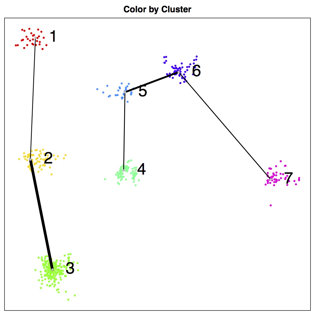
Figure 1: An example for visualizing multivariate mode clustering. This is the Olive Oil data, which has dimension $d=8$. Using the proposed methods in this paper, we identify $7$ clusters and the connections among clusters are represented by edges (width of edge shows the strength of connection). More details can be found in section 8.2.

2 Review of Mode Clustering

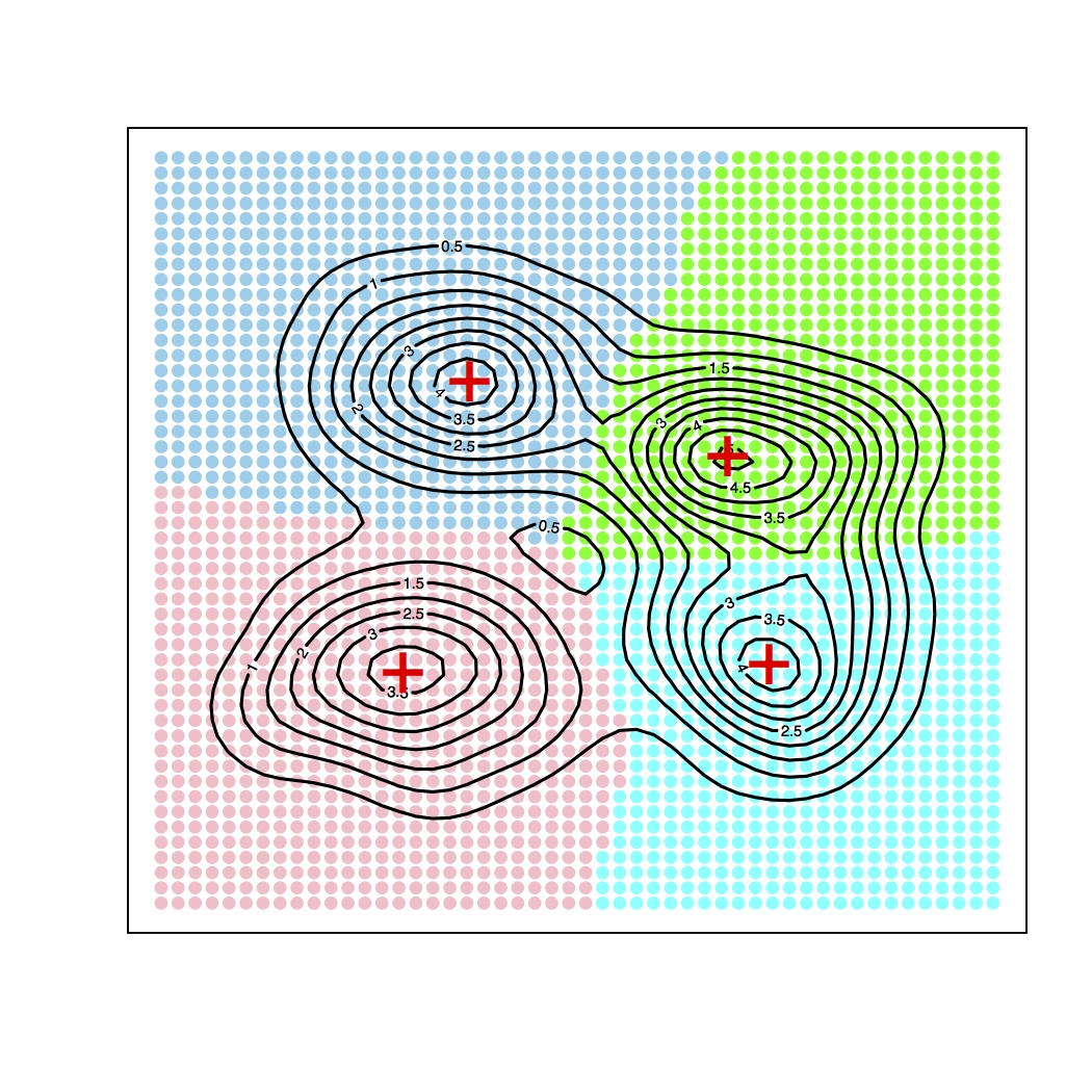
(a) Attraction basins

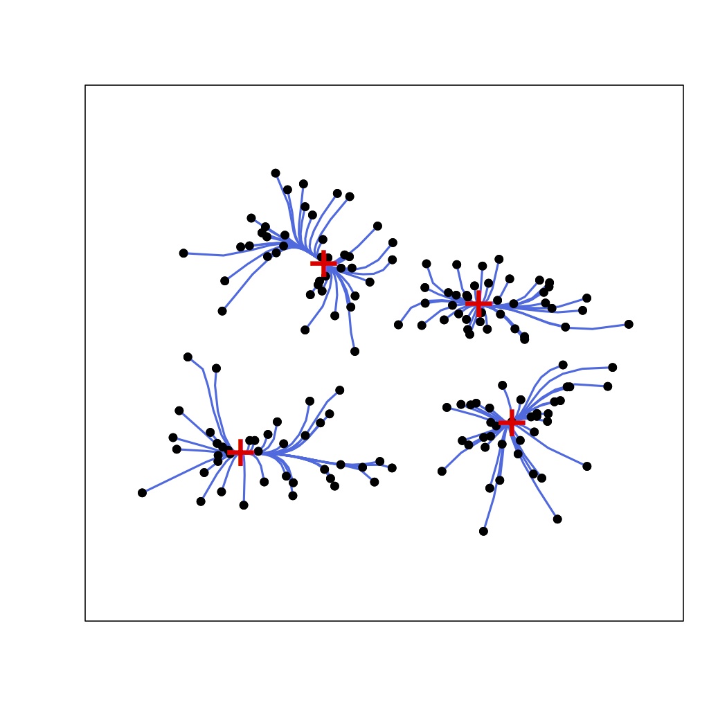
(b) Mean shift

Figure 2: The mode clustering. (a): the attraction basins for each mode given a smooth function. (b): the mean shift algorithm to cluster data points. The red crosses are the local modes.

Let $p$ be the density function of a random vector $X\in\mathbb{R}^{d}$. Throughout the paper, we assume $p$ has compact support $\mathbb{K}\subset\mathbb{R}^{d}$. Assume that $p$ has $k$ local maxima ${\cal M}=\{m_{1},\cdots,m_{k}\}$ and is a Morse function (Morse, 1925, 1930; Banyaga, 2004), meaning that the Hessian of $p$ at each critical point is non-degenerate. We do not assume that $k$ is known. Given any $x\in\mathbb{R}^{d}$, there is a unique gradient ascent path starting at $x$ that eventually arrives at one of the modes (except for a set of $x$’s of measure 0). We define the clusters as the ‘basins of attraction’ of the modes (Chacón, 2012), i.e., the sets of points whose ascent paths have the same mode. Now we give more detail.

An integral curve through $x$ is a path $\pi_{x}:\mathbb{R}\mapsto\mathbb{R}^{d}$ such that $\pi_{x}(0)=x$ and

$$\pi_{x}^{\prime}(t)=\nabla p(\pi_{x}(t)).$$ (1)

A standard result in Morse theory is that integral curves never intersect except at critical points, so the curves partition the space (Morse, 1925, 1930; Banyaga, 2004). We define the destination for the integral curve starting at $x$ by

$$\operatorname{dest}(x)=\underset{t\rightarrow\infty}{\lim}\pi_{x}(t).$$ (2)

Then $\operatorname{dest}(x)=m_{j}$ for some mode $m_{j}$ for all $x$ except on a set $E$ with Lebesgue measure $0$ ($E$ contains points that are on the boundaries of clusters and whose paths lead to saddle points). For each mode $m_{j}$ we define the basin of attraction of $m_{j}$ by

$$C_{j}=\{x:\operatorname{dest}(x)=m_{j}\},\quad j=1,\cdots,k.$$ (3)

$C_{j}$ is also called the ascending manifold (Guest, 2001) or the stable manifold (Morse, 1925, 1930; Banyaga, 2004). The partition ${\cal C}=\{C_{1},\ldots,C_{k}\}$ is called the Morse complex of $p$. These are the population clusters.

In practice, $p(x)$ is unknown and we need to estimate it. A common way to do this is via the kernel density estimator (KDE). Let $X_{1},\ldots,X_{n}$ be a random sample from $p$, and let $K$ be a smooth, symmetric kernel. The KDE with bandwidth $h>0$ is defined by

$$\widehat{p}_{h}(x)=\frac{1}{nh^{d}}\sum_{i}K\left(\frac{||x-X_{i}||}{h}\right).$$ (4)

The modes $\widehat{\cal M}=\{\widehat{m}_{1},\ldots,\widehat{m}_{\widehat{k}}\}$ of $\widehat{p}_{n}$ and the integral-curve destinations under $\widehat{p}_{n}$ of any point $x$, $\widehat{\operatorname{dest}}(x)$, are both easily found using the mean-shift algorithm (Fukunaga and Hostetler, 1975; Cheng, 1995; Comaniciu and Meer, 2002). The corresponding basins of attraction are

$$\widehat{C}_{j} =\{x\in\mathbb{R}^{d}:\;\widehat{\operatorname{dest}}(x)=\widehat{m}_{j}\},\quad j=1,\cdots,{\widehat{k}}$$ (5)

$$\widehat{\cal C} =\{\widehat{C}_{1},\ldots,\widehat{C}_{\widehat{k}}\}$$ (6)

and the sample clusters are defined by

$$\mathcal{X}_{j}=\{X_{i}:\ X_{i}\in\widehat{C}_{j}\}=\{X_{i}:\widehat{\operatorname{dest}}(X_{i})=\widehat{m}_{j}\}.$$ (7)

3 Soft Clustering

Mode clustering is a type of hard clustering, where each observation is assigned to one and only one cluster. Soft clustering methods (McLachlan and Peel, 2004; Lingras and West, 2002; Nock and Nielsen, 2006; Peters et al., 2013) attempt to capture the uncertainty in this assignment. This is typically represented by an assignment vector for each point that is a probability distribution over the clusters. For example, whereas a hard-clustering method might assign a point $x$ to cluster 2, a soft clustering might give $x$ an assignment vector $a(x)=(0.01,0.8,0.01,0.08,0.1)$, reflecting both the high confidence that $x$ belongs to cluster $2$ the nontrivial possibility that it belongs to cluster $5$.

Soft clustering can capture two types of cluster uncertainty: population level (intrinsic difficulty) and sample level (variability). The population level uncertainty originates from the fact that even if $p$ is known, some points are more strongly related to their modes than others. Specifically, for a point $x$ near the boundaries between two clusters, say $C_{1},C_{2}$, the associated soft assignment vector $a(x)$ should have $a_{1}(x)\approx a_{2}(x)$. The sample level uncertainty comes from the fact that $p$ has been estimated by $\widehat{p}$. The soft assignment vector $a(x)$ is designed to capture both types of uncertainty.

Remark: The most common soft-clustering method is to use a mixture model. In this approach, we represent cluster membership by a latent variable and use the estimated distribution of that latent variable as the assignment vector. In the appendix we discuss mixture-based soft clustering.

3.1 Soft Mode Clustering

One way to obtain soft mode clustering is to use a distance from a given point $x$ to all the local modes. The idea is simple: if $x$ is close to a mode $m_{j}$, the soft assignment vector should have a higher $a_{j}(x)$. However, converting a distance to a soft assignment vector involves choosing some tuning parameters.

Instead, we now present a more direct method based on a diffusion that does not require any conversion of distance. Consider starting a diffusion at $x$. We define the soft clustering as the probability that the diffusion starting at $x$ leads to a particular mode, before hitting any other mode. That is, let $a^{HP}(x)=(a^{HP}_{1}(x),\ldots,a^{HP}_{k}(x))$ where $a^{HP}_{j}(x)$ is the conditional probability that mode $j$ is the first mode reached by the diffusion, given that it reaches one of the modes. In this case $a(x)$ is a probability vector and so is easy to interpret.

In more detail, let

$$K_{h}(x,y)=K\left(\frac{\|x-y\|}{h}\right).$$

Then

$$q_{h}(y|x)=\frac{K_{h}(x,y)p(y)}{\int K_{h}(x,y)dP(y)},$$

defines a Markov process with $q_{h}(y|x)$ being the probability of jumping to $y$ given that the process is at $x$. Fortunately, we do not actually have to run the diffusion to estimate $a^{HP}(x)$.

An approximation to the above diffusion process restricted to $x,y$ in $\{\widehat{m}_{1},\ldots,\widehat{m}_{\widehat{k}},X_{1},\ldots,X_{n}\}$ is as follows. We define a Markov chain that has $\widehat{k}+n$ states. The first $\widehat{k}$ states are the estimated local modes $\widehat{m}_{1},\ldots,\widehat{m}_{\widehat{k}}$ and are absorbing states. That is, the Markov process stops when it hits any of the first $\widehat{k}$ state. The other $n$ states correspond to the data points $X_{1},\ldots,X_{n}$. The transition probability from each $X_{i}$ is given by

$$\mathbf{P}(X_{i}\rightarrow\widehat{m}_{l}) =\frac{K_{h}(X_{i},\widehat{m}_{j})}{\sum_{j=1}^{n}K_{h}(X_{i},X_{j})+\sum_{l=1}^{\widehat{k}}K_{h}(X_{i},\widehat{m}_{l})}$$ (8)

$$\mathbf{P}(X_{i}\rightarrow X_{j}) =\frac{K_{h}(X_{i},X_{j})}{\sum_{j=1}^{n}K_{h}(X_{i},X_{j})+\sum_{l=1}^{\widehat{k}}K_{h}(X_{i},\widehat{m}_{l})}$$

for $i,j=1,\ldots,n$ and $l=1,\ldots,\widehat{k}$. Thus, the transition matrix $\mathbf{P}$ is

$$\mathbf{P}=\begin{bmatrix}\mathbf{I}&0\\ S&T\end{bmatrix},$$ (9)

where $\mathbf{I}$ is the identity matrix and $S$ is an $n\times\widehat{k}$ matrix with element $S_{ij}=\mathbf{P}(X_{i}\rightarrow\widehat{m}_{j})$ and $T$ is an $n\times n$ matrix with element $T_{ij}=\mathbf{P}(X_{i}\rightarrow X_{j})$. Then by Markov chain theory, the absorbing probability from $X_{i}$ onto $\widehat{m}_{j}$ is given by $\widehat{A}_{ij}$ where $\widehat{A}_{ij}$ is the $(i,j)$-th element of the matrix

$$\widehat{A}=S(\mathbf{I}-T)^{-1}.$$ (10)

We define the soft assignment vector by $\widehat{a}^{HP}_{j}(X_{i})=\widehat{A}_{ij}$.

4 Measuring Cluster Connectivity

In this section, we propose a technique that uses the soft-assignment vector to measure the connectivity among clusters. Note that the clusters here are generated by the usual (hard) mode clustering.

Let $p$ be the density function and $C_{1},\ldots,C_{k}$ be the clusters corresponding to the local modes $m_{1},\ldots,m_{k}$. For a given soft assignment vector $a(x):\mathbb{R}^{d}\mapsto\mathbb{R}^{k}$, we define the connectivity of cluster $i$ and cluster $j$ by

$$\Omega_{ij} =\frac{1}{2}\Bigl{(}\mathbb{E}\bigl{(}a_{i}(X)|X\in C_{j}\bigr{)}+\mathbb{E}\bigl{(}a_{j}(X)|X\in C_{i}\bigr{)}\Bigr{)}$$ (11)

$$=\frac{1}{2}\frac{\int_{C_{i}}a_{j}(x)p(x)dx}{\int_{C_{i}}p(x)dx}+\frac{1}{2}\frac{\int_{C_{j}}a_{i}(x)p(x)dx}{\int_{C_{j}}p(x)dx}.$$

Each $\Omega_{ij}$ is a population level quantity that depends only on how we determine the soft assignment vector. Connectivity will be large when two clusters are close and the boundary between them has high density. If we think of the (hard) cluster assignments as class labels, connectivity is analogous to the mis-classification rate between class $i$ and class $j$.

An estimator of $\Omega_{ij}$ is

$$\widehat{\Omega}_{ij}=\frac{1}{2}\Bigl{(}\frac{1}{N_{i}}\sum_{l=1}^{n}\widehat{a}_{j}(X_{l})1(X_{l}\in\widehat{C}_{i})+\frac{1}{N_{j}}\sum_{l=1}^{n}\widehat{a}_{i}(X_{l})1(X_{l}\in\widehat{C}_{j})\Bigr{)},\quad i,j=1,\ldots,\widehat{k},$$ (12)

where $N_{i}=\sum_{l=1}^{n}1(X_{l}\in\widehat{C}_{i})$ is the number of sample in cluster $\widehat{C}_{i}$. Note that when $n$ is sufficiently large, each estimated mode is a consistent estimator to one population mode (Chazal et al., 2014) but the ordering might be different. For instance, the first estimated mode $\widehat{m}_{1}$ might be the estimator for the third population mode $m_{3}$. After relabeling, we can match the ordering of both population and estimated modes. Thus, after permutation of columns and rows of $\widehat{\Omega}$, $\widehat{\Omega}$ will be a consistent estimator to $\Omega$. The matrix $\widehat{\Omega}$ is a summary statistics for the connectivity between clusters. We call $\widehat{\Omega}$ the matrix of connectivity or the connectivity matrix.

The matrix $\widehat{\Omega}$ is useful as a dimension-free, summary-statistic to describe the degree of overlap/interaction among the clusters, which is hard to observe directly when $d>2$. Later we will use $\widehat{\Omega}$ to describe the relations among clusters while visualizing the data.

5 Consistency

Local modes play a key role in mode clustering. Here we discuss the consistency of mode estimation. Despite the fact that the consistency for estimating a global mode has been established (Romano, 1988; Romano et al., 1988; Pollard, 1985; Arias-Castro et al., 2013; Chacon, 2014; Chazal et al., 2014; Chen et al., 2014a), there is less work on estimating local modes .

Here we adapt the result in Chen et al. (2014c) to describe the consistency of estimating local modes in terms of the Hausdorff distance. For two sets $A,B$, the Hausdorff distance is

$${\sf Haus}(A,B)=\inf\{r:A\subset B\oplus r,B\subset A\oplus r\},$$ (13)

where $A\oplus r=\{y:\min_{x\in A}\|x-y\|\leq r\}$. The Hausdorff distance is a generalized $L_{\infty}$ metric for sets.

Let $K^{(\alpha)}$ be the $\alpha$-th derivative of $K$ and $\mathbf{BC}^{r}$ denotes the collection of functions with bounded continuously derivatives up to the $r$-th order. We consider the following two common assumptions on kernel function:

• The kernel function $K\in\mathbf{BC}^{3}$ and is symmetric, non-negative and

  $$\int x^{2}K^{(\alpha)}(x)dx<\infty,\qquad\int\left(K^{(\alpha)}(x)\right)^{2}dx<\infty$$

  for all $\alpha=0,1,2,3$.

• The kernel function satisfies condition $K_{1}$ of Gine and Guillou (2002). That is, there exists some $A,v>0$ such that for all $0<\epsilon<1$, $\sup_{Q}N(\mathcal{K},L_{2}(Q),C_{K}\epsilon)\leq\left(\frac{A}{\epsilon}\right)^{v},$ where $N(T,d,\epsilon)$ is the $\epsilon-$covering number for a semi-metric space $(T,d)$ and

  $$\mathcal{K}=\Biggl{\{}u\mapsto K^{(\alpha)}\left(\frac{x-u}{h}\right):x\in\mathbb{R}^{d},h>0,|\alpha|=0,1,2,3\Biggr{\}}.$$

The assumption (K1) is a smoothness condition on the kernel function. (K2) controls the complexity of the kernel function and is used in (Gine and Guillou, 2002; Einmahl and Mason, 2005; Genovese et al., 2012; Arias-Castro et al., 2013; Chen et al., 2014b).

Theorem 1 (Consistency of Estimating Local Modes).

Assume $p\in\mathbf{BC}^{3}$ and the kernel function $K$ satisfies (K1-2). Let $C_{3}$ be the bound for the partial derivatives of $p$ up to the third order and $\widehat{\mathcal{M}}_{n}\equiv\widehat{\mathcal{M}}$ be the collection of local modes of the KDE $\widehat{p}_{n}$ and $\mathcal{M}$ be the local modes of $p$. Let $\widehat{K}_{n}$ be the number of estimated local modes and $K$ be the number of true local modes. Assume

• There exists $\lambda_{*}>0$ such that

  $$0<\lambda_{*}\leq|\lambda_{1}(m_{j})|,\quad j=1,\cdots,k,$$

  where $\lambda_{1}(x)\leq\cdots\leq\lambda_{d}(x)$ are the eigenvalues of Hessian matrix of $p(x)$.

• There exists $\eta_{1}>0$ such that

  $$\{x:\|\nabla p(x)\|\leq\eta_{1},0>-\lambda_{*}/2\geq\lambda_{1}(x)\}\subset\mathcal{M}\oplus\frac{\lambda_{*}}{2dC_{3}},$$

  where $\lambda_{*}$ is defined in (M1).

Then when $h$ is sufficiently small and $n$ is sufficiently large,

• (Modal consistency) there exists some constants $A,C>0$ such that

  $$\mathbb{P}\left(\widehat{k}_{n}\neq k\right)\leq Ae^{-Cnh^{d+4}};$$

• (Location convergence) the Hausdorff distance between local modes and their estimators satisfies

  $${\sf Haus}\left(\widehat{\mathcal{M}}_{n},\mathcal{M}\right)=O(h^{2})+O_{P}\left(\sqrt{\frac{1}{nh^{d+2}}}\right).$$

The proof is in appendix. Actually, the assumption (M1) always hold whenever we assume $p$ to be a Morse function. We make it an assumption just for the convenience of the proof. The second condition (M2) is a regularity on $p$ which requires that points with similar behavior (near $0$ gradient and negative eigenvalues) to local modes must be close to local modes. Theorem 1 states two results: consistency for estimating the number of local modes and consistency for estimating the location of local modes. An intuitive explanation for the first result is from the fact that as long as the gradient and Hessian matrix of KDE $\widehat{p}_{n}$ are sufficiently closed to the true gradient and Hessian matrix, condition (M1, M2) guarantee the number of local modes is the same as truth. Applying Talagrand’s inequality (Talagrand, 1996) we obtain exponential concentration which gives the desired result. The second result follows from applying a Taylor expansion of the gradient around each local mode, the difference between local modes and their estimators is proportional to the error in estimating the gradients. The Hausdorff distance can be decomposed into bias $O(h^{2})$ and variance $O_{P}\left(\sqrt{\frac{1}{nh^{d+2}}}\right)$.

5.1 Bandwidth Selection

A key problem in mode clustering is the choice of the smoothing bandwidth $h$. Because mode clustering is based on the gradient of the density function, we choose a bandwidth targeted at gradient estimation. From standard non-parametric density estimation theory, the estimated gradient and the true gradient differ by

$$\|\nabla\widehat{p}_{n}(x)-\nabla p(x)\|^{2}_{2}=O(h^{4})+O_{P}\Bigl{(}\frac{1}{nh^{d+2}}\Bigr{)}$$ (14)

assuming $p$ has two smooth derivatives, see Chacón et al. (2011); Arias-Castro et al. (2013). In non-parametric literature, a common error measure is the mean integrated square error (MISE). The MISE for the gradient is

$${\sf MISE}(\nabla\widehat{p}_{n})=\mathbb{E}\left(\int\|\nabla\widehat{p}_{n}(x)-\nabla p(x)\|^{2}_{2}dx\right)=O\left(h^{4}\right)+O\left(\frac{1}{nh^{d+2}}\right)$$ (15)

when we assume (K1); see Theorem 4 of (Chacón et al., 2011). Thus, it follows that the asymptotically optimal bandwidth should be

$$h=Cn^{-\frac{1}{d+6}},$$ (16)

for some constant $C$. In practice, we do not know $C$, so we need a concrete rule to select it. We recommend a normal reference rule (a slight modification of Chacón et al. (2011)):

$$h_{NR}=\bar{S}_{n}\times\Bigl{(}\frac{4}{d+4}\Bigr{)}^{\frac{1}{d+6}}n^{-\frac{1}{d+6}},\qquad\bar{S}_{n}=\frac{1}{d}\sum_{j=1}^{d}S_{n,j}$$ (17)

where $S_{n,j}$ is the sample standard deviation along $j$-th coordinate. We use this for two reasons. First, it is known that the normal reference rule tends to oversmooth (Sheather, 2004), which is typically good for clustering. And second, the normal reference rule is easy to compute even in high dimensions. Note that this normal reference rule is optimizing asymptotic MISE for multivariate Gaussian distirbution with covariance matrix $\sigma\mathbf{I}$. Corollary 4 of Chacón et al. (2011) provides a formula for the general covariance matrix case. In data analysis, it is very common to normalize the data first and then perform mode clustering. If we normalize the data, the reference rule (17) reduces to $h_{NR}=\Bigl{(}\frac{4}{d+4}\Bigr{)}^{\frac{1}{d+6}}n^{-\frac{1}{d+6}}$. For a comprehensive survey on the bandwidth selection, we refer the readers to Chacón and Duong (2013).

In addition to the MISE, another common metric for measuring the quality of the estimator $\nabla\widehat{p}_{n}$ is the ${\cal L}^{\infty}$ norm, which is defined by

$$\|\nabla\widehat{p}_{n}-\nabla p\|_{\max,\infty}=\sup_{x}\|\nabla\widehat{p}_{n}(x)-\nabla p(x)\|_{\max},$$ (18)

where $\|v\|_{\max}$ is the maximal norm for a vector $v$.

The rate for ${\cal L}^{\infty}$ is

$$\|\nabla\widehat{p}_{n}-\nabla p\|_{\max,\infty}=O\left(h^{2}\right)+O_{P}\left(\sqrt{\frac{\log n}{nh^{d+2}}}\right)$$ (19)

when we assume (K1–2) and $p\in\mathbf{BC}^{3}$ (Genovese et al., 2009, 2012; Arias-Castro et al., 2013; Chen et al., 2014b). This suggests selecting the bandwidth by

$$h=C^{\prime}\left(\frac{\log n}{n}\right)^{\frac{1}{d+6}}.$$ (20)

However, no general rule has been proposed based on this norm. The main difficulty is that no analytical form for the big $O$ term has been found.

Remark. Comparing the assumptions in Theorem 1, equations (15) and 19 gives an interesting result: If we assume $p\in\mathbf{BC}^{3}$ and (K1), we obtain consistency in terms of the MISE. If further we assume (K2), we get the consistency in terms of the supremum-norm. Finally, if we have conditions (M1-2), we obtain mode consistency.

6 Denoising Small Clusters

In high dimensions, mode clustering tends to produce many small clusters , that is, clusters with few data points. We call these small clusters, clustering noise. In high dimensions, the variance creates small bumps in the KDE which then creates clustering noise. The emergence of clustering noise is consistent with Theorem 1; the convergence rate is much slower when $d$ is high.

Figure 3 gives an example on the small clusters from a 4-Gaussian mixture and each mixture component contains $200$ points. Note that this mixture is in $d=8$ and the first two coordinates are given in panel (a) of Figure 3. Panel (b) shows the ordered size of clusters when the smoothing parameter $h$ is chosen by the Silverman’s rule (SR) given in (17). On the left side of the gray vertical line, the four clusters are real signals while the clusters on the right hand side of the gray line are small clusters that we want to filter out.

(a) Scatter plot for first two coordinates

(b) Ordered size of clusters

Figure 3: An example of cluster noise. These data are from a 4-Gaussian mixture in $d=8$. Panel (a) shows the first two coordinates and we add Gaussian noise to other $6$ coordinates. Panel (b) shows the ordered size of clusters from mode clustering using Silverman’s rule (17). On the left side of gray line in panel (b) are the real clusters; on the right side of gray line are the clusters we want to filter out.

There are two approaches to deal with the clustering noise: increasing the smoothing parameters and merging (or eliminating) small clusters. However, increasing the bandwidth oversmooths which may wash out useful information. See Figure 4 for an example. Thus, we focus on the method of merging small clusters. Our goal is to have a quick, simple method.

Figure 4: An example for showing the problem of oversmoothing. This is a $n=100$ sample from a simple two Gaussian mixture in $d=1$. The black curve is the true density, the blue curve is the estimated density based on the Silverman’s rule (denoted as SR; see (17)) and the orange curve is $h=1.3\times$ (17). If we oversmooth too much (orange curve), we only identify one cluster (mode).

A simple merging method is to enforce a threshold $n_{0}$ on the cluster size (i.e., number of data points within) and merge points within the small clusters (size less than $n_{0}$) into some nearby clusters whose size is larger or equal to $n_{0}$. We will discuss how to merge tiny clusters latter. Clusters with size larger or equal to $n_{0}$ are called “significant” clusters and those with size less than $n_{0}$ are called “insignificant” clusters. We recommend setting

$$n_{0}=\left(\frac{n\log(n)}{20}\right)^{\frac{d}{d+6}}.$$ (21)

The intuition for the above rule is from the optimal $L_{\infty}$ error rate for estimating the gradient (recall (19)). The constant $20$ in the denominator is based on our experience from simulations and later, we will see that this rule works quiet well in practice.

Here we introduce the SC-plot (Size of Cluster plot) as a diagnostic for the choice of $n_{0}$. The SC-plot displays the ordered size of clusters. Ideally, there will be a gap between the size of significant clusters and insignificant clusters which in turns induces an elbow in the SC-plot. Figure 5 show the SC-plot for a 4-Gaussian mixture in 8-dimension (the data used in Figure 3) and a 5-clusters in 10-dimension data (see section 8.1 for more details). Both data sets are simulated so that we know the true number of clusters (we use the gray line to separate clustering noise and real clusters). Our reference rule (21) successfully separates the noise and signals in both cases. Note that SC-plot itself provides a summary of the structure of clusters.

After identifying tiny clusters, we use the following procedure to merge points within small clusters (suggested to us by Jose Chacon). We first remove points in tiny clusters and then use the remaining data (we call this the “reduced dataset”) to estimate the density and perform mode clustering. Since the reduced dataset does not include points within tiny clusters, in most cases, this method outputs only stable clusters. If there are still tiny clusters after merging, we identify those points within tiny clusters and merge them again to other large clusters. We repeat this process until there are no tiny clusters. By doing so, we will cluster all data points into significant clusters.

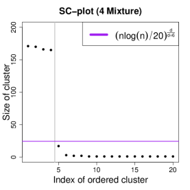
(a) SC-plot for 4-Gaussian in 8-D

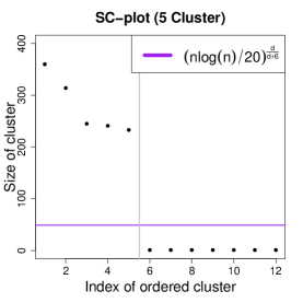
(b) SC-plot for 5-clusters in 10-D

Figure 5: The SC-plot for the 4-Gaussian example and the 5-clusters in 10-D example. Notice that there is always a gap on the size of clusters near the gray line (boundary of real clusters and clustering noise). This gap can be used to select the filtering threshold $n_{0}$.

Remark. In addition to the denoising method proposed above, we can remove the clustering noise using persistent homology (Chazal et al., 2011). The threshold level for persistence can be computed via the bootstrap (Fasy et al., 2014). However, we found that this did not work well except in low dimensions. Also, it is extremely computationally intensive.

7 Visualization

Here we present a method for visualizing the clusters that combines multidimensional scaling (MDS) with our connectivity measure for clusters.

7.1 Review of Multidimensional Scaling

Given points $X_{1},\ldots,X_{n}\in\mathbb{R}^{d}$, classical MDS finds $Z_{1},\ldots,Z_{n}\in\mathbb{R}^{k}$ such that they minimize

$$\sum_{i,j}\left|(Z_{i}-\bar{Z}_{n})^{T}(Z_{j}-\bar{Z}_{n})-(X_{i}-\bar{X}_{n})^{T}(X_{j}-\bar{X}_{n})\right|^{2}.$$ (22)

Note $\bar{Z}_{n}=\frac{1}{n}\sum_{i=1}^{n}Z_{i}$. A nice feature for classical MDS is the existence of a closed-form solution to $Z_{i}$’s. Let $\mathbf{S}$ be a $n\times n$ matrix with element

$$\mathbf{S}_{ij}=(X_{i}-\bar{X}_{n})^{T}(X_{j}-\bar{X}_{n}).$$

Let $\lambda_{1}>\lambda_{2}>\cdots>\lambda_{n}$ be the eigenvalues of $\mathbf{S}$ and $v_{1},\ldots,v_{n}\in\mathbb{R}^{n}$ be the associated eigenvectors. We denote $\mathbf{V}_{k}=[v_{1},\ldots,v_{k}]$ and $\mathbf{D}_{k}={\sf Diag}(\sqrt{\lambda_{1}},\ldots,\sqrt{\lambda_{k}})$ be a $k\times k$ diagonal matrix. Then it is known that each $Z_{i}$ is the $i$-th row of $\mathbf{V}_{k}\mathbf{D}_{k}$ (Hastie et al., 2001). In our visualization, we constrain $k=2$.

7.2 Two-stage Multidimensional Scaling

Our approach consists of two stages. At the first stage, we apply MDS on the modes and plot the result in $\mathbb{R}^{2}$. At the second stage, we apply MDS to points within each cluster along with the associated mode. Then we place the points around the projected modes. We scale the MDS result at the first stage by a factor $\rho_{0}$ so that each cluster is separated from each other. Figure 6 gives an example.

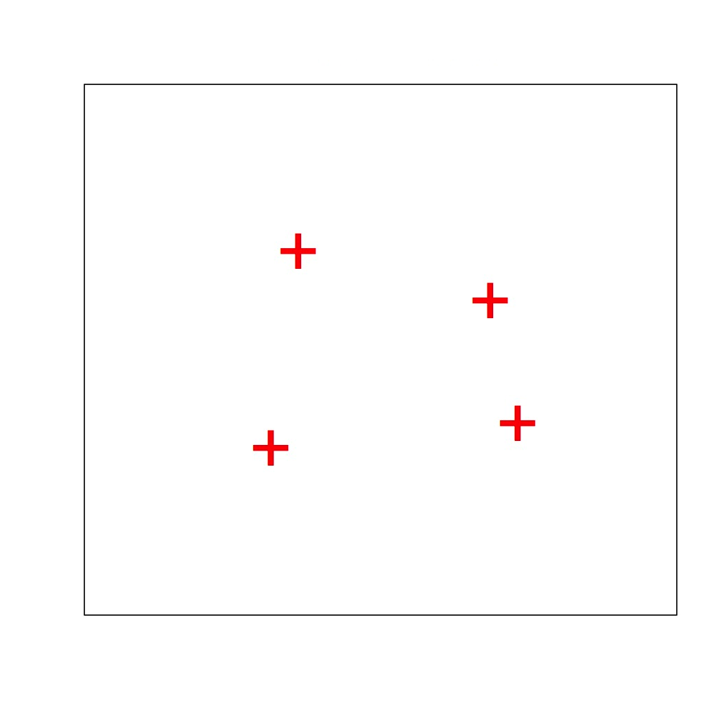
(a) MDS on modes

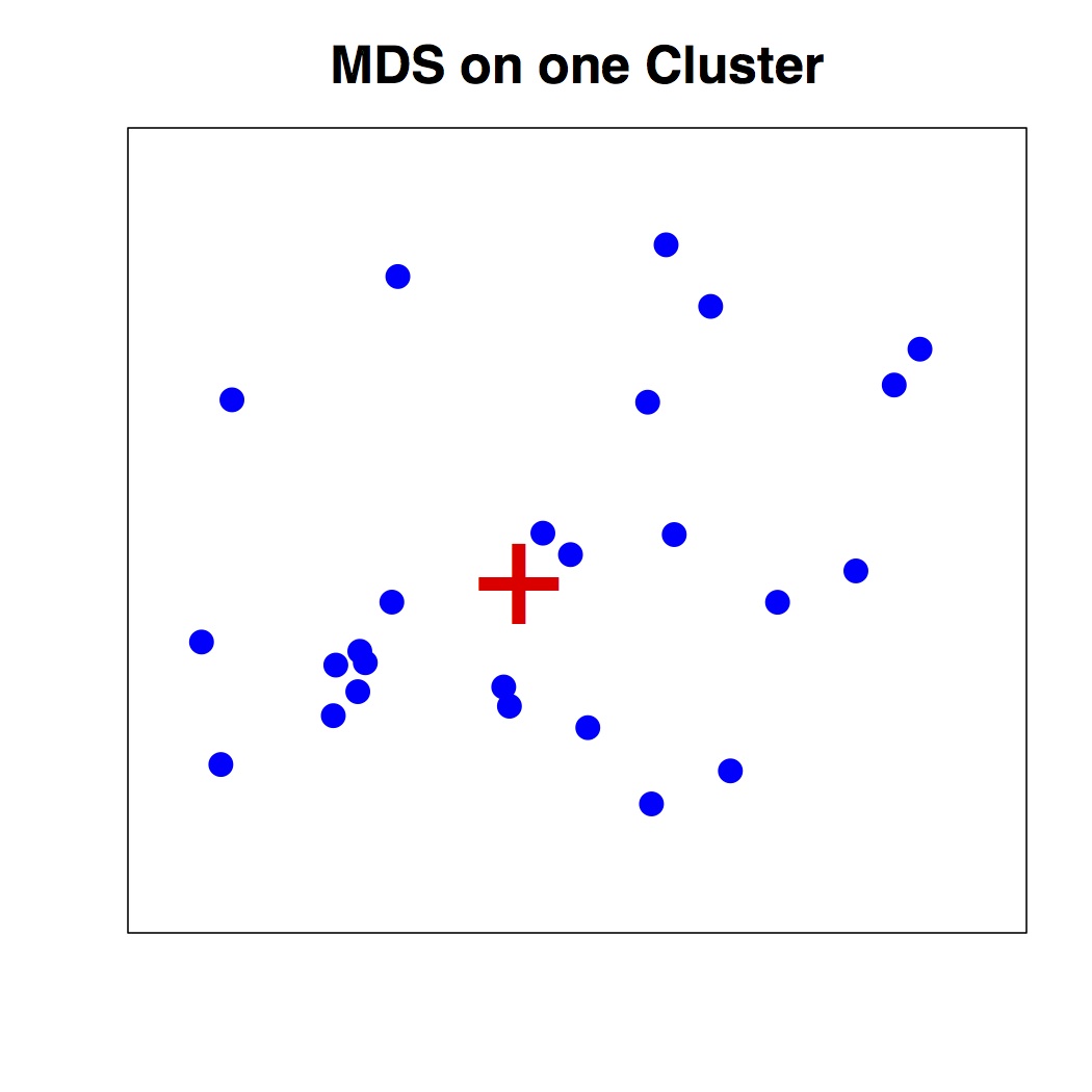
(b) MDS on each cluster

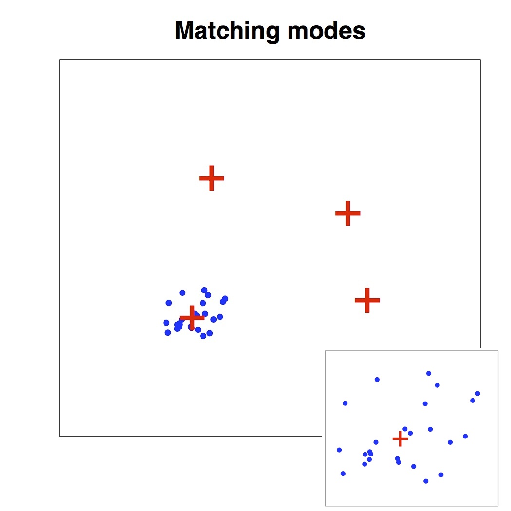
(c) Place points around modes

(d) The final result

Figure 6: An example for the two stage MDS. Note that the bottom right small plot in (c) is the plot in (b). At stage one, we run MDS for all modes and plot them as in (a). At stage two, we apply MDS for each cluster including the local mode as in (b). Then we place cluster points around local modes as in (c) and (d).

Recall that $\widehat{\cal M}=\{\widehat{m}_{1},\ldots,\widehat{m}_{\widehat{k}}\}$ is the set of estimated local modes and $\mathcal{X}_{j}$ is the set of data points belonging to mode $\widehat{m}_{j}$. At the first stage, we perform MDS on $\widehat{\cal M}$ so that

$$\{\widehat{m}_{1},\ldots,\widehat{m}_{\widehat{k}}\}\overset{{\sf MDS}}{\Longrightarrow}\{\widehat{m}^{\dagger}_{1},\ldots,\widehat{m}^{\dagger}_{\widehat{k}}\},$$ (23)

where $\widehat{m}^{\dagger}_{j}\in\mathbb{R}^{2}$ for $j=1,\ldots,\widehat{k}.$ We plot $\{\widehat{m}^{\dagger}_{1},\ldots,\widehat{m}^{\dagger}_{\widehat{k}}\}$.

At the second stage, we consider each cluster individually. Assume we are working on the $j$-th cluster and $\widehat{m}_{j},\mathcal{X}_{j}$ are the corresponding local mode and cluster points. We denote $\mathcal{X}_{j}=\{X_{j1},\ldots,X_{jN_{j}}\}$, where $N_{j}$ is the sample size for cluster $j$. Then we apply MDS to the collection of points $\{m_{j},X_{j1},X_{j2},\ldots,X_{jN_{j}}\}$:

$$\{m_{j},X_{j1},X_{j2},\ldots,X_{jN_{j}}\}\overset{{\sf MDS}}{\Longrightarrow}\{m^{*}_{j},X^{*}_{j1},X^{*}_{j2},\ldots,X^{*}_{jN_{j}}\},$$ (24)

where $m^{*}_{j},X^{*}_{j1},X^{*}_{j2},\ldots,X^{*}_{jN_{j}}\in\mathbb{R}^{2}$. Then we center the points at $\widehat{m}^{\dagger}_{j}$ and place $X^{*}_{j1},X^{*}_{j2},\ldots,X^{*}_{jN_{j}}$ around $\widehat{m}^{\dagger}_{j}$. That is, we make a translation to the set $\{m^{*}_{j},X^{*}_{j1},X^{*}_{j2},\ldots,X^{*}_{jN_{j}}\}$ so that $m^{*}_{j}$ matches the location of $\widehat{m}^{\dagger}_{j}$. Then we plot the translated points $X^{*}_{j1},X^{*}_{j2},\ldots,X^{*}_{jN_{j}}$. We repeat the above process for each cluster to visualize the high dimensional clustering.

Note that in practice, the above process may cause unwanted overlap among clusters. Thus, one can scale $\{\widehat{m}^{\dagger}_{1},\ldots,\widehat{m}^{\dagger}_{\widehat{k}}\}$ by a factor $\rho_{0}>1$ to remove the overlap.

One can use other dimension reduction techniques as well. For instance, we can use the landmark MDS (Silva and Tenenbaum, 2002; De Silva and Tenenbaum, 2004) and treats each local mode as the landmark points. This provides an alternative way to visualize the clusters.

7.3 Connectivity Graph

We can improve the visualization of the previous subsection by accounting for the connectivity of the clusters. We apply the connectivity measure introduced in section 4. Let $\widehat{\Omega}$ be the matrix for the connectivity measure defined in (12). We connect two clusters, say $i$ and $j$, by a straight line if the connectivity measure $\widehat{\Omega}_{ij}>\omega_{0}$, a pre-specified threshold. Our experiments show that

$$\omega_{0}=\frac{1}{2\times\mbox{number of clusters}}$$ (25)

is a good default choice. We can adjust the width of the connection line between clusters to show the strength of connectivity. See Figure 10 panel (a) for an example; the edge linking clusters (2,3) is much thicker than any other edge.

Algorithm 1 summarizes the process of visualizing high dimensional clustering. Note that the smoothing bandwidth $h$ and the thresholding of cluster size $n_{0}$ can be chosen by the methods proposed in section 5.1. The remaining two parameters $\rho_{0}$ and $\omega_{0}$ are visualization parameters; they are not involved in any analysis so that one can change these parameters freely.

Algorithm 1 Visualization for Mode Clustering

Input: Data $\mathbb{X}=\{X_{i}:i=1,\ldots,n\}$, bandwidth $h$, parameters $n_{0}$, $\rho_{0}$, $\omega_{0}$.

Phase 1: Mode clustering

1. Use the mean shift algorithm for clustering based on bandwidth $h$.

2. (Optional) Find clusters of size less than $n_{0}$ and merge them with larger clusters.

Phase 2: Dimension reduction

Let $\{(m_{j},\mathcal{X}_{j}):j=1,\ldots,\widehat{k}\}$ be the pairs of local modes and the associated data points.

3. Perform MDS to each $(\widehat{m}_{j},\mathcal{X}_{j})$ to get $(\widehat{m}^{*}_{j},\mathcal{X}^{*}_{j})$.

4. Perform MDS to modes only to get $\{\widehat{m}^{\dagger}_{1},\ldots,\widehat{m}^{\dagger}_{\widehat{k}}\}$.

5. Place each $\widehat{M}^{\dagger}_{j}=\rho_{0}\times\widehat{m}^{\dagger}_{j}$ on the reduced coordinate.

6. Place each $(\widehat{m}_{j},\mathcal{X}_{j})$ around $\widehat{M}^{\dagger}_{j}$ by matching $\widehat{m}_{j}\rightarrow\widehat{M}^{\dagger}_{j}$.

Phase 3: Connectivity measure

7. Estimate $\Omega_{ij}$ by (12) and one of the above soft clustering methods.

8. Connect $\widehat{M}^{\dagger}_{i},\widehat{M}^{\dagger}_{j}$ if $\widehat{\Omega}_{ij}>\omega_{0}$.

8 Experiments

We present several experiments in this section. The parameters were chosen as follows: we choose $h$ based on (17), $\omega_{0}$ based on (25). Figure 7 gives a flowchart that summarizes clustering analysis using the approach presented in this paper. Given the multivariate data, we first select the bandwidth and then conduct (hard) mode clustering. Having identified clusters, we denoise small clusters by merging them into significant clusters and apply soft-mode clustering to measure the connectivity. Finally, we visualize the data using the two-step MDS approach and connect clusters if the pairwise connectivity is high. This establishes a procedure for multivariate clustering and we apply it to the data in Sections 8.1 to 8.5.

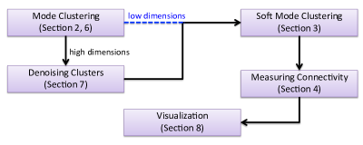
Figure 7: A flowchart for the clustering analysis using proposed methods. This shows a procedure to conduct a high-dimensional clustering using the proposed methods in the current papers. We apply this procedure to the data in section 8.1 to 8.5.

8.1 5-clusters in 10-D

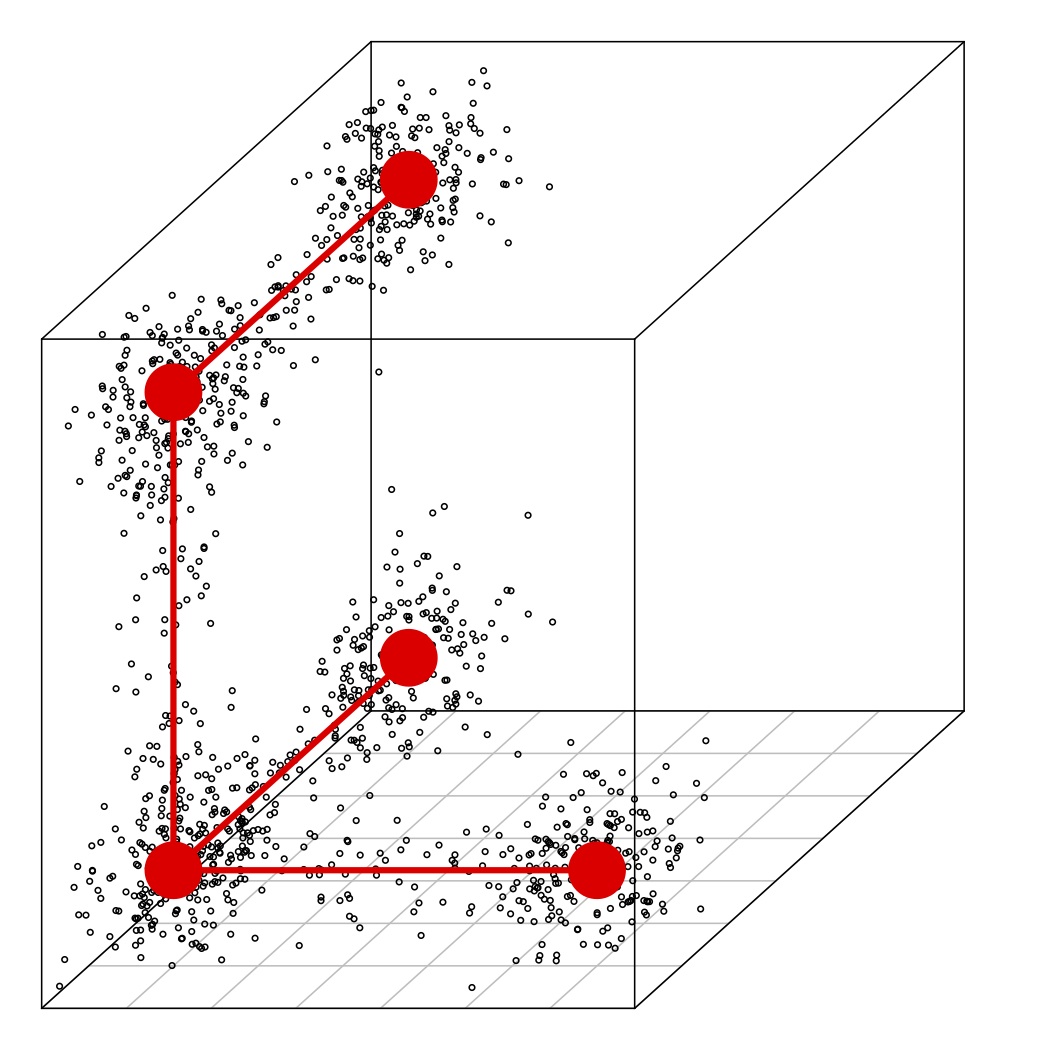
(a) The first three coordinates.

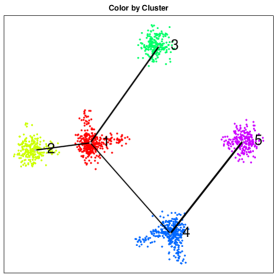
(b) Visualization

	1	2	3	4	5
1	–	0.15	0.14	0.12	0.02
2	0.15	–	0.03	0.03	0.00
3	0.14	0.03	–	0.02	0.00
4	0.12	0.03	0.02	–	0.16
5	0.02	0.00	0.00	0.16	–

(c) Matrix of connectivity

Figure 8: Visualization of clustering on the 10-dimensional 5-cluster data. This is a 5 cluster data with ‘filament’ connecting them in $d=10$. Panel (a) shows the first three coordinates (which contains real structures; the rest $7$ dimensions are Gaussian noise).

We implement our visualization technique in the following ‘5-cluster’ data. We consider $d=10$ and $5$ Gaussian mixture centered at the following positions

$$C_{1} =(0,0,0,0,0,0,0,0,0,0)$$ (26)

$$C_{2} =(0.1,0,0,0,0,0,0,0,0,0)$$

$$C_{3} =(0,0.1,0,0,0,0,0,0,0,0)$$

$$C_{4} =(0,0,0,0.1,0,0,0,0,0,0)$$

$$C_{5} =(0,0.1,0.1,0,0,0,0,0,0,0).$$

For each Gaussian component, we generate $200$ data points from $\sigma_{1}=0.01$ and each Gaussian is isotropically distributed. Then we consider four “edges” connecting pairs of centers. These edges are $E_{12},E_{13},E_{14},E_{45}$, where $E_{ij}$ is the edge between $C_{i},C_{j}$. We generate $100$ points from an uniform distribution over each edge and add an isotropic iid Gaussian noise to each edge with $\sigma_{2}=0.005$. Thus, the total sample size is $1,400$ and consist of 5 clusters centered at each $C_{i}$ and part of the clusters are connected by a ‘noisy path’ (also called filament (Genovese et al., 2012; Chen et al., 2014b)). The density has structure only at the first three coordinates; a visualization for the structure is given in Figure 8-(a).

The goal is to identify the five clusters as well as their connectivity. We display the visualization and the connectivity measures in Figure 8. All the parameters used in this analysis is given as follows.

$$h=0.0114,\quad n_{0}=49.05,\quad\quad\rho_{0}=2,\quad\omega_{0}=0.1.$$

Note that the filtering threshold $n_{0}$ is picked by (21) and the SC-plot is given in Figure 5 panel (b).

8.2 Olive Oil Data

We apply our methods to the Olive Oil data introduced in Forina et al. (1983). This data set consists of 8 chemical measurements (features) for each observation and the total sample size is $n=572$. Each observation is an olive oil produced in one of 3 regions in Italy and these regions are further divided into 9 areas. Some other analyses for this data can be found in Stuetzle (2003); Azzalini and Torelli (2007). We hold out the information of the areas and regions and use only the 8 chemical measurement to cluster all the data.

Since these measurements are in different units, we normalize and standardize each measurement. We apply (17) for selecting $h$ and thresholding the size of clusters based on (21). Figure 9 shows the SC-plot and the gap occurs between the seventh (size: $29$) and eighth cluster (size: $6$) and our threshold $n_{0}=19.54$ is within this gap. We move the insignificant clusters into the nearest significant clusters. After filtering, 7 clusters remain and we apply algorithm 1 for visualizing these clusters. To measure the connectivity, we apply the hitting probability so that we do not have to choose the constant $\beta_{0}$. To conclude, we use the following parameters

$$h=0.587,\quad n_{0}=19.54,\quad\rho_{0}=6,\quad\omega_{0}=0.071.$$

The visualization is given in Figure 10 and matrix of connectivity is given in Figure 11. We color each point according to the produced area to see how our methods capture the structure of data.

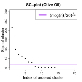
Figure 9: The SC-plot for Olive Oil data. The threshold $n_{0}=19.54$ is within the a gap ($29$ to $6$) between size of seventh and eighth cluster.

As can be seen, most clusters contain one dominating type of olive oil (type: produce area). Even in cases where one cluster contains multiple types of olive oil, the connectivity matrix captures this phenomena. For instance, cluster 2 and 3 both contain Calabria, Sicily and South-Apulia. We do observe a connection between cluster 2 and 3 in Figure 11 and a higher connectivity measure in the matrix for connectivity measures. We display the map of Italy in panel (b) of Figure 10. Mode clustering and connectivity measures reflect the relationship in terms of geographic distance.

As can be seen in Figure 10, the clustering indeed captures the difference in produce area. More importantly, the connectivity measurement captures the hidden structures of the produce area in the following sense. When a group of oil produced in the same area is separated into two clusters, we observe an edge between these two clusters. This shows that the connectivity measure conveys more information on the hidden interaction between clusters.

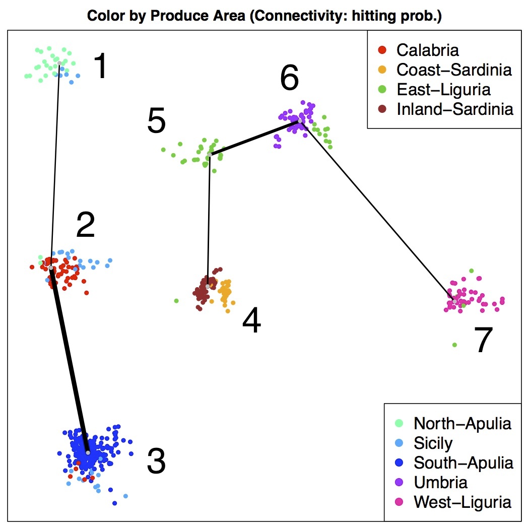
(a) Visualization

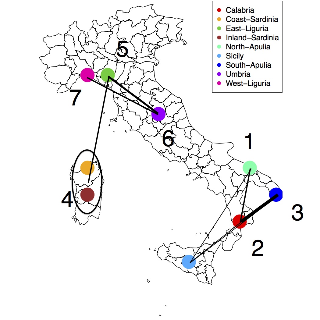
(b) Map of produce area

Figure 10: (a): Clustering result for the Olive oil data ($d=8$). Note that we add edges to those pairs of clusters with connectivity measure $>0.07$ (colored by red in the matrix). The connectivity matrix is in Figure 11. The width of the edge reflects the degree of connection. (b): The corresponding map of Italy. We assign the cluster label to the dominating produce area and connect the edge according to the connectivity matrix. Note that the Sicily is spread out over cluster 1-3 so that we use dash lines to connect Sicily to Calabria, South-Apulia and North-Apulia.

	1	2	3	4	5	6	7
Calabria	0	51	5	0	0	0	0
Coast-Sardinia	0	0	0	33	0	0	0
East-Liguria	0	0	0	1	32	11	6
Inland-Sardinia	0	0	0	65	0	0	0
North-Apulia	23	2	0	0	0	0	0
Sicily	6	18	12	0	0	0	0
South-Apulia	0	0	206	0	0	0	0
Umbria	0	0	0	0	0	51	0
West-Liguria	0	0	0	0	0	0	50

(a) Produce area versus cluster.

	1	2	3	4	5	6	7
1	–	0.08	0.05	0.00	0.01	0.02	0.00
2	0.08	–	0.30	0.01	0.01	0.00	0.00
3	0.05	0.30	–	0.02	0.01	0.00	0.00
4	0.00	0.01	0.02	–	0.09	0.02	0.01
5	0.01	0.01	0.01	0.09	–	0.19	0.04
6	0.02	0.00	0.00	0.02	0.19	–	0.09
7	0.00	0.00	0.00	0.01	0.04	0.09	–

(b) Matrix of connectivity

Figure 11: Confusion matrix (produce area versus cluster) and matrix of connectivity for the Olive oil data ($d=8$). We mark edges with connectivity measure $>0.07$ by red color.

8.3 Banknote Authentication Data

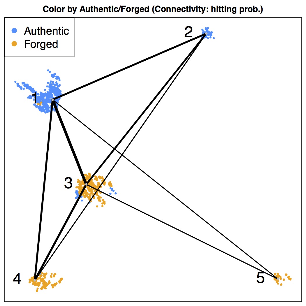
(a) Visualization

	1	2	3	4	5
Authentic	629	70	62	1	0
Forge	4	0	390	179	37

(b) Authentic and Forged currency versus cluster.

	1	2	3	4	5
1	–	0.20	0.30	0.21	0.11
2	0.20	–	0.19	0.12	0.06
3	0.30	0.19	–	0.22	0.12
4	0.21	0.12	0.22	–	0.06
5	0.11	0.06	0.12	0.06	–

(c) Matrix of connectivity

Figure 12: Clustering result for the Bank Authentication data ($d=4$). BlueViolet color is authentic banknote and orange color is the forged banknote. The first two clusters are of the genuine classes while the latter three clusters are the group of forged.

We apply our methods to the banknote authentication data set given in the UCI machine learning database repository (Asuncion and Newman, 2007). The data are extracted from images that are taken from authentic and forged banknote-like specimens and later are digitalized via an industrial camera for print inspection. Each image is a $400\times 400$ pixels gray scale picture with a resolution of about 660 dpi. A wavelet transform is applied to extract features from the images. Each data point contains four attributes: ‘variance of Wavelet Transformed image’, ‘skewness of Wavelet Transformed image’, ‘kurtosis of Wavelet Transformed image’ and ‘entropy of image’.

We apply our methods to analyze this dataset. Note that all clusters are larger than $n_{0}=11.97$ (the smallest cluster has $37$ points) so that we do not filter out any cluster. The following parameters are used:

$$h=0.613,\quad n_{0}=11.97,\quad\rho_{0}=5,\quad\omega_{0}=0.1.$$

The visualization, confusion matrix and matrix of connectivity are given in Figure 12.

From Figure 12, cluster $1$ and $2$ are clusters for the real banknotes while cluster $3,4$ and $5$ are clusters of fake banknotes. By examining the confusion matrix (panel (b)), the cluster $2$ and $5$ are clusters for purely genuine and forged banknote. As can be seen from panel (c), their connectivity is relatively small compared to the other pairs. This suggests that the authentic and fake banknotes are really different in a sense.

8.4 Wine Quality Data

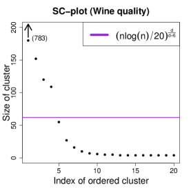
Figure 13: The SC-plot for wine quality data. Our choice of $n_{0}=62.06$ which agrees with the gap between fourth and fifth cluster (containing $109$ and $55$ points).

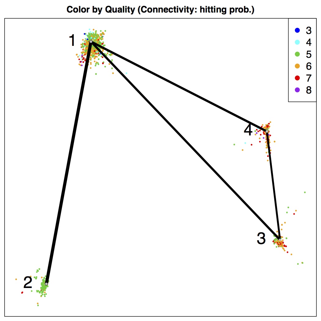
(a) Visualization

Quality	1	2	3	4
3	10	0	0	0
4	49	0	1	3
5	486	135	41	19
6	434	25	91	88
7	68	3	48	80
8	5	0	5	8

(b) Wine quality versus cluster.

	1	2	3	4
1	–	0.33	0.23	0.23
2	0.33	–	0.12	0.12
3	0.23	0.12	–	0.19
4	0.23	0.12	0.19	–

(c) Matrix of connectivity

Figure 14: Clustering result for the Wine Quality data ($d=11$). Color denotes different quality score. The panel (b) shows the components for each cluster so that we can interpret each cluster according to the score distributions. The first cluster is a normal cluster; the second cluster is a cluster of best wines; the third cluster is a ‘better than normal’ cluster while the last cluster is a low-score cluster.

We apply our methods to the wine quality data set given in the UCI machine learning database repository (Asuncion and Newman, 2007). This data set consists of two variants (white and red) of the Portuguese Vinho Verde wine. The detailed information on this data set is given in Cortez et al. (2009). In particular, we focus on the red wine, which consists of $n=1599$ observations. For each wine sample, we have 11 physicochemical measurements: ‘fixed acidity’, ‘volatile acidity’, ‘citric acid’, ‘residual sugar’, ‘chlorides’, ‘free sulfur dioxide’, ‘total sulfur dioxide’, ‘density’, ‘pH’, ‘sulphates’ and ‘alcohol’. Thus, the dimension to this dataset is $d=11$. In addition to the 11physicochemical attributes, we also have one score for each wine sample. This score is evaluated by a minimum of three sensory assessors (using blind tastes), which graded the wine in a scale that ranges from 0 (very bad) to 10 (excellent). The final sensory score is given by the median of these evaluations.

We apply our methods to this dataset using the same reference rules for bandwidth selection and picking $n_{0}$. The SC-plot is given by Figure 13; we notice that the gap occurs at the fourth and fifth clusters and $n_{0}=62.06$ successfully separate these clusters. Note that the first cluster contains $783$ points so that it does not appear in the SC-plot. We measure the connectivity among clusters via the hitting probability method and visualize the data in Figure 14. The following parameters are used in this dataset:

$$h=0.599,\quad n_{0}=62.06,\quad\rho_{0}=5,\quad\omega_{0}=0.125.$$

The wine quality data is very noisy since it involves a human-rating scoring procedure. However, mode clustering suggests that there is structure. From the confusion matrix in Figure 14 panel (b), we find that each cluster can be interpreted in terms of the score distribution. The first cluster is like a ‘normal’ group of wines. It is the largest cluster and the score is normally distributed centering at around $5.5$ (the score $5$ and $6$ are the majority in this cluster). The second cluster is the ‘bad’ group of wines; most of the wines within this cluster have only score $5$. The third and fourth clusters are good clusters; the overall quality within both clusters is high (especially the fourth clusters). Remarkably, the second cluster (bad cluster) does not connect to the third and fourth cluster (good cluster). This shows that our connectivity measure captures some structure.

8.5 Seed Data

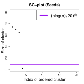
Figure 15: The SC-plot for Seeds data. We pick $n_{0}=8.75$ which filters out the fourth small cluster (compared to the three large clusters).

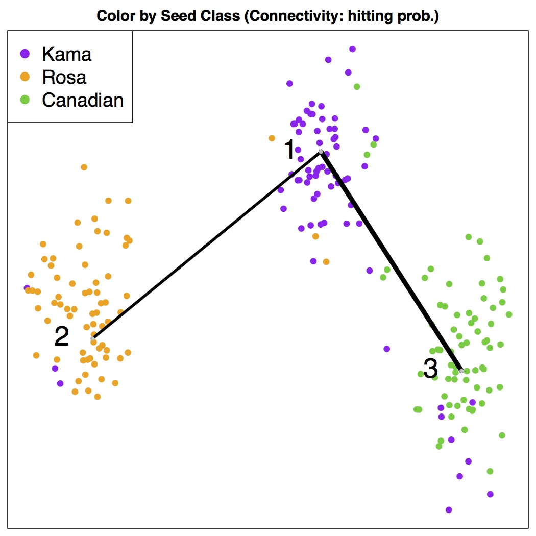
(a) Visualization

Class	1	2	3
Kama	58	3	9
Rosa	3	67	0
Canadian	3	0	67

(b) Seeds class versus cluster.

	1	2	3
1	–	0.18	0.30
2	0.18	–	0.09
3	0.30	0.09	–

(c) Matrix of connectivity

Figure 16: Clustering result for the Seed data ($d=7$). Color denotes different classes of seeds. The three clusters represent three classes of seeds. The fact that the some seeds appear in the wrong cluster is captured by the connectivity measure (the high connection between 1-2 and 1-3).

We apply our methods to the seed data from the UCI machine learning database repository (Asuncion and Newman, 2007). The seed data is contributed by the authors of Charytanowicz et al. (2010). Some preliminary analysis using mode clustering (mean shift) and K-means clustering can be found in Charytanowicz et al. (2010). Scientists examine the kernels from three different variety of wheat: ‘Kama’, ‘Rosa’ and ‘Canadian’; each type of wheat with a randomly selected $70$ sample. For each sample, a soft X-ray technique is conducted to obtain an $13\times 18$ cm image. According to the image, we have 7 attributes ($d=7$): ‘area’, ‘perimeter’, ‘compactness’, ‘length of kernel’, ‘width of kernel’, ‘asymmetry coefficient’ and ‘length of kernel groove’.

We first normalize each attribute and then perform mode clustering according to the bandwidth selected by Silverman’s rule (17). We pick $n_{0}=8.75$ which is reasonable compared with the SC-plot (Figure 15). The visualization, confusion matrix and the matrix of connectivity is given in Figure 16. The following parameters are used in the seeds data

$$h=0.613,\quad n_{0}=8.75,\quad\rho_{0}=5,\quad\omega_{0}=0.167.$$

As can be seen from Figure 16, the three clusters successfully separate the three classes of seeds with little error. The connectivity matrix in panel (c) explains the errors in terms of overlapping of clusters. Some seeds of class ‘Kama’ (corresponding to the third cluster) are in the domain of first and second clusters and we see a higher connectivity among cluster pair 1-2 and 1-3.

8.6 Comparisons

Finally, we compare mode clustering to k-means clustering, spectral clustering and hierarchical clustering for the four real datasets mentioned previously (Olive Oil, Bank Authentication, Wine Quality and Seeds). For the other three methods, we pick the number of clusters as the number of significant clusters by mode clustering. We use a Gaussian kernel for spectral clustering and complete linkage for hierarchical clustering. To compare the quality of clustering, we use the adjusted Rand index (Rand, 1971; Hubert and Arabie, 1985; Vinh et al., 2009). The result is given in Table 17. A higher adjusted rand index indicates a better match clustering result. Note that the adjusted rand index may be negative (e.g. wine quality dataset for spectral clustering and hierarchical clustering). If a negative value occurs, this means that the clustering result is worse than randomly partitioning the data. i.e. the clustering is no better than random guessing.

Dataset/Method	Mode clustering	k-means	Spectral clustering	Hierarchical clustering
Olive Oil	0.826	0.793	0.627	0.621
Bank Authentication	0.559	0.212	0.468	0.062
Wine Quality	0.074	0.034	-0.002	-0.017
Seeds	0.765	0.773	0.732	0.686

Figure 17: Adjusted rand index for each method. Note that the spectral clustering outputs a random result each time due to its implicitly uses of k-means clustering. Here we only display one instance.

From Figure 17, we find that the mode clustering is the best method for the olive oil data, bank authentication dataset, and the wine quality dataset. For the case that mode clustering is suboptimal, the result is still not to far away from the optimal method. On the contrary, k-means is a disaster for the bank authentication dataset and is just a little bit better than mode clustering in the seeds dataset. For the spectral clustering, overall its performance is very good but it fails in the wine quality dataset. The wine quality dataset (Section 8.4) is known to be extremely noisy; this might be the reason why every approach does not give a good result. However, even the noise level is so huge, the mode clustering still detect some hidden structures. See Section 8.4 for more involved discussion.

9 Conclusion

In this paper, we present enhancements to mode clustering methods, including soft mode clustering, a measure of cluster connectivity, a rule for selecting bandwidth, a method for denoising small clusters, and new visualization methods for high-dimensional data. We also establish a ‘standard procedure’ for mode clustering analysis in Figure 7 that can be used to understand the structure of data even in high dimensions. We apply the standard procedure to several examples. The cluster connectivity and visualization methods apply to other clustering methods as well.

Appendix A Appendix: Mixture-Based Soft Clustering

The assignment vector $a(x)$ derived from a mixture model need not be well defined because a density $p$ can have many different mixture representations that can in turn result in distinct soft cluster assignments.

Consider a mixture density

$$p(x)=\sum_{j=1}^{k}\pi_{j}\phi(x;\mu_{j},\Sigma_{j})$$ (27)

where each $\phi(x;\mu_{j},\Sigma_{j})$ is a Gaussian density function with mean $\mu_{j}$ and covariance matrix $\Sigma_{j}$ and $0\leq\pi_{j}\leq 1$ is the mixture proportion for the $j$-th density such that $\sum_{j}\pi_{j}=1$. Recall the latent variable representation of $p$. Let $Z$ be a discrete random variable such that

$$P(Z=j)=\pi_{j},\quad j=1,\cdots,k$$ (28)

and let $X|Z\sim\phi(x;\mu_{Z},\Sigma_{Z})$. Then, consistent with (27), the unconditional density for $X$ is

$$p(x)=\sum_{z}p(x|z)p(z)=\sum_{j=1}\pi_{j}\phi(x;\mu_{j},\Sigma_{j})$$ (29)

It follows that

$$P(Z=j|x)=\frac{\pi_{j}p(x|Z=j)}{\sum_{s=1}\pi_{s}p(x|z=s)}=\frac{\pi_{j}\phi(x;\mu_{j},\Sigma_{j})}{\sum_{s=1}\pi_{s}\phi(x;\mu_{s},\Sigma_{s})},$$ (30)

with soft cluster assignment $a(x)=(a_{1}(x),\cdots,a_{k}(x))=(p(z=1|x),\cdots,p(z=k|x))$. Of course, $a(x)$ can be estimated from the data by estimating the parameters of the mixture model.

We claim that the $a(x)$ is not well-defined. Consider the following example in one dimension. Let

$$p(x)=\frac{1}{2}\phi(x;-3,1)+\frac{1}{2}\phi(x;3,1).$$ (31)

Then by definition

$$a_{1}(x)=P(Z=1|x)=\frac{\frac{1}{2}\phi(x;-3,1)}{\frac{1}{2}\phi(x;-3,1)+\frac{1}{2}\phi(x;3,1)}.$$ (32)

However, we can introduce a different latent variable representation for $p(x)$ as follows. Let us define

$$p_{1}(x)=\frac{p(x)1(x\leq 4)}{\int p(x)1(x\leq 4)dx}$$ (33)

and

$$p_{2}(x)=\frac{p(x)1(x>4)}{\int p(x)1(x>4)dx}$$ (34)

and note that

$$p(x)=\pi p_{1}(x)+(1-\pi)p_{2}(x)$$ (35)

where $\pi=\int p(x)1(x\leq 4)dx$. Here, $1(E)$ is the indicator function for $E$. Let $W$ be a discrete random variable such that $P(W=1)=\pi$ and $P(W=2)=1-\pi$ and let $X|W$ has density $p_{W}(x)$. Then we have $p(x)=\sum_{w}p(x|w)P(W=w)$ which is the same density as (31). This defined the soft clustering assignment $a(x)=(P(W=1|x),\cdots,P(W=k|x))$ where

$$a_{1}(x)=P(W=1|x)=1(x\leq 4)$$ (36)

which is completely different from (32). In fact, for any set $A\subset\mathbb{R}$, there exists a latent representation of $p(x)$ such that $a_{1}(x)=I(x\in A)$. There are infinitely many latent variable representations for any density, each leading to a different soft clustering. The mixture-based soft clustering thus depends on the arbitrary, chosen representation.

Appendix B Appendix: Proofs

Proof of Theorem 1.

For two vector-value functions $f(x),g(x)\in\mathbb{R}^{d}$ and two matrix-value functions $A(x),B(x)\in\mathbb{R}^{d_{1}\times d_{2}}$, we define the ${\cal L}^{\infty}$ norms

$$\|f-g\|_{\max,\infty}=\sup_{x}\|f(x)-g(x)\|_{\max},\qquad\|A-B\|_{\max,\infty}=\sup_{x}\|A(x)-B(x)\|_{\max},$$ (37)

where $\|f(x)-g(x)\|_{\max},\|A(x)-B(x)\|_{\max}$ are the elementwise maximal norm. Similarly, for two scalar-value functions $p(x),q(x)$, $\|p-q\|_{\infty}=\sup_{x}|p(x)-q(x)|$ is the ordinary ${\cal L}^{\infty}$ norm.

Modal consistency: Our proof consists of three steps. First, we show that when $p,\widehat{p}_{n}$ are sufficiently close, each local modes $m_{j}$ corresponds to a unique $\widehat{m}_{j}$. Second, we show that when $\|\nabla p-\nabla\widehat{p}_{n}\|_{\max,\infty}$ and $\|\nabla\nabla p-\nabla\nabla\widehat{p}_{n}\|_{\max,\infty}$ are small, all the estimated local mode must be near to some local modes. The first two steps and (M2) construct a condition for an unique 1-1 correspondence between elements of $\mathcal{M}$ and $\widehat{\mathcal{M}}_{n}$. The last step is to apply Talagrand’s inequality to get the exponential bound for the probability of the desire condition.

Step 1: WLOG, we consider a local mode $m_{j}$. Now we consider the set

$$S_{j}=m_{j}\oplus\frac{\lambda_{*}}{2dC_{3}}.$$

Since the third derivative of $p$ is bounded by $C_{3}$,

$$\sup_{x\in S_{j}}\|\nabla\nabla p(m_{j})-\nabla\nabla p(x)\|_{\max}\leq\frac{\lambda_{*}}{2dC_{3}}\times C_{3}=\frac{\lambda_{*}}{2d}.$$

Thus, by Weyl’s theorem (Theorem 4.3.1 in Horn and Johnson (2013)) and condition (M1), the first eigenvalue is bounded by

$$\sup_{x\in S_{j}}\lambda_{1}(x)\leq\lambda_{1}(m_{j})+d\times\frac{\lambda_{*}}{2d}\leq-\frac{\lambda_{*}}{2}.$$ (38)

Note that eigenvalues at local modes are negative. Since $\nabla p(m_{j})=0$ and the eigenvalues are bounded around $m_{j}$, the density at the boundary of $S_{j}$ must be less than

$$\sup_{x\in\partial S_{j}}p(x)\leq p(m_{j})-\frac{1}{2}\frac{\lambda_{*}}{2}\left(\frac{\lambda_{*}}{2dC_{3}}\right)^{2}=p(m_{j})-\frac{\lambda_{*}^{3}}{16d^{2}C_{3}^{2}},$$

where $\partial S_{j}=\{x:\|x-m_{j}\|=\frac{\lambda_{*}}{2dC_{3}}\}$ is the boundary of $S_{j}$. Thus, whenever

$$\|\widehat{p}_{n}-p\|_{\infty}<\frac{\lambda_{*}^{3}}{16d^{2}C_{3}^{2}},$$ (39)

there must be at least one estimated local mode $\widehat{m}_{j}$ within $S_{j}=m\oplus\frac{\lambda_{*}}{2dC_{3}}$. Note that this can be generalized to each $j=1,\cdots,k$.

Step 2: It is straightforward to see that whenever

$$\|\nabla\widehat{p}_{n}-\nabla p\|_{\max,\infty} \leq\eta_{1},$$ (40)

$$\|\nabla\nabla\widehat{p}_{n}-\nabla\nabla p\|_{\max,\infty} \leq\frac{\lambda_{*}}{4d},$$

the estimated local modes

$$\widehat{\mathcal{M}}_{n}\subset\mathcal{M}\oplus\frac{\lambda_{*}}{2dC_{3}}$$

by using (M2), triangular inequality and again Weyl’s theorem for the eigenvalues.

Step 3: By Step 1 and 2,

$$\widehat{\mathcal{M}}_{n}\subset\mathcal{M}\oplus\frac{\lambda_{*}}{2dC_{3}}$$

and for each mode $m_{j}$ there exists at least one estimated mode $\widehat{m}_{j}$ within $S_{j}=m_{j}\oplus\frac{\lambda_{*}}{2dC_{3}}$. Now apply (38) and second inequality of (40) and triangular inequality, we conclude

$$\sup_{x\in S_{j}}\widehat{\lambda}_{1}(x)\leq-\frac{\lambda_{*}}{4},$$ (41)

where $\widehat{\lambda}_{1}(x)$ is the first eigenvalue of $\nabla\nabla\widehat{p}_{n}(x)$. This shows that we cannot have two estimated local modes within each $S_{j}$. Thus, each $m_{j}$ only corresponds to one $\widehat{m}_{j}$ and vice versa by Step 2. We conclude that a sufficient condition for the number of modes being the same is the inequality required in (39) and (40) i.e. we need

$$\|\widehat{p}_{n}-p\|_{\infty} <\frac{\lambda_{*}^{3}}{16d^{2}C_{3}^{2}},$$ (42)

$$\|\nabla\widehat{p}_{n}-\nabla p\|_{\max,\infty} \leq\eta_{1},$$

$$\|\nabla\nabla\widehat{p}_{n}-\nabla\nabla p\|_{\max,\infty} \leq\frac{\lambda_{*}}{4d}.$$

Let $p_{h}=\mathbb{E}(\widehat{p}_{n})$ be the smoothed version of the KDE. It is well-known in nonparametric theory that (see e.g. page 132 in Scott (2009))

$$\|p_{h}-p\|_{\infty} =O(h^{2}),$$ (43)

$$\|\nabla p_{h}-\nabla p\|_{\max,\infty} =O(h^{2}),$$

$$\|\nabla\nabla p_{h}-\nabla\nabla p\|_{\max,\infty} =O(h^{2}).$$

Thus, as $h$ is sufficiently small, we have

$$\|p_{h}-p\|_{\infty}<\frac{\lambda_{*}^{3}}{32d^{2}C_{3}^{2}},\qquad\|\nabla p_{h}-\nabla p\|_{\max,\infty}\leq\eta_{1}/2,\qquad\|\nabla\nabla p_{h}-\nabla\nabla p\|_{\max,\infty}\leq\frac{\lambda_{*}}{8d}.$$ (44)

Thus, (42) holds whenever

$$\|\widehat{p}_{n}-p_{h}\|_{\infty} <\frac{\lambda_{*}^{3}}{32d^{2}C_{3}^{2}},$$ (45)

$$\|\nabla\widehat{p}_{n}-\nabla p_{h}\|_{\max,\infty} \leq\eta_{1}/2,$$

$$\|\nabla\nabla\widehat{p}_{n}-\nabla\nabla p_{h}\|_{\max,\infty} \leq\frac{\lambda_{*}}{8d}$$

and $h$ is sufficiently small.

Now applying Talagrand’s inequality (Talagrand, 1996; Gine and Guillou, 2002) (see also equation (90) in Lemma 13 in Chen et al. (2014b) for a similar result), there exists constants $A_{0},A_{1},A_{2}$ and $B_{0},B_{1},B_{2}$ such that for $n$ sufficiently large,

$$\mathbf{P}\left(\|\widehat{p}_{n}-p_{h}\|_{\infty}\geq\epsilon\right) \leq B_{0}e^{-A_{0}\epsilon nh^{d}},$$ (46)

$$\mathbf{P}\left(\|\nabla\widehat{p}_{n}-\nabla p_{h}\|_{\max,\infty}\geq\epsilon\right) \leq B_{1}e^{-A_{1}\epsilon nh^{d+2}},$$

$$\mathbf{P}\left(\|\nabla\nabla\widehat{p}_{n}-\nabla\nabla p_{h}\|_{\max,\infty}\geq\epsilon\right) \leq B_{2}e^{-A_{2}\epsilon nh^{d+4}}.$$

Thus, combining (45) and (46), we conclude that there exists some constants $A_{3},B_{3}$ such that

$$\mathbb{P}(\eqref{eq::pf1_5}\mbox{ holds})\geq 1-B_{3}e^{-A_{3}nh^{d+4}}$$ (47)

when $h$ is sufficiently small. Since (42) holds implies $\widehat{k}_{n}=k$, we conclude

$$\mathbb{P}(\widehat{k}_{n}\neq k)\leq B_{3}e^{-A_{3}nh^{d+4}}$$ (48)

for some constants $B_{3},A_{3}$ as $h$ is sufficiently small. This proves modal consistency.

Location convergence: For the location convergence, we assume (42) holds so that $\widehat{k}_{n}=k$ and each local mode is approximating by an unique estimated local mode. We focus on one local mode $m_{j}$ and derive the rate of convergence for $\|\widehat{m}_{j}-m_{j}\|$ and then generalized this rate to all the local modes.

By definition,

$$\nabla p(m_{j})=\nabla\widehat{p}_{n}(\widehat{m}_{j})=0.$$

Thus, by Taylor expansion and the fact that the third derivative of $\widehat{p}_{n}$ is uniformly bounded,

$$\nabla\widehat{p}_{n}(m_{j}) =\nabla\widehat{p}_{n}(\widehat{m}_{j})-\nabla\widehat{p}_{n}(m_{j})$$ (49)

$$=\nabla\nabla\widehat{p}_{n}(m_{j})(\widehat{m}_{j}-m_{j})+o(\|\widehat{m}_{j}-m_{j}\|).$$

Since we assume (42), this implies all eigenvalues of $\nabla\nabla\widehat{p}_{n}(m_{j})$ are bounded away from $0$ so that $\nabla\nabla\widehat{p}_{n}(m_{j})$ is invertible. Moreover,

$$\nabla\widehat{p}_{n}(m_{j}) =\nabla\widehat{p}_{n}(m_{j})-\nabla p(m_{j})$$ (50)

$$=O(h^{2})+O_{P}\left(\sqrt{\frac{1}{nh^{d+2}}}\right)$$

by the rate of pointwise convergence in nonparametric theory (see e.g. page 154 in Scott (2009)). Thus, we conclude

$$\|\widehat{m}_{j}-m_{j}\|=O(h^{2})+O_{P}\left(\sqrt{\frac{1}{nh^{d+2}}}\right).$$ (51)

Now applying this rate of convergence to each local mode and use the fact that

$${\sf Haus}\left(\widehat{\mathcal{M}}_{n},\mathcal{M}\right)=\max_{j=1,\cdots,k}\|\widehat{m}_{j}-m_{j}\|,$$

we conclude the rate of convergence for estimating the location.

$\square$

—

References

- Arias-Castro et al. (2013) E. Arias-Castro, D. Mason, and B. Pelletier. On the estimation of the gradient lines of a density and the consistency of the mean-shift algoithm. Technical report, IRMAR, 2013.
- Asuncion and Newman (2007) A. Asuncion and D. Newman. Uci machine learning repository, 2007.
- Azzalini and Torelli (2007) A. Azzalini and N. Torelli. Clustering via nonparametric density estimation. Statistics and Computing, 17(1):71–80, 2007. ISSN 0960-3174. 10.1007/s11222-006-9010-y.
- Banyaga (2004) A. Banyaga. Lectures on Morse homology, volume 29. Springer Science & Business Media, 2004.
- Chacon (2014) J. Chacon. A population background for nonparametric density-based clustering. arXiv:1408.1381, 2014.
- Chacón and Duong (2013) J. Chacón and T. Duong. Data-driven density derivative estimation, with applications to nonparametric clustering and bump hunting. Electronic Journal of Statistics, 2013.
- Chacón et al. (2011) J. Chacón, T. Duong, and M. Wand. Asymptotics for general multivariate kernel density derivative estimators. Statistica Sinica, 2011.
- Chacón (2012) J. E. Chacón. Clusters and water flows: a novel approach to modal clustering through morse theory. arXiv preprint arXiv:1212.1384, 2012.
- Charytanowicz et al. (2010) M. Charytanowicz, J. Niewczas, P. Kulczycki, P. A. Kowalski, S. Łukasik, and S. Żak. Complete gradient clustering algorithm for features analysis of x-ray images. In Information Technologies in Biomedicine, pages 15–24. Springer, New York, NY, USA NY, 2010.
- Chaudhuri and Dasgupta (2010) K. Chaudhuri and S. Dasgupta. Rates of convergence for the cluster tree. NIPS, 2010.
- Chazal et al. (2011) F. Chazal, L. Guibas, S. Oudot, and P. Skraba. Persistence-based clustering in riemannian manifolds. In Proceedings of the 27th annual ACM symposium on Computational geometry, pages 97–106. ACM, 2011.
- Chazal et al. (2014) F. Chazal, B. T. Fasy, F. Lecci, B. Michel, A. Rinaldo, and L. Wasserman. Robust topological inference: Distance to a measure and kernel distance. arXiv preprint arXiv:1412.7197, 2014.
- Chen et al. (2014a) Y.-C. Chen, C. R. Genovese, R. J. Tibshirani, and L. Wasserman. Nonparametric modal regression. arXiv preprint arXiv:1412.1716, 2014a.
- Chen et al. (2014b) Y.-C. Chen, C. R. Genovese, and L. Wasserman. Asymptotic theory for density ridges. arXiv: 1406.5663, 2014b.
- Chen et al. (2014c) Y.-C. Chen, C. R. Genovese, and L. Wasserman. Generalized mode and ridge estimation. arXiv: 1406.1803, 2014c.
- Cheng (1995) Y. Cheng. Mean shift, mode seeking, and clustering. Pattern Analysis and Machine Intelligence, IEEE Transactions on, 17(8):790–799, 1995.
- Comaniciu and Meer (2002) D. Comaniciu and P. Meer. Mean shift: a robust approach toward feature space analysis. Pattern Analysis and Machine Intelligence, IEEE Transactions on, 24(5):603 –619, may 2002.
- Cortez et al. (2009) P. Cortez, A. Cerdeira, F. Almeida, T. Matos, and J. Reis. Modeling wine preferences by data mining from physicochemical properties. Decision Support Systems, 47(4):547–553, 2009.
- De Silva and Tenenbaum (2004) V. De Silva and J. B. Tenenbaum. Sparse multidimensional scaling using landmark points. Technical report, Technical report, Stanford University, 2004.
- Einmahl and Mason (2005) U. Einmahl and D. M. Mason. Uniform in bandwidth consistency for kernel-type function estimators. The Annals of Statistics, 2005.
- Fasy et al. (2014) B. T. Fasy, F. Lecci, A. Rinaldo, L. Wasserman, S. Balakrishnan, and A. Singh. Statistical inference for persistent homology: Confidence sets for persistence diagrams. The Annals of Statistics, 2014.
- Forina et al. (1983) M. Forina, C. Armanino, S. Lanteri, and E. Tiscornia. Classification of olive oils from their fatty acid composition. Food Research and Data Analysis, 1983.
- Fukunaga and Hostetler (1975) K. Fukunaga and L. D. Hostetler. The estimation of the gradient of a density function, with applications in pattern recognition. IEEE Transactions on Information Theory, 21:32–40, 1975.
- Genovese et al. (2009) C. R. Genovese, M. Perone-Pacifico, I. Verdinelli, L. Wasserman, et al. On the path density of a gradient field. The Annals of Statistics, 37(6A):3236–3271, 2009.
- Genovese et al. (2012) C. R. Genovese, M. Perone-Pacifico, I. Verdinelli, and L. Wasserman. Nonparametric ridge estimation. arXiv:1212.5156v1, 2012.
- Gine and Guillou (2002) E. Gine and A. Guillou. Rates of strong uniform consistency for multivariate kernel density estimators. In Annales de l’Institut Henri Poincare (B) Probability and Statistics, 2002.
- Guest (2001) M. A. Guest. Morse theory in the 1990’s. arXiv:math/0104155v1, 2001.
- Hartigan (1975) J. Hartigan. Clustering Algorithms. Wiley and Sons, Hoboken, NJ, 1975.
- Hastie et al. (2001) T. Hastie, R. Tibshirani, and J. Friedman. The Elements of Statistical Learning. Springer Series in Statistics. Springer New York Inc., New York, NY, USA, 2001.
- Horn and Johnson (2013) R. A. Horn and C. R. Johnson. Matrix Analysis. Cambridge, second edition, 2013.
- Hubert and Arabie (1985) L. Hubert and P. Arabie. Comparing partitions. Journal of classification, 2(1):193–218, 1985.
- Kpotufe and von Luxburg (2011) S. Kpotufe and U. von Luxburg. Pruning nearest neighbor cluster trees. arXiv preprint arXiv:1105.0540, 2011.
- Li et al. (2007) J. Li, S. Ray, and B. Lindsay. A nonparametric statistical approach to clustering via mode identification. Journal of Machine Learning Research, 8(8):1687–1723, 2007.
- Lingras and West (2002) P. Lingras and C. West. Interval set clustering of web users with rough k-means. Journal of Intelligent Information Systems, 2002.
- McLachlan and Peel (2004) G. McLachlan and D. Peel. Finite mixture models. John Wiley & Sons, Hoboken, NJ, 2004.
- Morse (1925) M. Morse. Relations between the critical points of a real function of n independent variables. Transactions of the American Mathematical Society, 27(3):345–396, 1925.
- Morse (1930) M. Morse. The foundations of a theory of the calculus of variations in the large in m-space (second paper). Transactions of the American Mathematical Society, 32(4):599–631, 1930.
- Nock and Nielsen (2006) R. Nock and F. Nielsen. On weighting clustering. IEEE Transactions on Pattern Analysis and Machine Intelligence, 2006.
- Peters et al. (2013) G. Peters, F. Crespoc, P. Lingrasd, and R. Weber. Soft clustering - fuzzy and rough approaches and their extensions and derivatives. International Journal of Approximate Reasoning, 2013.
- Pollard (1985) D. Pollard. New ways to prove central limit theorems. Econometric Theory, 1985.
- Rand (1971) W. M. Rand. Objective criteria for the evaluation of clustering methods. Journal of the American Statistical association, 66(336):846–850, 1971.
- Romano (1988) J. P. Romano. Bootstrapping the mode. Annals of the Institute of Statistical Mathematics, 40(3):565–586, 1988.
- Romano et al. (1988) J. P. Romano et al. On weak convergence and optimality of kernel density estimates of the mode. The Annals of Statistics, 16(2):629–647, 1988.
- Scott (2009) D. W. Scott. Multivariate density estimation: theory, practice, and visualization, volume 383. John Wiley & Sons, 2009.
- Sheather (2004) S. J. Sheather. Density estimation. Statistical Science, 2004.
- Silva and Tenenbaum (2002) V. D. Silva and J. B. Tenenbaum. Global versus local methods in nonlinear dimensionality reduction. In Advances in neural information processing systems, pages 705–712, 2002.
- Stuetzle (2003) W. Stuetzle. Estimating the cluster tree of a density by analyzing the minimal spanning tree of a sample. Journal of Classification, 20(1):025–047, 2003. ISSN 0176-4268. 10.1007/s00357-003-0004-6. URL http://dx.doi.org/10.1007/s00357-003-0004-6.
- Talagrand (1996) M. Talagrand. Newconcentration inequalities in product spaces. Invent. Math, 1996.
- Vinh et al. (2009) N. X. Vinh, J. Epps, and J. Bailey. Information theoretic measures for clusterings comparison: is a correction for chance necessary? In Proceedings of the 26th Annual International Conference on Machine Learning, pages 1073–1080. ACM, 2009.
—