Minimum correlation for any bivariate Geometric distribution

Abstract.

Consider a bivariate Geometric random variable where the first component has parameter $p_{1}$ and the second parameter $p_{2}$. It is not possible to make the correlation between the marginals equal to -1. Here the properties of this minimum correlation are studied both numerically and analytically. It is shown that the minimum correlation can be computed exactly in time $O(p_{1}^{-1}\ln(p_{2}^{-1})+p_{2}^{-1}\ln(p_{1}^{-1}))$. One method for generating a bivariate geometric with target correlation requires computing this minimum correlation. The minimum correlation is shown to be nonmonotonic in $p_{1}$ and $p_{2}$, moreover, the partial derivatives are not continuous. For $p_{1}=p_{2}$, these discontinuities are characterized completely and shown to lie near (1 - roots of 1/2). In addition, we construct analytical bounds on the minimum correlation.

1. Introduction

We investigate the minimum attainable correlation between two Geometric random variables. Most students graduate believing that any correlation in $[-1,1]$ is attainable by a bivariate distribution. That, of course, is not true, except for distributions with symmetric support like Normal and Uniform (see Moran (1967)). The consequence is that, in data analysis, empirical correlation is often misinterpreted, and compared to $-1$ and $1$ instead to the theoretical bounds. See Denuit and Dhaene (2003) and Shih and Huang (1992) for a discussion. Therefore, attainable correlation is crucial information about a multivariate distribution. Still, there is much more unknown than known facts in this field, especially in higher dimensions. In bivariate case, minimum correlation for several important distributional examples is analyzed in Conway (1979) and Dukic and Marić (2013) (and references therein). The purpose of the present paper is to fill the gap in this subject concerning one of the most important discrete cases–the Geometric distribution.

Say that $X$ has a Geometric distribution with parameter $p$ ($0<p\leq 1$) and write $X\sim\textsf{Geo}(p)$, if for all $i\in\{0,1,2,\ldots\}$, $\mathbb{P}(X=i)=p(1-p)^{i}$. If one has a coin with probability $p$ of heads, then $X\sim\textsf{Geo}(p)$ represents the number of tails flipped before obtaining a heads.

For $(p_{1},p_{2})\in(0,1]^{2}$, let

$$\rho_{-}(p_{1},p_{2})=\min\{\operatorname{Corr}(X_{1},X_{2}):X_{1}\sim\textsf{Geo}(p_{1}),X_{2}\sim\textsf{Geo}(p_{2})\}.$$

When $p_{1}=p_{2}=p$, Figure 1.1 shows a graph of this minimum correlation as a function of $p$. Several properties are immediately apparent. First, the correlation is not a monotonic function of $p$. In addition, there are points of discontinuity in the derivative of the graph. These phenomena are explained in Section 3.

In Section 2 it is shown that the value of $\rho_{-}(p_{1},p_{2})$ can be found exactly in time $O(p_{1}^{-1}\ln(p_{1}^{-1})+p_{2}^{-1}\ln(p_{2}^{-1}))$. In addition, upper and lower bounds for this function are computed.

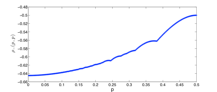
Figure 1.1. The minimum correlation $\rho_{-}(p,p)$ for $p<1/2$. When $p\geq 1/2$ the minimum correlation is simply equal to $p-1$.

To understand $\rho_{-}$, first consider the inverse transform method for generating a random variate with a specified cdf (cumulative distribution function) $F$. Define the pseudoinverse of the cdf as

$$F^{-1}(u)=\inf\{x:F(x)\geq u\}.$$ (1.1)

When $U$ is uniform over the interval $[0,1]$ (write $U\sim\textsf{Unif}([0,1])$), $F^{-1}(U)$ is a random variable with cdf $F$ (see for instance p. 28 of Devroye (1986)). Since $U$ and $1-U$ have the same distribution, both can be used in the inverse transform method. The random variables $U$ and $1-U$ are antithetic random variables.

We will use the notation $X\sim Y$ when $X$ has the same probability distribution as $Y$. The following result comes from work of Fréchet (1951) and Hoeffding (1940).

Lemma 1.1 (Fréchet-Hoeffding bound).

For $X_{1}$ with cdf $F_{1}$ and $X_{2}$ with cdf $F_{2}$, and $U\sim\textsf{Unif}([0,1])$:

$$\operatorname{Corr}(F_{1}^{-1}(U),F_{2}^{-1}(1-U))\leq\operatorname{Corr}(X_{1},X_{2})\leq\operatorname{Corr}(F_{1}^{-1}(U),F_{2}^{-1}(U)).$$

Conversely, if $\operatorname{Corr}(X_{1},X_{2})$ equals the minimum correlation then it holds that $(X_{1},X_{2})\sim(F_{1}^{-1}(U),F_{2}^{-1}(1-U))$. For correlation equal to the maximum value, $(X_{1},X_{2})\sim(F_{1}^{-1}(U),F_{2}^{-1}(U))$.

In other words, the maximum correlation between $X_{1}$ and $X_{2}$ is achieved when the same uniform is used in the inverse transform method to generate both. The minimum correlation between $X_{1}$ and $X_{2}$ is achieved when antithetic random variates are used in the inverse transform method. In the literature on dependence and copulas (see for instance Nelsen, 2006 and Denuit and Dhaene, 2003) $(F_{1}^{-1}(U),F_{2}^{-1}(U))$ and $(F_{1}^{-1}(U),F_{2}^{-1}(1-U))$ are known as the comonotonic and countermonotonic vectors, respectively.

For $X\sim\textsf{Geo}(p)$, the expectation and variance are well known: $\mathbb{E}(X)=(1-p)/p$ and $\mathbb{V}(X)=(1-p)/p^{2}$. The cdf is

$$F_{p}(a)=\mathbb{P}(X\leq a)=p+p(1-p)+\cdots p(1-p)^{a}=1-(1-p)^{a+1}.$$

Lemma 1.2.

The pseudoinverse $F_{p}^{-1}$ of $F_{p}$ is

$$F_{p}^{-1}(u)=\sum_{n=1}^{\infty}\mathbf{1}(1-(1-p)^{n}\leq u<1-(1-p)^{n+1}).$$

[Here $\mathbf{1}(\text{expression})$ is the indicator function that evaluates to 1 when the Boolean expression in the argument is true, and is 0 otherwise.]

Proof.

As the cdf of $X$ is $1-(1-p)^{a+1}$, for $u\in[1-(1-p)^{n}\leq u<1-(1-p)^{n+1}]$, it holds that $\mathbb{P}(X\leq n)\geq u$ and $\mathbb{P}(X\leq n-1)<u$. ∎

Prior Work

Several authors have studied the construction of bivariate geometric distributions. Downton (1970) created such a distribution as a means to create a bivariate exponential for reliability applications where two processes are receiving shocks in a memoryless correlated fashion. Hawkes (1972) generalized Downton’s family as follows. Consider a bivariate Bernoulli distribution $(A,B)$ where for all $i$ and $j$ in $\{0,1\}$:

$$\mathbb{P}(A=i,B=j)=p_{ij}.$$

Then if $(A_{i},B_{i})$ are an iid sequence of draws from this distribution for $i\in\{1,2,3,\ldots\}$, let $X_{1}=\min\{i:A_{i+1}=1\}$, $X_{2}=\min\{i:B_{i+1}=1\}$. It is easy to show that this gives $X_{1}\sim\textsf{Geo}(p_{10}+p_{11}),$ $X_{2}\sim\textsf{Geo}(p_{01}+p_{11})$.

Marshall and Olkin (1985) then showed that the geometrics obtained in this fashion have a minimum correlation of at least $-1/4$.

Paulson and Uppuluri (1972) built a bivariate distribution by taking advantage of a recursive formulation of the geometric from Uppuluri et al. (1967). They do not analyze the minimum correlation, only showing that their family of distributions is not rich enough to include the case that the components are independent.

In Dukic and Marić (2013) (and see also Huber and Marić, 2015), it is shown how to simulate a bivariate Geometric distribution that attains any value between the maximum and minimum correlation, although these methods require knowledge of the maximum and minimum correlation.

Therefore our first main result concerns computation of the minimum correlation. Since the bivariate geometric distribution has infinite support, it is important to note the minimum correlation can be computed relatively quickly.

Theorem 1.3.

The minimum correlation between $X_{1}\sim\textsf{Geo}(p_{1})$ and $X_{2}\sim\textsf{Geo}(p_{2})$ can be computed in time $O(p_{1}^{-1}\ln(p_{2}^{-1})+p_{2}^{-1}\ln(p_{1}^{-1}))$.

Our second main result is a proof of certain properties of the function $\rho_{-}(p,p)$.

Theorem 1.4.

Let $\rho_{-}(p)$ be the minimum correlation achieved between $X_{1}$ and $X_{2}$ where both are $\textsf{Geo}(p)$. Then the following is true.

1. There is an infinite number of points where $(d/dp)\rho_{-}(p)$ is discontinuous.

2. The points where the discontinuities occur are near to $(1$ - roots of $1/2)$.

3. The function is upper and lower bounded by:

   $$g(p)-p\leq\rho_{-}(p)\leq g(p)$$

   where

   $$g(p)=\frac{p^{2}}{[\ln(1-p)]^{2}}\cdot\frac{1}{1-p}\left(2-\frac{\pi^{2}}{6}\right)-(1-p).$$

To bound $\operatorname{Corr}(F_{p}^{-1}(U),F_{p}^{-1}(1-U))$, the minimum correlation, the key is computing $\mathbb{E}(F_{p}^{-1}(U)F_{p}^{-1}(1-U))$. Section 2 looks at finding this quantity for various values of $p$. Some computational details are left for the Appendix, Section 5. Section 3 then proves an upper and lower bound on the $\rho_{-}(p)$ function, as well as the asymptotic behavior of the “bumps” in the function.

2. Computing the minimum correlation

For simplicity consider first the case that $p=p_{1}=p_{2}$.

For any bivariate random variables with the same marginal distributions, the maximum correlation is always 1. More interesting is the minimum correlation. For geometric marginals, the minimum correlation is markedly different when $p<1/2$ and when $p\geq 1/2$.

Lemma 2.1.

Let $\rho_{-}(p)$ be the minimum correlation achievable between $X_{1}$ and $X_{2}$ where both are $\textsf{Geo}(p)$. It is possible to compute $\rho_{-}(p)$ in $O(p^{-1}\ln(p^{-1}))$ steps.

Proof.

As in the introduction, let $U\sim\textsf{Unif}([0,1])$, $X_{1}=F_{p}^{-1}(U)$ and $X_{2}=F_{p}^{-1}(1-U).$

$\bullet$ Consider the $p\geq 1/2$ case. Then either $U$ or $1-U$ falls in the interval $[0,p]$ so either $X_{1}$ or $X_{2}$ is 0. Hence $\mathbb{E}(F_{p}^{-1}(U)F^{-1}_{p}(1-U))=0$ and

$$\rho_{-}(p)=\frac{0-[(1-p)/p]^{2}}{(1-p)/p^{2}}=p-1.$$

$\bullet$ Next suppose $p<1/2$. As in the $p\geq 1/2$ case, if either $U$ or $1-U$ falls in $[0,p]$, then $X_{1}X_{2}=0$ and so consider when $U\in[p,1-p]$.

Let $q=1-p$, $\alpha_{i}=1-q^{i}$, and $\beta_{i}=q^{i}$. With this notation, $F_{p}(i)=\alpha_{i+1}$, and the pseudoinverse becomes

$$F^{-1}_{p}(u)=\sum_{i=1}^{\infty}\mathbf{1}(U\in[\alpha_{i},\alpha_{i+1})).$$

Note that

$$p=\alpha_{1}<\alpha_{2}<\cdots<\alpha_{c}\leq 1-p,$$

where $c=\lfloor\ln(p)/\ln(1-p)\rfloor=\lfloor\log_{1-p}(p)\rfloor.$

When $U\in[\alpha_{i},\alpha_{i+1})$, $X_{1}=i$. At the same time, when $1-U\in[\alpha_{i},\alpha_{i+1})$, $X_{2}=i$. Hence there are at most $2c$ breakpoints changing the value of $X_{1}$ or $X_{2}$. Therefore there are at most $2c$ different values of $(X_{1},X_{2})$ where one of the variables is not 0. This makes it possible to compute $\mathbb{E}(X_{1}X_{2})$ in $O(c)=O(p^{-1}\ln(p^{-1}))$ time. For more details see the Appendix. ∎

Example: ${\mathbf{p=1/4}}$

As an example of how this can be used to calculate the minimum correlation, consider the case when $p=1/4$.

Here $c=\lfloor\ln(1/4)/\ln(3/4)\rfloor=4$, and so the $\alpha_{i}$ and $\beta_{i}$ values for interval $[1/4,3/4]$ become

	$i$
	1	2	3	4
$\alpha_{i}$	$1/4=64/256$	$112/256$	$148/256$	$175/256$
$\beta_{i}$	$3/4=192/256$	$144/256$	$108/256$	$81/256$

Ordering the $\alpha_{i}$ and $\beta_{i}$ divides $[1/4,3/4]$ into seven pieces:

$$(x_{1},x_{2},\ldots,x_{8})=\left(\frac{65}{256},\frac{81}{256},\frac{108}{256},\frac{112}{256},\frac{144}{256},\frac{148}{256},\frac{175}{256},\frac{192}{256}\right).$$

The seven intervals are then

Interval	$[x_{1},x_{2}]$	$[x_{2},x_{3}]$	$[x_{3},x_{4}]$	$[x_{5},x_{6}]$	$[x_{6},x_{7}]$	$[x_{1},x_{2}]$	$[x_{1},x_{2}]$
$(X_{1},X_{2})$	$(1,4)$	$(1,3)$	$(1,2)$	$(2,2)$	$(2,1)$	$(3,1)$	$(4,1)$

Hence

$$\mathbb{E}(X_{1}X_{2})=1\cdot 4\cdot\frac{81-65}{256}+1\cdot 3\cdot\frac{108-81}{256}+\cdots+4\cdot 1\cdot\frac{192-175}{256}=\frac{442}{256}\approx 1.7266,$$

which gives a minimum correlation of $\rho_{-}(1/4)=-1862/3072=-0.606.$

Lemma 2.2.

Let $\rho_{-}(p_{1},p_{2})$ be the minimum correlation achievable between $X_{1}\sim\textsf{Geo}(p_{1})$ and $X_{2}\sim\textsf{Geo}(p_{2})$. Then it is possible to compute $\rho_{-}(p_{1},p_{2})$ in $O(p_{1}^{-1}\ln(p_{2}^{-1})+p_{2}^{-1}\ln(p_{1}^{-1}))$ steps.

Proof.

The proof is essentially the same as for the previous lemma. Since $\mathbb{E}[X_{1}]$, $\mathbb{E}[X_{2}]$, $\mathbb{V}(X_{1})$, and $\mathbb{V}(X_{2})$ are easy to calculate, the difficult part is finding $\mathbb{E}[X_{1}X_{2}]$ using antithetic random variables.

Let $\chi_{1}(u)=\lfloor\log_{1-p_{1}}(1-u)\rfloor$ and $\chi_{2}(u)=\lfloor\log_{1-p_{2}}(u)\rfloor$ for $u\in[0,1]$. Then note $X_{1}=\chi_{1}(U)$ and $X_{2}=\chi_{2}(U)$, so

$$\mathbb{E}[X_{1}X_{2}]=\int_{0}^{1}\chi_{1}(u)\chi_{2}(u)\ du.$$

Find the integral by breaking it into a sum, since $\chi_{1}(u)$ and $\chi_{2}(u)$ are both step functions.

When $p_{1}+p_{2}\geq 1$, then one of the $X_{1}$ and $X_{2}$ must be zero. Otherwise let $\alpha_{i}=1-(1-p_{1})^{i}$ for $i$ from 1 to $d_{2}=\lfloor\ln(p_{2})/\ln(1-p_{1})\rfloor$. Similarly, set $\beta_{i}=(1-p_{2})^{i}$ for $i$ from 1 to $d_{1}=\lfloor\ln(p_{1})/\ln(1-p_{2})\rfloor$. Note $d_{1}+d_{2}=O(p_{1}^{-1}\ln(p_{2}^{-1})+p_{2}^{-1}\ln(p_{1}^{-1}))$ and that the $\{\alpha_{i}\}$ and $\{\beta_{j}\}$ values can be merged and sorted in linear time. ∎

Since for $X\sim\textsf{Geo}(p)$, $\mathbb{E}[X]=O(p_{1}^{-1})$, this proves Theorem 1.3.

3. Properties of the minimum correlation

In this section, the discontinuities of the partial derivatives of the $\rho_{-}(p_{1},p_{2})$ function are determined.

Recall that $\mathbb{E}[X_{1}X_{2}]$ is computed by breaking the interval $[0,1]$ into subintervals using $0\leq s_{1}\leq s_{2}\leq s_{3}\leq\cdots s_{n}\leq 1$ where $(s_{1},\ldots,s_{n})$ are the sorted values (order statistics) of the $\{\alpha_{i}\}$ and $\{\beta_{j}\}$. In particular $s_{1}=\alpha_{1}$ and $s_{n}=\beta_{1}$. Also, for convenience we will set $s_{0}=0$. Let $f_{1}(m)=\max\{i:\alpha_{i}\leq s_{m}\}$, $f_{2}(m)=\max\{j:\beta_{j}\geq s_{m+1}\}$ so that for all $u\in(s_{m},s_{m+1})$, $(\chi_{1}(u),\chi_{2}(u))=(f_{1}(m),f_{2}(m))$. In this interval form:

$$\mathbb{E}[X_{1}X_{2}]=\sum_{m=1}^{n-1}(s_{m+1}-s_{m})f_{1}(m)f_{2}(m).$$ (3.1)

Lemma 3.1.

Fix $p_{2}$, and let $\bar{p}_{1}$ be a value where there exists $i$ and $j$ such that $\alpha_{i}=\beta_{j}$. Then $\partial\rho_{-}/\partial p_{1}$ has a discontinuity at $\bar{p}_{1}$.

Proof.

Since $\rho_{-}(p_{1},p_{2})=(\mathbb{E}[XY]-\mathbb{E}[X]\mathbb{E}[Y])/\sqrt{\mathbb{V}(X_{1})\mathbb{V}(X_{2})}$ and $\mathbb{E}[X]$ and $\mathbb{V}(X_{1})$ are analytic in $p_{1}$ for $p_{1}\in(0,1]$, it suffices to show that $\partial\mathbb{E}[XY]/\partial p_{1}$ is discontinuous at $\bar{p}_{1}$.

Each $\alpha_{\ell}$ is the left endpoint of one subinterval, and the right endpoint of another. Hence for each $\ell$ there is an integer $m(\ell)$ such that $\alpha_{\ell}=s_{m(\ell)}$. Note that when $s_{m(\ell)-1}<s_{m(\ell)}=\alpha_{\ell}<s_{m(\ell)+1}$, a small change in $\alpha_{\ell}$ does not change the interval structure. That means $f_{1}(m(\ell))$ and $f_{1}(m(\ell-1))$ are constant under small changes in $\alpha_{\ell}$. Only two terms in $\mathbb{E}[X_{1}X_{2}]$ depend on $\alpha_{\ell}$, so $\partial\mathbb{E}[X_{1}X_{2}]/\partial\alpha_{\ell}$ is

$$\frac{\partial}{\partial\alpha_{\ell}}\left[(s_{m(\ell)+1}-\alpha_{\ell})f_{1}(m(\ell))f_{2}(m(\ell))+(\alpha_{\ell}-s_{m(\ell)-1})]f_{1}(m(\ell)-1)f_{2}(m(\ell)-1)\right]$$

and since $s_{m(\ell)+1}$ and $s_{m(\ell)-1}$ do not depend on $\alpha_{\ell}$:

$$\frac{\partial\mathbb{E}[X_{1}X_{2}]}{\partial\alpha_{\ell}}=-f_{1}(m(\ell))f_{2}(m(\ell))+f_{1}(m(\ell)-1)f_{2}(m(\ell)-1).$$

This holds for all $\ell$. The chain rule then gives

$$\frac{\partial\mathbb{E}[X_{1}X_{2}]}{\partial p_{1}} =\sum_{\ell}-\frac{\partial\alpha_{\ell}}{\partial p_{1}}f_{1}(m(\ell))f_{2}(m(\ell))+\frac{\partial\alpha_{\ell}}{\partial p_{1}}f_{1}(m(\ell)-1)f_{2}(m(\ell)-1).$$

Since $s_{m(\ell)}=\alpha_{\ell}$, $f_{1}(m(\ell))=\ell$ and $f_{1}(m(\ell)-1)=\ell-1$. Also, we know that $f_{2}(m(\ell))=f_{2}(m(\ell)-1)$ since the boundary between the $m$ and $m-1$ intervals is $\alpha_{\ell}$. Hence

$$\frac{\partial\mathbb{E}[X_{1}X_{2}]}{\partial p_{1}}=-\sum_{\ell}\frac{\partial\alpha_{\ell}}{\partial p_{1}}f_{2}(m(\ell)).$$ (3.2)

So now consider $p_{1}$ only slightly smaller than $\bar{p}_{1}$. Then $\alpha_{i}<\beta_{j}$, and if $p_{1}$ is close enough to $\bar{p}_{1}$, then $s_{m(i)+1}=\beta_{j}$. As $p_{1}$ increases past $\bar{p}_{1}$, $\alpha_{i}$ increases past $\beta_{j}$. Then gives $f_{2}(m(i))$ a discontinuity, as now the situation is $\beta_{j}<\alpha_{i}=s_{m(i)}<\beta_{j-1}$. So $f_{2}(m(i))$ jumps from $j$ for $p_{1}$ arbitrarily close to but smaller than $\bar{p}_{1}$, to $j-1$ for $p_{1}$ arbitrarily close to but larger than $\bar{p}_{1}$.

Note that $\partial\alpha_{\ell}/\partial p_{1}>0$ for all $\ell$. So there might be other $\{i^{\prime},j^{\prime}\}$ pairs where $\alpha_{i^{\prime}}=\beta_{j^{\prime}}$, but this only makes the discontinuous jump larger.

Hence $\partial\mathbb{E}[X_{1}X_{2}]/\partial p_{1}$ has a discontinuous jump at every $p_{1}$ value where there is at least one $\alpha_{i}=\beta_{j}$. ∎

Of course by symmetry a similar result holds for $p_{2}$. A similar result also holds for $\rho_{-}(p)=\rho_{-}(p,p)$.

Lemma 3.2.

When there is an $\{i,j\}$ pair such that $1-(1-\bar{p})^{i}=(1-\bar{p})^{j},$ the derivative of $\rho_{-}(p)$ is discontinuous at $\bar{p}$.

Proof.

The proof is similar to that of the previous lemma. ∎

Consider the solutions to the equation of the previous Lemma. For $x=(1-\bar{p})$, discontinuities occur at the solutions to equations of the form

$$x^{j}+x^{i}=1.$$ (3.3)

One simple family of solutions is all roots of $1/2$. That is, setting $j=i$ and $x=(1/2)^{1/i}$ gives a solution to (3.3).

The next set of solutions comes from $j=i+1$, giving the equation $x^{i}(1+x)=1$. Since the solutions have $x$ close to 1, $1+x$ is close to $2$ and $x^{i}$ is close to $1/2$. Since $1+x$ is slightly smaller than $2$, the solution $x$ is slightly larger than $(1/2)^{1/i}$.

More generally, for any fixed $c$, a family of solutions is found with $j=i+c$, with solution $x$ that is close to $(1/2)^{1/i}$. The following lemma makes this notion of closeness precise.

Lemma 3.3.

The unique positive solution to $x^{i}(1+x^{c})=1$ lies in the interval

$$\left((1/2)^{1/i},(1/2)^{1/(i+c)}\right)$$

for $i$ and $c$ positive.

Proof.

The function $f(x)=x^{i}(1+x^{c})$ is continuous in $x$ for $i$ and $c$ positive. Note

$$f((1/2)^{1/i}) =(1/2)(1+(1/2)^{c/i})<(1/2)(2)<1$$

$$f((1/2)^{1/(i+c)}) =(1/2)^{i/(i+c)}(1+(1/2)^{c/(i+c)})=(1/2)^{i/(i+c)}+(1/2)>1.$$

Hence the Intermediate Value Theorem guarantees a solution to $f(x)=1$ for $x$ inside the interval. ∎

4. Bounding $\mathbf{\rho}_{-}(p)$

Using the antithetic generation of $X_{1}$ and $X_{2}$, it is possible to obtain bounds on $\rho_{-}(p_{1},p_{2})$.

Lemma 4.1.

The minimum correlation satisfies

$$\rho_{-}(p_{1},p_{2})\leq\frac{[p_{1}/\ln(1-p_{1})][p_{2}/\ln(1-p_{2})]}{\sqrt{(1-p_{1})(1-p_{2})}}\left(2-\frac{\pi^{2}}{6}\right)-\sqrt{(1-p_{1})(1-p_{2})}.$$

Proof.

The minimum correlation between $X_{1}$ and $X_{2}$ with $X_{1}\sim\textsf{Geo}(p_{1})$ and $X_{2}\sim\textsf{Geo}(p_{2})$ is determined by $\mathbb{E}[X_{1}X_{2}]$ and is found when $X_{1}=\chi_{1}(U)$ and $X_{2}=\chi_{2}(U)$ (where $U\sim\textsf{Unif}([0,1])$). Hence

$$\mathbb{E}[X_{1}X_{2}]=\int_{0}^{1}\left\lfloor\frac{\ln(1-u)}{\ln(1-p_{1})}\right\rfloor\left\lfloor\frac{\ln(u)}{\ln(1-p_{2})}\right\rfloor\ du$$

For any nonnegative $a$ and $b$, $\lfloor ab\rfloor\leq ab$, so

$$\mathbb{E}[X_{1}X_{2}] \leq\int_{0}^{1}\frac{\ln(1-u)\ln(u)}{\ln(1-p_{1})\ln(1-p_{2})} =[\ln(1-p_{1})\ln(1-p_{2})]^{-1}(2-\pi^{2}/6)$$

where $\int_{0}^{1}\ln(1-u)\ln(u)\ du$ can be computed by considering the power series expansion of $\ln(1-u)$ and the value for the Riemann zeta function at 2 (see for example Dukic and Marić, 2013).

When $X\sim\textsf{Geo}(p)$, $\mathbb{E}[X]=(1-p)/p$ and $\mathbb{V}(X)=\mathbb{E}[X]^{2}/(1-p)$. Hence

$$\rho_{-}(p_{1},p_{2}) \leq\frac{[\ln(1-p_{1})\ln(1-p_{2})]^{-1}(2-\pi^{2}/6)-\mathbb{E}[X_{1}]\mathbb{E}[X_{2}]}{\mathbb{E}[X_{1}]\mathbb{E}[X_{2}]/\sqrt{(1-p_{1})(1-p_{2})}}.$$

Simplifying then finishes the proof. ∎

The following lemma gives a feel for the behavior of $-p/\ln(1-p)$.

Lemma 4.2.

For $p\in(0,1/2]$,

$$1-(2-\ln(2)^{-1})p\leq\frac{-p}{\ln(1-p)}\leq 1-(1/2)p-(1/12)p^{2}.$$

where $2-\ln(2)^{-1}\approx 0.5573$.

To obtain a lower bound, first note, as in Dukic and Marić (2013), that

$$\frac{\int_{0}^{1}\lambda_{1}^{-1}\lambda_{2}^{-1}\ln(u)\ln(1-u)\ du-\lambda_{1}^{-1}\lambda_{2}^{-1}}{\lambda_{1}^{-1}\lambda_{2}^{-1}}=1-\pi^{2}/6=-0.6449\ldots$$

is the minimum correlation between any two exponentially distributed random variables, no matter their rates!

It is well known that adding an exponential random variable of rate $\lambda$ conditioned to lie in $[0,1]$ to a geometric with parameter $p=1-\exp(-\lambda)$ gives an exponential random variable with rate $\lambda$. This can be used to show the following.

Lemma 4.3.

Let

$$g(p_{1},p_{2})=\frac{[p_{1}/\ln(1-p_{1})][p_{2}/\ln(1-p_{2})]}{\sqrt{(1-p_{1})(1-p_{2})}}\left(2-\frac{\pi^{2}}{6}\right)-\sqrt{(1-p_{1})(1-p_{2})}.$$

The minimum correlation satisfies

$$g(p_{1},p_{2})-\frac{1}{2}\sqrt{\frac{1-p_{1}}{1-p_{2}}}p_{2}-\frac{1}{2}\sqrt{\frac{1-p_{2}}{1-p_{1}}}p_{1}\leq\rho_{-}(p_{1},p_{2})\leq g(p_{1},p_{2})$$

Proof.

For $X_{1}\sim\textsf{Geo}(p_{1}),\ X_{2}\sim\textsf{Geo}(p_{2}),$ let

$$A_{1}\sim\textsf{Exp}(-\ln(1-p_{1})|A_{1}\in[0,1]),\ A_{2}\sim\textsf{Exp}(-\ln(1-p_{2})|A_{2}\in[0,1]),$$

where $A_{1}$ and $A_{2}$ are independent of $(X_{1},X_{2})$ and each other. Then $X_{i}+A_{i}\sim\textsf{Exp}(-\ln(1-p_{i}))$ for $i\in\{1,2\}$, and so $\operatorname{Corr}(X_{1}+A_{1},X_{2}+A_{2})\geq 1-\pi^{2}/6.$

Solving the correlation for the mean of the product gives:

$$\mathbb{E}[(X_{1}+A_{1})(X_{2}+A_{2})]\geq(2-\pi^{2}/6)\ln(1-p_{1})\ln(1-p_{2}).$$

So

$$\mathbb{E}[X_{1}X_{2}]\geq-\mathbb{E}(A_{1})\mathbb{E}(X_{2})-\mathbb{E}(A_{2})\mathbb{E}(X_{1})-\mathbb{E}(A_{1})\mathbb{E}(A_{2})+(2-\pi^{2}/6)\ln(1-p_{1})\ln(1-p_{2}).$$

Since $\mathbb{E}(A_{1})$ and $\mathbb{E}(A_{2})$ are both at most $1/2$, this gives

$$\mathbb{E}[X_{1}X_{2}]\geq-(1/2)\mathbb{E}(X_{2})-(1/2)\mathbb{E}(X_{1})-1/4+(2-\pi^{2}/6)\ln(1-p_{1})\ln(1-p_{2}).$$

which in turn gives the result. ∎

Theorem 1.4 then follows easily.

5. Appendix

Here we carry out in greater detail the calculation of $\rho_{-}(p)$ $(p_{1}=p_{2}=p)$ that is used to generate Figure 1.1.

Consider $1/2\in[p,1-p]$. Let $k$ be such that $\alpha_{k}\leq 1/2<\alpha_{k+1}$. That implies $q^{k+1}<1/2\leq q^{k}$ and $k\leq\log_{q}(1/2)<k+1$. Since $k$ is an integer, $k=\lfloor\log_{q}(1/2)\rfloor.$

To avoid accumulation of superscripts let $r_{i}=(1/2)^{1/i}$, the $i$th root of $1/2$. Then $r_{i}\leq q<r_{i+1}$ gives $k=i$, so as a function of $q$, $k$ is a step-function whose value increases by one at the roots of 1/2.

Figure 5.2. $\alpha_{i}$, $\beta_{i}$, $k$, and $c_{i}$ over $[p=\alpha_{1},1/2]$ and slightly beyond. The bottom row represents the value of $F_{p}^{-1}(U)F_{p}^{-1}(1-U)$ in each subinterval.

For $i\in\{1,\ldots,c\}$, let $c_{i}$ be the index such that $\beta_{c_{i}+1}<\alpha_{i}\leq\beta_{c_{i}}$. Then $c_{i}=[\log_{q}(1-q^{i})]$ (see Figure 5.2.) The mean product of a geometric and its antithetic counterpart can be written

$$\mathbb{E}(F_{p}^{-1}(U)F_{p}^{-1}(1-U))=2\sum_{i=1}^{k}iL_{i}$$ (5.1)

where for $i=1,\ldots,k-1$

$$L_{i}=\Big{(}|(\alpha_{i},\beta_{c_{i}})|c_{i}+|(\beta_{c_{i}},\beta_{c_{i}-1})|(c_{i}-1)+\cdots+|(\beta_{c_{i+1}+1},\alpha_{i+1})|c_{i+1}\Big{)}.$$

[Here $|(a,b)|=b-a$ denotes the width of the interval.]

When $i=k$ there are three cases

1. $\beta_{k+1}\leq\alpha_{k}\leq 1/2$, so $L_{k}=|(\alpha_{k},\frac{1}{2})|k^{2}$ since $c_{k}=k$. Then

   $$L_{k}=k^{2}(q^{k}-1/2).$$

2. $\beta_{k+2}\leq\alpha_{k}\leq\beta_{k+1}\leq 1/2$ so $L_{k}=|(\alpha_{k},\beta_{k+1})|k(k+1)+|(\beta_{k+1},\frac{1}{2})|k^{2}$ since $c_{k}=k+1$. Then

   $$L_{k}=k^{2}(q^{k}-1/2)+k(q^{k+1}-1+q^{k}).$$

3. $\alpha_{k}\leq\beta_{k+2}<\beta_{k+1}\leq 1/2$: Here it is the case that $c_{k}=k+2$ and $L_{k}=|(\alpha_{k},\beta_{k+2})|k(k+2)+|(\beta_{k+2},\beta_{k+1})|k(k+1)+|(\beta_{k+1},\frac{1}{2})|k^{2}.$ Then

   $$L_{k}=k^{2}(q^{k}-1/2)+k(q^{k+2}+q^{k+1}+2q^{k}-2).$$

These three cases exhaust the possibilities.

Lemma 5.1.

The set of $\beta_{i}$ values in $[\alpha_{k},1/2]$ is either $\emptyset$, $\{\beta_{k+1}\}$, or $\{\beta_{k+1},\beta_{k+2}\}$.

Proof.

It suffices to show that $\beta_{k+3}<\alpha_{k}$ which is equivalent to $q^{k+3}<1-q^{k}$. As before, let $r_{i}=(1/2)^{1/i}$. Consider the function $g(x)=x^{i+3}+x^{i}-1$ on the interval $(r_{i},r_{i+1})$; we shall show that $g(x)$ is negative there. At $r_{i+1}$:

$$g(r_{i+1}) =(1/2)^{(i+3)/(i+1)}+(1/2)^{i/(i+1)}-1$$

$$=(1/2)[r_{i+1}^{2}+r_{i+1}^{-1}-2]=(2r_{i+1})^{-1}[r_{i+1}^{3}+1-2r_{i+1}].$$

Now we observe that $x^{3}-2x+1<0$ for $x\geq r_{1}$ and therefore $g(r_{i+1})<0$. Since $g^{\prime}(x)={i+3}x^{i+2}+ix^{i-1}>0$, $g$ is an increasing function on $(r_{i},r_{i+1})$ which means the the function is negative on the entire interval.

So between $\alpha_{k}$ and $1/2$ one finds either $\beta_{k+1}$, {$\beta_{k+1},\beta_{k+2}$} or no $\beta_{i}$ values. ∎

Going back to (5.1), for $i=1,\ldots,k-1$ we have

$$L_{i} =\Big{(}(\beta_{c_{i}}-\alpha_{i})c_{i}+(\beta_{c_{i}-1}-\beta_{c_{i}})(c_{i}-1)+\cdots+{}$$

$$\hskip 15.00002pt(\beta_{c_{i+1}+1}-\beta_{c_{i+1}+2})(c_{i+1}+1)+(\alpha_{i+1}-\beta_{c_{i+1}+1})c_{i+1}\Big{)}$$

$$=c_{i}(\beta_{c_{i}}-\alpha_{i}+\beta_{c_{i}-1}-\beta_{c_{i}}+\cdots+\alpha_{i+1}-\beta_{c_{i+1}+1})-1\cdot(\beta_{c_{i}-1}-\beta_{c_{i}})-{}$$

$$\hskip 15.00002pt2\cdot(\beta_{c_{i}-2}-\beta_{c_{i}-1})-\cdots-(c_{i}-c_{i+1})(\alpha_{i+1}-\beta_{c_{i+1}+1})$$

which in terms of $q$ is

$$L_{i} =c_{i}(\alpha_{i+1}-\alpha_{i})-(c_{i}-c_{i+1})\alpha_{i+1}-\beta_{c_{i+1}+1}(\beta_{c_{i}-c_{i+1}}+\beta_{c_{i}-c_{i+1}-1}+\cdots+1)$$

$$=c_{i}(q^{i}-1)-c_{i+1}(q^{i+1}-1)+\frac{q^{c_{i+1}+1}-q^{c_{i}+1}}{1-q}.$$

We can rewrite the sum in (5.1) as

$$\sum_{i=1}^{k-1}iL_{i}=\sum_{i=1}^{k-1}L_{i}+\sum_{i=2}^{k-1}L_{i}+\cdots+\sum_{i=k-2}^{k-1}L_{i}+L_{k-1}.$$ (5.2)

Many terms in $\sum_{i=1}^{k-1}L_{i}$ cancel:

$$\sum_{i=1}^{k-1}L_{i} =c_{1}(q-1)-c_{2}(q^{2}-1)+\frac{q^{c_{2}+1}-q^{c_{1}+1}}{1-q}+{}$$

$$\hskip 15.00002ptc_{2}(q^{2}-1)-c_{3}(q^{3}-1)+\frac{q^{c_{3}+1}-q^{c_{2}+1}}{1-q}+\cdots+$$

$$\hskip 15.00002ptc_{k-1}(q^{k-1}-1)-c_{k}(q^{k}-1)+\frac{q^{c_{k}+1}-q^{c_{k-1}+1}}{1-q}$$

$$=c_{1}(q-1)-c_{k}(q^{k}-1)+\frac{q^{c_{2k}+1}-q^{c_{1}+1}}{1-q}.$$

In general, when the sum starts at $j$:

$$\sum_{i=j}^{k-1}L_{i}=c_{j}(q^{j}-1)-c_{k}(q^{k}-1)+\frac{q}{1-q}(q^{c_{k}}-q^{c_{j}});~{}~{}j=1,2,\ldots,k-1.$$

Now the sum in (5.2) becomes

$$\sum_{i=1}^{k-1}iL_{i} =\sum_{i=1}^{k-1}c_{i}(q^{i}-1)-c_{k}(q^{k}-1)+\frac{q}{1-q}(q^{c_{k}}-q^{c_{i}})$$

$$=-(k-1)c_{k}(q^{k}-1)+(k-1)\frac{q^{c_{k}+1}}{1-q}+\sum_{i=1}^{k-1}c_{i}(q^{i}-1)-\frac{q^{c_{i}+1}}{1-q}.$$

Finally

$$\frac{1}{2}\mathbb{E}(F_{p}^{-1}(U)F_{p}^{-1}(1-U)) =\sum_{i=1}^{k-1}c_{i}(q^{i}-1)-\frac{q^{c_{i}+1}}{1-q}+R(q,k),$$

where $R(q,k)$ equals

$$\begin{array}[]{ll}k^{2}/2+k(q^{k}-1+q^{k+1}/(1-q))-q^{k+1}/(1-q)&\quad\text{in case 1,}\\ k^{2}/2+k(q^{k+1}+q^{k}-1+q^{k+2}/(1-q)+q^{k}-1-q^{k+2}/(1-q))&\quad\text{in case 2,}\\ k^{2}/2+k(q^{k+2}+q^{k+1}+q^{k}-1+q^{k+3}/(1-q))+2(q^{k}-1)-q^{k+3}/(1-q)&\quad\text{in case 3.}\end{array}$$

References

• Conway (1979) D.Β Conway. Multivariate Distributions with specified marginals. PhD Thesis, Stanford University (1979).
• Denuit and Dhaene (2003) M.Β Denuit and J.Β Dhaene. Simple characterizations of comonotonicity and countermonotonicity by extremal correlations. Belgian Actuarial Bulletin 3Β (1), 22–27 (2003).
• Devroye (1986) L.Β Devroye. Non-uniform random variate generation. Springer (1986).
• Downton (1970) F.Β Downton. Bivariate exponential distributions in reliability theory. J. R. Statist. Soc. B 32, 63–73 (1970).
• Dukic and MariΔ‡ (2013) V.Β M. Dukic and N.Β MariΔ‡. Minimum correlation in construction of multivariate distributions. Phys. Rev. E 87 (2013).
• FrΓ©chet (1951) M.Β FrΓ©chet. Sur les tableaux de corrΓ©lation dont les marges sont donnΓ©es. Annales de l’UniversitΓ© de Lyon 4 (1951).
• Hawkes (1972) A.Β G. Hawkes. A bivariate exponential distribution with applications to reliability. Journal of the Royal Statistical Society, Ser. B 34, 129–131 (1972).
• Hoeffding (1940) W.Β Hoeffding. Masstabinvariante korrelatiostheorie. Schriften des Mathematischen Instituts und des Instituts fΓΌr Angewandte Mathematik der Universitat Berlin 5, 179–233 (1940).
• Huber and MariΔ‡ (2015) M.Β Huber and N.Β MariΔ‡. Simulation of multivariate distributions with fixed marginals and correlations. J. Appl. Probab.Β (to appear) (2015). arXiv:1311.2002.