The cumulative overlap distribution function in realistic spin glasses

Abstract

We use a sample-dependent analysis, based on medians and quantiles, to analyze the behavior of the overlap probability distribution of the Sherrington-Kirkpatrick and 3D Edwards-Anderson models of Ising spin glasses. We find that this approach is an effective tool to distinguish between RSB-like and droplet-like behavior of the spin-glass phase. Our results are in agreement with a RSB-like behavior for the 3D Edwards-Anderson model.

I INTRODUCTION

The Edwards-Anderson Ising spin glass Edwards and Anderson (1975) (EAI) is a paradigmatic model for disordered magnets. The physics of its fully connected counterpart, the Sherrington-Kirkpatrick model (SK) Sherrington and Kirkpatrick (1975), is well understood Parisi (1980); Talagrand (2006); Mézard et al. (1987). The SK model has striking features at temperatures below the spin-glass transition temperature, like replica symmetry breaking (RSB), an ultrametric organization of the states, and a non-trivial functional order parameter. The situation is less clear for finite-dimensional spin glasses. Two conflicting approaches to describe the nature of their spin-glass phase have gained polarized consensus in the last decades. On one side, the scaling picture (or equivalently the droplet model Fisher and Huse (1987); *fisher:86; *fisher:88b; Bray and Moore (1987a)) describes the equilibrium properties at low temperatures in terms of a single thermodynamic state (actually, due to the global spin reversal symmetry, one pair of states). On the other side the RSB picture, a mean-field-like description based on the solution of the SK model, predicts the existence of infinitely many pure states contributing to the thermodynamic limit. We stress that the one or many states question is the crucial one , whereas the ultrametric structure of phase space, after recent theoretical results Aizenman and Contucci (1998); Ghirlanda and Guerra (1998); Panchenko (2013), is expected to hold in many finite-dimensional spin-glass models (at least trivially), and has been confirmed by numerical experiments either directly Contucci and Giardinà (2007); Baños et al. (2011); Maiorano et al. (2013), or by inspection of the overlap equivalence property Parisi and Ricci-Tersenghi (2000); Alvarez Baños et al. (2010a).

Interestingly, the “one or many” states question can be cast as well as a problem about self-averageness. According to the droplet picture, sample-to-sample fluctuations should fade away in that limit. On the other hand, a most surprising feature of the mean-field solution is that these fluctuations survive the thermodynamic limit, and are substantial Mézard et al. (1984a); *mezard:84b; Parisi (1993): macroscopic observable quantities can take different values in different infinite-volume samples. It is important to note that this disagreement among the two theories concerns thermal equilibrium, and is thus mostly relevant to analytic and numerical computations. Experimentally, the question could be addressed by studying spatial regions as small as the spin-glass coherence length (that has been estimated to be of the order of $100$ lattice spacings close to the critical temperature $T\sim T_{\mathrm{c}}$ Joh et al. (1999), and smaller for lower and higher temperatures). This is a difficult approach that is only at its birth Oukris and Israeloff (2010); Komatsu et al. (2011).

The lack of self-averageness, with an emphasis on quantities that have not been averaged over the quenched disorder Baños et al. (2011); Billoire et al. (2011) and especially on the effect of rare non-typical samples (using either a numerical Billoire (2014); Fernandez et al. (2013); Baity-Jesi et al. (2014); Monthus and Garel (2013) or a theoretical Rizzo (2014) approach), has recently become a topic of interest. It seems the most promising approach to the study of temperature chaos McKay et al. (1982); Bray and Moore (1987b); Banavar and Bray (1987) and the possibly related rejuvenation and memory effects Jonason et al. (1998). Therefore, it is hardly surprising that recent proposals have tried to deal with the “one or many” states controversy by studying sample-to-sample fluctuations and their system-size dependency Yucesoy et al. (2012); Middleton (2013). The original approach of Ref. Yucesoy et al., 2012 has the drawback of not being directly sensitive to the statistical weight of the states, and a further improvement to this analysis scheme that has been introduced recently Middleton (2013) can be of help.

Here, we further refine the approach of Refs. Yucesoy et al., 2012; Middleton, 2013, and we compare its predictions to the different theoretical expectations. On the one side RSB predicts large sample-to-sample fluctuations (the probability density function is barely normalizable), which call for special care in the data analysis. On the other hand, following Ref. Middleton, 2013, we employ toy models in order to get droplet-model like predictions. Both theoretical expectations are tested against the results of our numerical analysis both for the three-dimensional EAI model Alvarez Baños et al. (2010a), and for the mean-field SK model. We find that the SK and EAI models behave much in the same way (including the finite-size and finite-statistics effects). The droplets picture is thus disfavored from our analysis, at least within the range of system sizes and temperatures that one can equilibrate using the special-purpose Janus computerBelletti et al. (2009); Baity-Jesi et al. (2012).

The remaining part of this work is organized as follows. In Sec. II we introduce the model and provide the crucial definitions. In Sec. III we introduce the quantile statistics that we use to analyze our numerical data, and we discuss the theoretical expectations. In Sec. IV we compare our numerical findings with the mean-field predictions. In order to test the hypothesis of a droplet spin-glass phase and to examine the importance of a many-states picture, in Sec. V we introduce and discuss a few toy models. Sec. VI contains an overall discussion and our conclusions.

II MODEL AND MAIN DEFINITIONS

The Edwards-Anderson model is defined by a nearest-neighbor Hamiltonian $H$. $H$ is a function of a set of quenched random coupling constants $\{J_{ij}\}$ (a specific realization of the random coupling constants is called a disorder sample) and of a set of Ising spin variables $\{\sigma_{i}\}$ defined on the vertices of a (hyper-)cubic lattice:

$$H\equiv-\sum_{\langle i,j\rangle}J_{ij}\sigma_{i}\sigma_{j}\;,$$ (1)

where the summation extends over all pairs of nearest-neighboring sites. The couplings $\{J_{ij}\}$ are independent and identically distributed (i.i.d.) random variables with zero mean and unit variance, usually standard normal or, as in our numerical experiments, binary ($\pm 1$) distributed. In the SK model, every spin interacts with all other spins, and the variance of the $\{J_{ij}\}$ distribution is inversely proportional to the total number of spins.

It is an established fact, with both experimental Gunnarsson et al. (1991) and numerical evidence Palassini and Caracciolo (1999); Ballesteros et al. (2000), that in three spatial dimensions the EAI model undergoes a second-order phase transition at a finite transition temperature, from a paramagnetic high-temperature state to a low-temperature spin-glass state (with no magnetic long-range order). The overlap between two independent equilibrium spin configurations in the same disorder sample (two real replicas) is the order parameter of the model:

$$q=\frac{1}{N}\sum_{i}\sigma_{i}^{a}\sigma_{j}^{b}\ \;,$$ (2)

where $N$ is the total number of spins (In the $3D$ EAI case $N=L^{D}$, where $D$ is the spatial dimension and $L$ is the linear size of the lattice). The overlap is a random variable whose probability density $P_{J}(q)$ depends on the disorder realization. The overlap distribution is the average over all disorder realizations of $P_{J}(q)$:

$$P(q) = \overline{P_{J}(q)}\ \;,$$ (3)

$$P_{J}(q) = \left<\delta\left(q-\frac{1}{N}\sum_{i}\sigma_{i}^{a}\sigma_{j}^{b}\right)\right>\ \;,$$ (4)

where we adopt the usual notation $\left<\cdots\right>$ for thermal averages in a single disorder sample and $\overline{\cdots}$ for the average over different samples.

The droplet and RSB pictures offer dramatically different qualitative predictions for the shape of $P(q)$ in the thermodynamic limit. In the droplet scenario, for large system sizes, a single delta function and its global-inversion symmetric image (both smeared by finite-size effects) dominate the overlap distribution; the location of this delta function defines the Edwards-Anderson order parameter $q_{\text{EA}}=\overline{\left<\sigma_{i}\right>^{2}}$. At high temperature, $q_{\text{EA}}$ is null; below the transition temperature the spins freeze in disordered (sample-dependent) orientations and the overlap distribution is a symmetric pair of (smeared) delta functions at $\pm q_{\text{EA}}$. In the RSB scenario a continuous distribution is present between the two symmetric delta peaks at $q=\pm q_{\text{EA}}$, due to the presence of infinitely many states in the thermodynamic limit.

Since the predictions of the droplet and RSB pictures for the behavior of $P(q\approx 0)$ are so different, precise numerical measurements of the quantities in Eq. (3) could in principle give a clear-cut distinction between the two pictures. Numerical simulations are, however, always performed on finite systems and accordingly an extrapolation to the infinite-volume limit is needed. This extrapolation is, however, not straightforward, and the question of the large-volume limit of $P(q\approx 0)$ data has led to contrasting interpretations in the literature Moore et al. (1998); *katzgraber:01; *palassini:01; Alvarez Baños et al. (2010a).

In the droplet model, compact excitations of linear size $\ell$ have probability $\ell^{-\theta}$, where $\theta$ is a positive exponent, and consequently the probability of having small overlap values, dominated by very large-scale excitations, is vanishing in the thermodynamic limit as $L^{-\theta}$, with $\theta\sim 0.2$ in three dimensions. This is a very small value, and since the simulations are performed on small systems (we will present data for $D=3$ systems with values of $L$ going up to $32$, but many equilibrium numerical simulations in the literature are limited to $L=12$ or even less) it is a challenge to distinguish unambiguously between an $L^{-\theta}$ and a constant limiting behavior of the data.

This has led to a recent shift of attention toward the study of the whole distribution (with respect to disorder) of the non-averaged $P_{J}(q)$, in the quest for a measurable quantity with unmistakably different finite-volume behavior for the two pictures. This is part of a general recent interest on non-disorder-averaged quantities Baños et al. (2011); Billoire et al. (2011) and especially on the effect of rare non-typical samples Fernandez et al. (2013); Monthus and Garel (2013); Billoire (2014); Baity-Jesi et al. (2014); Rizzo (2014).

In particular, Ref. Yucesoy et al., 2012 analyzes the probability $\Delta(\kappa,q_{0})$ of finding in $P_{J}(q)$, for $q<q_{0}$, a peak higher than some value $\kappa$. In the RSB picture this probability goes to one in the infinite-volume limit for all values $q_{0}<q_{\text{EA}}$. In the droplet picture, some peaks may exist in $P_{J}(q)$ below $q_{\text{EA}}$, but their effect disappears as $N$ grows, and $\Delta(\kappa,q_{0})$ goes to zero in the $N\to\infty$ limit. The results of Ref. Yucesoy et al., 2012 seem to suggest that for the SK model this quantity does grow as $N$ grows, but reaches a plateau for the $3D$ EAI model. It was later shown Billoire et al. (2013), however, by using larger systems ($N\leq 32^{3}$ instead of $12^{3}$), that $\Delta(\kappa,q_{0})$ does grow with $N$ for the $3D$ EAI model also. The slower growth that one has in the EAI model as compared to the SK model can be explained by the simple assumption that the peaks for all values of $q$ grow at the same rate, taking into account the known scaling of the $q_{\text{EA}}$ peak in both models. Note that a drawback of the method of Ref. Yucesoy et al., 2012 is that $\Delta(\kappa,q_{0})$ is not directly sensitive to the peak weight, which is what matters here, but to its height.

In a recent paper Middleton (2013) it was noticed that for both the zero temperature $2D$ EAI model with binary distributed couplings, and for a variant of the toy droplet model of Ref. Hatano and Gubernatis, 2002, the decrease with $L$ of the average $P(q)$ for small $q$ was very slow, but the decrease of the median (over the disorder) was much faster. In fact, this median was compatible with zero for the larger systems studied in a whole interval of low $q$ values. Therefore, the author advocated the study of this median as a silver bullet to distinguish a droplet-like behavior from a RSB-like behavior using numerical data.

In this paper we will develop this approach by studying the quantiles of the sample-dependent cumulative overlap distribution function

$$X_{J}(q)\equiv\int_{-q}^{q}P_{J}(q^{\prime})dq^{\prime}\;,$$ (5)

whereas most numerical studies in the past focused on the disorder average

$$X(q)\equiv\overline{X_{J}(q)}\;,$$ (6)

and on low-order moments Mézard et al. (1984a); *mezard:84b; Baños et al. (2011). $X(q)$ is the functional order parameter in RSB theory Parisi (1980). In a droplet picture, the average cumulative overlap distribution is expected to tend to a Heaviside step function $\theta(q-q_{\text{EA}})$ for large system sizes.

III STATISTICS OF THE CUMULATIVE OVERLAP DISTRIBUTION IN THE MEAN-FIELD PICTURE

In this section we introduce the statistical quantities that we will study in the following, and we review the mean-field predictions for their behavior (the droplet picture does not imply any quantitative prediction about the scaling behavior, and we will address it through toy models, see Sec. V).

The RSB mean-field analysis of the SK model offers precise predictions Mézard et al. (1984a); *mezard:84b; Parisi (1993) (valid in the thermodynamic limit) on the statistics of the random variable $X_{J}(q)$ defined in Eq. (5). The probability density $\mathbb{P}(X_{J}=s)$, sometimes denoted by $\Pi(s)$ in the literature Mézard et al. (1987), diverges at the origin as a power law, with an exponent equal to the average integrated overlap $X(q)$ minus one ($\mathbb{P}(s)$ has rather complex properties, with an infinite number of singular points, Parisi (1993); Derrida and Flyvbjerg (1987) but the singularity at the origin is the strongest). For small $s$ one has that

$$\mathbb{P}(X_{J}(q)=s)\propto s^{X(q)-1}\;.$$ (7)

In the whole interval $s\in[0,1]$ the density $\mathbb{P}(X_{J}(q)=s)$ depends on $T$ and $q$ through $X(q)$ only. According to (7), for small $s$ the cumulative probability $\mathbb{P}_{C}(s)\equiv\int_{0}^{s}\mathbb{P}(s^{\prime})ds^{\prime}$, behaves as

$$\mathbb{P}_{C}(s)\sim s^{X(q)}\;.$$ (8)

We denote by $I_{p}(q)$ the first $1/p$-quantile of the integrated overlaps at fixed $q$, i.e., the value of $X_{J}(q)$ for which the probability that $X_{J}<I_{p}$ is smaller or equal than $p$, and, at the same time, the probability that $X_{J}>I_{p}$ is smaller or equal than $1-p$ . We denote by $I(q)\equiv I_{1/2}(q)$ the median of $X_{J}(q)$; we drop the subscript $p$ when $p=1/2$. For values of $s$ where the cumulative function $\mathbb{P}_{C}(s)$ is continuous $I_{p}$ is the value such that $\mathbb{P}_{C}(I_{p})=p$. Because of that, for small values of the argument, where (8) is valid, one has that

$$f_{p}(q)\equiv I_{p}(q)^{X(q)}\sim p\quad\mbox{ for }I_{p}(q)\to 0\;.$$ (9)

This implies that $I_{p}(q)$ is exponentially small as $X(q)\to 0$, with $\ln(I_{p}(q))\sim-\ln(1/p)/X(q)$. It is equivalent to consider $q$ going to zero, since $q\sim X(q)/2P(0)$. The distribution of $X_{J}(q)$ is very skewed for small values of $q$. The most probable value is zero, and a majority of samples have values of $X_{J}(q)$ much smaller than the average. The average receives non-negligible contributions from a minority of samples only.

If Eq. (9) were exact for all values of $q$, $f_{p}(q)$ would be constant (namely $f_{p}(q)=p$). Eq. (9) is, however, only valid in the small-$q$ region, and it is self-consistent only in this region as it predicts that the average value of $X_{J}(q)$ is

$$X(q)=\frac{\int_{0}^{1}s^{X(q)-1}s\ ds}{\int_{0}^{1}s^{X(q)-1}\ ds}=\frac{X(q)}{1+X(q)}\;.$$ (10)

This relation is only meaningful as $q\to 0$; in this limit $f_{p}(q)$ has a non-trivial $q$ behavior and goes to $p$. When $q>q_{\text{EA}}$, $X_{J}(q)=1$ for all samples, and $f_{p}(q)=1$.

The distribution of Eq. (7) is unusual in statistical physics, since not only are the average, the median and the most probable value different, but also the average and the median scale differently as $q\to 0$. Any “nice” distribution would have an average and a median that would scale in the same way, possibly with different exponents; in this case $f_{p}(q)$ would go to one as $q\to 0$.

IV MONTE CARLO RESULTS AND THE MEAN-FIELD PREDICTIONS

In this section we use numerical data obtained from parallel tempering simulations for the SK and EAI model to study the cumulative overlap distributions and to test the mean-field predictions.

IV.1 The Monte Carlo simulations and the overlap databases

Our work is based on a numerical database of low-temperature thermalized configurations both for the three-dimensional EAI model Alvarez Baños et al. (2010a) and for the SK model Billoire and Marinari (2000, 2002); Aspelmeier et al. (2008). The three dimensional configurations have been obtained on the Janus computer Belletti et al. (2009); Baity-Jesi et al. (2012). We have configurations and overlap measurements for lattice sizes $L=8$, $12$, $16$, $24$ ($4000$ disorder samples) and $L=32$ ($1000$ disorder samples). The lowest temperature simulated at $L=32$ is $T=0.703$ (a recent estimate of the critical temperature for this model is $T_{\text{c}}\simeq 1.1019(26)$ Baity-Jesi et al. (2013)). Our SK database consists of $1024$ disorder samples of systems with total number of spins up to $N=4096$ and a lowest temperature $T=0.4$ (in this model $T_{\text{c}}=1$).

From this database we can obtain $N_{q}$ overlap measurements for each disorder sample, which we use to compute the $X_{J}(q)$. The overlap values either have been obtained directly during the numerical simulation that has generated the spin configurations or have been measured from stored thermalized configurations. $N_{q}$ is of order $10^{6}$ (but for the EAI data with $N\leq 16$ where it is of order $10^{5}$).

In general this amount of information is sufficient to obtain a reasonable estimate for the single-sample overlap distributions. However, at small values of $q$, where small values of $X_{J}$ occur with high probability, we encounter a potentially severe statistical problem. The Monte Carlo method estimates $X_{J}$ as a population (i.e., an integer number) divided by $N_{q}$. If the true value of $X_{J}$ is much smaller than $1/N_{q}$, the Monte Carlo estimate will be exactly zero with a high probability (namely $\approx 1-X_{J}N_{q}$).

This effect is particularly important when estimating $f_{p}(q)=I_{p}(q)^{X(q)}$, which is sensitive to small changes in the values of the quantile $I_{p}(q)$. Although small absolute uncertainties in the determination of $X_{J}(q)$ do not have a large impact on the estimate of $X(q)\equiv\overline{X_{J}(q)}$, measuring either a very small or a null quantile can make a huge difference in computing $f_{p}(q)$, which at small $X(q)$ can result in either a quantity of order $1$ or exactly zero. For example take $X(q)\sim 0.1$, roughly corresponding to $q\sim 0.2$, and try to estimate $I_{p}(q)\equiv f_{p}(q)^{1/X(q)}\sim p^{1/0.1}$. If $p=\frac{1}{2}$ we are trying to estimate a number of order $10^{-3}$, that only requires limited statistics. Things are different for $p=\frac{1}{10}$, where we would be trying to estimate a number of order $10^{-10}$, that would need of the order of $N_{q}=10^{10}$ measurements. In general, for a given value of $p$ and $N_{q}$, we are confident in the quality of the data down to $X(q)\sim\log(p)/\log(1/N_{q})$. For example, with the largest size we simulated, the “safe” limits are roughly $X(q)\gtrsim 0.05$ for $p=\frac{1}{2}$ and $X(q)\gtrsim 0.15$ for $p=\frac{1}{10}$. Thus, although the relation (9) gives a more accurate prediction for lower quantiles, for low values of $p$ the small-$q$ region cannot be analyzed with acceptable accuracy.

We analyze the relevant physical quantities at the lowest temperature available ($T=0.4$ for the SK model and $T=0.703$ for the EAI model). Due to the different critical parameters of both models, these two temperatures are actually reasonably close in physical terms, as discussed in Ref. Billoire et al., 2013. In particular, the best extrapolations down to $P(q=0)$ are very similar for both models at these temperatures, implying that for small $q$ their $X(q)$ are very close.

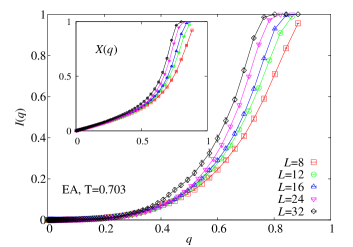
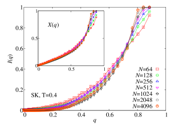
Figure 1: (Color online) Top: the median $I(q)$ of the cumulative overlap distribution as a function of $q$ for the $3D$ EAI model with temperature $T=0.703$. The inset shows the cumulative distribution $X(q)$ as a function of $q$. Bottom: the same curves for the SK model, with $T=0.4$.

The EAI model has not been simulated at exactly the same temperatures for the different lattice sizes we have studied (as opposed to the SK model where we have a consistent set of temperature values). Usually, the temperature dependencies are smooth and we can safely interpolate the data to the lowest temperature of the largest system ($T=0.703$). This procedure is followed in Fig. 1. For more complicated (and noisy) quantities, such as $f_{p}$, given the sensitivity to small errors, this procedure may be dangerous. Therefore, in the following we have only analyzed the larger system sizes, where the simulated temperatures where already very close to the value we have for $L=32$, $T=0.703$ ($T=0.697$ for $L=24$ and $T=0.698$ for $L=16$) and the possible error due to the temperature variation is negligible (see also Refs. Baños et al., 2011; Alvarez Baños et al., 2010a). In any case, as we shall see, even if the $q$-behavior of our studied quantities is $T$-dependent, we do not expect the $X$-behavior to be, so the precise temperature will not be relevant in the rest of the paper (we just need to ensure that we are as free as possible from critical effects, hence our choice of the lowest available temperatures).

If not specified otherwise, the error bars in the plots have been obtained with a bootstrap analysis Efron and Tibshirani (1994).

IV.2 Numerical results for the EAI and SK models

Let us start by considering $I(q)$ and $X(q)$ as a function of $q$, which we show for the EAI and the SK models in Fig. 1. In the SK model both $I(q)$ and $X(q)$ converge nicely to some limiting curve when $N$ increases. The major source of finite-size effects is apparently the well-known shift of $q_{\text{EA}}$ for increasing $N$ values Alvarez Baños et al. (2010a, b); Aspelmeier et al. (2008). The average $X(q)$ is linear in $q$ at the origin as expected. For small values of $q$ $I(q)$ is much smaller than $X(q)$, as expected from (8). The comparison with the plots of Ref. Middleton, 2013 for droplet-like models shows a marked difference, since there $I(q)$ is identically zero for small values of $q$. The study of the median of the distribution of $X_{J}(q)$ as a function of $q$ does distinguish clearly between droplet and RSB mean-field behavior. Trading the average for the median does make the analysis more clear cut.

The EAI data are very similar to those obtained from the SK model: both $I(q)$ and $X(q)$ for increasing values of $N$ nicely converge to some limiting curve (in agreement with the fact Alvarez Baños et al. (2010a) that $P(0)$ depends only very weakly on $L$). The limiting curve for $X(q)$ is linear at the origin. $I(q)$ is much smaller than $X(q)$ but it is definitely not identically equal to zero at low $q$, unlike in the droplet-like models of Ref. Middleton, 2013. In conclusion the study of the $q$ behavior of the median of the $X_{J}(q)$ distribution gives strong support to a RSB scenario for the 3D EAI model.

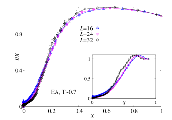
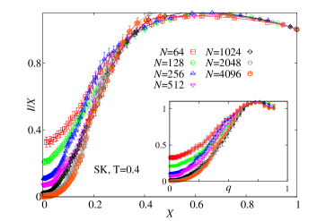
Figure 2: (Color online) The median to mean ratio $I(q)/X(q)$ as a function of $X(q)$ (main plots) and as a function of $q$ (insets). Top: 3D EAI data with $T\sim 0.7$; bottom: SK data with $T=0.4$. Note the much lager finite-size effects in the SK case.

In Fig. 2 we show the ratio $I/X$ as a function of $X$ (main plots) and of $q$ itself (insets) for both the EAI and SK models. The SK data show very strong finite-size effects as $q$ and $X$ go to zero. In contrast the EAI data show little finite-size effects. While this difference remains to be understood, the upshot is that in both the EAI and SK cases, the ratio $I/X$ is vanishing for small $X$ and for large system sizes, as expected from the RSB picture.

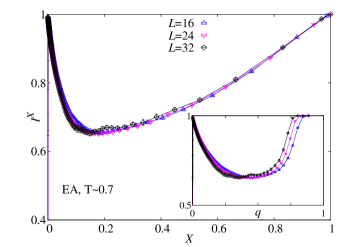
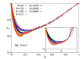
Figure 3: (Color online) $f(q)\equiv I(q)^{X(q)}$ as a function of $X(q)$ (main plots) and as a function of $q$ (insets). Top: $3D$ EAI model with $T\sim 0.7$. Bottom: SK model with $T=0.4$. Note the much larger finite-size effects in the SK case.

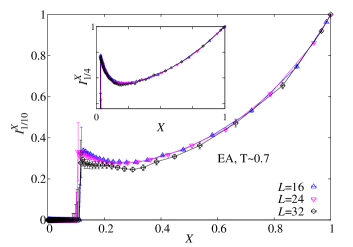
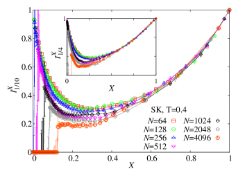
Figure 4: (Color online) The quantities $f_{1/10}$ (main plots) and $f_{1/4}$ (insets) as a function of $X$. Top: $3D$ EAI data with $T\sim 0.7$. Bottom: SK data with $T=0.4$.

In Fig. 3 we show $f(q)\equiv I(q)^{X(q)}$ as a function of $X(q)$ (main plots) and as a function of $q$ (insets) for both the EAI and the SK models. The interpretation of the SK data is clear: the data for increasing system sizes converge toward a smooth limiting curve, whose $q\to 0$ (or $X\to 0$) limit is compatible with the expected value $\frac{1}{2}$. The convergence fails when finite-size effects become important: for any given value of $N$ there is a crossover value $q^{*}=q$ below which $f$ enters a finite-size regime and goes to one as $q$ and $X(q)\to 0$. This $q^{*}$ goes to zero as $N\to\infty$. In other words, for each value of $N$ there is a value of $q$ below which the finite-size broadening of the peaks in the overlap distribution cannot be neglected, and the distribution of the $X_{J}$’s becomes a “nice distribution” whose median and average scale in the same way (possibly with different exponents) when $q\to 0$. We can summarize the situation by saying that $\lim_{q\to 0}\lim_{N\to_{\infty}}f=\frac{1}{2}$, but that at fixed, finite $N$ $\lim_{q\to 0}f=1$.

The overall situation is very similar for the EAI model (top part of Fig. 3). Here again we have a function decreasing, for decreasing $X$, down to a small value of $X$ and eventually increasing to one. Here the emergence of the thermodynamic behavior looks slower than for the SK model; this makes it difficult to estimate the infinite-volume limit of $f$ for $X\to 0$, but qualitatively it is crucial that we have the same kind of behavior than in the SK model, in the same range of $p$ values.

In Fig. 4 we show $f_{p}(X)$ for the lower-order quantiles $p=0.25$ and $p=0.1$ for both the EAI and SK models, that turn again, in both cases, to be consistent with RSB predictions. The data can be interpreted exactly like the $p=1/2$ data, with the difference that now the low $q$ data are severely affected by the finite $N_{q}$ bias presented above. All points where $I_{d}\ll 1/N_{q}$ are cut off, and $f_{p}=0$ in the whole region at the left of some size and quantile dependent threshold. As a collateral damage due to a statistical bias (and not to a physical effect) the finite-size rise of $f_{p}$ towards $1$ as $q\to 0$ (or $X\to 0$) is lost. Again in the EAI model we observe a far weaker volume dependence than in the SK model, and we only detect slow and weak hints of the emergence of the thermodynamical behavior of the system.

IV.3 Comparison of the numerical results with the mean-field expectations

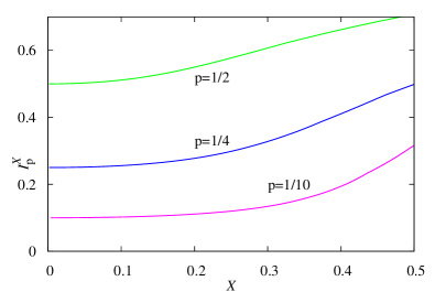
Figure 5: (Color online) Prediction for $f_{p}=I_{p}(q)^{X(q)}$ as a function of $X(q)$ using the self-consistent approximation of Eq. 11. Curves are drawn for $p=\frac{1}{2}$ (i.e., for the median), for $p=\frac{1}{4}$ and for $p=\frac{1}{10}$.

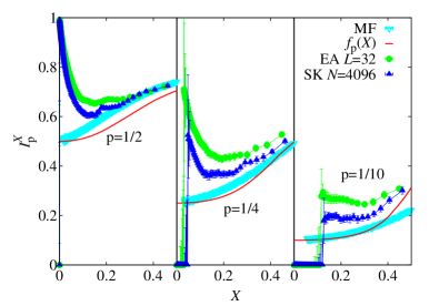
Figure 6: (Color online) We compare the self-consistent approximation of Eq. 11, $f_{p}(X)$, to the data obtained for the largest lattice sizes both for the EAI and the SK models. We also include the mean-field prediction, as constructed from a weight-generation method (see text and Marinari et al. (1998)). We show on the left $p=\frac{1}{2}$ (i.e., the median), in the center $p=\frac{1}{4}$ and on the right $p=\frac{1}{10}$.

In this subsection, we compute the function $f_{p}(q)$ in the mean-field theory beyond the simplest approximation used in the previous subsection (namely $f_{p}(X)=p$). We consider two different approximate methods, and compare the results to our numerical data. As we have discussed before, the prediction of Eq. (7) only holds as $q\to 0$ (and it is not even self-consistent). As a modest improvement we can make it self-consistent while keeping the correct $q\to 0$ behavior, writing $\mathbb{P}(s)=A(X)s^{X-1}+B(X)$, where $A(X)$ and $B(X)$ are fixed by the normalization of $\mathbb{P}(s)$ and by self-consistency (the relation analogous to Eq. (10)). For instance, when $B(X)=0$ then $A(X)=X$ and $f_{p}=p$. This can be done at least when $X<0.5$, with the result:

$$\mathbb{P}_{C}(s)=\frac{s}{1-X}\left\{s^{X-1}\left(1-X-2X^{2}\right)+2X^{2}\right\}\;.$$ (11)

Now computing $\mathbb{P}_{c}(s)$ at $s=I_{p}$ gives, for $f_{p}\equiv I_{p}^{X}$, the equation

$$\frac{1}{1-X}\left(\left(1-X-2X^{2}\right)f_{p}+2X^{2}f_{p}^{\frac{1}{X}}\right)=p\;.$$ (12)

We show in Fig. 5 the functions $f_{p}(X)$ as obtained by this simple modification of Eq. (8): one has, as expected, $\lim_{X\rightarrow 0}f_{p}=p$, and $f_{p}$ is a monotonic function of $X$ which is almost flat near $X=0$.

There is an alternative approach to the estimation of $f_{p}$. Indeed, the function $\mathbb{P}(s=X_{J})$ is actually known in mean field for a given value of $X$ (see Mézard et al. (1987, 1985)). The full equations are complicated, but there is a simple numerical method Marinari et al. (1998) that can be used to sketch the behavior of $I_{p}(X)$. Essentially, we take advantage of the ultrametric structure of the spin-glass phase to group the states in clusters at any value of $X$. We consider a system where $M$ such clusters are allowed, each with a weight $w_{a}=C\exp(-f_{a})$, where $C$ is such that $\sum_{a}w_{a}=1$. The $f_{a}$ are i.i.d random variables distributed according to $p(f_{a})=B\exp(Xf_{a})$. We can then use this set of weights to compute the $X_{J}$ for a given sample. This method provides no relation between the $X_{J}$ for a fixed sample at different levels of $X$, so it cannot be used to generate the full $P_{J}(q)$, but it is useful to sketch the behavior of $I_{p}(X)$ and, hence, of $f_{p}$ (at least for not too small values of $X$: for $X\ll 1$ the method involves the sampling of huge or tiny numbers and the numerical computation breaks down) .

In Fig. 6 we show the predictions of the self-consistent approximation together with the weight-generation method and with the numerical data for the largest lattice size for both our models. The qualitative agreement is very reasonable, specially for the small-$X$, small-$p$ sector.

V THE DROPLET PICTURE AND THE TOY MODELS

Thus far we have described the expected scaling behavior of the cumulative overlap distribution in the RSB picture, and we have checked that our numerical data are compatible with it, both for the SK and for the EAI model. The next step would be to make the analogous test comparing to the expected scaling behavior in the droplet theory. However, in this picture, a specific prediction for the finite-size behavior of these quantities is not available. Therefore, in order to test the hypothesis of a droplet-like behavior of the EAI model, we introduce several droplet-like (single-state) toy models, and we will compare their behavior with the one emerging from our numerical data. In addition, we introduce several many-state toy models (representing a simplified mean-field picture), in order to discuss to which extent the validity of (7) is an unavoidable consequence of the existence of a non-trivial overlap distribution.

V.1 Definitions of toy models

• Models $D2$ and $D3$. First, we consider a version of the toy model of Ref. Hatano and Gubernatis, 2002, described and studied in Ref. Middleton, 2013. For a system of size $L$, one defines a sample as a set of independent active droplets. These are group of spins that always keep their relative orientations but may flip as a whole, with probability $\frac{1}{2}$. These droplets are, in this model, quenched in size, and their distribution embeds the quenched disorder that characterizes the model: each droplet has a fixed, defined size, that does not change in time. On such a droplet sample one studies thermal averages where droplet signs change, as we said, with probability one half, allowing us to compute, among others, the overlaps in a given sample. The number $n_{v}$ of active droplets of size $v$ is Poisson distributed, with mean $n_{v}=c\,v^{-x}L^{D}$, where $x=2+\theta/D$, so that the average number of droplets of size $\ell^{D}$ scales as $\ell^{-D-\theta}$, as expected in the droplet scenario. In this toy model droplets are not defined relative to a lattice, and the dimension $D$ is just a parameter. We proceed in two phases. We first fix a sample by defining the droplets, and second we dynamically change their sign, computing in this way expectation values for a given sample. We generate a sample by extracting numbers of droplets with size up to $L^{D}/2$ from the Poisson distribution (for very small $L$ values it can happen that $\sum_{v=1}^{L^{D}/2}vn_{v}>L^{D}$: in this case we discard the sample and try again) and we add to it an extra (large) droplet of size $L^{D}-\sum_{v}vn_{v}$. Following Ref. Middleton, 2013, we consider two versions of the model: the model D$2$, where $D=2$, $\theta=0.5$ and $c=0.1$ (mimicking a two-dimensional droplet system), and the model D$3$, where $D=3$, $\theta=0.21$ and $c=0.0375$ (for a three-dimensional version of the model). With this choice of parameters in the $D=2$ model the “large” droplet occupies in average close to $54\%$ of the lattice, while in the $D=3$ case it takes close to $44\%$ of the lattice.

• Model $PK0$. Here we define the model by assigning the overlap probability distribution $P_{J}(q)$. We take for $P_{J}(q)$ a pair of Gaussian distributions with fixed width $\sigma$ centered at random positions $\pm q_{J}$:

  $$P_{J}(q)=\frac{1}{\sqrt{8\pi\sigma^{2}}}\left\{e^{-\frac{(q+q_{J})^{2}}{2\sigma^{2}}}+e^{-\frac{(q-q_{J})^{2}}{2\sigma^{2}}}\right\}\;,$$ (13)

  By varying $\sigma$ we can mimic the broadening of the distribution due to finite-size effects. The value of the peak locations is extracted from a hard-tail probability density:

  $$\begin{split}\mathcal{F}(q_{J};\epsilon)&\propto\epsilon^{-1}\exp{\left(-\frac{1}{1-\left((q_{J}-q_{J_{0}})/\epsilon\right)^{2}}\right)}\;,\\ \mathcal{F}(q_{J};\epsilon)&=0\ \mbox{when}\ \left|q_{J}-q_{J_{0}}\right|\geq\epsilon\end{split}$$ (14)

  which behaves like a delta function $\delta(q_{J}-q_{J_{0}})$ in the $\epsilon\rightarrow 0$ limit. In this over-simplified description, the two-state picture corresponds to the $\epsilon\to 0$ limit of the model. In the following we will take $q_{J_{0}}=0.7$.

• Model $PK\lambda$. In a slightly more elaborated version of PK0, we allow for more peaks, besides the one at $q_{J_{0}}$, to contribute to $P_{J}(q)$ for $q_{J_{0}}\geq q\geq 0$. Here a sample has a random number $N_{J}$ of secondary peaks at locations $q_{k}$, with $k=0,\dots,N_{J}-1$. The number of secondary peaks $N_{J}$ is a Poisson-distributed random variable with mean $\lambda$. The secondary peaks locations are uniformly distributed in the interval $[0,q_{J_{0}}]$, and the weights of the primary peak $W_{N_{J}}$ and of each of the $N_{J}$ secondary peaks $W_{k}$ are i.i.d. with uniform probability density. $P_{J}(q)$ is then a sum of pairs of Gaussian distributions:

  $$\begin{split}P_{J}(q)=\sum_{k=0}^{N_{J}}\frac{W_{k}}{\sqrt{8\pi\sigma^{2}}}&\left\{e^{-(q+q_{k})^{2}/2\sigma^{2}}\right.\\ &+\left.e^{-(q-q_{k})^{2}/2\sigma^{2}}\right\}\;.\end{split}$$ (15)

  where $q_{N_{J}}=q_{J_{0}}$. Also here we take $q_{J_{0}}=0.7$. This model can be seen as a many-states version of the PK$0$ model proposed above. For a given disorder realization the quenched disorder is given by the positions of the peaks and their weights, i.e.,

  $$\left\{J\right\}=\left\{q_{J},W_{N_{J}},q_{k=0,\dots,N_{J}-1},W_{k=0,\dots,N_{J}-1}\right\}\;.$$

  $X_{J}(q)$ can be easily computed as a sum of error functions.

• Model $UB\lambda$. Our last toy model uses a random branching process Parisi (1993) to construct hierarchical trees of states. Starting from the root node at $X=0$, and incrementing $X$ in small steps $\delta X$ up to $X_{M}$, we allow any branch to bifurcate randomly at each step with a given fixed probability $\frac{\lambda\;\delta X}{X_{M}}$, such that any path from the root to any leaf has an average number of bifurcations equal to $\lambda$. At a bifurcation, the weight of each new branch is assigned extracting two free energy values $F_{1}$ and $F_{2}$ and constraining the two weights $w_{i}\propto\exp(-F_{i})$ to sum up to the weight of the ancestor, as described in Refs. Mézard et al., 1985; Parisi, 1993. In order to map $X$ values to $q$ values, we simply take $X(q)$ to be a linear function of $q\in[0,q_{J}]$ with $q_{J}$ extracted as in the PK$\lambda$ toy model. At each level of $X$, $X_{J}(q)=1-\sum w_{i}^{2}$, where the sum extends to all branches that have already spawned. As $X_{J}(q)$ is a piece-wise constant function, the overlap probability density of the single sample is a sum of delta functions, that we smooth by Gaussian convolutions exactly as in the PK$\lambda$ toy model. It would take an infinite branching process and a precise knowledge of the function $X(q)$ to accurately reproduce the results from the mean-field theory Parisi et al. (2014). Still this toy model has, by construction, interesting properties such as ultrametricity, non-self-averageness and a non-trivial average $P(q)$. In our computation we set $X_{M}=X(q_{J})=0.5$ and $q_{J_{0}}=0.7$. For $\lambda=0$ the two toy models UB$0$ and PK$0$ coincide.

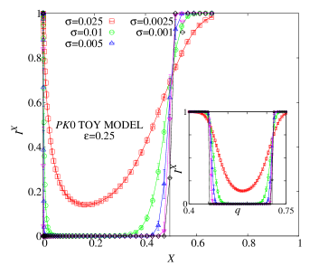
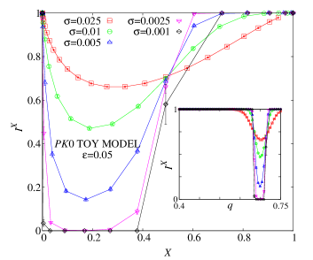
Figure 7: (Color online) PK$0$ toy model: $f\equiv I(q)^{X}(q)$ as a function of $X(q)$ (main plots) and as a function of $q$ (insets). $q_{J_{0}}=0.7$. Top: the width of the distribution of the position of the peak is $\epsilon=0.25$. Bottom: $\epsilon=0.05$.

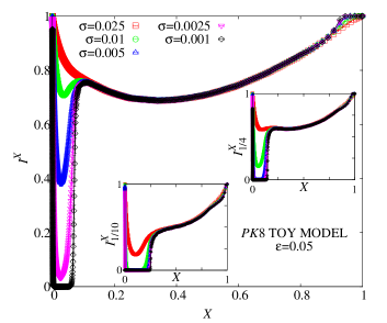
Figure 8: (Color online) PK$8$ toy model: $f_{p}$ as a function of $X$, for $p=1/2$ (main plot), $p={1/4}$ and $p={1/10}$ (insets).

V.2 Numerical results for the toy models

Using these toy models we can check whether the results obtained in Sec. IV are really a consequence of the existence of a RSB-like spin-glass phase or just a numerical artifact.

The PK$0$ model reproduces, by tuning the $\epsilon$ and $\sigma$ parameters, the trivial distribution one expects for a large system in a droplet-like picture. When the distribution of the self-averaging peak’s position $q_{J}$ is a narrow delta ($\epsilon\rightarrow 0$) around $q_{J_{0}}$, the $X_{J}(q)$ of most samples are all very close, since their values depend almost exclusively on $\sigma$. At intermediate overlap values $q\sim q_{J_{0}}-\epsilon$, the few samples for which $q_{J}\lesssim q$ dominate the mean value, while the median (or any other smaller quantile) stays small, and $f_{p}$ is depressed. Outside such region, $I_{p}$ and $X$ are either both very small (low $q$) or both of order one ($q\gtrsim q_{J_{0}}$), that implies $f_{p}\sim 1$. As one can see from the insets in Fig. 7, the region in which $f_{p}$, when seen as a function of $q$, is significantly different from unity shrinks when $\epsilon$ decreases. Since, by construction, we cannot have samples with $q_{J}<q_{J_{0}}-\epsilon$, for any (not too large) $\epsilon$ values all $X_{J}(q)$ are vanishing at small but non-zero $q$ values when $\sigma\to 0$. As a function of $X$, $f_{p}$ is almost one above $X(q_{J_{0}}+\epsilon)$, and almost zero below $X(q_{J_{0}}-\epsilon)$. As a function of $q$, we have a dip that gets sharper and deeper as $\sigma$ decreases. The dip width shrinks as $\epsilon$ gets smaller, and the values of $X$ cluster in two narrowing regions around $X=0$ and $X=1$ respectively. In PK$0$ then, at large $\sigma$, $f$ is zero at small $X$ but it is one at $X\sim 0$, or, in terms of the overlap, $f$ is zero in an interval of size $\sim\epsilon$ around $q_{J_{0}}$ and it is one everywhere else.

The PK$\lambda$ toy model adds a non-self-averaging contribution to the overlap distribution. The secondary peaks can be centered at any values of $q\lesssim q_{J}$, down to $q\sim 0$. When the distribution of the self-averaging peak position $q_{J}$ gets narrower (i.e., when $\epsilon$ gets smaller), a strong depression in the median (and in the lower quantiles) is still possible at low $q$ and at small $\sigma$, because the median of the position of the leftmost peak (the median of the smallest $q_{k}$ value) has a finite distance from $q=0$. As the number of allowed peaks grows, the dip does eventually shrink to $q\sim 0$, but for large values of $\lambda$ the model becomes trivial since it loses non-self-averageness. We show in Fig. 8 an example of what happens in the PK$8$ model (where $\lambda=8$, i.e., there are in average eight secondary peaks). The dip at low $X$ values is due to the fact that at low $q$ values there are no peaks. When the number of peaks increases one gets more peaks close to to $q=0$ and gets additional contributions to $f_{p}$, which can become different from zero down to very low $X$ values. Apart from the dip, which is built-in in the toy model but is related to finite-statistics artifacts in the spin-glass models (and disappears for these models in the limit of an infinite number of samples), PK$8$ has a qualitative similarity with the EAI and the SK model. We computed averages and quantiles for PK$0$ and PK$8$ from $10000$ different disorder samples.

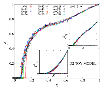
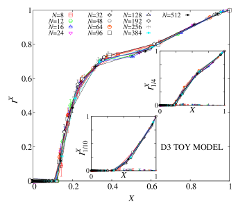
Figure 9: (Color online) Droplet-like toy models: $f_{p}$ as a function of $X$, $p=1/2$ (main plots), $p={1/4}$ and $p={1/10}$ (insets). Top: D$2$ toy model. Bottom: D$3$.

We find a completely different behavior in the D$2$ and D$3$ models (see Fig. 9). In this case we computed overlaps by randomly flipping clusters: to minimize the effects of a limited number of measurements, we preferred to simulate a reasonable but not huge number of samples ($1000$) and to collect a fairly large number of measurements per sample for the largest sizes ($10^{10}$ for $L\geq 64$ in D$2$ and $10^{8}$ for $L\geq 16$ in D$3$). Although this model has been used in Ref. Middleton, 2013 to provide an example of finite-size effects persisting up to very large system sizes, the almost perfect collapse of data for all simulated sizes, when plotted as a function of $X$, is striking. The quantities $f_{p}$ are rapidly decreasing with $X$, and are almost zero in a wide interval down to $X=0$. The possibility of finite-statistics effects driving the sudden drop in $f$ cannot be completely ruled out.

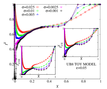
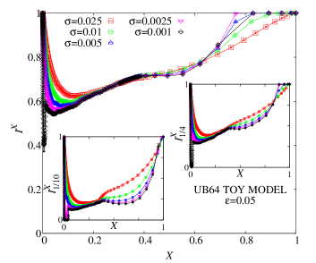
Figure 10: (Color on-line) Random bifurcation toy model: $f_{p}$ as a function of X, $p=1/2$ (main plots), $p={1/4}$ and $p={1/10}$ (insets). Top: UB$8$; bottom: UB$64$.

Finally, in Fig. 10, we show $f_{p}$ for $p=1/2$, $1/4$, $1/10$, for the UB$\lambda$ toy model. We have averaged over $10000$ instances of the quenched noise. The data for high branching probability closely resemble those of the SK model, also for the dependence on the system size (we mimic finite-size effects by tuning $\sigma$). Since a finite fraction of samples have no weight at low $X$, a narrow dip is present near $X=0$ for small $\sigma$ value. As the forking probability grows, so does the fraction of samples with peaks in the $P_{J}(q)$ at small $q$ values, and the dip shrinks away. The curves for larger values of $\sigma$ show the steep rise towards the $f(X=0)=1$ singularity, as in the case of our data for the spin-glass models. At small $\sigma$ and large $\lambda$ the curves have the expected limit $f_{p}(X{\rightarrow 0})=p$. Unfortunately, the spin-glass data do not allow a fair extrapolation of a possible size-dependent $f_{p}(0)$ limit to compare with.

The conclusion of this exercise based on toy models is that in order to produce a behavior of $f_{p}$ similar to the one observed for the SK and 3D EAI models, one needs many states. In particular, the droplet toy model completely fails to reproduce the observed qualitative behavior.

VI CONCLUSIONS

The question of the large-volume extrapolation of numerical data for the overlap distribution of spin-glass models has been a subject of controversy over the years. Recently, Ref. Middleton, 2013 has proposed the use of $I(q)$, the median over disorder samples of the overlap cumulative distribution, showing that for some droplet-like models it converges rapidly to zero in a whole interval of overlap values close to the origin. This is very different, and more clarifying, than the slow convergence of the mean $X(q)$. We use $I(q)$ (and its generalization to different quantiles) to study the SK and the $3D$ EAI models. The results of the two models are very similar and unmistakably different from the one that is obtained for the droplet-like models of Ref. Middleton, 2013, making the case for a RSB-like behavior of the $3D$ EAI model in the spin-glass phase.

We have studied $I_{p}(q)$, the quantiles over disorder samples of the overlap cumulative distribution, comparing our numerical estimates of $f_{p}(q)=I_{p}(q)^{X(q)}$ with the predictions of the RSB theory for the SK model. The numerical results for the SK model converge (although non-uniformly) as $N$ grows towards the RSB predictions for the low $X(q)$ behavior of $f_{p}(q)$. The results for the EAI model are again qualitatively very similar to the one obtained in the mean field theory, even if the infinite-volume limit seems clearly more difficult to reach in the finite dimensional theory.

We have also studied several toy models, which show that the observed behavior of $f_{p}$ is connected to the existence of many thermodynamic states.