Abstract

We propose an approach to generate geometric theorems from electronic images of diagrams automatically. The approach makes use of techniques of Hough transform to recognize geometric objects and their labels and of numeric verification to mine basic geometric relations. Candidate propositions are generated from the retrieved information by using six strategies and geometric theorems are obtained from the candidates via algebraic computation. Experiments with a preliminary implementation illustrate the effectiveness and efficiency of the proposed approach for generating nontrivial theorems from images of diagrams. This work demonstrates the feasibility of automated discovery of profound geometric knowledge from simple image data and has potential applications in geometric knowledge management and education.

1 Introduction

Diagrams have been used to illustrate geometric theorems and problems for thousands of years and can be produced now by using computer programs with ease. A number of software tools developed in the area of dynamic geometry are capable of generating dynamic diagrams automatically from specifications of geometric theorems [33]. This paper tackles the inverse problem: given the electronic image of a diagram, generate the specifications of one or more theorems which the diagram may be used to illustrate. An ideal solution to this problem allows one to generate geometric theorems automatically from their illustrations available in electronic documents and resources.

To be specific, let us restrict our study to plane Euclidean geometry in this paper. The approach we propose to solve the above-stated problem consists of the following main steps.

1. Retrieve geometric information, mainly geometric objects and their labels, in the given image of diagram using techniques of pattern recognition (in particular Hough transform as discussed in Sections 2.1 and 2.2).

2. Mine geometric relations among the retrieved geometric objects from predetermined potential relations by examining their corresponding algebraic relations using numeric verification (see Section 2.3).

3. Generate candidate propositions from the mined geometric relations by using six strategies introduced (see Section 3.1).

4. Obtain theorems from the generated candidate propositions using algebraic methods, first to rule out false propositions efficiently by checking numeric instances and then to prove the true propositions via symbolic computation (see Sections 3.2 and 3.3).

These four steps are described in detail in the following two sections. We have implemented the proposed approach. Preliminary experiments with our implementation are reported in Section 4. Some related work on geometric information retrieval and theorem discovery is discussed briefly in Section 5. The paper concludes with a few remarks in Section 6.

The work presented in this paper demonstrates for the first time the feasibility of discovering rigorous and profound geometric knowledge (theorems) from inexact and partial geometric data (images of diagrams) automatically. This feasibility brings us the hope to build up a large-scale database of geometric theorems automatically or semi-automatically by searching diagrams from electronic documents and resources accessible via the Internet. Theorems collected in such a database will have standardized formal representations and are linked to images of diagrams. The processing and management of theorems in the database, including searching, organization, translation (into representations in natural languages or algebraic expressions), and degenerate-case handling, would be made easier or more efficient.

A potential application of our work in education is evident. An extension of the proposed approach to dealing with hand-drawn diagrams could make it possible for students to submit geometric theorems to provers by simply sketching their diagrams on mobile computing devices.

2 Information Retrieval from Images of Diagrams

Geometric information consists of geometric objects (i.e., shapes used in geometric diagrams), their labels (i.e., identifiers of the objects), and geometric relations (i.e., properties and features of the objects). In what follows, we discuss how to retrieve information from images of diagrams and how to represent it in a processable form for theorem generation.

2.1 Recognizing Basic Geometric Objects

In our current investigation we consider the following three types of basic geometric objects which are used to form most of the diagrams in plane Euclidean geometry.

• Points. A point is represented by a pair of coordinates $(x,y)$ in the coordinate system determined by the image of diagram, where the parameters $x$ and $y$ are called $x$-coordinate and $y$-coordinate, respectively.

• Lines. A straight line (with no extremes) is represented by line$(P_{1},P_{2})$, where the parameters $P_{1}$ and $P_{2}$ denote two distinct points incident to the line. Similarly, a half line is represented by halfline$(O,P)$, where the parameter $O$ denotes its initial point and $P$ denotes a point on it; a segment is represented by segment$(E_{1},E_{2})$, where the parameters $E_{1}$ and $E_{2}$ denote the endpoints of the segment. For the sake of convenience, all straight lines, half lines, and segments, with respective types line, halfline, and segment, are called lines.

• Circles. A circle may be represented by circle$(O,r)$, where the parameter $O$ denotes the center of the circle and $r\leavevmode\nobreak\ (>0)$ denotes the radius of the circle, and by circle$(A,B,C)$, where the parameters $A$, $B$, and $C$ denote three distinct points on the circle.

A geometric object may be referred to by an identifier which is called the label of the object. For example, the point $(x,y)$ with label $P$ is represented as $P:=(x,y)$; the straight line with label $l$ passing through $P_{1}$ and $P_{2}$ is represented as $l:=\mbox{{line}}(P_{1},P_{2})$.

Recognition of a basic geometric object $\mathcal{O}$ means to determine the parameter values of $\mathcal{O}$. For example, a circle can be recognized by determining the coordinates of its center and the value of its radius.

Our approach to recognizing basic geometric objects from images of diagrams is based on Hough transform [10], a general technique for estimating the parameters of a shape from its boundary points. Through Hough transform, the detection of a shape is converted to a voting procedure carried out in a parameter space. For instance, the detection of a line can be realized by checking whether the number of curves (corresponding to the points on the line) crossing at a certain point (corresponding to the line) in the parameter space is greater than a threshold. However, due to the effects of image quality, line width, and concrete recognition requirements, the results obtained via Hough transform might not perfectly reflect the actual features of the geometric diagrams. For example, a line may be detected as several disconnected short segments; the position and the size of a circle may be not the same as they are in the diagram. To improve the accuracy of recognition for basic geometric objects, we adopt some techniques to refine the results of Hough transform, as described in the following algorithm.

Algorithm 1 (Geometric object recognition).

Given an image $\mathrm{I}$ of diagram, output a set $\mathbb{C}$ of circles, a set $\mathbb{L}$ of lines, and a set $\mathbb{P}$ of points of interest contained in $\mathrm{I}$.

Step 1.1.

[Recognize circles]

1.1.1.

[Preprocess] Perform graying and smoothing operations on the image $\mathrm{I}$ (using, e.g., the technique of Gaussian smoothing given in [30]) to obtain a new image $\mathrm{I}_{1}$.

1.1.2.

[Detect] Apply the gradient-based Hough transform (see algorithm 21HT in [27]) on $\mathrm{I}_{1}$ to acquire a set $\mathbb{C}$ of circles.

1.1.3.

[Refine] For each $c:=\mbox{{circle}}(O,r)$ in $\mathbb{C}$, collect four points $P_{1}$, $P_{2}$, $P_{3}$, and $P_{4}$ on the left-bound, right-bound, top-bound, and bottom-bound of $c$ respectively, and then replace $O$ by the centroid of the quadrilateral $P_{1}P_{2}P_{3}P_{4}$ and $r$ by the average of the Euclidean distances $\|OP_{1}\|$, $\|OP_{2}\|$, $\|OP_{3}\|$, and $\|OP_{4}\|$.

Step 1.2.

[Recognize lines] There are three possible defects in the lines detected from an image of diagram by applying Hough transform: (1) a line in the diagram is detected as some disconnected short segments; (2) the endpoints of a segment cannot be accurately detected; (3) some nonexisting segments may be detected on a circle, in particular when the radius of the circle is large. The following substeps are used to amend the defects.

Step 1.3.

[Collect points of interest] The set $\mathbb{P}$ of points of interest are obtained as follows.

• For each $\mbox{{circle}}(O,r)$ in $\mathbb{C}$, add $O$ to $\mathbb{P}$; for each $\mbox{{circle}}(A,B,C)$ in $\mathbb{C}$, add $A$, $B$, and $C$ to $\mathbb{P}$.

• For each $\mbox{{line}}(P,Q)$, or $\mbox{{halfline}}(P,Q)$, or $\mbox{{segment}}(P,Q)$ in $\mathbb{L}$, add $P$ and $Q$ to $\mathbb{P}$.

• For each pair of lines in $\mathbb{L}$, compute the numeric coordinates of the intersection point $P$ of the two lines and add $P$ to $\mathbb{P}$, if $P$ exists.

• For each pair of a line in $\mathbb{L}$ and a circle in $\mathbb{C}$, compute the numeric coordinates of the intersection points $P_{1}$ and $P_{2}$ of the line and the circle and add $P_{1}$ and $P_{2}$ to $\mathbb{P}$, if $P_{1}$ and $P_{2}$ exist.

• For each pair of circles in $\mathbb{C}$, compute the numeric coordinates of the intersection points $P_{1}$ and $P_{2}$ of the two circles and add $P_{1}$ and $P_{2}$ to $\mathbb{P}$, if $P_{1}$ and $P_{2}$ exist.

Due to errors of numeric computation, the same point in the diagram may be collected into $\mathbb{P}$ more than once with different coordinates. Therefore, in the above process of adding a point $P$ to $\mathbb{P}$, the following substep need be performed to check whether $P$ is already contained in $\mathbb{P}$.

To each of the recognized basic geometric objects, it is necessary to assign a unique label (or letter), so that geometric relations among the objects can be expressed clearly. Labels for important geometric objects (such as points) are usually contained in diagrams. We shall present a method to extract information on label assignment from images of diagrams in the next subsection.

2.2 Recognizing Labels of Geometric Objects

Labels in an image of diagram may be recognized by checking whether each of them matches a character template, as shown in the following algorithm.

Algorithm 2 (Label recognition).

Given an image $\mathrm{I}$ of diagram and the three sets $\mathbb{C}$, $\mathbb{L}$, and $\mathbb{P}$ obtained by applying Algorithm 1 to $\mathrm{I}$, output a list $\mathbf{L}$ of labels in $\mathrm{I}$ and a list $\mathbf{P}$ of the corresponding centers of the regions where the labels occur in $\mathrm{I}$.

To assign the recognized labels to corresponding geometric objects, we adopt the following strategies according to the convention that in geometry, usually a letter in upper case is used to label its nearest point and a letter in lower case is used to label its nearest line. For the $i$th label $L_{i}$ in $\mathbf{L}$, if $L_{i}$ is in upper case, then it is assigned to a point $P$ in $\mathbb{P}$ such that for any other point $P^{\prime}\in\mathbb{P}$, $\|C_{i}P\|<\|C_{i}P^{\prime}\|$, where $C_{i}$ is the $i$th point in $\mathbf{P}$; if $L_{i}$ is in lower case, then it is assigned to a line $l$ in $\mathbb{L}$ such that for any other line $l^{\prime}\in\mathbb{L}$, $\|C_{i}l\|<\|C_{i}l^{\prime}\|$.

For any geometric object that is not labeled in the image, a unique label is automatically generated by our program to refer to the object. Taking the image of a diagram (Fig. 1) for Simson’s theorem as an example, we show the geometric objects obtained by Algorithm 1 and the labels recognized by Algorithm 2 or generated automatically.

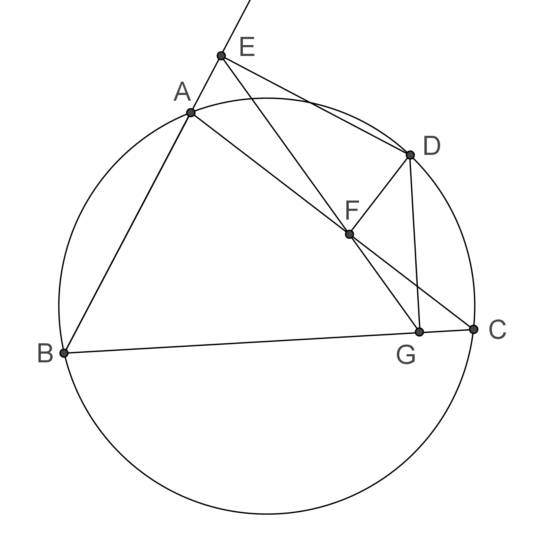
Figure 1: An image of diagram for Simson’s Theorem

• The set $\mathbb{P}$ of points of interest:

  $$\begin{array}[]{llll}\vskip 3.0pt plus 1.0pt minus 1.0ptB:=(45,260),&C:=(351,243),&G:=(313,246),&A:=(137,78),\\ \vskip 3.0pt plus 1.0pt minus 1.0ptF:=(262,174),&H:=(311,212),&E:=(163,37),&I:=(182,0),\\ D:=(305,110),&J:=(196,224),&K:=(184,67),&L:=(224,69).\end{array}$$

• The set $\mathbb{L}$ of lines:

  $$\begin{array}[]{lll}\vskip 3.0pt plus 1.0pt minus 1.0pta:=\mbox{{segment}}(B,C),&b:=\mbox{{segment}}(A,C),&c:=\mbox{{segment}}(E,G),\\ \vskip 3.0pt plus 1.0pt minus 1.0ptd:=\mbox{{halfline}}(B,I),&e:=\mbox{{segment}}(E,D),&f:=\mbox{{segment}}(D,G),\\ g:=\mbox{{segment}}(F,D).\end{array}$$

• The set $\mathbb{C}$ of circle: $h:=\mbox{{circle}}(J,157)$.

The features of diagrams are depicted mainly via geometric relations (e.g., incidence, perpendicularity, and parallelism) among the involved objects. Geometric relations play a fundamental role in the specification of geometric knowledge (e.g., theorems). Based on retrieved information about geometric objects, we shall present a method to mine geometric relations in the next subsection.

2.3 Mining Basic Geometric Relations

Some geometric relations such as those listed in Table 1 may be taken as basic geometric relations because they can be used to describe most features about the size and position of geometric objects and from them many other geometric relations can be derived. For example, if point $A$ is incident to line $p$ and also to line $q$, then the two relations derive the new relation that $A$ is the intersection point of the two lines $p$ and $q$.

Table 1: Basic geometric relations

Type	Representation	Meaning
onLine	$\mbox{{incident}}(A,\!l)$	point $A$ lies on straight line $l$, or segment $l$, or half line $l$
onCircle	$\mbox{{pointOnC}}(A,\!o)$	point $A$ is on circle $o$
Parallel	$\mbox{{parallel}}(l_{1},\!l_{2})$	$l_{1}$ is parallel to $l_{2}$
Perp	$\mbox{{perpendicular}}(l_{1},\!l_{2})$	$l_{1}$ is perpendicular to $l_{2}$
dEqual	$\mbox{{equal}}(\mbox{{distance}}(A,\!B),\mbox{{distance}}(C,\!D))$                      or $\|AB\|\!=\!\|CD\|$	the Euclidean distance between $A$ and $B$ is equal to that between $C$ and $D$
aEqual	$\mbox{{equal}}(\mbox{{size}}(\mbox{{angle}}(A,\!B,\!C)),\!\mbox{{size}}(\mbox{{angle}}(D,\!E,\!F)))$ or $\angle ABC\!=\!\angle DEF$	the size of $\angle ABC$ is equal to the size of $\angle DEF$

Each basic geometric relation in Table 1 corresponds to an algebraic equality in the coordinates of the involved points and the radii of the involved circles. In general, a geometric relation can be certificated to be true if and only if its corresponding equality holds. Take $\mbox{{incident}}(C,\mbox{{line}}(A,B))$ as an example and let the coordinates of $A$, $B$, and $C$ be $(x_{1},y_{1})$, $(x_{2},y_{2})$, and $(x_{3},y_{3})$, respectively. To determine whether $C$ lies on line $AB$, one can check whether the value of the expression $x_{1}y_{2}+x_{2}y_{3}+x_{3}y_{1}-x_{1}y_{3}-x_{2}y_{1}-x_{3}y_{2}$ is equal to $0$. However, due to recognition and numeric errors, it is not effective to determine the equality by simply evaluating the expression, in particular when the slope of the line is large. We adopt some techniques to mine basic geometric relations as detailed in the following algorithm.

Algorithm 3 (Geometric relation mining).

Given the set $\mathbb{P}$ of points of interest, the set $\mathbb{L}$ of lines, and the set $\mathbb{C}$ of circles recognized from an image of diagram with labels, output a set $\mathbb{R}$ of basic relations among the geometric objects.

Using Algorithm 3, one may obtain the following basic geometric relations for Fig. 1:

$$\begin{array}[]{l}\vskip 3.0pt plus 1.0pt minus 1.0pt\mbox{{incident}}(G,a),\leavevmode\nobreak\ \mbox{{incident}}(A,d),\leavevmode\nobreak\ \mbox{{incident}}(F,b),\leavevmode\nobreak\ \mbox{{incident}}(F,c),\\ \vskip 3.0pt plus 1.0pt minus 1.0pt\mbox{{incident}}(H,f),\leavevmode\nobreak\ \mbox{{incident}}(E,d),\leavevmode\nobreak\ \mbox{{incident}}(K,c),\leavevmode\nobreak\ \mbox{{incident}}(L,e),\\ \vskip 3.0pt plus 1.0pt minus 1.0pt\mbox{{incident}}(H,b),\leavevmode\nobreak\ \mbox{{pointOnC}}(B,h),\leavevmode\nobreak\ \mbox{{pointOnC}}(C,h),\leavevmode\nobreak\ \mbox{{pointOnC}}(A,h),\\ \vskip 3.0pt plus 1.0pt minus 1.0pt\mbox{{pointOnC}}(K,h),\leavevmode\nobreak\ \mbox{{pointOnC}}(L,h),\leavevmode\nobreak\ \mbox{{pointOnC}}(D,h),\\ \mbox{{perpendicular}}(a,f),\leavevmode\nobreak\ \mbox{{perpendicular}}(b,g),\leavevmode\nobreak\ \mbox{{perpendicular}}(d,e).\end{array}$$

3 Automated Generation of Geometric Theorems

It is remarkable that geometric objects and their relations retrieved from a single image of diagram allow certain nontrivial properties implied in the diagram to be expressed explicitly. Such properties often hold generally for families of diagrams and may be stated as propositions. A geometric theorem is a true proposition about the implication of a geometric relation (called the conclusion of the theorem) in all the diagrams that satisfy the same set of geometric relations (called the hypothesis of the theorem). It is surprising that geometric theorems can be generated automatically and effectively from the information retrieved from images of diagrams in three steps: generating candidate propositions, ruling out false candidates, and proving the obtained theorems.

3.1 Generating Candidates

A candidate proposition is one that is likely a theorem. It can be generated in a simple way by selecting one (or more) geometric relation(s) as the conclusion and taking some other relations as the hypothesis. As there are geometric objects and relations which are irrelevant to the features of the diagram, it is necessary to remove such objects and relations for the efficiency of theorem mining from candidate propositions.

Usually more points of interest than needed are recognized from the diagram. A point of interest is called a point of attraction if it is an endpoint of a segment, or the starting point of a half line, or the intersection point of two lines, or an intersection point of two circles or of one line and one circle, or the tangent point of two circles or of one line and one circle, or an isolated point. Points of attraction play an important role in forming the diagram. A point of attraction is called a characteristic point if it is used in the expressions of properties or the specifications of propositions implied in the diagram. For example, in the diagram shown in Fig. 2, $I$ is a point of interest, but not a point of attraction; $K$ $L$, $H$, and $J$ are points of attraction, but not characteristic points because they are not used in the specification of Simson’s theorem that the diagram depicts.

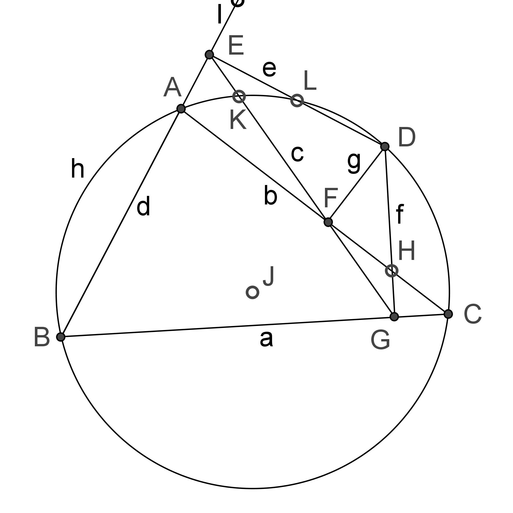
Figure 2: Geometric objects recognized from Fig. 1

A geometric relation is said to be characteristic if all the points used in the relation are characteristic points. To generate candidate propositions for a diagram we are mainly concerned with characteristic points and relations. First of all, we introduce the following rule to remove irrelevant information retrieved.

Rule 1 (Remove irrelevant information).

Remove from $\mathbb{P}$ points that are not characteristic and remove from $\mathbb{R}$ basic geometric relations that are not characteristic.

The following three strategies may be used to implement the above rule.

Strategy 1 (Count weights of points).

In general, characteristic points have labels assigned in the diagram. The more times a point is used in the retrieved geometric relations, the more likely it is to be characteristic.

To determine which points are potentially characteristic, we weight each point of interest by the number of its repeating occurrences in the retrieved relations. Table 2 shows the weights of the points of interest in Fig. 2 according to the retrieved basic geometric relations listed in the right column.

Table 2: Weights of the points of interest in Fig. 2

Point of interest	Weight
$B$	6
$C$	6
$G$	5
$A$	5
$F$	3
$H$	2
$E$	5
$I$	3
$D$	6
$J$	6
$K$	2
$L$	2

Basic geometric relations
$\mbox{{incident}}(G,\mbox{{segment}}(B,C))$
$\mbox{{incident}}(A,\mbox{{halfline}}(B,I))$
$\mbox{{incident}}(F,\mbox{{segment}}(A,C))$
$\mbox{{incident}}(F,\mbox{{segment}}(E,G))$
$\mbox{{incident}}(H,\mbox{{segment}}(A,C))$
$\mbox{{incident}}(H,\mbox{{segment}}(D,G))$
$\mbox{{incident}}(E,\mbox{{halfline}}(B,I))$
$\mbox{{incident}}(K,\mbox{{segment}}(E,G))$
$\mbox{{incident}}(L,\mbox{{segment}}(E,D))$
$\mbox{{pointOnC}}(B,\mbox{{circle}}(J,157))$
$\mbox{{pointOnC}}(C,\mbox{{circle}}(J,157))$
$\mbox{{pointOnC}}(A,\mbox{{circle}}(J,157))$
$\mbox{{pointOnC}}(D,\mbox{{circle}}(J,157))$
$\mbox{{pointOnC}}(K,\mbox{{circle}}(J,157))$
$\mbox{{pointOnC}}(L,\mbox{{circle}}(J,157))$
$\mbox{{perpendicular}}(\mbox{{segment}}(B,C),\mbox{{segment}}(D,G))$
$\mbox{{perpendicular}}(\mbox{{segment}}(A,C),\mbox{{segment}}(F,D))$
$\mbox{{perpendicular}}(\mbox{{halfline}}(B,I),\mbox{{segment}}(E,D))$

Strategy 2 (Re-represent lines and circles).

The weights of points of interest depend on the representations of lines in $\mathbb{L}$ and circles in $\mathbb{C}$, while lines and circles may be represented in different ways. For example, in Fig. 2, the half line $d$ can be represented as $\mbox{{halfline}}(B,A)$ or $\mbox{{halfline}}(B,E)$ instead of $\mbox{{halfline}}(B,I)$ because $B$, $A$, $E$, and $I$ are all incident to $d$; the circle can be represented as $\mbox{{circle}}(A,B,C)$ or $\mbox{{circle}}(B,C,D)$ instead of $\mbox{{circle}}(J,157)$ because $B$, $A$, $D$, and $C$ are all on the circle. It is therefore desirable to determine which representation is the best for ruling out the points that are not potentially characteristic. Generally speaking, among the points incident to a line or a circle, the higher weight a point has, the more possible it is to be characteristic. Therefore, we proceed as follows to re-represent geometric objects according to the weights of points.

Table 3 shows the weights of the points of interest and basic geometric relations for Fig. 2 after the re-representation process.

Table 3: Re-representations of lines and circles

Point of interest	Weight
$B$	7
$C$	8
$G$	5
$A$	8
$F$	3
$H$	2
$E$	5
$I$	0
$D$	6
$J$	0
$K$	2
$L$	2

Basic geometric relations
$\mbox{{incident}}(G,\mbox{{segment}}(B,C))$
$\mbox{{incident}}(F,\mbox{{segment}}(A,C))$
$\mbox{{incident}}(F,\mbox{{segment}}(E,G))$
$\mbox{{incident}}(H,\mbox{{segment}}(A,C))$
$\mbox{{incident}}(H,\mbox{{segment}}(D,G))$
$\mbox{{incident}}(E,\mbox{{halfline}}(B,A))$
$\mbox{{incident}}(K,\mbox{{segment}}(E,G))$
$\mbox{{incident}}(L,\mbox{{segment}}(E,D))$
$\mbox{{pointOnC}}(D,\mbox{{circle}}(A,B,C))$
$\mbox{{pointOnC}}(K,\mbox{{circle}}(A,B,C))$
$\mbox{{pointOnC}}(L,\mbox{{circle}}(A,B,C))$
$\mbox{{perpendicular}}(\mbox{{segment}}(B,C),\mbox{{segment}}(D,G))$
$\mbox{{perpendicular}}(\mbox{{segment}}(A,C),\mbox{{segment}}(F,D))$
$\mbox{{perpendicular}}(\mbox{{halfline}}(B,A),\mbox{{segment}}(E,D))$

Strategy 3 (Determine characteristic points and relations).

After geometric objects are re-represented, the points of interest may be partially determined to be points of attraction or characteristic points according to their weights as follows.

Some of the geometric relations in $\mathbb{R}$ may be derivable from other relations in $\mathbb{R}$. We call geometric relations $D_{1},\ldots,D_{s}$ ($1\leq s$) branch relations with respect to other geometric relations $H_{1},\ldots,H_{d}$ ($1\leq d$) if $D_{1},\ldots,D_{s}$ can be easily derived from $H_{1},\ldots,H_{d}$ on a sub-diagram. The formula in the form of $H_{1},\ldots,H_{d}\Rightarrow D_{1},\ldots,D_{s}$ is used to represent that the branch relations $D_{1},\ldots,D_{s}$ are obtained from $H_{1},\ldots,H_{d}$.

In Fig. 4 (a sub-diagram for Butterfly theorem), $C$ is the midpoint of segment $AB$ and segment $DE$. Then the following four relations can be obtained: (1) $\|AC\|=\|CB\|$; (2) $\|DC\|=\|CE\|$; (3) $\|AD\|=\|EB\|$; (4) $\|AE\|=\|DB\|$. It is easy to see that $(1),(2)\Rightarrow(3),(4)$; $(1),(3)\Rightarrow(2),(4)$; $(1),(4)\Rightarrow(2),(3)$.

Similarly, in Fig. 4 (a diagram for Steiner’s theorem), segment $BD$ and segment $CE$ are internal bisectors of $\angle ABC$ and $\angle BCA$ respectively and $F$ is the intersection point of $BD$ and $CE$. Then the following relations can be obtained: (1) $\|AB\|=\|AC\|$; (2) $\|BD\|=\|CE\|$; (3) $\|AE\|=\|AD\|$; (4) $\|BE\|=\|CD\|$. One sees that $(1),(2)\Rightarrow(3),(4)$; $(1),(3)\Rightarrow(2),(4)$; $(1),(4)\Rightarrow(2),(3)$.

Branch relations are usually not used in theorems about the features of the whole diagram. Therefore, we introduce the following rule.

Rule 2 (Remove branch relations).

If $R_{1},\ldots,R_{k}\Rightarrow R_{k+1},\ldots,R_{m}$ ($1\leq k<m$ and $R_{1},\ldots,R_{m}$ are all basic geometric relations in $\mathbb{R}$), then remove $R_{k+1},\ldots,R_{m}$ from $\mathbb{R}$.

Figure 3: Distance relations on the same line

Figure 4: Distance relations on different lines

There may be different branch relations in the same set of geometric relations (see, e.g., Figs. 4 and 4). The following strategy may be used to select appropriate branch relations.

Strategy 4 (Determine branch relations).

Let $\mathbb{\mathbb{E}}$ be the set of distance relations in $\mathbb{R}$.

As discussed in Section 2.3, retrieved geometric relations in $\mathbb{R}$ are basic and from them other new geometric relations can be derived. A geometric relation $R$ is called a derived relation if it is implied by the basic geometric relations $R_{1},\ldots,R_{m}$ $(2\leq m)$. The formula $R_{1},\ldots,R_{m}\mapsto R$ is used to represent that $R$ can be obtained from $R_{1},\ldots,R_{m}$.

Rule 3 (Introduce derived relations).

If $R_{1},\ldots,R_{m}\mapsto R$ and for all $1\leq i\leq m$, $R_{i}\in\mathbb{R}$ and $R\notin\mathbb{R}$, then remove $R_{1},\ldots,R_{m}$ from $\mathbb{R}$ and add $R$ to $\mathbb{R}$.

Strategy 5 (Introduce new geometric objects).

Derived relations can be obtained from the following formulae:

1. $\mbox{{incident}}(C,p),\mbox{{incident}}(C,q)\mapsto C:=\mbox{{intersection}}(p,q)$;

2. $\mbox{{incident}}(C,\mbox{{segment}}(A,B)),AC=CB\mapsto C:=\mbox{{midpoint}}(A,B)$;

3. $\mbox{{incident}}(C,p),\mbox{{perpendicular}}(p,q)\mapsto C:=\mbox{{foot}}(p,q)$.

For example, from the relations in Table 4 and by Rule 3 one can obtain the derived geometric relations listed in Table 5.

Table 5: Characteristic relations derived from relations in Table 4

Characteristic relations
$G:=\mbox{{foot}}(\mbox{{segment}}(B,C),\mbox{{segment}}(D,G))$
$F:=\mbox{{foot}}(\mbox{{segment}}(A,C),\mbox{{segment}}(D,F))$
$E:=\mbox{{foot}}(\mbox{{halfline}}(B,A),\mbox{{segment}}(D,E))$
$\mbox{{incident}}(F,\mbox{{halfline}}(E,G))$
$\mbox{{pointOnC}}(D,\mbox{{circle}}(A,B,C))$

Strategy 6 (Generate candidate propositions).

To formulate a proposition, one needs to determine which geometric relations can be taken as the hypothesis, in which order the relations are introduced in the hypothesis, and which one can be taken as the conclusion.

We first introduce an order $\prec$ on the characteristic points $P_{1},\ldots,P_{n}$ according to the following two rules.

1. If $P_{i}$ is the label for a derived relation, then $P_{j}\prec P_{i}$, where $P_{j}$ is used in the relation and $P_{j}\neq P_{i}$.

2. Otherwise, if the weight of $P_{i}$ is higher than that of $P_{j}$, then $P_{i}\prec P_{j}$.

For example, according to the weights of the characteristic points in Table 4 and the representations of the characteristic relations in Table 5, an order of the characteristic points is $C\prec A\prec B\prec D\prec G\prec E\prec F$.

Based on the order $\prec$ of points, an order $\lessdot$ is induced on characteristic relations (after the above-stated rules have been applied)

$$R_{1}[P_{11},\ldots,P_{1{k_{1}}}],\,R_{2}[P_{21},\ldots,P_{2{k_{2}}}],\,\ldots,\,R_{m}[P_{m1},\ldots,P_{m{k_{m}}}],$$

where $P_{i1},\ldots,P_{i{k_{i}}}$ are $k_{i}$ points used in $R_{i}\leavevmode\nobreak\ (1\leq i\leq m)$ such that $P_{i1}\prec\cdots\prec P_{i{k_{i}}}$, according to the following three rules.

1. If $P_{i{1}}\prec P_{j{1}}$, then $R_{i}[P_{i1},\ldots,P_{i{k_{i}}}]\lessdot R_{j}[P_{j1},\ldots,P_{j{k_{j}}}]$.

2. If there exists a $w$ ($1\leq w<\min\{k_{i},k_{j}\}$) such that for all $t$ ($1\leq t\leq w$) $P_{i{t}}$ is identical to $P_{j{t}}$ and $P_{i(w+1)}\prec P_{j(w+1)}$, then $R_{i}[P_{i1},\ldots,P_{i{k_{i}}}]\lessdot R_{j}[P_{j1},\ldots,P_{j{k_{j}}}]$.

3. Suppose that $k_{i}\leq k_{j}$. If for all $t$ ($1\leq t\leq k_{i}$) $P_{i{t}}$ is identical to $P_{j{t}}$, then $R_{i}[P_{i1},\ldots,P_{i{k_{i}}}]\lessdot R_{j}[P_{j1},\ldots,P_{j{k_{j}}}]$.

The characteristic relations listed in Table 5 are ordered by $\lessdot$ as: $\mbox{{incident}}(D,$ $\mbox{{circle}}(A,B,C))$ $\lessdot$ $F:=\mbox{{foot}}(\mbox{{segment}}(A,C),\mbox{{segment}}(D,F))$ $\lessdot$ $G:=\mbox{{foot}}(\mbox{{segment}}(B,C),\mbox{{segment}}(D,G))$ $\lessdot$ $E:=\mbox{{foot}}(\mbox{{halfline}}(B,A),$ $\mbox{{segment}}(D,E))$ $\lessdot$ $\mbox{{incident}}(F,$ $\mbox{{segment}}(E,G))$.

Given $R_{1}\lessdot R_{2}\lessdot\cdots\lessdot R_{m}$, the hypothesis and conclusion of a candidate proposition are generated according to the following three rules.

1. Any basic relation $R_{i}$ can be taken as the conclusion.

2. If $R_{i}$ and $R_{j}$ are both derived relations with the same label, then either $R_{i}$ or $R_{j}$ can be taken as the conclusion.

3. The geometric relations other than the conclusion may be taken as the hypothesis.

The generated candidate propositions may be represented in the following form: Proposition($T_{k}$, [$R_{1},\ldots,R_{k-1},R_{k+1},\ldots,R_{m}$], [$R_{k}$]), where $1\leq k\leq m$, $T_{k}$ is the name, $R_{1},\ldots,R_{k-1},R_{k+1},\ldots,R_{m}$ the hypothesis, and $R_{k}$ the conclusion of the proposition.

For example, two candidate propositions may be generated for the diagram in Fig. 1:

$$\mbox{Proposition}(\mbox{Simson}_{5},[\mbox{{incident}}(D,\mbox{{circle}}(A,B,C)),F:=\mbox{{foot}}(\mbox{{halfline}}(A,$$

$$C),\mbox{{segment}}(D,F)),G:=\mbox{{foot}}(\mbox{{segment}}(B,C),\mbox{{segment}}(D,G)),E:=$$

$$\mbox{{foot}}(\mbox{{segment}}(B,A),\mbox{{segment}}(D,E))],[\mbox{{incident}}(F,\mbox{{segment}}(E,G))])$$

and

$$\mbox{Proposition}(\mbox{Simson}_{1},[F:=\mbox{{foot}}(\mbox{{halfline}}(A,C),\mbox{{segment}}(D,F)),G:=\mbox{{foot}}$$

$$(\mbox{{segment}}(B,C),\mbox{{segment}}(D,G)),E:=\mbox{{foot}}(\mbox{{segment}}(B,A),\mbox{{segment}}(D,$$

$$E)),\mbox{{incident}}(F,\mbox{{segment}}(E,G))],[\mbox{{incident}}(D,\mbox{{circle}}(A,B,C))]).$$

3.2 Ruling out False Candidates

To verify the truth of a candidate proposition, we use algebraic methods which have been successfully applied to automated geometric theorem proving. For the efficiency of theorem mining, false propositions need be ruled out first, so that each proposition submitted to a theorem prover is a potential theorem.

A counterexample of a proposition is a diagram for which the hypothesis of the proposition holds, but the conclusion of the proposition does not. If a counterexample can be found, then the proposition must not be a theorem. In what follows we present a numeric verification technique, based on the characteristic set method of Wu [24, 22], for finding counterexamples to rule out false propositions.

Algorithm 4 (Proposition verification).

Given a set $\mathfrak{P}=\{\mathcal{P}_{1},\ldots,\mathcal{P}_{l}\}$ of candidate propositions, output a set $\mathfrak{F}$ of propositions that cannot be theorems.

Set $\mathfrak{F}:=\emptyset$.

For each candidate proposition $\mathcal{P}_{t}\leavevmode\nobreak\ (1\leq t\leq l)$, do the following steps.

Step 4.1.

[Algebraization and triangularization]

Step 4.2.

[Instantiating and solving] Let $\mathbf{u}=\{x_{1},\ldots,x_{h}\}\setminus\{x_{p_{1}},\ldots,x_{p_{r}}\}$. Randomly choose a set $\bar{\mathbf{u}}$ of numeric values for the coordinates in $\mathbf{u}$ and determine (all possible) values $\bar{x}_{p_{1}},\ldots,\bar{x}_{p_{r}}$ for the other coordinates $x_{p_{1}},\ldots,x_{p_{r}}$ by solving the equations

$$c_{j}|_{\mathbf{u}=\bar{\mathbf{u}},x_{p_{1}}=\bar{x}_{p_{1}},\ldots,x_{p_{j-1}}=\bar{x}_{p_{j-1}}}=0,\quad j=1,\ldots,r,$$

successively for $x_{p_{1}},\ldots,x_{p_{r}}$.

Step 4.3.

[Numeric checking] Compute the numeric value $\bar{C}$ of $C$ at $\mathbf{u}=\bar{\mathbf{u}}$ and $(x_{p_{1}},\ldots,x_{p_{r}})=(\bar{x}_{p_{1}},\ldots,\bar{x}_{p_{r}})$. If $\bar{C}<\tau_{C}$ (where $\tau_{C}$ is a prespecified tolerance determined on the basis of empirical results) for all the solutions $(x_{p_{1}},\ldots,x_{p_{r}})=(\bar{x}_{p_{1}},\ldots,\bar{x}_{p_{r}})$, then the proposition $\mathcal{P}_{t}$ is a potential theorem. Otherwise, $\mathcal{P}_{t}$ must not be a theorem, so it is added to $\mathfrak{F}$.

3.3 Proving Theorems

Let $\mathcal{T}_{1},\ldots,\mathcal{T}_{s}$ be the candidate propositions obtained after ruling out the set $\mathfrak{F}$ of propositions from $\mathfrak{P}$ by Algorithm 4. Now one can use Wu’s method to prove the candidate propositions automatically.

For each $\mathcal{T}_{d}$ ($1\leq d\leq s$), let $\mathbf{C}$ be the Wu characteristic set computed in step 4.1 of Algorithm 4 with $\mathcal{P}_{t}=\mathcal{T}_{d}$. Then do the following two steps.

Step 4.4.

[Pseudo-division and irreducible decomposition]

Step 4.5.

[Analyzing nondegeneracy conditions] A candidate proposition may be proved to be a theorem, usually under certain inequality conditions. Some of the conditions are needed to ensure that the considered geometric configurations are in generic position (e.g., a triangle referred to in the proposition does not degenerate to a line). Such algebraic nondegeneracy conditions may be translated back into geometric form (see [32]). There are inequality conditions which are not necessarily connected to nondegeneracy. Those conditions are either unnecessary, or produced to make a partially true theorem a theorem, or included to make the statement of the proposition or its algebraic form rigorous.

4 Implementation and Experiments

The effectiveness of the approach we have proposed for automated generation of geometric theorems from images of diagrams depends on the completeness and accuracy of the information retrieved as well as the capability and efficiency of the theorem prover used. In this section we present some experimental results with a preliminary implementation of the approach.

The algorithms described in Section 2 have been implemented in C++. Images of diagrams for testing and character templates were prepared by using GeoGebra [31] which is a dynamic geometry software system for interactive construction of diagrams, annotation of labels for geometric objects, and exportation of images. Circles and lines are detected from the images of diagrams by using functions cvHoughCircles and cvHoughLines2 provided in OpenCV.

Eight parameters $\tau_{l},\tau_{c},\delta,\tau_{p},\tau_{pl},\tau_{pc},\tau_{d},\tau_{a}$ are used to specify tolerances in our approach for retrieving geometric information from images of diagrams. We firstly acquire empirical values $\overline{\tau_{l}},\ldots,\overline{\tau_{a}}$ for $\tau_{l},\ldots,\tau_{a}$ by making experiments on a set of test images with fixed size $400\times 400$. Then, for any given image I of diagram, the tolerances will be automatically adjusted according to the size of I. For example, if the size of I is $W\times H$, then $\tau_{c}$ will be reset to ${\overline{\tau_{c}}\,\min(W,H)}/{400}$ as $\tau_{c}$ is used to determine the equality of Euclidean distances. The parameters $\tau_{l},\tau_{p},\delta,\tau_{pl},\tau_{pc},\tau_{d}$ will be reset similarly, while $\tau_{a}$ will remain to be $\overline{\tau_{a}}$ because $\tau_{a}$ is used to determine the equality of angles which are not affected by image scaling.

The strategies presented in Section 3.1 for automated generation of candidate propositions have been implemented in Java. As the computation of characteristic sets and irreducible triangular decomposition needed in the process of geometric theorem mining and proving are sophisticated and expensive symbolic computation processes, we choose to use Epsilon [29] for the involved polynomial elimination, triangularization, and decomposition and GEOTHER [32] for automated algebraization and proof of geometric theorems and automated interpretation of algebraic nondegeneracy conditions. An interface for transforming the specifications of candidate propositions into the native representations of GEOTHER has been developed.

To test our approach, we have made experiments on the images of diagrams shown in Table LABEL:experiments. The diagrams used for the experiments were selected from [25], provided that the theorems they illustrate can be expressed by using only the basic geometric relations listed in Table 1. Different diagrams may involve different types of basic relations. For example, the diagrams with Nos. 1 and 2 only involve “onLine” relations; the diagrams with Nos. 3, 4, and 5 involve both “onLine” and “dEqual” relations; the diagram with No. 6 involves both “onLine” and “Perp” relations. It is easy to figure out from the results of test on the diagrams the capability of the current implementation of our approach. In Table LABEL:experiments, “Undesired” denotes the number of undesired geometric relations (e.g., those relations which hold occasionally in the input diagram, but do not hold in other diagrams for the same theorem); “Time” is recorded in seconds for information retrieval from the image; “Candidates” denotes the number of generated candidate propositions; and “Theorems” denotes the number of proved theorems.

Table 6: Test results

No.	Image	Undesired	Time	Candidates	Theorems
1		2	0.25	3	3
2		9	0.25	4	3
3		0	0.187	1	1
4		7	0.203	3	3
5		3	0.203	8	0
6		0	0.14	1	1
7		0	0.156	6	6
8		0	0.187	7	4
9		0	0.124	8	7
10		0	0.187	9	0
9-11		0	0.14	5	5
12		0	0.156	42	1
13		1	0.249	8	8
14		0	0.171	6	4
15		0	0.2	2	2
16		0	0.171	2	2
17		0	0.187	4	4
18		1	0.281	7	7
19		10	0.312	3	3
20		4	0.312	7	6
21		11	0.451	10	0
22		5	0.219	8	0
23		27	0.453	9	0

In the test results, some undesired distance relations (such as $\|AI\|=\|JM\|$ for the diagram image of the nine-point circle theorem with No. 18 and $\|FI\|=\|CH\|$ for that of Pappus’ theorem with No. 1) are retrieved due to insufficient accuracy of geometric object recognition under large error tolerance. Generally speaking, over-strict error tolerance may lead to the missing of useful geometric relations for theorems that should be discovered, while under-strict error tolerance may bring some spurious geometric relations. Appropriate trade-off in the selection of error tolerances for different images can help improve the completeness and accuracy of geometric information retrieval.

For some images of diagrams (such as the image for Thébault’s theorem with No. 12), the number of generated candidate propositions is big because some branch relations (e.g., $\|AC\|=\|CE\|,\|AC\|=\|AE\|\Rightarrow\|AE\|=\|CE\|$) are not ruled out. For some other images of diagrams (such as the image for Morley’s theorem with No. 10 and that for Newton’s theorem with No. 22), though candidate propositions are generated successfully, the desired theorems cannot be proved by using algebraic methods. This failure of theorem proving is mainly for the following reasons.

• The automatically generated specifications of candidate propositions are not appropriate enough. For example, one of the generated candidate propositions for the image with No. 10 is Proposition(Morley₁, [$\|EF\|=\|DE\|$, $\angle ABE=\angle EBD$, $\angle EBD=\angle DBC$, $\angle FAE=\angle EAB$, $\angle CAF=\angle FAE$, $\angle BCD=\angle DCF$, $\angle DCF=\angle FCA$, $\|DF\|=\|EF\|$], [$\|DF\|=\|DE\|$]) in which only one relation is selected for the conclusion. The proposition should have been proved to be true because it is obvious that $\|EF\|=\|DE\|$ and $\|DF\|=\|EF\|$ imply $\|DF\|=\|DE\|$. However, symbolic computation with the algebraic relations expressing the hypothesis is so complicated that makes the program run out of memory. The candidate proposition fails to be a theorem because of inappropriate selection of relations for the hypothesis as well as the conclusion.

• The functions in GEOTHER we have used for automatic assignment of coordinates to points and ordering of variables are not well optimized.

Thus the resulting algebraic expressions are much more complicated than what could be produced with human optimization, so the involved algebraic computations are made more complex as well.

5 Related Work

5.1 Geometric Information Retrieval

Many methods have been proposed for shape recognition from images in the last two decades. Some of them have improved the performance of the traditional Hough transform by exploiting gradient information [12] or using more effective voting schemes [11]. Besides Hough transform, random algorithms for the detection of lines and circles have been proposed in [4, 5]. Those algorithms save a certain amount of storage space by first randomly computing a candidate line or circle and then performing an evidence collecting process to further determine whether the line or circle actually exists. Note that most of the shape detection methods are used to extract rough shapes of objects’ edges from general images. Their accuracy of recognition is not required to be very high. For our purpose of recognizing geometric objects, it is crucial to use OpenCV with numeric data (such as the coordinates of points) to ensure that the accuracy of the detection results is sufficiently high, so that geometric relations implied in images of diagrams can be correctly determined through numeric computation.

5.2 Geometric Theorem Discovery

The reader may consult [6, 8, 9, 17, 20, 21, 24] and references therein for extensive studies on algebraic methods (based on characteristic sets, triangular decomposition, and Gröbner bases) for automated proving and discovering of geometric theorems. Here as examples we mention the open web-based tool [3] developed for automatic discovery of theorems and relations in elementary Euclidean geometry and the deductive database approach [7] proposed for searching all the properties implied in given geometric configurations. In comparison with the existing work, the capability of discovering nontrivial theorems or deductive relations on geometric relations mined automatically from given images of diagrams reflects the novelty of our approach.

5.3 Other Related Work

Besides coordinate-based algebraic methods, other methods for automated theorem proving can also be incorporated into our approach to verify the truth of candidate propositions. Such methods include the area method, the full-angle method, the bracket algebra method, methods based on Clifford algebra, axiom-based deductive methods, and diagrammatic reasoning methods (see [2, 6, 21] and references therein). Some dynamic geometry software systems have implemented specialized methods (e.g., randomized proving methods in Cinderella [14]) to prove theorems for constructed diagrams, or interfaces with geometric theorem provers for generating proofs diagrammatically [23, 26] and exploring knowledge in repositories of geometric constructions and proofs [19]. A web-based library of problems in geometry is being created for testing and evaluating methods and tools of automated theorem proving [18]. A new computational model for computer assisted construction and reasoning of origami has been well studied and used for proving some complicated theorems [13]. Recently, proof assistants have been used to interactively construct and verify proofs in geometry (see, e.g., [15]) and formal systems have established faithful models of proofs from Euclid’s Elements, making use of diagrammatic reasoning (see, e.g., [1]).

6 Conclusion and Future Work

The approach proposed in this paper opens up a completely new route for geometric knowledge discovery and reasoning: retrieve characteristic information (geometric objects and their relations) from simple and inexact data (images of diagrams), generate potential knowledge (candidate propositions) from the retrieved information, and discover profound knowledge (geometric theorems) and validate it by means of automated reasoning (geometric theorem proving). The success of our approach demonstrates the feasibility of automatically acquiring formalized geometric knowledge in quantity from a large scale of images of diagrams available in electronic documents and resources and of efficiently managing such knowledge in a retrievable structure with diagrams instead of ambiguous statements in natural languages.

Our work is still ongoing. More experiments are being carried out and more techniques and strategies are being developed to improve the accuracy of retrieving geometric information from images of diagrams and of ruling out branch relations and introducing derived relations, to generate appropriate specifications of candidate propositions heuristically, and to enhance the efficiency of geometric theorem proving with optimal assignment of coordinates to points.

Currently, the images for experiments are produced from accurate diagrams drawn by using dynamic geometry software. We will extend our approach to deal with scanned and photographed images of hand-drawn diagrams in which the implied geometric relations are inexact. In this case, the retrieval of geometric information becomes more difficult and requires more specialized techniques. The outcome of our study is expected to have practical applications in those areas where geometric information retrieval, knowledge discovery and management, and education are of concern.

References

- [1] J. Avigad, E. Dean, and J. Mumma: A formal system for Euclid’s Elements. The Review of Symbolic Logic 2(4):700–768 (2009)
- [2] P. Balbiani and L. Fariñas del Cerro: Diagrammatic reasoning in projective geometry. In: Logic, Language and Reasoning (H.J. Ohlbach and U. Reyle, eds.), Trends in Logic 5, pp. 99–114, Kluwer, Dordrecht (1999)
- [3] F. Botana: A web-based intelligent system for geometric discovery. In: Computational Science – ICCS 2003, LNCS 2657, pp. 801–810, Springer, Berlin Heidelberg (2003)
- [4] T.C. Chen and K.L. Chung: A new randomized algorithm for detecting lines. Real-Time Imaging 7(6):473–481 (2001)
- [5] T.C. Chen and K.L. Chung: An efficient randomized algorithm for detecting circles. Computer Vision and Image Understanding 83(2):172–191 (2001)
- [6] S.-C. Chou and X.-S. Gao: Automated reasoning in geometry, Handbook of Automated Reasoning, Volume I, Elsevier, North Holland (2001)
- [7] S.-C. Chou, X.-S. Gao, and J.-Z. Zhang: A deductive database approach to automated geometry theorem proving and discovering. Journal of Automated Reasoning 25(3): 219–246 (1996)
- [8] S.-C. Chou and D. Lin: Wu’s method for automated geometry theorem proving and discovering. In: Mathematics mechanization and applications (X.-S. Gao and D. Wang, eds.), pp. 125–146. Academic Press, London (2000)
- [9] G. Dalzotto and T. Recio: On protocols for the automated discovery of theorems in elementary geometry. Journal of Automated Reasoning 43(2):203–236 (2009)
- [10] R.O. Duda and P.E. Hart: Use of the Hough transformation to detect lines and curves in pictures. Communications of Association for Computing Machinery 15(1):11–15 (1972)
- [11] L.A.F. Fernandes and M.M. Oliveira: Real-time line detection through an improved Hough transform voting scheme. The Journal of the Pattern Recognition Society 41(1): 299–314 (2005)
- [12] C. Galambos, J. Kittler, and J. Matas: Gradient based progressive probabilistic Hough transform. Vision, Image and Signal Processing 148(3):158–165 (2001)
- [13] T. Ida, A. Kasem, F. Ghourabi, and H. Takahashi: Morley’s theorem revisited: Origami construction and automated proof. Journal of Symbolic Computation 46(5):571–583 (2011)
- [14] U. Kortenkamp: Foundations of dynamic geometry. Ph.D. thesis, pp. 60–72, ETH Zürich (1999)
- [15] N. Magaud, J. Narboux, and P. Schreck: Formalizing projective plane geometry in Coq. In: Automated Deduction in Geometry, LNAI 6301, pp. 141–162. Springer, Berlin Heidelberg (2011)
- [16] J. Matas, C. Galambos, and J. Kittler: Robust detection of lines using the progressive probabilistic Hough transform. Computer Vision and Image Understanding 78(1):119 C-137 (2000)
- [17] A. Montes and T. Recio: Automatic discovery of geometry theorems using minimal canonical comprehensive Gröbner systems. In: Automated Deduction in Geometry, LNAI 4869, pp. 113–138. Springer, Berlin Heidelberg (2007)
- [18] P. Quaresma: Thousands of geometric problems for geometric theorem provers (TGTP). In: Automated Deduction in Geometry, LNAI 6877, pp. 169–181. Springer, Berlin Heidelberg (2011)
- [19] P. Quaresma and P. Janičić: GeoThms — A web system for Euclidean constructive geometry. Electronic Notes in Theoretical Computer Science 174(2):35–48 (2007)
- [20] D. Wang: Elimination procedures for mechanical theorem proving in geometry. Annals of Mathematics and Artificial Intelligence 13(1–2):1–24 (1995)
- [21] D. Wang: Geometry machines: from AI to SMC. In: Artificial Intelligence and Symbolic Mathematical Computation (J. Calmet, J.A. Campbell, and J. Pfalzgraf, eds.), LNCS 1138, pp. 213–239. Springer, Berlin Heidelberg (1996)
- [22] D. Wang: Elimination methods. Springer, Wien New York (2001)
- [23] S. Wilson and J.D. Fleuriot: Combining dynamic geometry, automated geometry theorem proving and diagrammatic proofs. In: Proceedings of the European Joint Conferences on Theory and Practice of Software (ETAPS), Satellite Workshop on User Interfaces for Theorem Provers (UITP), Edinburgh, UK (2005)
- [24] W.-t. Wu: Mechanical theorem proving in geometries: Basic principles (translated from the Chinese by X. Jin and D. Wang). Springer, Wien New York (1994)
- [25] K. Yano: The famous theorems of geometry (Chinese edition, translated by Y. Chen). Shanghai Scientific and Technical Publishers (1986)
- [26] Z. Ye, S.-C. Chou, and X.-S. Gao: Visually Dynamic Presentation of Proofs in Plane Geometry. Journal of Automated Reasoning 45(3):213–241 (2010)
- [27] H.K. Yuen, J. Princen, J. Illingworth, and J. Kittler: Comparative study of Hough transform methods for circle finding. Image and Vision Computing 8(1):71–77 (1990)
- [28] T.Y. Zhang and C.Y. Suen: A fast parallel algorithm for thinning digital patterns. Communications of the Association for Computing Machinery 27(3):236–239 (1984)
- [29] Epsilon, http://www-polsys.lip6.fr/~wang/epsilon/. Accessed May 23 2014
- [30] Gaussian smoothing, http://en.wikipedia.org/wiki/Gaussian_blur. Accessed May 23 2014
- [31] GeoGebra, http://www.geogebra.org/cms/. Accessed May 23 2014
- [32] GEOTHER, http://www-polsys.lip6.fr/~wang/GEOTHER/. Accessed May 23 2014
- [33] List of interactive geometry software, http://en.wikipedia.org/wiki/List_of_interactive_geometry_software. Accessed May 23 2014
- [34] OpenCV, http://opencv.org/. Accessed May 23 2014