Pseudomagnetic fields in graphene nanobubbles of constrained geometry: A molecular dynamics study

Abstract

Analysis of the strain-induced pseudomagnetic fields generated in graphene nanobulges under three different substrate scenarios shows that, in addition to the shape, the graphene-substrate interaction can crucially determine the overall distribution and magnitude of strain and those fields, in and outside the bulge region. We utilize a combination of classical molecular dynamics, continuum mechanics, and tight-binding electronic structure calculations as an unbiased means of studying pressure-induced deformations and the resulting pseudomagnetic field distribution in graphene nanobubbles of various geometries. The geometry is defined by inflating graphene against a rigid aperture of a specified shape in the substrate. The interplay among substrate aperture geometry, lattice orientation, internal gas pressure, and substrate type is analyzed in view of the prospect of using strain-engineered graphene nanostructures capable of confining and/or guiding electrons at low energies. Except in highly anisotropic geometries, the magnitude of the pseudomagnetic field is generally significant only near the boundaries of the aperture and rapidly decays towards the center of the bubble because under gas pressure at the scales considered here there is considerable bending at the edges and the central region of the nanobubble displays nearly isotropic strain. When the deflection conditions lead to sharp bends at the edges of the bubble, curvature and the tilting of the $p_{z}$ orbitals cannot be ignored and contributes substantially to the total field. The strong and localized nature of the pseudomagnetic field at the boundaries and its polarity-changing profile can be exploited as a means of trapping electrons inside the bubble region or of guiding them in channel-like geometries defined by nano-blister edges. However, we establish that slippage of graphene against the substrate is an important factor in determining the degree of concentration of pseudomagnetic fields in or around the bulge since it can lead to considerable softening of the strain gradients there. The nature of the substrate emerges thus as a decisive factor determining the effectiveness of nanoscale pseudomagnetic field tailoring in graphene.

I Introduction

Since the discovery of a facile method for its isolation, graphene  Novoselov et al. (2005), the simplest two-dimensional crystal, has attracted intense attention not only for its unusual physical properties Geim and Novoselov (2007); Castro Neto et al. (2009); Han et al. (2007); Seol et al. (2010), but also for its potential as the basic building block for a wealth of device applications. There exist key limitations that appear to restrict the application of graphene for all-carbon electronic circuits: one such limitation is that graphene, in its pristine form, is well known to be a semi-metal with no band gap Castro Neto et al. (2009). A highly active field of study has recently emerged based on the idea of applying mechanical strain to modify the intrinsic response of electrons to external fields in graphene  Guinea et al. (2010a); Qi et al. (2013); Tomori et al. (2011). This includes the strain-induced generation of spectral (band) gaps and transport gaps, which suppress conduction at small densities. In this context, several groups  Guinea et al. (2010b); Pereira and Castro Neto (2009); Guinea and Low (2010); Guinea et al. (2008); Abedpour et al. (2011); Guinea et al. (2010a); Kim et al. (2011); Yeh et al. (2011); Yang (2011); Kitt et al. (2012, 2013a); Yue et al. (2012) have employed continuum mechanics coupled with effective models of the electronic dynamics to study the generation of pseudomagnetic fields (PMFs) in different graphene geometries and subject to different deformations. The potential impact of strain engineering beyond the generation of bandgaps has also attracted tremendous interest Pereira and Castro Neto (2009); Pereira et al. (2010a); Abanin and Pesin (2012); Wang et al. (2011).

Pereira et al. (2009) showed that a band gap will not emerge under simple uniaxial strain unless the strain is larger than roughly 20 %. This theoretical prediction, based on an effective tight-binding model for the electronic structure, has been subsequently confirmed by various more elaborate ab-initio calculations Ni et al. (2009); Farjam and Rafii-Tabar (2009); Choi et al. (2010). The robustness of the gapless state arises because simple deformations of the lattice lead only to local changes of the position of the Dirac point with respect to the undeformed lattice configuration Kane and Mele (1997); Suzuura and Ando (2002) and to anisotropies in the Fermi surface and Fermi velocity Pereira et al. (2010b). The shift in the position of the Dirac point is captured, in the low-energy, two-valley, Dirac approximation, by a so-called pseudomagnetic vector potential and resulting pseudomagnetic field (PMF) that arises from the strain-induced perturbation of the tight-binding hoppings Suzuura and Ando (2002). As a result, electrons react to mechanical deformations in a way that is analogous to their behavior under a real external magnetic field, except that overall time-reversal symmetry is preserved, since the PMF has opposite signs in the two time-reversal related valleys Castro Neto et al. (2009).

Guinea et al. (2010a) found that nearly homogeneous PMFs could be generated in graphene through triaxial stretching, but the resulting fields were found to be moderate, unless relatively large (i.e., $>$10 %) tensile strains could be applied. Unfortunately, such large planar tensile strains have not been experimentally realized in graphene to date. This is arguably attributed to the record-high tensile modulus of graphene and the unavoidable difficulty in effectively transferring the required stresses from substrates to this monolayer crystal Gong et al. (2010).

It is thus remarkable that recent experiments report the detection of non-uniform strain distributions in bubble-like corrugations that generate PMFs locally homogeneous enough to allow the observation of Landau quantization by local tunneling spectroscopy. The magnitude of the PMFs reported from the measured Landau level spectrum reaches hundreds (300 to 600) of Teslas Levy et al. (2010); Lu et al. (2012), providing a striking glimpse of the impact that local strain can potentially have on the electronic properties. A difficulty with these experiments is that, up to now, such structures have been seen and/or generated only in contact with the metallic substrates that are used in the synthesis of the sample. This is an obstacle, for example, to transport measurements, since this would require the transfer of the graphene sheet to another substrate, thereby destroying the favorable local strain distribution. In addition, a systematic study of different graphene bubble geometries and substrate types, which could reveal the subtleties that different geometries bring to the related strain-induced PMFs has not been reported. Furthermore, most previous studies of the interplay between strain and electronic structure in graphene have addressed the deformation problem from an analytic continuum mechanics point of view, with the exception of a few recent computational studies Neek-Amal and Peeters (2012a); Neek-Amal et al. (2012).

It is in this context that we report here results from classical molecular dynamics (MD) simulations of strained graphene nanobubbles induced by gas pressure. The MD simulations are used to complement and compare continuum mechanics approaches to calculating strain, in order to examine the pressure-induced PMFs in ultra-small graphene nanobubbles of diameters on the order of 5 nm. Controlled synthesis of such small strained nanobubbles has gained impetus following the recent experiments by Lu et al. Lu et al. (2012). Our aim is to use an unbiased calculation for the mechanical response of graphene at the atomistic level, on the basis of which we can (i) extract the relaxed lattice configurations without any assumptions; (ii) calculate the PMF distribution associated with different nanobubble geometries; (iii) discuss the influence of substrate and aperture shape on PMF distribution; (iv) identify conditions under which explicit consideration of the curvature is needed for a proper account of the PMFs.

We first describe the simulation methodology that was employed to determine the atomic displacements from which the strain tensor, modified electronic hopping amplitudes, and PMFs can be obtained. This is followed by numerical results of the strain-induced PMFs for different graphene nanobubble geometries in a simply clamped scenario. We next discuss the considerable importance of the substrate interaction and, finally, analyze the relative contributions of orbital bending and bond stretching to the total PMF.

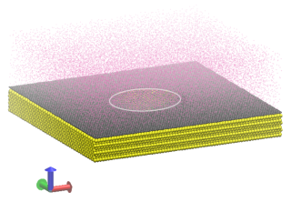
Figure 1: (Color online) Illustration of the strategy employed in our studies to generate nanobubbles by pressurizing graphene through a predefined substrate aperture. The picture shows one of the actual simulation cells used in our MD computations. In gold, gray and red colors are represented, respectively, the Au substrate, the graphene sheet and the Ar atoms. A hole is carved in the Au substrate (perimeter outlined), and its perimeter geometry determines the shape of the resulting graphene bubble. Visualization is performed using VMD Humphrey et al. (1996).

II Simulation methodology

Recent experiments have shown that graphene nanobubbles smaller than 10 nm can be prepared on metallic substrates, and that large PMFs in the hundreds of Tesla result from the locally induced non-homogeneous strain  Levy et al. (2010); Lu et al. (2012). Because such small nanobubbles can be directly studied using classical MD simulations, we employ MD to obtain the deformed graphene bubble configurations due to an externally applied pressure.The atomistic potentials that describe the carbon-carbon interactions have been extensively investigated and, hence, graphene’s nano-mechanics can be simulated without any particular bias, and to a large accuracy within MD. Once the deformation field is known from the simulations, we obtain the strain distribution in the inflated nanobubble, finally followed by a continuum gauge field approach to extract the resulting PMF distribution  Castro Neto et al. (2009); Guinea et al. (2010a, b); Guinea and Low (2010); Guinea et al. (2008); Abedpour et al. (2011).

II.1 Details of the MD simulations

Our MD simulations were done with the Sandia-developed open source code LAMMPS Lammps (2012); Plimpton (1995). The graphene nanobubble system consisted of three parts, as illustrated in Fig. 1: a graphene monolayer, the hexagonal (111) surface of an FCC gold substrate, and argon gas which was used to inflate the graphene bubble. We used the AIREBO potential Stuart et al. (2000) to describe the C-C interactions, as this potential has been shown to describe accurately the various carbon interactions including bond breaking and reforming Zhao and Aluru (2010); Qi et al. (2010). The substrate-graphene and gas-graphene interactions were modeled by a standard 12-6 Lennard-Jones potential:

$$V(r_{ij})=4\,\epsilon_{ij}\left[\left(\frac{\sigma_{ij}}{r_{ij}}\right)^{12}-\left(\frac{\sigma_{ij}}{r_{ij}}\right)^{6}\right],$$ (1)

where $r_{ij}$ represents the distance between the $i$-th carbon and the $j$-th gold atom.

The dimension of the simulation box was 20$\times$20$\times$8 nm³, and the substrate was comprised of Au atoms with a thickness of 2 nm, or about 2.5 times the cutoff distance of the interatomic potential Neek-Amal and Peeters (2012b). Apertures of different shapes (viz. triangle, rectangle, square, pentagon, hexagon, and circle) were “etched” in the center of the substrate to allow the graphene membrane to bulge inwards due to the pressure exerted by the Ar gas. The whole system was first relaxed for 50 ps, at which time the Ar gas was pushed downward (as in a piston) to exert pressure on the graphene monolayer, causing it to bulge inward in the shape cut-out from the gold substrate. The system is then allowed to equilibrate again under the increased gas pressure. All simulations were carried out at room temperature (300 K) using the Nose-Hoover thermostat Hoover (1985). The choice of Ar in our calculations is not mandatory. Substitution with other molecular species should pose no difficulty, the same being true regarding the substrate, as shown previously in references Neek-Amal and Peeters, 2012b and Neek-Amal et al., 2012.

To elucidate the effect of different substrates on the PMF distributions in the nanobubbles, we perform MD simulations with two different substrates, in addition to performing the simulations with fixed edges and no substrate. Specifically, we used both Au and Cu (111) substrates, where the detailed parameters and descriptions will be discussed in later sections.

After obtaining the graphene bubble, we held the pressure constant for 10 ps to achieve thermal equilibrium. We note that during the entire simulation no gas molecules leaked away from the system, which again demonstrates the experimentally observed atomic impermeability of monolayer graphene Nair et al. (2012); Bunch et al. (2008).

Our simulations are close in spirit to the experiments reported in reference Koenig et al., 2011, but targeting smaller hole apertures due to computation limitation. We note that this method of using gas-pressure to generate the graphene nanobubbles is different from the situations explored in the recent experiments that focus on the PMF distribution Levy et al. (2010); Lu et al. (2012). However, it is in some ways more controllable due to the utilization of a substrate with a distinct pattern coupled with externally applied pressure to force graphene through the patterned substrate to form a bubble with controllable shape and height.

The final (inflated bubble) configuration gives us the basic ingredients needed to extract the strain distribution in the system, as well as the perturbed electronic hopping amplitudes. To calculate the strain directly from the displaced atomic positions we employ what we shall designate as the displacement approach. We note that a previous study Klimov et al. (2012) used a stress approach for a similar calculation. However, the stress approach fails to predict reasonable results in our case, which we attribute to the inability of the virial stresses to properly convey the total stress at each atom of the graphene sheet when the load results from interaction with gas molecules. Furthermore, in the stress approach one assumes a planar (and, in addition, usually linear) stress-strain constitutive relation which leads to errors when large out-of-plane deformations arise, as in the case of the nanobubbles. Further details on the strain calculation are given in appendix D.

II.2 Displacement approach to calculate strain

In continuum mechanics the infinitesimal strain tensor is written in Cartesian material coordinates ($X_{i}$) as

$$\epsilon_{ij}=\frac{1}{2}\left(\frac{\partial{u_{i}}}{\partial{X_{j}}}+\frac{\partial{u_{j}}}{\partial{X_{i}}}\right)+\frac{1}{2}\left(\frac{\partial{u_{k}}}{\partial{X_{i}}}\frac{\partial{u_{k}}}{\partial{X_{j}}}\right)\!\!.$$ (2)

To utilize Eq. 2, it is clear that the displacement field must be obtained such that its derivative can be evaluated to obtain the strain. In order to form a linear interpolation scheme using finite elements Hughes (1987), we exploit the geometry of the lattice and mesh the results of our MD simulation of the deformed graphene bubble using tetrahedral finite elements defined by the positions of four atoms: the atom of interest (with undeformed coordinates $\mathbf{R}_{0}$), and its three neighbors (with undeformed coordinates $\mathbf{R}_{1}$, $\mathbf{R}_{2}$, $\mathbf{R}_{3}$). After deformation, the new positions of the atoms are $\mathbf{r}_{0}$, $\mathbf{r}_{1}$, $\mathbf{r}_{2}$ and $\mathbf{r}_{3}$, respectively. To remove spurious rigid body translation and rotation modes, we took the atom of interest ($\mathbf{R}_{0}$) as the reference position, i.e., $\mathbf{r}_{0}$ = $\mathbf{R}_{0}$. The displacement of its three neighbors could then be calculated, and subsequently the components of the strain tensor $\epsilon_{ij}$ were obtained by numerically evaluating the derivative of the displacement inside the element.

II.3 Pseudomagnetic fields

Non-zero PMFs arise from the non-uniform displacement in the inflated state. These PMF reflect the physical perturbation that the electrons near the Fermi energy in graphene feel as a result of the local changes in bond length. It emerges straightforwardly in the following manner. Nearly all low-energy electronic properties and phenomenology of graphene are captured by a simple single orbital nearest-neighbor tight-binding (TB) description of the $\pi$ bands in graphene Castro Neto et al. (2009). In second quantized form this tight-binding Hamiltonian reads

$$H=-\sum_{i,\mathbf{n}}t\bigl{(}\mathbf{r}_{i},\mathbf{r}_{i}+\mathbf{n}\bigr{)}\,a^{\dagger}_{\mathbf{r}_{i}}b^{\phantom{\dagger}}_{\mathbf{r}_{i}+\mathbf{n}}+\text{H. c.},$$ (3)

where $t\bigl{(}\mathbf{r}_{i},\mathbf{r}_{i}+\mathbf{n}\bigr{)}$ represents the hopping integral between two neighboring $\pi$ orbitals, $\mathbf{n}$ runs over the three nearest unit cells, and $a_{\mathbf{r}_{i}}$($b_{\mathbf{r}_{i}}$) are the destruction operators at the unit cell $\mathbf{r}_{i}$ and sublattice $A(B)$. In the undeformed lattice the hopping integral is a constant: $t\bigl{(}\mathbf{r}_{i},\mathbf{r}_{i}+\mathbf{n}\bigr{)}=t\bigl{(}\mathbf{R}_{i},\mathbf{R}_{i}+\mathbf{n}\bigr{)}=t=2.7$ eV. The deformations of the graphene lattice caused by the gas pressure impact the hopping amplitudes in two main ways. One arises from the local stretch that generically tends to move atoms farther apart from each other and, consequently, directly affects the magnitude of the hopping $t_{ij}$ between neighboring atoms $i$ and $j$, which is exponentially sensitive to the interatomic distance. The other effect is caused by the curvature induced by the out-of-plane deflection, which means that the hopping amplitude is no longer a purely $V_{pp\pi}$ overlap (in Slater-Koster notation) but a mixture of $V_{pp\pi}$ and $V_{pp\sigma}$. More precisely, one can straightforwardly show that the hopping between two $p_{z}$ orbitals oriented along the unit vectors $\mathbf{n}_{i}$ and $\mathbf{n}_{j}$ and a distance $\mathbf{d}$ apart is given by Isacsson et al. (2008); Pereira et al. (2010a)

$$-t_{ij}=V_{pp\pi}(d)\,\mathbf{n}_{i}\cdot\mathbf{n}_{j}\\ +\frac{V_{pp\sigma}(d)-V_{pp\pi}(d)}{d^{2}}\,(\mathbf{n}_{i}\cdot\mathbf{d})(\mathbf{n}_{j}\cdot\mathbf{d})\,.$$ (4)

To capture the exponential sensitivity of the overlap integrals to the interatomic distance $d$ we model them by

$$V_{pp\pi}(d) =-t\,e^{-\beta(d/a-1)},$$ (5a)

$$V_{pp\sigma}(d) =+1.7\,t\,e^{-\beta(d/a-1)},$$ (5b)

with $a\simeq 1.42$ Å the equilibrium bond length in graphene. For static deformations a value $\beta\approx 3$ is seen to capture the distance dependence of $V_{pp\pi}(d)$ in agreement with first-principles calculations Pereira et al. (2009); Pereira et al. (2010b); we use the same decay constant $\beta$ for both overlaps, which is justified from a Mülliken perspective since the principal quantum numbers of the orbitals involved is the same Hansson and Stafström (2003).

In the undeformed state Eq. (4) reduces to $-t_{ij}=V_{pp\pi}(a)\equiv-t$ and is, of course, constant in the entire system. But local lattice deformations cause $t\bigl{(}\mathbf{r}_{i},\mathbf{r}_{i}+\mathbf{n}\bigr{)}$ to fluctuate, which we can describe by suggestively writing $t\bigl{(}\mathbf{r}_{i},\mathbf{r}_{i}+\mathbf{n}\bigr{)}=t+\delta t\bigl{(}\mathbf{r}_{i},\mathbf{r}_{i}+\mathbf{n}\bigr{)}$. In the low energy (Dirac) approximation, the effective Hamiltonian around the point $\mathbf{\pm K}$ in the Brillouin zone can then be written as Kane and Mele (1997); Suzuura and Ando (2002)

$$H_{\text{eff}}^{\pm\mathbf{K}}=v_{F}\,\bm{\sigma}\cdot\bigl{(}\mathbf{p}\mp q\mathbf{A}\bigr{)},$$ (6)

where $\hbar v_{F}=3ta/2$, $q$ represents the charge of the current carriers ($q>0$ for holes and $q<0$ for electrons), and the Cartesian components of the pseudomagnetic vector potential $\mathbf{A}=A_{x}\bm{e}_{x}+A_{y}\bm{e}_{y}$ are given explicitly in terms of the hopping perturbation by

$$A_{x}(\mathbf{R})-iA_{y}(\mathbf{R})=\frac{1}{qv_{F}}\sum_{\bm{n}}\delta t\bigl{(}\mathbf{r},\mathbf{r}+\mathbf{n}\bigr{)}e^{i\bm{K}\cdot\bm{n}}.$$ (7)

For nearly planar deformations (small out-of-plane vs in-plane displacement ratios and thus neglecting bending effects) $\delta t$ can be expanded in terms of the local displacement field and, consequently, can be cast in terms of the strain components. Orienting the lattice so that the zig-zag direction is parallel to $\bm{e}_{x}$ leads to

$$A_{x}(\mathbf{R})-iA_{y}(\mathbf{R})\simeq\frac{\hbar\beta}{2qa}\bigl{(}\epsilon_{xx}-\epsilon_{yy}+2i\,\epsilon_{xy}\bigr{)},$$ (8)

Since we are ultimately interested in the PMF, only the contributions to $\mathbf{A}(\mathbf{R})$ arising from the hopping modification are considered here, as they are the ones that survive after the curl operation de Juan et al. (2013); Kitt et al. (2012, 2013a); Sloan et al. (2013); Oliva-Leyva and Naumis (2013); we also don’t consider contributions beyond second order smallness ($\sim k\,\epsilon$, $\sim k^{2}$, etc.). In the planar strain situation the whole information about the electronic structure is reduced to the parameter $\beta=-\partial\log t(r)/\partial\log r\bigr{|}_{r=a}$.

From the coupling in Eq. (6) where the effects of strain are captured by replacing $\mathbf{p}\to\mathbf{p}-q\mathbf{A}$ it is clear that the local strain is felt by the electrons in the $\bm{K}$ valley in the same way as an external magnetic field would be. In particular, we can quantify this effect in terms of the PMF, which is defined as

$$B=\partial_{x}A_{y}(\mathbf{R})-\partial_{y}A_{x}(\mathbf{R}).$$ (9)

This is the central quantity of interest in this work; in the subsequent sections the combined effects of gas pressure, hole geometry, and substrate interaction will be analyzed from the point of view of the resulting magnitude and space distribution of the PMF, $B$, obtained in this way. For definiteness we set $q=e$, $e$ being the elementary charge, which means that we shall be analyzing the PMF from the perspective of holes ($q>0$). From an operational perspective, $B$ can be calculated directly from Eq. (7) by computing the hopping between all pairs of neighboring atoms in the deformed state, or from Eq. (8) by calculating the strain components throughout the entire system as described in the previous section. The former strategy is here referred to as the TB approach, and the latter as the displacement approach, as per the definitions in section II.2. Our PMF calculations in the following sections are done by following the TB approach, except when we want to explicitly compare the results obtained with the two approaches. In those cases, such as in the next section or in Appendix C, that will be explicitly stated.

III Clamped graphene nanobubbles

We first simulated an idealized system consisting only of Ar gas molecules and graphene, neglecting the interaction with the underlying substrate, and where we strictly fixed all carbon atoms outside the aperture region during simulation. This provides a good starting point to understand how the shape of the substrate aperture affects the PMF distribution. A similar system has been used in previous work Wang et al. (2013), as this corresponds to a continuum model with clamped edges Guinea et al. (2008); Kim et al. (2011).

We start with the most symmetric geometry, a circular graphene bubble, and compare the atomistic result with the continuum Hencky solution Fichter (1997). In contrast to small deformation continuum models Kim et al. (2011), the Hencky model is valid for large in-plane (stretching) deformations, which lead to a different PMF distribution. To compute the PMFs associated with this analytical solution we used Eq. (8). Figs. 2(c,d) show that the PMF distribution is dominated by very large magnitudes at the edges followed by a rapid decay towards the inside region of the nanobubble. Both the MD and Hencky results show the six-fold symmetry expected for a cylindrically symmetric strain distribution; this agreement demonstrates the MD simulation successfully captures the strain distribution underlining the computed PMF. There are, however, two quite clear discrepancies between the PMF in these two figures: (i) Hencky’s solution (panel d) yields values considerably smaller in magnitude than the calculation based on the MD deformations combined with Eqs. (4) and (7) (panel c); (ii) the sign of the PMF in panel (d) is apparently reversed with respect to the sign of panel (c). These discrepancies stem from the substantial bending present in graphene near the hole perimeter, and deserve a more detailed inspection in terms of the relative magnitude of the two contributions to the hopping variation: bond stretching and bond bending.

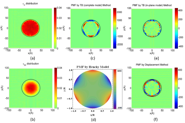
Figure 2: (Color online) Results for a circular graphene bubble with 4 nm radius and pressurized up to $\sim$1 nm deflection; in this case graphene was clamped at the edge of the substrate aperture. (a) Radial strain, (b) tangential strain, (c) PMF by TB method with both in-plane and bending components, (d) PMF arising from Hencky’s analytic model Fichter (1997) with the axes scaled in units of the circle radius, (e) PMF by TB method with in-plane component only, (f) PMF by displacement method. Note that, except for (d), all the panels refer to the same atomistic configuration. PMF in shown in units of Tesla. The edge of the substrate aperture used in the MD simulation is outlined (gray line) for reference.

Since Hencky’s result of Fig. 2(d) hinges on Eq. (8) that expresses the vector potential directly in terms of the strain tensor components, let us start by analyzing the predictions obtained by applying it to the atomistic case as well; to do that one computes the strain from the MD simulations using the displacement approach discussed earlier. The result of that is shown in Fig. 2(f), where the most important difference in comparison with Fig. 2(c) is the significant reduction of the maximal fields obtained near and at the edges; this reflects the error incurred in the quantitative estimate of $B$ when the effect of bending is neglected. Note that, by construction, Eq. (8) accounts only for the bond-stretching, and is accurate only to linear order in strain because it is based on a linear expansion of the hopping in the interatomic distances. Hence, in order to correctly extract from the atomistic simulations the total stretching contribution beyond linear order while still ignoring bending effects, we should calculate the PMF with the hopping as defined in Eq. (4) (TB approach), but explicitly setting $\mathbf{n}_{i}\cdot\mathbf{n}_{j}=1$ and $\mathbf{n}_{i}\cdot\mathbf{d}=0$ (i.e.assuming local flatness). The outcome of this calculation is shown in Fig. 2(e) which, in practical terms, is the counterpart of Fig. 2(c) with bending effects artificially suppressed. In comparison with panel (f), it leads to slightly smaller PMF magnitudes. The linear expansion in strain of Eq. (7) thus slightly overestimates the field magnitudes, something expected because the hopping is exponentially sensitive to the interatomic distance and, by expanding linearly, one overestimates its rate of change with distance, overestimating the field magnitude as a result. One key message from Fig. 2 and the comparison between panel (c) and any of the subsequent ones is that the effects of curvature are significant at these scales of deflection and bubble size, particularly at the edge, where they clearly overwhelm the “in-plane” stretching contribution. We will revisit this in more detail in section VI.

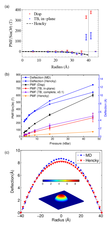
Figure 3: (Color online) (a) Angular-averaged values of $B/\sin(3\theta)$ for the circular nanobubble with $R=4$ nm considered in Fig. 2. The different datasets correspond to different strategies discussed in the main text to obtain the PMF. The vertical line at $r=R\approx 40$ Å marks the radius of the circular aperture in the substrate. For $r<R$ the results extracted from MD closely follow the analytical curve, but there is a sharp sign change and increase at $r\approx R$ (see appendix A for details of the averaging procedure, as well as for the TB data including the full hopping perturbation). (b) Comparison between the pressure-induced deflection and maximum PMF magnitude at the edge, $|\,B(R\approx 40\,\text{\AA})\,|$, obtained with the different approximations discussed in the text. The points corresponding to the complete TB hopping are scaled by 0.1 for better visualization. (c) A section of the simulated nanobubble (MD) at $\sim$19 kBar and the corresponding Hencky’s solution (the inset shows a 3D perspective of the former with the color scale reflecting the vertical displacement).

The second key message gleaned from Fig. 2 pertains to the importance of properly considering the boundary and loading conditions when analytically modeling the strain and deflection of graphene. This is related to the apparent opposite sign in the PMF at the edge obtained from Hencky’s solution in panel (d) when compared with all the other panels (containing the MD-derived results). To elucidate the origin of the difference we show in Fig. 3(a) the PMF divided by the angular factor $\sin(3\theta)$, and averaged over all the angles (details discussed in appendix A). This plot provides a summary of the data in Figs. 2(d,e,f) and allows a cross-sectional view of the variation of the field magnitude with distance from the center of the nanobubble. Direct inspection shows that the averaged MD data follows Hencky’s prediction inside the bubble nearly all the way to the edge, at which point the PMF derived from the atomistic simulations swerves sharply upwards, changes sign, and returns rapidly to zero within one lattice spacing beyond the bubble edge (the curve derived from Hencky’s model terminates at the edge, by construction). This effective sectional view explains why the density plots in Figs. 2(c,d) seem to have an overall sign mismatch: in the MD-derived data, the plots of the PMF distribution are dominated by the large values at the edge which have an opposite sign to the field in the inner region. Fig. 3(a) shows that, rather than a discrepancy, there is a very good agreement between the strain field predicted by Hencky’s solution and a fully atomistic simulation throughout most of the inner region of the nanobubble. However, since Hencky’s solution assumes fixed boundary conditions at the edge (zero deflection, zero bending moment) Fichter (1997), it cannot capture the sharp bends expected at the atomic scale generated by the clamping imposed in these particular MD simulations (in effect, corresponding to zero deflection and its derivative). The finite bending stiffness of graphene Wei et al. (2013) comes into play in that region, generating additional strain gradients which explain the profile and large magnitude of the PMF seen in the atomistic simulations.

In Fig. 3(b) we plot the evolution of the deflection and maximum PMF with increasing gas pressure. The maximum PMF is obtained around the edge of the aperture, and the values shown in the figure correspond to an angular average of the PMF amplitude there (see appendix A for details). The MD and analytical (Hencky’s) solutions give comparable results for the deflection in the pressure range below $<1\times 10^{4}$ bar (Fig. 3(b), right vertical scale). At higher pressures, Figs 3(b) and 3(c) show that the analytical solution yields a slightly smaller deflection, as the underlying model does not capture the nonlinear elastic softening that has been observed in graphene in both experiments Lee et al. (2008) and previous MD simulations Jun et al. (2011). Fig. 3(b) includes also the maximum PMFs occurring at the bubble edge, when computed with the different approaches discussed above in connection with Figs 2(c-f). We highlight that Hencky’s solution cannot generate significant PMFs even at the largest deflections, whereas experiments in similarly sized and deflected nanobubbles easily reveal PMFs in the hundreds of Teslas Levy et al. (2010); Lu et al. (2012). This raises questions about the applicability of the Hencky solution at these small scales and large deflections.

The pressure required to rupture this graphene bubble was determined to be around $1.9\times 10^{5}$ bar from our MD simulations. Such a large value is required because of the small dimensions of the bubble. We can calculate the fracture stress by adopting a simple model for a circular bulge test, i.e., $\sigma\sim\frac{R\delta P}{2w}$, where $\sigma$, $\delta P$, $R$, and $w$ are the stress, pressure difference, radius, and thickness of the membrane, respectively. Assuming $w$ to be 3.42 Å, we obtain a fracture strength of about 80 GPa, which is in agreement with previous theoretical Zhao and Aluru (2010) and experimental Lee et al. (2008); Zhao and Aluru (2010) results. Note that the plot in Fig. 3 shows very large pressures (up to near the rupture limit of the bubble) and correspondingly large deflections since we wish to highlight the points of departure between the elastic model and the simulation results. Pressures and deflections considered in the specific cases discussed below are considerably smaller.

With the good performance of the atomistic model on the circular graphene bubble established, we next extend the analysis to nanobubbles with different shapes. The bubbles are similarly obtained by inflation of graphene under gas pressure against a target hole in the substrate with the desired shape. Fig. 4 shows results of a study of different shapes to which the displacement interpolation approach was applied to obtain the strain field and, thus, the PMFs. The shapes are a square, a rectangle (aspect ratio of 1:2), a pentagon, a hexagon, and a circle, and are presented in order of approximately decreasing symmetry. Those geometries are chosen because they are sufficiently simple that they can be readily fabricated experimentally with conventional etching techniques. The dimensions of the different bubbles were chosen such that their areas were approximately $\sim$50 nm². The pressure was 19000 bar and side lengths for the bubble geometries shown in Figs. 4(a)-4(f) were, respectively, 4 nm (circle), 4.4 nm (hexagon), 5.7 nm (pentagon), 5 nm (rectangle, short edge), 7.1 nm (square), 10.6 nm (triangle).

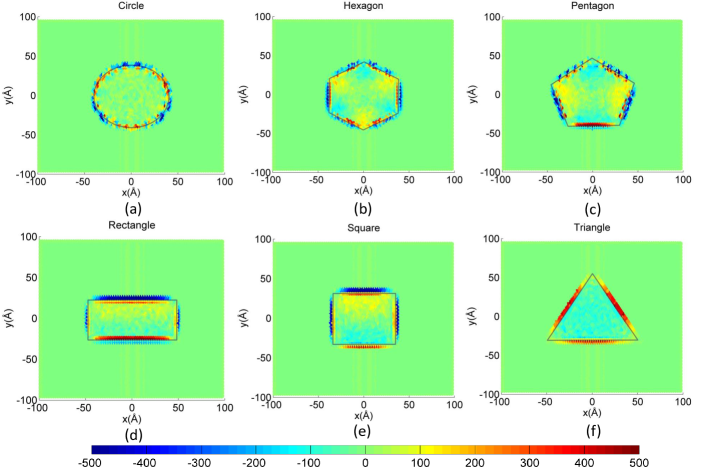
Figure 4: (Color online) Top views of PMF patterns for graphene bubbles of different geometries without substrate. (a) circle (b) hexagon (c) pentagon (d) rectangle (aspect ratio 1:2) (e) square (f) triangle. All the bubble areas are $\sim 50\,\text{nm}^{2}$, and side lengths and pressures can be found in the main text. In all cases, the graphene lattice is oriented with the zig-zag direction along the horizontal. The same color scale (in Tesla) is used in all panels. The edge of the substrate apertures used in the MD simulations is outlined (gray line) for reference.

It is worth emphasizing that these features depend on the orientation of the graphene lattice with respect to the substrate aperture, as we would expect. This is clearly visible in the case of the square bubble in Fig. 4(e), for which the sharp magnetic field along the boundary is present along the horizontal (zig-zag) edges of the bubble but not along the vertical ones (armchair). This is also the reason why only the triangular aperture shown in Fig. 4(f) leads to a strong PMF that is nearly uniform as one goes around the boundary of the nanobubble. This is an important consideration for the prospect of engineering strained graphene nanostructures capable of guiding or confining electrons within, much like a quantum dot Qi et al. (2013). The sharp PMF at the boundary acts effectively as a strong magnetic barrier, which might be tailored to confine some of the low energy electronic states De Martino et al. (2007); Masir et al. (2009); Klimov et al. (2012).

The resulting PMF patterns in Fig. 4 show that the highest values are found at the corners and edges of the different bubble shapes. To illustrate more clearly the PMF patterns, we inflated the bubbles to large deflections ($\sim$1 nm) with strains reaching 10 % and the corresponding pressure exceeding $1\times 10^{4}$ bar. These large deflections explain why the PMF magnitudes in Fig. 4 may reach over 500 T. Given that the gas pressures used to achieve the results shown in this figure are rather high, some comments are in order.

First, we emphasize that the relevant parameter is the deflection, rather than the pressure itself. In other words, gas pressure was employed here as one way of generating graphene nanobubbles with predefined boundary geometries and target deflections, but other loading conditions might be used to achieve the same parameters. Our choice is motivated by the desire to constrain graphene and its interaction with the substrate as little as possible. Since we intend to reproduce bubbles with lateral size and deflections matching the magnitude of the values observed experimentally Levy et al. (2010); Lu et al. (2012) this requires large pressures (for a given target deflection $P$ is naturally smaller for larger apertures). Secondly, Lu et al. (2012) reported that experimental bond elongations, estimated from direct STM mapping of the atomic positions and deflections, can exceed 10 % in graphene nanobubbles on Ru. The high pressures considered in our MD simulations allow us to reach bond elongations of this order of magnitude. Thirdly, pressures of the order of $10$ kbar (1 GPa) have been recently estimated to occur within nanobubbles of similar dimensions and deflections to the ones considered here, formed upon annealing of graphene-diamond interfaces Lim et al. (2012). Thus, pressures of this magnitude are not unrealistic in the context of nanoscale graphene blisters.

IV Substrate interaction: Graphene on Au (111)

Having considered the ideal case of graphene without a substrate, we move forward to study the more realistic case of graphene lying on an Au (111) substrate. The main difference is that the carbon atoms are not rigidly attached to the substrate anymore outside the aperture, meaning that graphene can slide into the aperture during inflation, subject to the interaction with the substrate. This is an important qualitative difference, and reflects more closely the experimental situation, as recently reported in reference Kitt et al., 2013b. The interatomic interactions were parameterized with $\epsilon_{C-Au}$=0.02936 eV, $\sigma_{C-Au}$=2.9943 Å Piana and Bilic (2006); $\epsilon_{C-Ar}$=0.0123 eV, $\sigma_{C-Ar}$=3.573 Å Tuzun et al. (1996); $\epsilon_{Ar-Ar}$=0.0123 eV, $\sigma_{Ar-Ar}$=3.573 Å Rytkönen et al. (1998); the Ar-Au (gas-substrate) interactions were neglected to save computational time, and the substrate layer was held fixed for the entire simulation process. Most of the graphene layer was unconstrained, except for a 0.5 nm region around the outer edges of the simulation box where it remained pinned. Since the interaction with the substrate is explicitly taken into consideration, this approach realistically describes the sliding and sticking of graphene on the substrate as the gas pressure is increased, as well as details of the interaction with the substrate in and near the hole perimeter.

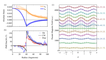
Figure 5: (Color online) (a) Strain components $\epsilon_{rr}$ and $\epsilon_{\theta\theta}$ of a graphene bubble pressurized to a deflection of $\sim 1$ nm against a circular hole with 4 nm radius on a Au(111) substrate. (b) The corresponding PMF along the radial direction from the bubble center computed according to the extended Hencky model Kitt et al. (2013b) (solid line) and from MD simulations within the TB (blue) or displacement (red) approach. Panel (d) shows the angular dependence of the PMF for selected radii.

We start the discussion with a direct comparison of the deformation state of a circular bubble obtained from our simulations with the predictions of a recently developed and experimentally verified ‘extended-Hencky’ model Kitt et al. (2013b) that accounts for the same sliding and friction effects. As can be seen in Fig. 5(a), after fitting the friction in the continuum model to the MD simulation there is a very good agreement between the MD and extended Hencky results for the radial and tangential strains, $\epsilon_{rr}$ and $\epsilon_{\theta\theta}$, both in the inner and outer regions with respect to the substrate aperture. The same good agreement is seen in the PMF profile extracted from the MD and analytical approaches, which is presented in Fig. 5(b). The numerical data points shown in this panel represent an angular average over an annulus centered at different radii. An important message from Fig. 5(b) is that the maximum magnitude of the PMF occurs around the edge of the aperture, but on the outside of the bubble. Whereas one expects the maximal PMFs to occur around the edge where the strain gradients are larger, the fact that the magnitude is considerably higher right outside rather than inside is not so obvious. This has important implications for the study of PMFs in graphene nanostructures but has been ignored by previous studies. It implies that models where only the deflection inside the aperture is considered (such as the simple Hencky model) can miss important quantitative and qualitative features. They are captured here because the friction and sliding effects due to graphene-substrate interactions are naturally taken into account from the outset. One consequence is the “leakage” of strain outside the bubble region and the concurrent emergence of PMFs outside the aperture. This should be an important consideration in designing nanoscale graphene devices with functionalities that rely on the local strain or PMF distribution.

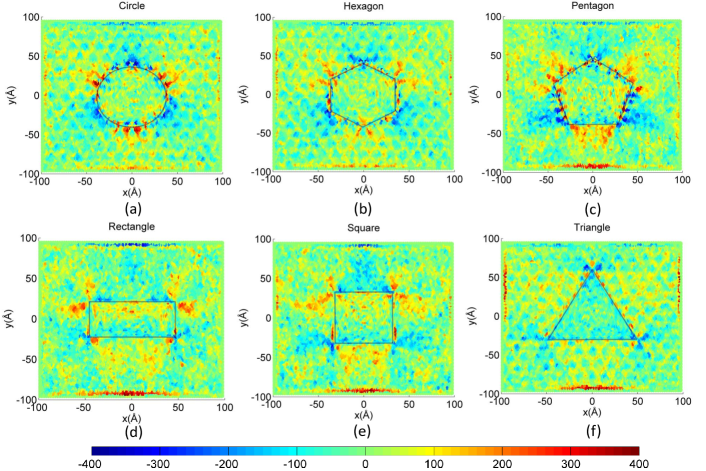
Figure 6: (Color online) Top views of PMF patterns for graphene bubbles of different geometries on Au (111) substrates. (a) circle (b) hexagon (c) pentagon (d) rectangle (aspect ratio 1:2) (e) square (f) triangle. All the bubble areas are $\sim 50\,\text{nm}^{2}$, and side lengths and pressures can be found in the main text. In all cases, the graphene lattice is oriented with the zig-zag direction along the horizontal. The same color scale (in Tesla) is used in all panels. The edge of the substrate apertures used in the MD simulations is outlined (gray line) for reference.

The other shapes studied on the Au (111) substrate are shown in Fig. 6. The dimensions are the same as in Fig. 4, with an applied pressure of $\sim$ 30 kbar. In addition to the appearance of non-negligible PMF outside the aperture region, a comparison with the data for bubbles clamped to the hole perimeter shows that now the PMF distribution inside is noticeably perturbed, and that the large field magnitudes observed in Fig. 4 along the perimeter are considerably reduced and smoother.

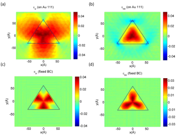
Figure 7: (Color online) Spatial patterns of the strain tensor components $\epsilon_{rr}$ and $\epsilon_{\theta\theta}$ for a triangular bubble with a 10.6 nm side. (a) and (b) pertain to graphene on a Au (111) substrate whose PMF profile has been shown in Fig. 4(f), while (c) and (d) correspond to the graphene bubble with an artificially fixed boundary condition whose PMF is shown in Fig. 6(f). The edge of the substrate aperture used in the MD simulation is outlined (gray line) for reference.

To understand the origin of this difference, let us analyze in detail the representative case of a triangular nanobubble, as previous experiments have shown that such nanobubbles can exhibit PMFs in excess of 300 T Levy et al. (2010). Using our MD-based simulation approach, we calculate the PMFs for triangular graphene bubbles by inflating a graphene monolayer through a triangular hole in the substrate. The set-up is as illustrated in Fig. 1, but with the circular hole replaced by a triangular one. The triangular hole in the substrate had a side length of 10.6 nm, and the graphene sheet was inflated to a deflection of $\sim$ 1 nm. The resulting PMF distribution when one artificially clamps graphene outside the hole region has been shown in Fig. 4(f); the underlying strain components can be seen in Figs. 7(c,d). Upon inflation under the gas pressure, the geometry and the clamped conditions enforce an effective tri-axial stretching in the graphene surface that is clearly visible in the strain distribution. As pointed out by Guinea et al. (2010a), this tri-axial symmetry is crucial for the experimental observation of Landau levels in reference Levy et al., 2010 because it leads to a quasi-uniform PMF inside the nanobubble. Inspection of Fig. 4(f) confirms that the field is indeed of significant magnitude and roughly uniform within the bubble.

When the full interaction with the substrate is included and the graphene sheet is allowed to slip and slide towards the aperture under the inflation pressure, the geometry is no longer as effective as before in generating a clear triaxial symmetry: a comparison of the top and bottom rows of Fig. 7 shows that the triaxial symmetry of the strain distribution is not so sharply defined in this case. Therefore, the finite and roughly uniform PMF inside the triangular boundary that is seen clearly in Figs. 4(f) [and also Figs. 16(f)] is largely lost here. To understand the difference we start by pointing out that the orientation of the triangular hole with respect to the crystallographic axes used here is already the optimum orientation in terms of PMF magnitude, with its edges perpendicular to the $\langle 100\rangle$ directions (i.e., parallel to the zig-zag directions). Secondly, since the graphene sheet is allowed to slide, the strain distribution in the central region of the inflated bubble tends to be more isotropic, as we expect for an inflated membrane because of the out of plane displacement, and as can be seen in Fig. 7. This means that the trigonal symmetry imposed on the overall strain distribution by the boundaries of the hole is less pronounced near the center. As a result, even though strain increases as one moves from the edge towards the center (as measured, for example, by looking at the bond elongation directly from our MD simulations), the magnitude of the PMF decreases because the trigonal symmetry and strain gradients become increasingly less pronounced, and we know that the isotropic (circular) hole yields zero PMF at the apex (Fig. 2).

The differences in trend and the sensitivity of the PMF distribution to the details of the interaction with the substrate highlight the importance of the latter in determining the final distribution and magnitude of the PMF, in addition to the loading, hole shape, and boundary conditions. In order to stress this aspect, and to make the role of the substrate interaction even more evident, we shall consider next a different metal surface.

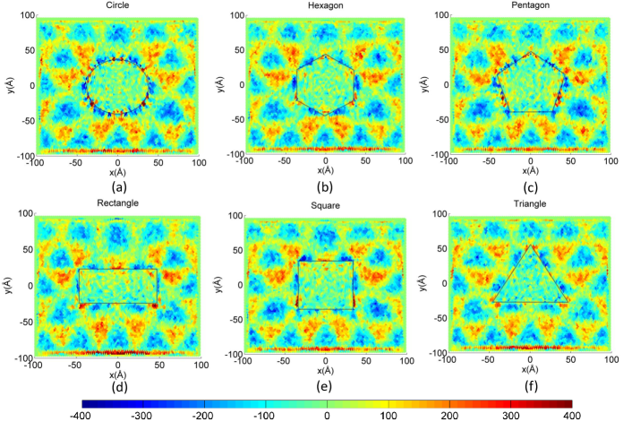
Figure 8: (Color online) Top views of PMF patterns for graphene bubbles of different geometries on Cu (111) substrate. (a) circle (b) hexagon (c) pentagon (d) rectangle (aspect ratio 1:2) (e) square (f) triangle. All the bubble areas are $\sim 50\,\text{nm}^{2}$, and side lengths and pressures can be found in the main text. In all cases, the graphene lattice is oriented with the zig-zag direction along the horizontal. The same color scale (in Tesla) is used in all panels. The edge of the substrate apertures used in the MD simulations is outlined (gray line) for reference.

V Substrate interaction: graphene on Cu (111)

To gain further insight into the important effects of substrate interactions, we carried out simulations for a Cu (111) substrate, in addition to the Au (111) case considered above. This is in part motivated by a recent experimental study He et al. (2012) showing that graphene grown by chemical vapor deposition on a Cu (111) substrate is under a nonuniform strain distribution. This nonuniform strain suggests that there might be interesting PMFs in the region of graphene surrounding the bubble. To analyze that we studied the PMF profile generated by the inflation of a graphene bubble constrained by a circular aperture with a radius of 4 nm on a Cu(111) substrate. The Cu-C interactions were modeled using a Morse potential with parameters $D_{0}$=0.1 eV, $\alpha$=1.7 Å, $r_{0}$=2.2 Å, and a cutoff radius of 6 ÅMaekawa and Itoh (1995). Fig. 8 shows the PMF distributions for differently shaped bubbles with deflection of $\sim$1 nm on Cu (111) substrate. Despite the similarity between the geometry, dimensions, and deflections of this system and the one studied in Fig. 6, this one shows a much more pronounced modulation of PMF in the regions outside the aperture. In the same way that the Moiré patterns seen experimentally by He et al. (2012) reflect a non-negligible graphene-Cu interaction, the PMF distributions in Figs. 8(a-f) are much richer than in Figs. 6(a-f). That our simulation strategy involves pressing graphene against the substrate certainly enhances the interaction and promotes increased adhesion. This, in turn, adds a non-isotropic constraint for the longitudinal displacement and deformation of the graphene sheet which will affect the overall magnitude and spatial dependence of the PMF in the central region in such a way that, for this case, the PMF magnitude is higher outside the inflated portion of graphene, rather than inside or in the close vicinity of the boundary. This shows that the strain and PMF patterns in graphene can be strongly influenced by the chemical nature of the substrate and not just its topography.

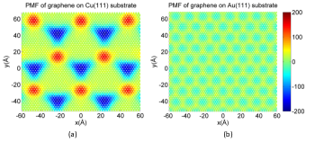
Figure 9: (Color online) PMF distributions of graphene on perfect (a) Cu (111) substrate and (b) Au (111) substrate without apertures nor gas pressure. The superlattice structure arises naturally from the need of the system to release strain buildup because of the mismatch in the lattice parameters of graphene and the underlying substrate. The PMF scale is in units of Tesla.

To reveal the PMF that is induced by the substrate alone, we show in Fig. 9 a side-by-side comparison of the PMFs that result when graphene is let to relax on Au (111) and Cu (111), respectively. The plotted data were obtained from energy minimization without pressure or aperture to show the intrinsic effect of the two substrates. Several interesting features emerge from these results, the first of which being the spontaneous development of a superlattice structure with a characteristic and well defined periodicity that is different in the two substrates. This Moiré pattern in the PMF is the result of a corresponding pattern in the strain field throughout the graphene sheet, which is caused by the need of the system to release strain buildup due to the mismatch in the lattice parameters of graphene and the substrate. A second important aspect is the considerable magnitude of the PMFs that can locally reach a few hundreds of Tesla just by letting graphene reach the minimum energy configuration in contact with the flat metal substrate. Another detail clearly illustrated by these two examples is the sensitivity to the details of the substrate interaction: the substrate-induced PMF on Cu can be many times larger than that on Au, and the Moiré period is also different. These super-periodicities are expected to perturb the intrinsic electronic structure of flat graphene whose electrons now feel the influence of this additional periodic potential. That leads, for example, to the appearance of band gaps at the edges of the folded Brillouin zone. Such effects are currently a topic of interest in the context of transport and spectroscopic properties of graphene deposited on boron nitride, where this type of epitaxial strain is conjectured to play a crucial role in determining the metallic or insulator character Woods et al. (2014); San-Jose et al. (2014); Neek-Amal and Peeters (2014); Jung et al. (2014).

Since Fig. 9 reveals a strong graphene-substrate interaction, it is not surprising that the PMF patterns in Fig. 8 are still strongly dominated by the substrate-induced PMF. Unlike the cases discussed in Fig. 4, a significant structure remains in the PMF distribution outside the hole region due to the tendency of the lattice to relax towards the characteristic Moiré periodicity of Fig. 9(a) when in contact with a flat portion of substrate. In contrast, Au (111) has a larger lattice spacing and generates considerably less epitaxial strain in the graphene film, implying comparatively weaker PMFs. It is then natural that in the presence of the nanobubbles the geometry of the aperture dominates the final PMF distribution over the entire system when pressed against Au (111) (Fig. 6), whereas for Cu (111) the epitaxial contribution is the one that dominates (Fig. 8).

VI Bending effects

The large deflection-to-linear dimension ratio in the inflated graphene bubbles analyzed so far calls for an analysis of the relative importance of the contribution to the PMF from bending in comparison with that from the local stretching of the distance between carbon atoms.

When full account of stretching and bending is taken by replacing the hopping (4) in the definition of the vector potential $\mathbf{A}$ given in Eq. (7) the resulting PMF can have considerably higher magnitudes, as was already seen in Fig. 2(f). To isolate the effect of bending alone one can split the full hopping (4) in two contributions, $t_{ij}=t_{ij}^{(xy)}+t_{ij}^{(c)}$, where the “in plane” stretching term is simply

$$-t_{ij}^{(xy)}=V_{pp\pi}(d).$$ (10)

Since the gauge field $\mathbf{A}$ is a linear function of the hopping (7), it can be likewise split into the respective stretching and bending contributions so that $\mathbf{A}=\mathbf{A}^{\!(xy)}+\mathbf{A}^{\!(c)}$. When the PMF associated with $\mathbf{A}^{\!(c)}$ is thus calculated for the circular bubble of Fig. 2 we obtain the result shown in Fig. 10(a). As was already seen when comparing the different PMF curves in Fig. 3, the effect of the curvature at the edges is quite remarkable and overwhelmingly dominant in that region.

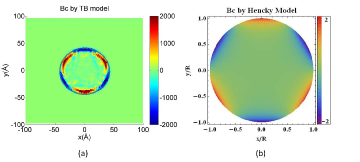
Figure 10: (Color online) Density plot of the bending contribution to the pseudomagnetic field, $B^{(c)}$, for a circular graphene bubble with radius of 4 nm and a deflection of $\sim 1$ nm calculated by the TB method (a) and Hencky’s model (b). The axes in (b) are scaled in units of the circle radius. The PMF scale is in units of Tesla. The edge of the substrate aperture used in the MD simulation is outlined (gray line) for reference.

Figure 11: (Color online) Ratio of the maximum PMF induced by bending and stretching ($B_{c}/B_{xy}$) for circular graphene bubbles as a function of the graphene radius $R$, according to Hencky’s solution.

More importantly, this fact could have been underappreciated if the stretching and bending contributions had been extracted only on the basis of an analytical solution of the elastic problem such as Hencky’s model. To be definite in this regard let us consider the magnitude of the contribution to the PMF that comes from bending in the continuum limit. If a gradient expansion of the full hopping (4) is performed, the vector potential (7) can be expressed in terms of quadratic combinations of the second derivatives of the deflection $h(x,y)$ Pereira et al. (2010a). For example, the term $V_{pp\pi}(d)\,\mathbf{n}_{i}\cdot\mathbf{n}_{j}$ in (4) leads to

$$A_{x}^{\!(c)} =-\frac{3a^{2}V_{pp\pi}^{0}}{8qv_{F}}\left[\Bigl{(}\frac{\partial^{2}{h}}{\partial{y^{2}}}\Bigr{)}^{\!\!2}-\Bigl{(}\frac{\partial^{2}{h}}{\partial{x^{2}}}\Bigr{)}^{\!\!2}\right]\!\!,$$ (11a)

$$A_{y}^{\!(c)} =-\frac{3a^{2}V_{pp\pi}^{0}}{4qv_{F}}\left[\frac{\partial^{2}{h}}{\partial{x}\partial{y}}\Bigl{(}\frac{\partial^{2}{h}}{\partial{y^{2}}}+\frac{\partial^{2}{h}}{\partial{x^{2}}}\Bigr{)}\right]\!\!.$$ (11b)

This particular contribution was previously discussed by Kim and Castro Neto (2008) and, since all the bending terms have the same scaling $\sim a^{2}h^{2}/R^{4}$, where $h$ and $R$ are the characteristic height and radius, respectively, consideration of this one alone suffices for our purpose of establishing the magnitude of the bending terms in comparison with the stretching one. Replacing the deflection $h(x,y)$ provided by Hencky’s solution in Eqs. (11) leads to the result shown in Fig. 10(b); it is clear that the maximum $B_{c}$ so obtained at the edges is much smaller than the one derived from the atomistic simulation with the full hopping. It is not surprising that the PMF coming from bending at the level of Hencky’s model is so small. A simple scaling analysis of the vector potentials in the continuum limit shows that, from Eq. (8), $\mathbf{A}_{xy}$ scales with strain as $\mathbf{A}_{xy}\sim\epsilon$ and strain itself scales with deflection as $\epsilon\sim(h/R)^{2}$ for a characteristic linear dimension $R$ of the bubble. On the other hand, from (11) $\mathbf{A}_{c}$ scales like $\mathbf{A}_{c}\sim(ah)^{2}/R^{4}$. Therefore, the ratio $B_{c}/B_{xy}$ will scale as $\sim(a/R)^{2}$. Since the bubble under analysis has $a/R\approx 0.04$ the bending contribution is indeed expected to be much smaller than the stretching one. We can even be more quantitative and extract the maximum values of $B_{c}$ and $B_{xy}$ from Hencky’s solution and compare their relative magnitudes as a function of circle radius, as shown in Fig. 11. Hencky’s solution predicts that only when the radius of the circular bubble decreases below about 1 nm does the contribution of the curvature-induced pseudomagnetic field become of the same order as that due to in-plane stretching. This situation is equivalent to the need to account for the curvature and orbital re-hybridization when describing the electronic structure of carbon nanotubes with diameters below length scales of this same magnitude at the tight-binding level Blase et al. (1994); Kane and Mele (1997); the neglect of these effects in the nanotube case leads to incorrect estimation of the band gaps and even of their metallic or insulating character.

The problem with these considerations is that they fail to anticipate the large effect at the edges, particularly the scaling analysis which tells us only about the relative magnitude of bending vs stretching in the central region. But, because we are inflating graphene under very high pressures in order to achieve deflections of the order of 1 nm, a sharp bend results at the edge of the substrate aperture through which graphene can bulge outwards; it is this curvature effect that dominates the PMF plot in Fig. 10, not the overall curvature of the bubble on the large scale. Hencky’s solution cannot capture this since it is built assuming zero radial bending moment at the edge Fichter (1997). Moreover, since this happens within a distance of the order of the lattice constant itself, the details of the displacements at the atomistic level including non-linearity and softening at large strains and curvatures become crucial. This further highlights the importance of accurate atomistic descriptions of the deformation fields in small structures such as the sub-5 nm graphene bubbles we have considered in this paper, and which have been shown experimentally to lead to significant pseudomagnetic fields Levy et al. (2010); Lu et al. (2012); at this level models based on continuum elasticity theory can become increasingly limited for accurate quantitative predictions and should be applied with caution.

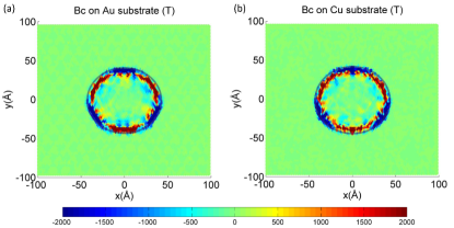
Figure 12: (Color online) Density plot of the bending contribution to the pseudomagnetic field, $B^{(c)}$, for a graphene bubble deflected to $\sim 1$ nm upon pressuring through a circular aperture of radius 4 nm in a Au (a) and a Cu (b) substrate. The PMF scale is in units of Tesla. The edge of the substrate apertures used in the MD simulations is outlined (gray line) for reference.

Finally, when realistic substrate conditions are considered, one can see that the slippage effects contribute very differently for the PMFs arising from stretching and from bending. A general feature of the PMF distribution obtained with realistic Au and Cu substrates is its smaller overall magnitude in comparison with the artificially clamped nanobubbles. This is easy to understand because the ability to slide in contact with the substrate allows graphene to stretch not only in the bubble region, but essentially everywhere, thereby reducing the strain concentration around the edge of the aperture; and with smaller strain gradients one gets smaller PMFs. The bending effects, on the other hand, are not expected to be much affected by the sliding, especially when comparing nanobubbles with the same amount of vertical deflection, because the sharpness of the bend at the edge of the aperture is constrained mostly by the geometry alone. Direct inspection of the contribution to the PMF arising from curvature in the Au and Cu substrates directly confirms this intuitive expectation, as shown in Fig. 12. Just as in the clamped case where graphene is pinned to the substrate and cannot slide, the PMF associated with bending is seen to dominate the field distribution, with magnitudes similar to the registered in Fig. 10, and much larger than the PMF in the center of the bubble or the substrate region (cf. Figs. 6 and 8). This not only shows how crucial the PMF associated with bending can be in certain approaches to generate graphene nanobubbles, but also that it is an effect largely insensitive to the details of the substrate.

VII Discussion and conclusions

We have evaluated the strain-induced pseudomagnetic fields in pressure-inflated graphene nanobubbles of different geometries and on different substrates whose configurations under pressure were obtained by classical MD simulations. The geometry of the nanobubbles is established by an aperture of prescribed shape in the substrate against which a graphene monolayer is pressed under gas pressure. Our results provide new insights into the nature of pseudomagnetic fields determined by the interplay of the bubble shape and the degree of interaction with the underlying substrate. On a technical level, if bending is (or can be) neglected, we have established that an approximate displacement-based approach is adequate to obtain the strain tensor and accurate values of the pseudomagnetic fields from MD simulations when compared with a direct tight-binding approach where the modified hoppings are considered explicitly.

By comparing nanobubbles inflated in three different substrate scenarios — namely, an arguably artificial, simply clamped graphene sheet with no substrate coupling and more realistic conditions where the full interaction with Au (111) and Cu (111) substrates is included from the outset in the MD simulations — we demonstrated that the graphene-substrate interaction is an essential aspect in determining the overall distribution and magnitude of strain and the PMFs both inside and outside the aperture region. For example, sections IV and V demonstrate that graphene can adhere substantially to the substrate in atomically flat regions leading to sizable PMFs stemming only from epitaxial strain, even in the absence of any pressure or substrate patterning. This adhesion varies from substrate to substrate and, in the presence of an aperture or other substrate patterning, perturbs the final strain distribution of the nanobubble when compared with a simply clamped edge. On a more quantitative level, in the cases analyzed here where the aspect ratio of the bubbles is close to 1, the magnitude of the PMFs associated with epitaxial strain alone can easily be of the same magnitude as the PMF generated within the bubble region. For Cu this is clear in Figs. 8 and 9, and implies that the presence of the aperture is not the main factor determining the field distribution.

To better appreciate this aspect, we can inspect the averaged cross-section of the PMF provided in Fig. 15 whose the details are given in Appendix B. The key message conveyed by the data there is that under more realistic conditions describing the graphene-substrate interaction, and for the range of parameters explored here, the PMFs are no longer concentrated in and around the aperture. The section shown reveals that the PMF can be considerably higher in regions well outside the aperture than inside or near the edge. This arises because, on the one hand, the graphene-substrate interaction alone is able to generate considerable local strain gradients that beget PMFs as large as the ones that appear by forcing the inflation of graphene through the aperture [cf. Fig. 9]. On the other hand, the fact that graphene can slip into the aperture when simulated on the Au and Cu substrates softens the strain gradients in its vicinity in comparison with the artificially clamped scenario. Slippage under these realistic substrate conditions prevents strain from concentrating solely within the aperture region which, instead, spreads to distances significantly away from the aperture. This is a sensible outcome on account of the very large stretching modulus of graphene that tends to penalize stretching as much as possible. We illustrate this behavior in Fig. 13(a) that compares the magnitude of the radial displacement of circular nanobubbles. Whereas in the artificially clamped nanobubble graphene remains undisturbed (by design) outside the aperture, it is clear that in either the Au or Cu substrates the carbon atoms pertaining to the region initially outside the aperture are radially pulled everywhere towards it under pressure, as one intuitively expects. One consequence of this is the softening of strain gradients in the bubble region: slippage naturally tends to diminish the PMFs generated within and around the aperture. The other is that, obviously, the deflection at the center is increased, as shown in Fig. 13(b).

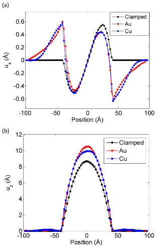
Figure 13: (Color online) The radial and vertical displacement components of graphene along the diametral section $y=0$ of three circular nanobubbles of radius 4 nm, corresponding to the three substrate conditions considered in this report. Panel (a) shows the component $u_{x}$ of the graphene in-plane displacement which corresponds, in essence, to the radial displacement because of the circular symmetry. Panel (b) shows the vertical deflection. All cases were inflated under the same pressure of $\approx 19$ kBar.

The joint effect of these two factors (slippage and adhesion to the substrate) is that forcing graphene into a nanobubble profile at the center of the system is no longer effective in concentrating the strain gradients and, consequently, the PMF is no longer more prominent there. One immediate implication of this is the fact that whether or not it is feasible to locally tailor the PMF distribution on very small (nanometer) scales depends not only on the elastic response of graphene or its loading and geometric constraints, but also on the nature of the substrate involved.

It is also clear from the above that there might exist certain substrates in which the epitaxial strain can be significant enough to, by itself, lead to visible modifications of the electronic structure of graphene, and even lead to modified transport characteristics San-Jose et al. (2014); Jung et al. (2014); Neek-Amal and Peeters (2014). Incidentally our pressure-based approach facilitates and promotes a uniform adhesion because graphene is compressed against the substrate. It would be interesting to experimentally study graphene on top of such substrates inside pressure chambers, and assess the degree of control that can be achieved over the Moire patterns and the modifications of the electronic and transport characteristics.

Another important factor to consider in estimating the magnitude and profile of the PMF generated under a given set of force distributions and geometric constraints is whether those conditions lead to strong local curvature of the graphene lattice. We analyzed this issue here by separately considering the contributions from bond bending and from stretching to the PMF in the representative case of circular nanobubbles. Our results establish that, even though the overall, large-scale curvature of the graphene sheet leads to significant corrections to the pseudomagnetic field only in ultra-small bubbles with diameter smaller than 2 nm, sharp bends arising from direct clamping or from being pressed against an edge in the substrate aperture result in much stronger PMFs locally. At the qualitative level this is naturally expected and certainly not surprising. What is surprising significant is that the bending contribution can be many times larger than its stretching counterpart, leading to a PMF distribution dominated by large values near the edges of the substrate apertures. Moreover, since this is a local geometric effect, it does not depend on the bubble size but only on the local curvature around sharp bends, and should remain in considerably larger systems. This indicates that curvature of the graphene sheet should certainly not be ignored in many situations involving out-of-plane deflection, even though the scaling analysis based on the overall profile could point otherwise.

Finally, we underline once more that the strategy to generate graphene nanobulges through gas pressure was chosen here to minimize other external forces and influences on the deflection and slippage of graphene while being able to produce deflections and aspect ratios equal to those reported in recent experiments that explore the local electronic properties of these structures. But the conclusions and implications discussed above certainly carry to various other means of achieving such or similar nanobubbles and have, therefore, a wide reach and wide import beyond graphene pressurized through apertures.

Note added. Recently, we became aware of a recent proposal to connect structure and electronic properties of two-dimensional crystals based on concepts from discrete geometry that allows yet another efficient alternative to obtain the strain and PMF at discrete lattice points without the need, for example, to perform numerical derivatives upon the displacement fields or vector potentials extracted from the MD data Barraza-Lopez et al. (2013); Pacheco Sanjuan et al. (2014).

Appendix A Angular averaging of the PMF

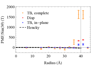
Figure 14: (Color online) Angular-averaged amplitude of the PMF for the same cases presented in Fig. 2 in the form of density plots. The horizontal axis represents the distance from the center of a pressurized circular graphene nanobubble with clamped boundary conditions. The data contained here is the same shown in Fig. 3(a), except that here the (orange) data corresponding to the PMF obtained from the full hopping perturbation [Eq. (4)] is included for comparison as well. The bending effects are clearly dominant around the edge/clamping region. Away from the edge, and inside, the three numerical curves follow Hencky’s model.

Fig. 14 below shows the radial dependence of the averaged PMF amplitude close to the edge of the circular aperture for the clamped circular case discussed in section III (Fig. 2). In Fig. 3 we plot the amplitude of the PMF at the edge of the circular aperture in the substrate for various inflation pressures with clamped graphene. In Fig. 5(b) we show the average amplitude of the PMF at different distances from the center.

In all these cases, the data shown reflect the PMF amplitude averaged over the azimuthal direction. To extract the average PMF at a given radius, the 2D distribution of the field is divided into a sequence of radial and azimuthal bins (annular sectors). For each radial annulus there are 20 bins, each with a 18 degree width. The width of the radial annulus is chosen such that at least 10 atoms lie in each bin (this is why there are fewer data points near the center of the bubble). The average and standard deviations of the PMF in each bin correspond to the value and error bar of that bin. For example, each point in Fig. 5(c) corresponds to this average PMF for a given bin. Afterwards, for each radial annulus the data is fit to the expected $\sin(3\theta)$ dependence. The amplitude of the best fit is plotted as a point [e.g., as in Fig. 14] and the fitting error provides the error bar.

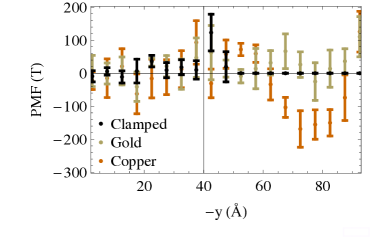
Figure 15: (Color online) The PMF of graphene pressurized through equally sized circular apertures along a vertical section extending from the center of the aperture to the bottom of the simulation cell. The vertical line at $\sim 40$ Å marks the radius of the apertures. See the text in Appendix B for more details.

Appendix B Sectional plot of PMFs for circular apertures

To better illustrate the magnitude of the PMF in the vicinity of apertures simulated under realistic substrate conditions, we present here a sectional view of the field for the representative cases of the circular apertures simulated in the artificially clamped, Au, and Cu scenarios explored in the main text. Fig. 15 shows the PMF of graphene pressurized through circular apertures of the same size sampled along a vertical section extending from the center of the aperture to the bottom of the simulation cell. The sections are taken from the corresponding data shown in Figs. 4(a), 6(a), and 8(a) by sampling the PMF along a vertical direction and performing averages within square bins of 25 Ų. The averaging is done to account for local fluctuations in the PMF and the standard deviation in each bin is used to draw the error bars. The traces in Fig. 15 are analogous to the ones in Figs. 14 or 3(a), with the exception that there is no angular averaging here because the substrate interaction breaks the rotational symmetry [cf., for example, the region outside the aperture in Fig. 8]; consequently the error bars are higher here than in the artificially clamped cases.

Appendix C Comparison of PMFs from displacement and full TB approaches

As described in the main text, the displacement approach to obtain the pseudomagnetic fields throughout the graphene sheet consists in directly employing Eq. (8), where the components of the strain tensor are extracted numerically from the MD-relaxed atomic positions. Apart from contributions beyond linear order in strain, this should be equivalent to computing the vector potential $\mathbf{A}(\mathbf{R})$ directly from the definitions (7) and (4), but neglecting the bending effects in the hopping. This amounts to considering $-t_{ij}=V_{pp\pi}(d)$.

For completeness, and to show that the two approaches lead to the same results in practice, we present in Fig. 16 the PMF distribution computed by the displacement approach for the same systems analyzed in Fig. 4. The agreement is very satisfactory and shows that the displacement and tight-binding methods are equivalent if curvature can be neglected.

Appendix D Comparison of Displacement and Stress Approaches

The final (inflated bubble) configuration gives us the basic ingredients needed to calculate the strain, i.e., the deformed atomic positions. Here we present further details on the displacement and stress approaches we investigated for calculating the strain. In the end, the stress approach revealed itself inadequate to accurately capture the local strain in the graphene lattice.

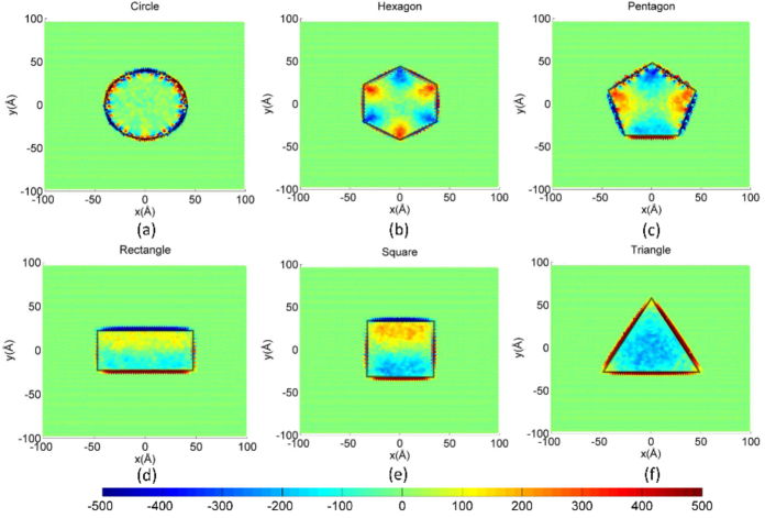
Figure 16: (Color online) PMF distribution for the same systems analyzed in Fig. 4, but here the field is computed by the displacement approach discussed in the main text. The PMF scale is in units of Tesla. The edge of the substrate apertures used in the MD simulations is outlined (gray line) for reference.

D.1 Displacement Approach

We begin with the continuum definition for strain Zimmerman et al. (2009), which is written as

$$\epsilon_{ij}=\frac{1}{2}\left(\frac{\partial{u_{i}}}{\partial{X_{j}}}+\frac{\partial{u_{j}}}{\partial{X_{i}}}\right)+\frac{1}{2}\frac{\partial{u_{k}}}{\partial{X_{i}}}\frac{\partial{u_{k}}}{\partial{X_{j}}},$$ (12)

where $\epsilon_{ij}$ are the components of the strain, $u$ is the displacement, and $X$ denotes the position of a point in the reference configuration. To compute the displacement field that is needed to evaluate the strain in Eq. 12, we first exploit the geometry of the graphene lattice by meshing it using tetrahedral finite elements Hughes (1987), where each finite element is comprised of four atoms. To remove spurious rigid body translation and rotation modes, we choose the deformed position of the atom of interest (atom 0) to be the reference position, i.e., $\mathbf{r}_{0}=\mathbf{R}_{0}$.

By subtracting the original position of each neighboring atom from its deformed position, we obtain the displacement vectors of the three nearest neighbors: $\mathbf{u_{01}}=(u_{01x},u_{01y},u_{01z})$, $\mathbf{u_{02}}=(u_{02x},u_{02y},u_{02z})$, $\mathbf{u_{03}}=(u_{03x},u_{03y},u_{03z})$.

We use the linear interpolation property of the four-node tetrahedral element to denote the displacement field $\mathbf{U}(x,y,z)=(U_{x},U_{y},U_{z})$ inside the tetrahedral element as: $U_{x}=a_{1}x+a_{2}y+a_{3}z$, $U_{y}=a_{4}x+a_{5}y+a_{6}z$, $U_{z}=a_{7}x+a_{8}y+a_{9}z$, where $a_{1}$ to $a_{9}$ are unknown constants for each tetrahedral element. Inserting the positions ($\mathbf{r_{1}}=(x_{1},y_{1},z_{1})$, $\mathbf{r_{2}}=(x_{2},y_{2},z_{2})$, $\mathbf{r_{3}}=(x_{3},y_{3},z_{3})$) and the corresponding displacements ($\mathbf{u_{01}}$,$\mathbf{u_{02}}$,$\mathbf{u_{03}}$) of the three neighboring atoms, we can solve $a_{1}$ to $a_{9}$ in terms of $\mathbf{r_{1}}$, $\mathbf{r_{2}}$, $\mathbf{r_{3}}$ and $\mathbf{u_{01}}$, $\mathbf{u_{02}}$ and $\mathbf{u_{03}}$, thus obtaining all coefficients of $\mathbf{U}(x,y,z)$. If we rearrange $\mathbf{U}(x,y,z)$ to express it in terms of $\mathbf{u_{01}}$,$\mathbf{u_{02}}$ and $\mathbf{u_{03}}$, we obtain the following equation:

$$\left[\begin{matrix}U_{x}\\ U_{y}\\ U_{z}\\ \end{matrix}\right]\!\!=\!\!\left[\begin{matrix}N_{1}&0&0&N_{2}&0&0&N_{3}&0&0\\ 0&N_{1}&0&0&N_{2}&0&0&N_{3}&0\\ 0&0&N_{1}&0&0&N_{2}&0&0&N_{3}\\ \end{matrix}\right]\!\!\left[\begin{matrix}u_{01x}\\ u_{01y}\\ u_{01z}\\ u_{02x}\\ u_{02y}\\ u_{02z}\\ u_{03x}\\ u_{03y}\\ u_{03z}\\ \end{matrix}\right]\!\!,$$ (13)

where $N_{i}=N_{i}(x,y,z),i=1,2,3$ are the finite element shape functions. For simplicity, we can rewrite Eq. (13) as:

$$\mathbf{U}=\mathbf{N}\bm{\cdot}\mathbf{u_{N}},$$ (14)

where $\mathbf{u_{N}}=[\mathbf{u_{01}},\mathbf{u_{02}},\mathbf{u_{03}}]^{T}$ is the displacement field of the three neighbor atoms.

After we obtain the displacement field $\mathbf{U}$, the strain can be derived by differentiating Eq. (14) following the continuum strain as defined in Eq. (12) to give

$$\mathbf{\epsilon}=\mathbf{T}\bm{\cdot}\mathbf{u_{N}},$$ (15)

where $\mathbf{T}=\frac{\partial\mathbf{N}}{\partial\mathbf{x}}$ is constant inside each tetrahedral element. Once the strains for each atom are determined, the vector gauge field $\mathbf{A}$ is straightforward to compute. However, to get the pseudomagnetic field, $B=\partial_{x}A_{y}-\partial_{y}A_{x}$, another derivative is needed, calculated in a similar fashion as the strain is calculated from the displacement field. Thus, the displacement approach involves two numerical derivatives, but no approximation is made about material properties.

Figure 17: (Color online) $\epsilon_{xx}$ distribution by displacement approach for uniaxial stretching case with 10 % strain.

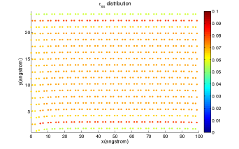
Figure 18: (Color online) $\epsilon_{xx}$ distribution by stress approach for uniaxial stretching case with 10 % strain.

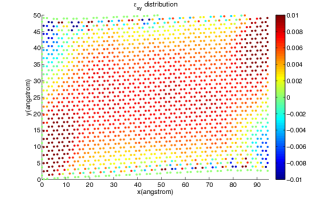
Figure 19: (Color online) $\epsilon_{xy}$ distribution by displacement approach for simple shear case with 1 % strain.

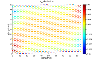
Figure 20: (Color online) $\epsilon_{xy}$ distribution by stress approach for simple shear case with 1 % strain.

D.2 Stress Approach

In MD simulations, the atomic virial stress can be extracted on a per-atom basis. In the present work, the virial stress as calculated from LAMMPS Thompson et al. (2009) was obtained for the final (inflated) graphene bubble configuration. These stresses were then related to the strain via a linear constitutive relationship, as was done recently by Klimov et al. (2012). In the current work, we utilized a plane stress model for graphene, where the in-plane strains are written as $\epsilon_{xx}=\frac{1}{E}(\sigma_{xx}-\mu\sigma_{yy})$, $\epsilon_{yy}=\frac{1}{E}(\sigma_{yy}-\mu\sigma_{xx})$, $\epsilon_{xy}=\frac{\sigma_{xy}}{G}$. The material properties of graphene are chosen as $E$ = 1 TPa Huang et al. (2006), $G$ = 0.47 TPa Min and Aluru (2011) and $\mu$ = 0.165 Blakslee et al. (1970), where $E$ is the Young’s modulus, $G$ the shear modulus, and $\mu$ Poisson’s ratio. It is important to note that, because a linear stress-strain relationship is assumed, the resulting strain is generally underestimated, particularly at large deformations due to the well-known nonlinear stress-strain response of graphene Lee et al. (2008).

Both potential and kinetic parts were taken into account for virial stress calculation. We note that the virial stress calculated in LAMMPS is in units of “Pressure$\,\cdot\,$Volume”, and thus we used the standard value of 3.42 Å as the effective thickness of single layer graphene Huang et al. (2006) to calculate the stress. A plane stress constitutive model was utilized to calculate the strain via

$$\left[\begin{matrix}\epsilon_{xx}\\ \epsilon_{yy}\\ \epsilon_{xy}\\ \end{matrix}\right]=\left[\begin{matrix}\frac{1}{E}&-\frac{\mu}{E}&0\\ -\frac{\mu}{E}&\frac{1}{E}&0\\ 0&0&\frac{1}{2G}\\ \end{matrix}\right]\cdot\left[\begin{matrix}\sigma_{xx}\\ \sigma_{yy}\\ \sigma_{xy}\\ \end{matrix}\right],$$ (16)

where the constitutive parameters are given in the main text of the manuscript.

After the strain is obtained, the same method as in the displacement approach was used to calculate the vector gauge field $\mathbf{A}$ and the pseudomagnetic field $B$. The stress approach avoids one numerical differentiation but a constitutive approximation is involved, i.e., that the stress-strain response for graphene is always linear.

D.3 Benchmark Examples

We compare the displacement and stress approaches via two simple benchmark examples, those of uniaxial stretching and simple shear. For the uniaxial stretching case, $\epsilon_{xx}\approx 10\,\%$ strain was applied along the x-direction. The loading was done by applying a ramp displacement that went from zero in the middle of simulation box to a maximum value at the +x and -x edges of the graphene monolayers.

For the simple shear case, $\epsilon_{xy}\approx 1\,\%$ shear strain was applied by fixing the -x edge and displacing the +x edge in the y-direction. Both the uniaxial stretching and simple shear simulations were performed via classical MD simulations using the open source LAMMPS Lammps (2012) code with the AIREBO potential Stuart et al. (2000). The result for the uniaxial stretching is shown in Figs. 20 and Fig. 20, while the simple shear is shown in Figs. 20 and Fig. 20. The superior performance of the displacement approach is seen in both cases. Specifically, because a linear stress-strain relationship is assumed in the stress approach as shown in Eq. (16), the resulting strain is generally underestimated, particularly at large deformations due to the well-known nonlinear stress-strain response of graphene Lee et al. (2008).

Once the strain distribution is determined from the MD simulations the PMF, $B$, can be directly evaluated from the definitions above. However, if the strain tensor is calculated within the deformation approach, a second numerical derivative is needed to get $B$, which is likely to introduce a certain degree of error. Nevertheless we found the errors to be of acceptable magnitude.

Compared with the displacement approach, the stress approach avoids one numerical differentiation, but a constitutive approximation is involved. To compare the accuracy of the displacement and stress approaches, we calculated the PMF distribution in a circular bubble (for which an analytic solution is available and detailed analysis was recently performed Kim et al. (2011)) by obtaining the strain via three different methods, as illustrated in Fig. 2: an analytic continuum mechanics model, i.e., the Hencky solution Fichter (1997) (b), the MD-based displacement approach (c), and the MD-based stress approach (d). In the MD simulations we used 100 snapshots over 5 ps during thermal equilibrium to determine the average final position and stress for the inflated bubbles. For all three models, the radius of the circular hole was 3 nm, while the final deflection was about 1 nm.

As Fig. 2 demonstrates, the PMFs generated from the MD-based displacement approach are in good agreement with those that follow from Hencky’s analytic solution, and also with previously reported values for a circular bubble Kim et al. (2011). In contrast, the stress approach fails to yield reasonable results for this loading situation, even at the qualitative level.

References

- Novoselov et al. (2005) K. S. Novoselov, A. K. Geim, S. V. Morozov, D. Jiang, M. I. Katsnelson, I. V. Grigorieva, S. V. Dubonos, and A. A. Firsov, Nature 438, 197 (2005).
- Geim and Novoselov (2007) A. K. Geim and K. S. Novoselov, Nature Materials 6, 183 (2007).
- Castro Neto et al. (2009) A. H. Castro Neto, F. Guinea, N. M. R. Peres, K. S. Novoselov, and A. K. Geim, Reviews of Modern Physics 81, 109 (2009).
- Han et al. (2007) M. Y. Han, B. Ozyilmaz, Y. Zhang, and P. Kim, Physical Review Letters 98, 206805 (2007).
- Seol et al. (2010) J. H. Seol, I. Jo, A. L. Moore, L. Lindsay, Z. H. Aitken, M. T. Pettes, X. Li, Z. Yao, R. Huang, D. Broido, et al., Science 328, 213 (2010).
- Guinea et al. (2010a) F. Guinea, M. I. Katsnelson, and A. K. Geim, Nature Physics 6, 30 (2010a).
- Qi et al. (2013) Z. Qi, D. A. Bahamon, V. M. Pereira, H. S. Park, D. K. Campbell, and A. H. Castro Neto, Nano Letters 13, 2692 (2013).
- Tomori et al. (2011) H. Tomori, A. Kanda, H. Goto, Y. Ootuka, K. Tsukagoshi, S. Moriyama, E. Watanabe, and D. Tsuya, Applied Physics Express 4, 3 (2011).
- Guinea et al. (2010b) F. Guinea, A. K. Geim, M. I. Katsnelson, and K. S. Novoselov, Physical Review B 81, 035408 (2010b).
- Pereira and Castro Neto (2009) V. M. Pereira and A. H. Castro Neto, Physical Review Letters 103, 046801 (2009).
- Guinea and Low (2010) F. Guinea and T. Low, Philosophical Transactions of the Royal Society a-Mathematical Physical and Engineering Sciences 368, 5391 (2010).
- Guinea et al. (2008) F. Guinea, B. Horovitz, and P. Le Doussal, Physical Review B 77, 205421 (2008).
- Abedpour et al. (2011) N. Abedpour, R. Asgari, and F. Guinea, Physical Review B 84, 115437 (2011).
- Kim et al. (2011) K.-J. Kim, Y. M. Blanter, and K.-H. Ahn, Physical Review B 84, 081401 (2011).
- Yeh et al. (2011) N. C. Yeh, M. L. Teague, S. Yeom, B. L. Standley, R. T. P. Wu, D. A. Boyd, and M. W. Bockrath, Surface Science 605, 1649 (2011).
- Yang (2011) H. T. Yang, Journal of Physics-Condensed Matter 23 (2011).
- Kitt et al. (2012) A. L. Kitt, V. M. Pereira, A. K. Swan, and B. B. Goldberg, Physical Review B 85, 115432 (2012).
- Kitt et al. (2013a) A. L. Kitt, V. M. Pereira, A. K. Swan, and B. B. Goldberg, Physical Review B 87, 159909(E) (2013a).
- Yue et al. (2012) K. Yue, W. Gao, R. Huang, and K. M. Liechti, Journal of Applied Physics 112, 083512 (2012).
- Pereira et al. (2010a) V. M. Pereira, A. H. Castro Neto, H. Y. Liang, and L. Mahadevan, Physical Review Letters 105, 156603 (2010a).
- Abanin and Pesin (2012) D. A. Abanin and D. A. Pesin, Physical Review Letters 109, 066802 (2012).
- Wang et al. (2011) Z. F. Wang, Y. Zhang, and F. Liu, Physical Review B 83, 041403 (2011).
- Pereira et al. (2009) V. M. Pereira, A. H. Castro Neto, and N. M. R. Peres, Physical Review B 80, 045401 (2009).
- Ni et al. (2009) Z. H. Ni, T. Yu, Y. H. Lu, Y. Y. Wang, Y. P. Feng, and Z. X. Shen, ACS Nano 3, 483 (2009).
- Farjam and Rafii-Tabar (2009) M. Farjam and H. Rafii-Tabar, Physical Review B 80, 167401 (2009).
- Choi et al. (2010) S.-M. Choi, S.-H. Jhi, and Y.-W. Son, Physical Review B 81, 081407(R)+ (2010).
- Kane and Mele (1997) C. L. Kane and E. J. Mele, Physical Review Letters 78, 1932 (1997).
- Suzuura and Ando (2002) H. Suzuura and T. Ando, Physical Review B 65, 235412 (2002).
- Pereira et al. (2010b) V. M. Pereira, R. M. Ribeiro, N. M. R. Peres, and A. H. Castro Neto, Eur. Phys. Lett. 92, 67001 (2010b).
- Gong et al. (2010) L. Gong, I. A. Kinloch, R. J. Young, I. Riaz, R. Jalil, and K. S. Novoselov, Adv. Mater. 22, 2694 (2010).
- Levy et al. (2010) N. Levy, S. A. Burke, K. L. Meaker, M. Panlasigui, A. Zettl, F. Guinea, A. H. Castro Neto, and M. F. Crommie, Science 329, 544 (2010).
- Lu et al. (2012) J. Lu, A. H. Castro Neto, and K. P. Loh, Nature communications 3, 823 (2012).
- Neek-Amal and Peeters (2012a) M. Neek-Amal and F. M. Peeters, Physical Review B 85, 195446 (2012a).
- Neek-Amal et al. (2012) M. Neek-Amal, L. Covaci, and F. M. Peeters, Physical Review B 86, 041405 (2012).
- Humphrey et al. (1996) W. Humphrey, A. Dalke, and K. Schulten, Journal of Molecular Graphics 14, 33 (1996).
- Lammps (2012) Lammps, http://lammps.sandia.gov (2012).
- Plimpton (1995) S. Plimpton, Journal of Computational Physics 117, 1 (1995).
- Stuart et al. (2000) S. J. Stuart, A. B. Tutein, and J. A. Harrison, Journal of Chemical Physics 112, 6472 (2000).
- Zhao and Aluru (2010) H. Zhao and N. R. Aluru, Journal of Applied Physics 108, 064321 (2010).
- Qi et al. (2010) Z. Qi, F. Zhao, X. Zhou, Z. Sun, H. S. Park, and H. Wu, Nanotechnology 21, 265702 (2010).
- Neek-Amal and Peeters (2012b) M. Neek-Amal and F. M. Peeters, Physical Review B 85, 195445 (2012b).
- Hoover (1985) W. G. Hoover, Physical Review A 31, 1695 (1985).
- Nair et al. (2012) R. R. Nair, H. A. Wu, P. N. Jayaram, I. V. Grigorieva, and A. K. Geim, Science 335, 442 (2012).
- Bunch et al. (2008) J. S. Bunch, S. S. Verbridge, J. S. Alden, A. M. van der Zande, J. M. Parpia, H. G. Craighead, and P. L. McEuen, Nano Letters 8, 2458 (2008).
- Koenig et al. (2011) S. P. Koenig, N. G. Boddeti, M. L. Dunn, and J. S. Bunch, Nature Nanotechnology 6, 543 (2011).
- Klimov et al. (2012) N. N. Klimov, S. Jung, S. Z. Zhu, T. Li, C. A. Wright, S. D. Solares, D. B. Newell, N. B. Zhitenev, and J. A. Stroscio, Science 336, 1557 (2012).
- Hughes (1987) T. J. R. Hughes, The Finite Element Method: Linear Static and Dynamic Finite Element Analysis (Prentice-Hall, 1987).
- Isacsson et al. (2008) A. Isacsson, L. M. Jonsson, J. M. Kinaret, and M. Jonson, Physical Review B 77, 035423 (2008).
- Hansson and Stafström (2003) A. Hansson and S. Stafström, Physical Review B 67, 075406 (2003).
- de Juan et al. (2013) F. de Juan, J. L. Mañes, and M. A. H. Vozmediano, Physical Review B 87, 165131 (2013).
- Sloan et al. (2013) J. V. Sloan, A. Sanjuan, Z. Wang, C. Horvath, and S. Barraza-Lopez, Physical Review B 87, 155436 (2013).
- Oliva-Leyva and Naumis (2013) M. Oliva-Leyva and G. G. Naumis, Physical Review B 88, 085430 (2013).
- Wang et al. (2013) P. Wang, W. Gao, Z. Cao, K. M. Liechti, and R. Huang, Journal of Applied Mechanics 80, 040905 (2013).
- Fichter (1997) W. B. Fichter, Tech. Rep. 3658, NASA Langley Research Center (1997).
- Wei et al. (2013) Y. Wei, B. Wang, J. Wu, R. Yang, and M. L. Dunn, Nano Letters 13, 26 (2013).
- Lee et al. (2008) C. Lee, X. Wei, J. W. Kysar, and J. Hone, Science 321, 385 (2008).
- Jun et al. (2011) S. Jun, T. Tashi, and H. S. Park, Journal of Nanomaterials 2011, 380286 (2011).
- De Martino et al. (2007) A. De Martino, L. Dell’Anna, and R. Egger, Physical Review Letters 98, 066802 (2007).
- Masir et al. (2009) M. R. Masir, P. Vasilopoulos, and F. M. Peeters, New J. Phys. 11, 095009 (2009).
- Lim et al. (2012) C. H. Y. X. Lim, A. Sorkin, Q. Bao, A. Li, K. Zhang, M. Nesladek, and K. P. Loh, Nature Communications 4, 1556 (2012).
- Kitt et al. (2013b) A. Kitt, Z. Qi, S. Rémi, H. S. Park, A. K. Swan, and B. Goldberg, Nano Letters 13, 2605 (2013b).
- Piana and Bilic (2006) S. Piana and A. Bilic, Journal of Physical Chemistry B 110, 23467 (2006).
- Tuzun et al. (1996) R. E. Tuzun, D. W. Noid, B. G. Sumpter, and R. C. Merkle, Nanotechnology 7, 241 (1996).
- Rytkönen et al. (1998) A. Rytkönen, S. Valkealahti, and M. Manninen, Journal of Chemical Physics 108, 5826 (1998).
- He et al. (2012) R. He, L. Zhao, N. Petrone, K. S. Kim, M. Roth, J. Hone, P. Kim, A. Pasupathy, and A. Pinczuk, Nano Letters 12, 2408 (2012).
- Maekawa and Itoh (1995) K. Maekawa and A. Itoh, Wear 188, 115 (1995), ISSN 0043-1648.
- Woods et al. (2014) C. Woods, L. Britnell, A. Eckmann, R. Ma, J. Lu, H. Guo, X. Lin, G. Yu, Y. Cao, R. Gorbachev, et al., Nature Physics 10, 451 (2014).
- San-Jose et al. (2014) P. San-Jose, A. Gutiérrez-Rubio, M. Sturla, and F. Guinea, Phys. Rev. B 90, 075428 (2014).
- Neek-Amal and Peeters (2014) M. Neek-Amal and F. M. Peeters, Applied Physics Letters 104, 041909 (2014).
- Jung et al. (2014) J. Jung, A. DaSilva, S. Adam, and A. H. MacDonald (2014), eprint arXiv:1403.0496.
- Kim and Castro Neto (2008) E. A. Kim and A. H. Castro Neto, Europhysics Letters 84 (2008).
- Blase et al. (1994) X. Blase, L. X. Benedict, E. L. Shirley, and S. G. Louie, Physical Review Letters 72, 1878 (1994).
- Barraza-Lopez et al. (2013) S. Barraza-Lopez, A. A. Pacheco Sanjuan, Z. Wang, and M. Vanević, Solid State Communications 166, 70 (2013).
- Pacheco Sanjuan et al. (2014) A. A. Pacheco Sanjuan, Z. Wang, H. P. Imani, M. Vanević, and S. Barraza-Lopez, Phys. Rev. B 89 (2014).
- Zimmerman et al. (2009) J. A. Zimmerman, D. J. Bammann, and H. J. Gao, International Journal of Solids and Structures 46, 238 (2009).
- Thompson et al. (2009) A. P. Thompson, S. J. Plimpton, and W. Mattson, Journal of Chemical Physics 131 (2009).
- Huang et al. (2006) Y. Huang, J. Wu, and K. C. Hwang, Physical Review B 74, 245413 (2006).
- Min and Aluru (2011) K. Min and N. R. Aluru, Applied Physics Letters 98, 013113 (2011).
- Blakslee et al. (1970) O. L. Blakslee, D. G. Proctor, E. J. Seldin, G. B. Spence, and T. Weng, Journal of Applied Physics 41, 3373 (1970).