Construction of invariant whiskered tori by a parameterization method. Part II: Quasi-periodic and almost periodic breathers in coupled map lattices.

Abstract.

We construct quasi-periodic and almost periodic solutions for coupled Hamiltonian systems on an infinite lattice which is translation invariant. The couplings can be long range, provided that they decay moderately fast with respect to the distance.

For the solutions we construct, most of the sites are moving in a neighborhood of a hyperbolic fixed point, but there are oscillating sites clustered around a sequence of nodes. The amplitude of these oscillations does not need to tend to zero. In particular, the almost periodic solutions do not decay at infinity.

The main result is an a-posteriori theorem. We formulate an invariance equation. Solutions of this equation are embeddings of an invariant torus on which the motion is conjugate to a rotation. We show that, if there is an approximate solution of the invariance equation that satisfies some non-degeneracy conditions, there is a true solution close by.

This does not require that the system is close to integrable, hence it can be used to validate numerical calculations or formal expansions.

The proof of this a-posteriori theorem is based on a Nash-Moser iteration, which does not use transformation theory. Simpler versions of the scheme were developed in E. Fontich, R. de la Llave,Y. Sire J. Differential. Equations. 246, 3136 (2009).

One technical tool, important for our purposes, is the use of weighted spaces that capture the idea that the maps under consideration are local interactions. Using these weighted spaces, the estimates of iterative steps are similar to those in finite dimensional spaces. In particular, the estimates are independent of the number of nodes that get excited. Using these techniques, given two breathers, we can place them apart and obtain an approximate solution, which leads to a true solution nearby. By repeating the process infinitely often, we can get solutions with infinitely many frequencies which do not tend to zero at infinity.

1. Introduction

The goal of this paper is to prove theorems on persistence of invariant tori in some lattice systems. These models describe copies of identical systems placed on the nodes of a lattice and interacting with all the other systems in the lattice. The interaction can be of infinite range, but it has to decay sufficiently fast with the distance. We will assume that the dynamics is Hamiltonian and, for simplicity, we will also assume that the dynamics is analytic. We will consider “whiskered tori”. These are invariant tori such that the motion on them is a rotation and which are as hyperbolic as possible, compatible with the fact that the motion is an irrational rotation (it is well known that the directions symplectically conjugate to the tangent of the tori have to be neutral). See Definition 3.1.

The main technical tool we will develop is a theorem of persistence of finite dimensional whiskered tori, namely Theorem 3.6 below, which has sufficiently good properties to allow us to use it recursively to construct tori with infinite frequencies.

The tori we consider in Theorem 3.6 are finite dimensional whiskered tori with some local character. The motion on the torus is a rigid rotation with a Diophantine frequency. The preservation of the symplectic structure and the rotational motion on the tori force that there are some neutral directions in the normal directions. We will assume that, except for these directions, the normal directions are hyperbolic (they expand at exponential rates either in the future or in the past). In particular, the hyperbolic spaces are infinite dimensional.

The main technique to prove Theorem 3.6 is to derive an equation that implies invariance of the torus and that the motion on it is a rotation and to develop a theory for solutions of the equation.

Given a map $F$ on a phase space ${\mathcal{M}}$ and a frequency $\omega\in{\mathbb{R}}^{l}$, it is easy to see that $K:{\mathbb{T}}^{l}\rightarrow{\mathcal{M}}$ is a parameterization of a torus with a rotation $\omega$, if and only if

(1) $$F\circ K=K\circ T_{\omega}\,,$$

where $T_{\omega}$ denotes the rotation on the torus by $\omega$. Similarly, for a vector field $X$, we seek parameterizations $K$ satisfying

(2) $$X\circ K=\partial_{\omega}K,$$

where $\partial_{\omega}$ is the derivative along the direction $\omega$.

Our main result will be Theorem 3.6, which shows that if we have an approximate solution of the invariance equation which is also not too degenerate, there is a true solution which is close to the approximate one. Theorems of this form, that validate an approximate solution, will be called a posteriori, following the language in numerical analysis.

We emphasize that Theorem 3.6 does not assume that the system is close to integrable, so that the approximate solution could be produced in any way. Of course, when the system is close to integrable, we can take as approximate solutions the solutions of the integrable system, so that we recover the standard formulations of KAM theorems for quasi-integrable systems. The approximate solutions can be produced by a variety of methods, including Lindstedt series or numerical computations. In finite dimensions, some whiskered tori are generated by resonant averaging [dlLW04, Tre94] or by homoclinic tangencies [Dua08]. In such cases, Theorem 3.6 leads to justifications of the expansions or the numerical computations. We also note that Theorem 3.6 does not assume that the system is translation invariant (it assumes only the existence of some uniform bounds).

The a posteriori approach to KAM theorem was emphasized in [Mos66b, Mos66a, Zeh75, Zeh76a, Zeh76b]. There, it was pointed out that this a posteriori approach automatically allows to deduce results for finitely differentiable systems as well as to prove smooth dependence on parameters or analyticity of perturbative series. We refer the reader to [dlL01] for a comparison of different KAM methods.

In this paper, we use the a posteriori format to construct more complicated quasi-periodic solutions by juxtaposing two simpler solutions separated by a sufficiently long distance. The a posteriori format of Theorem 3.6, allows us to control the limit of the solutions, which will be an almost periodic solution. The ability to superimpose solutions far apart is greatly facilitated by assuming translation invariance, which will be an assumption in the second part of this work. One could assume significantly less (e.g. some amount of uniformity). Nevertheless, this seems a natural assumption.

One important technical tool in this paper is the use of spaces of decay functions following [JdlL00, FdlLM11a]. These are spaces of functions whose norms quantify the effect that the motion of one particle does not affect much the motion of particles far apart. Besides that, they also enjoy certain Banach algebra properties so that the hyperbolic directions can be dealt with in the same manner than in the finite dimensional spaces.

Using spaces of decay functions, we can make quantitative the observation that, since the oscillations at one site almost do not affect those further apart, superimposing oscillations centered around sites far apart produces a very approximate solution. We will call the localized oscillating solutions “breathers”. The error in the invariance equation (measured in the sense of an appropriate space of decay functions) is arbitrarily small if the centers are placed far enough. A rather simple calculation shows that the non-degeneracy conditions deteriorate also by an arbitrarily small amount. In summary, if the frequencies of the oscillations are jointly Diophantine (even if the constant is bad), we can satisfy all the requirements of the theorem by displacing the breathers far apart. If one makes appropriate choices – placing the subsequent centers of oscillation far enough apart – we will show that the process can be repeated infinitely often and that it converges in a sense which is strong enough to justify that the limit is a solution of the system. This solution contains infinitely many frequencies.

The process of coupling the breathers does not require any smallness conditions in the coupling (it suffices to place the breathers far enough apart). On the other hand, establishing the existence of breathers by perturbing from those of the uncoupled system, does require some smallness conditions. We also require some mild smallness conditions on the perturbations to ensure that the system remains non-degenerate.

In the solutions that we construct most of the sites are near a hyperbolic equilibrium. These solutions, therefore, have an average energy close to that of the equilibrium solutions and are at the border of chaos (in particular, they are dynamically unstable). There are indications that these solutions play an important role in instability.

The results of the paper were summarized in [FdlLS09a], which perhaps can be used as a reading guide to the present paper.

We also note that, after this paper was finished, the work [BdlL14], used the results of this paper to construct the whiskers of the whiskered tori constructed in this paper in a very similar functional formulation, so that the whiskers also have decay properties.

To provide some motivation, we now mention several models found in the literature for which our method applies. These models can be described by the following formal Hamiltonian

(3) $$H(p,q)=\sum_{i\in{\mathbb{Z}}^{N}}\Big{(}\frac{1}{2}|p_{i}|^{2}+W(q_{i})\Big{)}+\sum_{k\in{\mathbb{Z}}^{N}}\ \sum_{i\in{\mathbb{Z}}^{N}}V_{k}(q_{i}-q_{i+k})$$

under some assumptions on the potentials $W$ and $V_{k}$. Here the formal Hamiltonian structure is

$$\Omega_{\infty}=\sum_{i\in{\mathbb{Z}}^{N}}dp_{i}\wedge dq_{i}.$$

Note that, even if the sum defining the Hamiltonian and the symplectic form are formal and not meant to converge, Hamilton’s equations are a well behaved system of differential equations (if the $V_{k}$ decay fast enough, e.g. if they are finite range). In fact the equations of motion are

$$\begin{split}\dot{q}_{i}&=p_{i}\\ \dot{p}_{i}&=-\nabla W(q_{i})-\sum_{k\in{\mathbb{Z}}^{N}}\Big{\{}\nabla V_{k}(q_{i}-q_{i+k})-\nabla V_{k}(q_{i-k}-q_{i})\Big{\}}.\end{split}$$

The model (3) involves a local potential $W$ for each particle and interaction potentials among pairs of particles. Of course, the interaction potentials are assumed to decay with $|k|$ fast enough. The method of proof also accommodates many body interactions. One important feature of the method is that, in some appropriate weighted spaces, the estimates we obtain are independent of the number and the position of the centers of oscillation.

If we take the lattice to be with one degree of freedom, the potential $V$ to be just nearest neighbor (i.e. $V_{k}=0$ for $|k|>1$) and set $V_{1}(s)=\frac{\gamma}{2}s^{2}$, we obtain the so called 1-D Klein-Gordon system described by the formal Hamiltonian

$$H(q,p)=\sum_{n=-\infty}^{+\infty}\Big{(}\frac{1}{2}p_{n}^{2}+W(q_{n})+\frac{\gamma}{2}(q_{n+1}-q_{n})^{2}\Big{)},$$

and whose equations of motion are

(4) $$\ddot{q}_{n}+W^{\prime}(q_{n})=\gamma(q_{n+1}+q_{n-1}-2q_{n}),\,\,\,\,\,n\in{\mathbb{Z}}.$$

We note that the method we present applies to higher dimensional lattices and higher dimensional systems. We also do not need to assume that the symplectic form is the standard one. This is convenient when the symplectic form is degenerate. Changes in the symplectic form correspond to magnetic fields [Thi97]. Note that the systems with magnetic fields are not reversible.

For a review of the physical relevance of these models we refer the reader to [FW98]. Concerning the existence proof of periodic breathers, we refer to [MA94, AGT96, AG96, AKK01]. In the latter papers, the technique is based on a variational argument whereas in [MA94], the authors use an implicit function theorem. For quasi-periodic breathers in finite – but arbitrarily large systems, we mention [BV02, GY07, GVY08, CY07b]. The paper [Yua02] proves the existence of quasi-periodic breathers in the Fermi-Pasta-Ulam lattice. In all the cases above, the breathers are normally elliptic or dissipative. Quasi-periodic and almost periodic breathers for lattices of reversible systems with dissipation are considered in [CY07a].

Remark 1.1.

There is a variety of results showing that for hyperbolic PDE’s there are no quasi-periodic solutions of finite energy [Pyk96, SW99, KK08, KK10]. Since some of the models we consider are obtained as discretizations of nonlinear wave equations, it is interesting to understand why the results above do not apply to the discretized model, even if they apply to the PDE.

The reason is that the mechanism behind the proofs in the above papers is that quasi-periodic solutions of non-linear PDE’s have to radiate and send energy to infinity.

In the models we consider, there is no radiation because most of the media is near the hyperbolic regime.

We can understand the lack of radiation in the model but representative problem

(5) $$\ddot{q}_{n}+Aq_{n}=\gamma(q_{n+1}+q_{n-1}-2q_{n}),\,\,\,\,\,n\in{\mathbb{Z}},\,\gamma>0.$$

where $A<0$. The equation (5) is a linearization of (4) near the point $q=0$, which is a maximum of the potential (or a mimimum of $W$ in the notation of (4)).

We see that if we substitute solutions of the form $q_{n}=\exp(i(\omega t+kn))$ in (5), we are lead to the dispersion relation

$$-\omega^{2}+A=\gamma(2\cos(k)-2).$$

If $|\gamma|$ is small enough, this dispersion relation does not have any real solutions for $\omega$ and the only square roots are imaginary.

In this model, near the hyperbolic fixed points the equations do not propagate waves, so that there is no radiation and the arguments excluding quasi-periodic solutions in the above papers do not apply.

However, for PDE’s, the dispersion relation would be $-\omega^{2}+A=-\gamma k^{2}$. The unboudedness of the $k^{2}$ factor makes it possible to have propagating waves no matter how small $|\gamma|$ is.

Note also that in the model in [FSW86], there is no propagation either because of the random nature of the media.

2. Basic setup and preliminaries

The main goal of this paper is to extend the method introduced in [FdlLS09a] for the study of whiskered tori to some systems on infinite dimensional manifolds. The systems we will consider consist of infinitely many finite dimensional Hamiltonian systems, each of them corresponding to a site on a lattice, subject to some coupling. We will assume that the coupling decays fast enough with respect to the distance among the sites. These are standard models in many applied fields and there is a large mathematical theory, which we cannot survey systematically (but we will make some indication of the results we use or the one closer to our goals).

An important tool for us will be appropriate function spaces for these interactions. There are many other methods to establish the existence of whiskered tori [Gra74, Zeh76a, You99]. The present method has the advantage that it depends much less on the subtle geometric properties, so that it applies easily to infinite dimensional contexts.

Since we are interested in translation invariant problems and want to produce solutions that do not go to zero at infinity, it is natural to model the functional analysis in $\ell^{\infty}$, which has some subtle points that require attention.

The goal of this section is to set up the functional analysis spaces modelled after $\ell^{\infty}$ and capturing the idea that changes in one site have very small effect in sites that are far away. We anticipate that we need two types of spaces. One family of spaces for the mappings from the infinite dimensional space to itself and another kind of spaces for the mappings from a finite dimensional torus to the infinite dimensional phase space. This corresponds to the $F$, $K$ in (1) or the $X$, $K$ in (2). The spaces we choose are patterned after the choices in [JdlL00, FdlLM11a]. Other Banach spaces of functions in lattice systems are in [Rug02, BK95]. Indeed, the choice of topologies in these infinite dimensional systems is rather subtle and arguments in ergodic theory which rely more on measure theory than on geometry find useful toplogies in which the phase space is compact.

2.1. Phase spaces

In this paper we will assume that the phase space at each node is given by an Euclidean exact symplectic manifold $(M={\mathbb{T}}^{l}\times{\mathbb{R}}^{2d-l},\Omega=d\alpha)$, where ${\mathbb{T}}={\mathbb{R}}/{\mathbb{Z}}$. We will not assume that the symplectic form is given in the standard form of action-angle variables. For some calculations we consider $\tilde{M}={\mathbb{R}}^{l}\times{\mathbb{R}}^{2d-l}$, the universal covering of $M$ or the complex extensions of the above. This is natural since the KAM method requires to consider Fourier series.

It is possible to adapt our method to the case of a non-Euclidean manifold $M$ using connectors and exponential mappings. This just requires some typographical effort. See the discussion in [FdlLS09a].

Then, the phase space of the lattice system will be a subset of

(6) $$M^{{\mathbb{Z}}^{N}}=\displaystyle{\prod_{j\in{\mathbb{Z}}^{N}}}M.$$

Since $M$ is unbounded we will take as phase space

(7) $${\mathcal{M}}=\ell^{\infty}({\mathbb{Z}}^{N},M)=\Big{\{}x\in M^{{\mathbb{Z}}^{N}}\mid\,\sup_{i\in{\mathbb{Z}}^{N}}|x_{i}|<\infty\Big{\}}$$

which is a strict subset of $M^{{\mathbb{Z}}^{N}}$. We will endow ${\mathcal{M}}$ with the distance

$$d(x,y)=\sup_{i\in{\mathbb{Z}}^{N}}d(x_{i},y_{i}),$$

where $d(x_{i},y_{i})$ is the distance on the finite dimensional manifold $M$.

When $M$ is $\mathbb{R}^{2d}$, ${\mathcal{M}}$ is a Banach space with the norm

$$\|x\|_{\infty}=\sup_{i\in{\mathbb{Z}}^{N}}|x_{i}|.$$

When $M={\mathbb{T}}^{l}\times\mathbb{R}^{2d-l}$, ${\mathcal{M}}$ is a Banach manifold modelled on $\ell^{\infty}({\mathbb{Z}}^{N})$.

Notice that because $M$ is an Euclidean space, the tangent space of $\mathcal{M}$ is trivial and can be identified with $\ell^{\infty}$. Given $x\in{\mathcal{M}}$ and $\xi\in\ell^{\infty}$, we can define $x+\xi$ by just adding the components. We see that if $\|\xi\|_{\infty}<1/2$, the mapping $\xi\to x+\xi$ is injective, so that this defines a chart in ${\mathcal{M}}$.

Remark 2.1.

The fact that we assume that the manifold has the structure $M={\mathbb{T}}^{l}\times{\mathbb{R}}^{2d-l}$ is important here since it implies that $H^{1}(M)\sim H^{1}({\mathbb{T}}^{l})$ is non-trivial. This allows us to perform the construction in Appendix C. If the manifold was such that its first de-Rham cohomology group were trivial, all the symplectic maps would be exact symplectic and the construction would not work without changes. To deal with manifolds such that $H^{1}(M)$ is trivial ($M={\mathbb{R}}^{2d}$ for instance), one can use the method developed by the authors in the finite dimensional case (see [FdlLS09a, FdlLS09b]). This consists in perturbing the invariance equation for the tori by a translation term and prove, at the end of the convergence scheme, that the geometry implies that this term is zero. The method of [FdlLS09a] allows to deal with secondary tori (i.e. tori which are contractible to tori of lower dimension) directly. The present method would require to make some preliminary changes of variables.

The choice of $\ell^{\infty}$ is dictated by the fact that we want to deal with solutions that neither grow nor decrease at $\infty$. This, however, will lead to some complications, the functional analysis in $\ell^{\infty}$ being rather delicate. On the other hand, obtaining estimates in $\ell^{\infty}$ for several of our objects will be relatively easy.

Since we are going to deal with analytic functions, one has to define what is the complex extension of the manifold ${\mathcal{M}}$. By assumption, the manifold $M$ is an Euclidean manifold, hence, it admits a complex extension $M^{\mathbb{C}}$. We define the complex extension of ${\mathcal{M}}$ as a subspace of the product of the complex extensions of $M$, i.e.

$${\mathcal{M}}^{\mathbb{C}}=\Big{\{}z\in\prod_{j\in{\mathbb{Z}}^{N}}M^{\mathbb{C}}\ \Big{|}\ \sup_{i\in{\mathbb{Z}}^{N}}|z_{i}|<\infty\Big{\}}.$$

In the following, we will be considering mostly ${\mathcal{M}}^{{\mathbb{C}}}$ but to simplify the notation we will not write the superscript ${\mathbb{C}}$, if it does not lead to confusion.

2.2. Some functional analysis in $\ell^{\infty}({\mathbb{Z}}^{N})$ and the spaces of decay functions

As emphasized in [FdlLM11a], $\ell^{\infty}({\mathbb{Z}}^{N})$ has a very complicated dual space which cannot be identified with a space of sequences since there is no Riesz-representation theorem. As a consequence, we have that the matrix elements of an operator do not characterize the operator and, relatedly, the differential of a map is not represented by its partial derivatives. The physical meaning is that one has to take into account “boundary conditions at infinity”.

For example, consider the functional ${\mathcal{T}}$ defined on the closed subspace of $\ell^{\infty}({\mathbb{Z}})$ consisting of convergent sequences by the formula

$${\mathcal{T}}(u)=\lim_{n\rightarrow+\infty}u_{n}.$$

By the Hahn-Banach theorem, ${\mathcal{T}}$ extends to $\ell^{\infty}({\mathbb{Z}})$. The extended functional ${\mathcal{T}}$ is non-trivial but we have

$$\partial_{u_{i}}{\mathcal{T}}(u)=0$$

since the limit does not depend on $u_{i}$. Of course, the functional ${\mathcal{T}}$ is linear but it is not represented by a matrix. Similar phenomena have been known in statistical mechanics for a while under the name observables at infinity.

This phenomenon can be eliminated by restricting our attention to functions whose derivative is a linear functional which is given by the matrix of partial derivatives. We will develop some technology that allows to verify this assumption rather comfortably in the cases of interest. A much more thorough treatment can be found in [FdlLM11a].

2.2.1. Weighted norms to formulate decay properties

To formulate quantitatively the approximate locality of the maps we will consider Banach spaces whose norm makes precise that changing one coordinate affects little the outcome of other coordinates far away.

We will make use of the so-called decay functions introduced in [JdlL00].

Definition 2.2.

We say that a function $\Gamma:{\mathbb{Z}}^{N}\rightarrow{\mathbb{R}}_{+}$, is a decay function when it satisfies

1. $\displaystyle{\sum_{j\in{\mathbb{Z}}^{N}}}\Gamma(j)\leq 1,$

2. $\displaystyle{\sum_{j\in{\mathbb{Z}}^{N}}}\Gamma(i-j)\Gamma(j-k)\leq\Gamma(i-k),\quad\,\,\,i,k\in{\mathbb{Z}}^{N}$.

The algebraic property $(2)$ in definition 2.2 is important since it is the one that allows us to construct Banach algebras.

The following elementary proposition is proved in detail in [JdlL00] and provides an example of a decay function.

Proposition 2.3.

Given $\alpha>N$, $\theta\geq 0$, there exists $a>0$, depending on $\alpha,\theta$, $N$ such that the function defined by

$$\Gamma(i)=\left\{\begin{array}[c]{ll}a|i|^{-\alpha}e^{-\theta|i|}&\mbox{if $\;i\neq 0$,}\\ a&\mbox{if $\;i=0$}\end{array}\right.$$

is a decay function on ${\mathbb{Z}}^{N}$.

We note, as it is easily verified in [JdlL00], that $\Gamma(i)=C\exp(-\beta|i|)$ is not a decay function for any $\beta,C>0$.

If one considers other sets $\Lambda$ in place of ${\mathbb{Z}}^{N}$, such as the Bethe lattice which also admit decay functions (see [JdlL00]), many of the results of the present paper can be adapted with little change.

Definition 2.4.

Given two decay functions $\Gamma,\Gamma^{\prime}$ we say that $\Gamma$ dominates $\Gamma^{\prime}$ and write $\Gamma^{\prime}\ll\Gamma$ when

$$\lim_{k\to\infty}\Gamma^{\prime}(k)/\Gamma(k)=0.$$

We say that a family of decay functions $\Gamma_{\beta}$, $\beta\in[0,1]$, is an ordered family when $\tilde{\beta}<\beta$ implies $\Gamma_{\tilde{\beta}}\ll\Gamma_{\beta}$.

Of course the examples in Proposition 2.3 constitute an ordered family. For some of the arguments later, in the proof of Theorem 3.11, when we are increasing the scales increasing the number of breathers, it will be useful to have a full scale so that the longer scales have a weaker decay. This is the reason why Theorem 3.11 is only stated for these functions.

Of course, the examples in Proposition 2.3 enjoy several other nice properties, for example that $\Gamma(i)$ is a decreasing function of $|i|$. We refer the reader to Appendix A where a deeper study of spaces of decay functions is performed. In the following, we just give the definitions needed to state our main results.

Remark 2.5.

Prof. L. Sadun pointed out that there is a very natural physical interpretation of the definition of decay functions. We note that a site $i$ can affect another site $j$ either directly or by affecting another site $k$ which in turn affects the site $j$. Of course, more complicated effects involving longer chains of intermediate sites are also possible. If the direct interaction between two sites is bounded by a decay function, it follows that the effect mediated through intermediate sites is bounded by the same function. This makes it possible to comfortably carry out perturbation calculations.

2.2.2. Banach spaces of functions with good localization properties

We now introduce the functional spaces needed for our purposes. We introduce:

• The Banach space of decay linear operators

  (8) $$\mathcal{L}_{\Gamma}(\ell^{\infty}({\mathbb{Z}}^{N}))=\left\{\begin{array}[]{ccc}A\in\mathcal{L}(\ell^{\infty}({\mathbb{Z}}^{N}))\,\,|\,\,\exists\,\,\left\{A_{ij}\right\}_{i,j\in{\mathbb{Z}}^{N}},A_{i,j}\in\mathcal{L}(M)\\ \,\,(Au)_{i}=\sum_{j\in{\mathbb{Z}}^{N}}A_{ij}u_{j},\,\,\,\,i\in{\mathbb{Z}}^{N},\\ \sup_{i,j\in{\mathbb{Z}}^{N}}\Gamma(i-j)^{-1}|A_{ij}|<\infty\end{array}\right\},$$

  where $\mathcal{L}(\ell^{\infty}({\mathbb{Z}}^{N}))$ denotes the space of continuous linear maps from $\ell^{\infty}({\mathbb{Z}}^{N})$ into itself. We endow $\mathcal{L}_{\Gamma}(\ell^{\infty}({\mathbb{Z}}^{N}))$ with the norm

  (9) $$\|A\|_{\Gamma}=\sup_{i,j\in{\mathbb{Z}}^{N}}\Gamma(i-j)^{-1}|A_{ij}|$$

• The space of $C^{1}$ functions on an open set $\mathcal{B}\subset\mathcal{M}$

  $$C^{1}_{\Gamma}({\mathcal{B}})=\left\{\begin{array}[c]{cc}F:{\mathcal{B}}\to{\mathcal{M}}\mid\,F\in C^{1}({\mathcal{B}}),\,\,DF(x)\in{\mathcal{L}}_{\Gamma}(\ell^{\infty}({\mathbb{Z}}^{N})),\,\,\forall x\in{\mathcal{B}}\\ \sup_{x\in{\mathcal{B}}}\|F(x)\|<\infty,\ \sup_{x\in{\mathcal{B}}}\|DF(x)\|_{\Gamma}<\infty\end{array}\right\}$$

  with the norm

  $$\|F\|_{C^{1}_{\Gamma}}=\max\big{(}\sup_{x\in{\mathcal{B}}}\|F(x)\|\,,\break\sup_{x\in{\mathcal{B}}}\|DF(x)\|_{\Gamma}\big{)}.$$

  For $r\in{\mathbb{N}}$, we define

  $$C^{r}_{\Gamma}({\mathcal{B}})=\left\{\begin{array}[c]{cc}F:{\mathcal{B}}\to{\mathcal{M}}\mid\,F\in C^{r}({\mathcal{B}}),\,DD^{j-1}F\in C^{1}_{\Gamma}({\mathcal{B}}),\\ 0\leq j\leq r=1\end{array}\right\}.$$

  Of course, we can give an equivalent recursive definition of the $C^{r}$ as the set of fucntions whose derivative is given by a matrix valued function which is in $C^{r-1}$.

  We define a notion of analyticity for maps on lattices.

  Definition 2.6.

  Let ${\mathcal{B}}$ be an open set of ${\mathcal{M}}$. We say that $F:{\mathcal{B}}\rightarrow{\mathcal{M}}$ is analytic if it is in $C^{1}_{\Gamma}(\mathcal{B})$ with the derivatives understood in the complex sense.

• The space of analytic embeddings on a strip

  $$D_{\rho}=\left\{z\in\mathbb{C}^{l}/{\mathbb{Z}}^{l}|\,\,|\mbox{Im}\,z_{i}|<\rho,\,\,i=1,\dots,l\right\}.$$

  Let $R\geq 1$ be an integer and consider $\underline{c}\in({\mathbb{Z}}^{N})^{R}$, i.e.

  $$\underline{c}=(c_{1},\dots,c_{R}).$$

  We introduce the following quantity

  $$\|f\|_{\rho,\underline{c},\Gamma}=\displaystyle{\sup_{i\in{\mathbb{Z}}^{N}}\min_{j=1,\dots,R}}\Gamma^{-1}(i-c_{j})\|f_{i}\|_{\rho},$$

  where

  $$\|f_{i}\|_{\rho}=\sup_{\theta\in D_{\rho}}|f_{i}(\theta)|.$$

  We denote

  (10) $$\mathcal{A}_{\rho,\underline{c},\Gamma}=\left\{\begin{array}[c]{cc}f:D_{\rho}\to{\mathcal{M}}\mid f\in C^{0}(\overline{D}_{\rho}),\,f\mbox{ analytic in}\,D_{\rho},\\ \|f\|_{\rho,\underline{c},\Gamma}<\infty\end{array}\right\}.$$

  This space, with the norm $\|\cdot\|_{\rho,\underline{c},\Gamma}$, is a Banach space. If we consider a map $A$ from $D_{\rho}$ into the set of linear maps ${\mathcal{L}}_{\Gamma}(\ell^{\infty}({\mathbb{Z}}^{N}))$, the associated norm is

  $$\|A\|_{\rho,\Gamma}=\displaystyle{\sup_{i,j\in{\mathbb{Z}}^{N}}}\ \displaystyle{\sup_{\theta\in D_{\rho}}}\Gamma^{-1}(i-j)|A_{ij}(\theta)|=\sup_{\theta\in D_{\rho}}\|A(\theta)\|_{\Gamma}$$

2.3. Symplectic geometry on lattices

In this section, we introduce the little geometry we need on the manifold ${\mathcal{M}}$ to be able to perform the iteration. We refer the reader to Appendix B where a more systematic description and properties of the objects is performed. We basically need symplectic geometry for the KAM step on the center manilfolds – which will be finite dimensional — and we will need the exactness properties for the vanishing lemma 6.1 in Section 6. These uses can be accomplished by just saying that the pullback of the symplectic form by decay embeddings from a finite dimensional torus make sense. It is also very useful that the proof presented does not require transformation theory and, hence, we do not need to discuss a systematic theory of symplectic mappings.

Consider our finite dimensional exact symplectic manifold $(M,\Omega=d\alpha)$ and the associated lattice

$${\mathcal{M}}=\ell^{\infty}({\mathbb{Z}}^{N},M).$$

Define $\alpha_{\infty}$ and $\Omega_{\infty}$ to be the formal sums (later, we will give them some precise meaning)

$$\alpha_{\infty}=\sum_{j\in{\mathbb{Z}}^{N}}\pi^{*}_{j}\alpha,\qquad\Omega_{\infty}=\sum_{j\in{\mathbb{Z}}^{N}}\pi^{*}_{j}\Omega,$$

where $\pi_{j}$ are the standard projections from $\mathcal{M}$ to $M$ at the node $j\in{\mathbb{Z}}^{N}$. Let $J$ be the symplectic matrix associated to the symplectic two-form $\Omega$ on $M$. We denote $J_{\infty}$ the operator defined on $T\mathcal{M}$ by

$$J_{\infty}(z)={\rm diag}\big{(}\dots,J(\pi_{i}z),\dots\big{)},\qquad\ z\in{\mathcal{M}}\,.$$

We introduce the following definitions.

Definition 2.7.

We say that a $C^{1}_{\Gamma}$ function $F:{\mathcal{M}}\rightarrow{\mathcal{M}}$ is symplectic if the following identity holds for any $z\in\mathcal{M}$

$$DF^{\top}(z)J_{\infty}(F(z))DF(z)=J_{\infty}(z),$$

where the product of two operators $A$ and $B$ in $C^{1}_{\Gamma}$ is given component-wise by $(AB)_{i,j}=\sum_{k\in{\mathbb{Z}}^{N}}A_{ik}B_{kj},\quad i,j\in{\mathbb{Z}}^{N}.$

Note that, due to the decay, properties, the products involved in the definition of a symplectic matrix are absolutely convergent sums.

Similarly, we have the following definition. Let $\hat{A}$ be the linear operator associated to the Liouville form $\alpha$ on $M$. We denote $\hat{A}_{\infty}$ the operator defined on $T\mathcal{M}$ by

$$\hat{A}_{\infty}(z)={\rm diag}\big{(}\dots,\hat{A}(\pi_{i}z),\dots\big{)},\qquad\ z\in{\mathcal{M}}\,.$$

Definition 2.8.

We say that a $C^{1}_{\Gamma}$ function $F:{\mathcal{M}}\rightarrow{\mathcal{M}}$ is exact symplectic on ${\mathcal{M}}$ if there exists a one-form $\tilde{\alpha}$ defined on $T\mathcal{M}$ with matrix $\tilde{A}$ such that

• For every $j\in{\mathbb{Z}}^{N}$, there exists a smooth function $W_{j}$ on $M$ such that

  $$\tilde{\alpha}_{j}=dW_{j},$$

  where $d$ is the exterior differentiation on $M$.

• The following formula holds component-wise on the lattice

  $$DF(z)^{\top}\hat{A}_{\infty}(F(z))=\hat{A}_{\infty}(z)+\tilde{A}(z).$$

The previous definitions are completely equivalent to the standard definitions of symplectic and exact symplectic maps in the finite dimensional case, but they are among the mildest ones that we can imagine in infinite dimensions.

We anticipate that the symplectic structure, will only enter in this paper in two places: 1) The automatic reducibility in the center directions, 2) The vanishing lemma to show that for exact symplectic mappings several averages vanish. These applications are very finite dimensional.

The following lemma will be usefull for us (see Appendix 11).

Lemma 2.9.

Consider a function $\psi$ defined on ${\mathbb{T}}^{l}$ (or a subset of it) with values in ${\mathcal{M}}$ and belonging to $\mathcal{A}_{\rho,\underline{c},\Gamma}$ for some $\rho>0$. Then the bilinear form

$$\psi^{*}\Omega_{\infty}=\sum_{j\in Z^{N}}\psi^{*}\Omega(\pi_{j})$$

is a two-form on the torus ${\mathbb{T}}^{l}$.

2.4. Diophantine properties

KAM relies on approximation properties of the frequencies by rational numbers. In this section, we recall some well known notions. For diffeomorphisms, the relevant notion of Diophantine properties is given by the following

Definition 2.10.

Given $\kappa>0$ and $\nu\geq l$, we define $D(\kappa,\nu)$ as the set of frequency vectors $\omega\in{\mathbb{R}}^{l}$ satisfying the Diophantine condition:

$$|\omega\,\cdot\,k-n|^{-1}\leq\kappa|k|^{\nu},\,\,\,\,\,\,\mbox{for all $k\in{\mathbb{Z}}^{l}-\left\{0\right\}$ and $n\in{\mathbb{Z}}$}$$

with $|k|=|k_{1}|+\dots+|k_{l}|$, where $k_{i}$ are the coordinates of $k$.

For vector fields, one uses the following

Definition 2.11.

Given $\kappa>0$ and $\nu\geq l-1$, we define $D_{h}(\kappa,\nu)$ as the set of frequency vectors $\omega\in{\mathbb{R}}^{l}$ satisfying the Diophantine condition:

$$|\omega\,\cdot\,k|^{-1}\leq\kappa|k|^{\nu},\,\,\,\,\,\,\mbox{for all $k\in{\mathbb{Z}}^{l}-\left\{0\right\}$},$$

where $|k|=|k_{1}|+\dots+|k_{l}|$.

Given $f\in L^{1}({\mathbb{T}}^{l})$, we denote

$$\mbox{${\rm avg\,}(f)$}=\int_{{\mathbb{T}}^{l}}f(\theta)d\theta.$$

We also denote by $T_{\omega}$ the rotation on ${\mathbb{T}}^{l}$ by $\omega$ :

$$T_{\omega}(\theta)=\theta+\omega.$$

In Section 9.2 we will discuss extensions of these definitions to infinite dimensional vectors which are well adapted to our applications.

3. Formulation of the results

We will first obtain a translated tori result, i.e. a KAM theorem for parameterized families of maps $F_{\lambda}$ which are symplectic for all $\lambda$ and such that $F_{0}$ is exact symplectic. This will allow us to avoid the considerations of vanishing of averages at each stage of the iteration. Then, we will prove a simple vanishing lemma (see Section 6 ) that shows that the added extra parameter vanishes. This yields to the desired invariant tori theorem. Going through translated curve theorems has become quite standard in KAM theory (see [Mos67, Rüs76a]) especially since [Sev99] pointed out that it deals with very degenerate situations. In our case, it is particularly advantageous since the parameters we need are finite dimensional and it avoids many infinite dimensional considerations.

The problem is the following: given an exact symplectic map $F$ and a vector of frequencies $\omega\in D(\kappa,\nu)$ we wish to construct an invariant torus for $F$ such that the dynamics of $F$ restricted on it is conjugated to the translation $T_{\omega}$. To this end, we search for an embedding $K:D_{\rho}\supset{\mathbb{T}}^{l}\rightarrow{\mathcal{M}}$ in $\mathcal{A}_{\rho,\underline{c},\Gamma}$ such that for all $\theta\in D_{\rho}$, $K$ satisfies the functional equation (1).

Notice that if (1) is satisfied, the image under $F$ of a point in the range of $K$ will also be in the range of $K$. If the range of $DK(\theta)$ is $l$-dimensional for all $\theta$, then $K({\mathbb{T}}^{l})$ is an $l$-dimensional invariant torus. (Similarly, the geometric interpretation of (2) is that the vector field $X$ at a point in the range of $K$ is tangent to the range of $K$.)

The assumptions are that we are given a mapping $K$ that satisfies (1) up to a very small error and that fullfills some non-degeneracy assumptions. We prove that the embedding $K$ exists and also that the solution is unique up to composition on the right with translations.

Actually we are going to prove a more general result which works for parameterized families of symplectic maps $F_{\lambda}$, such that $F_{0}$ is exact symplectic, but only provides translated (and not invariant) tori. That is, given $\omega\in D(\kappa,\nu)$ and an approximate solution $K$ of $F_{\lambda_{0}}\circ K-K\circ T_{\omega}=0$ satisfying a set of non-degeneracy conditions, we search for an embedding $K:D_{\rho}\supset{\mathbb{T}}^{l}\rightarrow{\mathcal{M}}$ in $\mathcal{A}_{\rho,\underline{c},\Gamma}$ such that

(11) $$F_{\lambda}\circ K=K\circ T_{\omega}$$

for some $\lambda$ close to $\lambda_{0}$. The geometric interpretation of the invariance equations is illustrated in Figure 1.

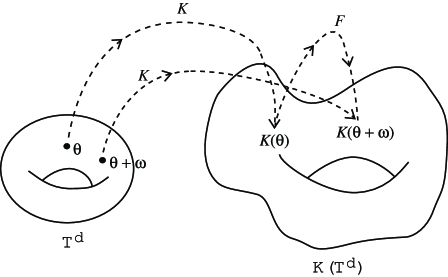
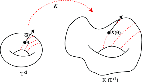
Figure 1. Illustration of the invariance equations (1), (2).

We go through a Newton scheme to prove the existence of such a pair $(\lambda,K)$. To this end, we introduce the operator $\mathcal{F}_{\omega}$

$$\mathcal{F}_{\omega}(\lambda,K)=F_{\lambda}\circ K-K\circ T_{\omega}.$$

In the paper [FdlLS09a], the authors constructed invariant tori using a posteriori KAM theorems in finite dimensional systems. The general principles of this method remain valid in some infinite dimensional systems such as lattices. We first introduce some notations and several non-degeneracy conditions.

Definition 3.1.

Consider $\rho>0,\ \omega\in{\mathbb{R}}^{l},\ \underline{c}=(c_{1},\dots,c_{R})\in({\mathbb{Z}}^{N})^{R},\ R\geq 1,$ a decay function $\Gamma,\ \lambda\in{\mathbb{R}}^{l}$ and $F_{\lambda}:{\mathcal{M}}\to{\mathcal{M}}$ be a $C^{2}_{\Gamma}$ map.

We say that $K:D_{\rho}\to{\mathcal{M}}\in\mathcal{A}_{\rho,\underline{c},\Gamma}$ is a whiskered embedding for $F_{\lambda}$ when we have:

The tangent space $T_{K(\theta)}{\mathcal{M}}$ has an invariant analytic splitting for all $\theta\in D_{\rho}$

(12) $$T_{K(\theta)}{\mathcal{M}}=\mathcal{E}^{s}_{{K(\theta)}}\oplus\mathcal{E}^{c}_{{K(\theta)}}\oplus\mathcal{E}^{u}_{{K(\theta)}}\,,$$

where $\mathcal{E}^{s}_{{K(\theta)}}$, $\mathcal{E}^{c}_{{K(\theta)}}$ and $\mathcal{E}^{u}_{{K(\theta)}}$ are the stable, center and unstable invariant spaces respectively, which satisfy:

• The projections $\Pi^{s}_{K(\theta)}$, $\Pi^{c}_{K(\theta)}$ and $\Pi^{u}_{K(\theta)}$ associated to this splitting are analytic with respect to $\theta$ considered as operators in ${\mathcal{L}}_{\Gamma}(\ell^{\infty}({\mathbb{Z}}^{N}))$.

• The splitting (12) is characterized by asymptotic growth conditions (co-cycles over $T_{\omega}$): there exist $0<\mu_{1},\mu_{2}<1$, $\mu_{3}>1$ such that $\mu_{1}\mu_{3}<1$, $\mu_{2}\mu_{3}<1$ and $C_{h}>0$ such that for all $n\geq 1$, $\theta\in D_{\rho}$ and $\lambda\in\mathbb{R}^{l}$

  (13) $$\begin{split}\|DF_{\lambda}&\circ K\circ T^{n-1}_{\omega}\times\dots\times DF_{\lambda}\circ Kv\|_{\rho,\underline{c},\Gamma}\leq C_{h}\mu_{1}^{n}\|v\|_{\rho,\underline{c},\Gamma}\\ &\iff v\in\mathcal{E}^{s}_{{K(\theta)}}\end{split}$$

  and

  (14) $$\begin{split}\|DF_{\lambda}^{-1}&\circ K\circ T^{-(n-1)}_{\omega}\times\dots\times DF_{\lambda}^{-1}\circ Kv\|_{\rho,\underline{c},\Gamma}\leq C_{h}\mu_{2}^{n}\|v\|_{\rho,\underline{c},\Gamma}\\ &\iff v\in\mathcal{E}^{u}_{{K(\theta)}}.\end{split}$$

• The center subspace $\mathcal{E}_{K(\theta)}^{c}$ is finite dimensional, has dimension $2l$ and it is characterized by:

  (15) $$\begin{split}\|DF_{\lambda}&\circ K\circ T^{n-1}_{\omega}(\theta)\times\dots\times DF_{\lambda}\circ K(\theta)v\|_{\rho,\underline{c},\Gamma}\leq C_{h}\mu_{3}^{n}\|v\|_{\rho,\underline{c},\Gamma}\\ \|DF_{\lambda}^{-1}&\circ K\circ T^{-(n-1)}_{\omega}(\theta)\times\dots\times DF_{\lambda}^{-1}\circ K(\theta)v\|_{\rho,\underline{c},\Gamma}\leq C_{h}\mu_{3}^{n}\|v\|_{\rho,\underline{c},\Gamma}\\ &\iff v\in\mathcal{E}^{c}_{{K(\theta)}}.\end{split}$$

It is important for applications that the spectral condition in Definition 3.1 is implied by a condition that can be verified by a finite calculation (see Definition 3.2 below). Approximate invariance of the splitting is sufficient (see Proposition 4.2 below) to ensure there is a truly invariant splitting. So, the final version of our results will have as a hypothesis the existence of approximately invariant tori with approximately invariant splitting (Definition 3.2). The final version of the results will have as a conclusion the existence of exactly invariant tori with exactly invariant splittings (Definition 3.1).

Definition 3.2.

Consider $\rho>0,\ \omega\in{\mathbb{R}}^{l},\ \underline{c}=(c_{1},\dots,c_{R})\in({\mathbb{Z}}^{N})^{R},\ R\geq 1,$ a decay function $\Gamma,\ \lambda\in{\mathbb{R}}^{l}$ and $F_{\lambda}:{\mathcal{M}}\to{\mathcal{M}}$ be a $C^{2}_{\Gamma}$ map.

We say that $\tilde{K}:D_{\rho}\to{\mathcal{M}}\in\mathcal{A}_{\rho,\underline{c},\Gamma}$ satisfies the $\eta$-hyperbolic condition (or has an $\eta-$invariant splitting), if there exists an analytic splitting of $T_{\tilde{K}({\mathbb{T}}^{l})}\mathcal{M}$,

(16) $$T_{\tilde{K}(\theta)}\mathcal{M}=\mathcal{E}^{s}_{{\tilde{K}(\theta)}}\oplus\mathcal{E}^{c}_{{\tilde{K}(\theta)}}\oplus\mathcal{E}^{u}_{{\tilde{K}(\theta)}}$$

such that, denoting $\Pi^{s,c,u}_{\tilde{K}(\theta)}$ be the corresponding projections, we have

1. The splitting is approximately invariant under the co-cycle $DF\circ{\tilde{K}}$ over $T_{\omega}$ in the sense that

   $${\rm dist}\Big{(}DF_{\lambda}(\tilde{K}(\theta))\mathcal{E}^{s,c,u}_{\tilde{K}(\theta)},\mathcal{E}^{s,c,u}_{\tilde{K}(\theta+\omega)}\Big{)}<\eta.$$

2. There exists $N\in{\mathbb{N}},0<\tilde{\mu}_{1},\tilde{\mu}_{2}<1$ and $\tilde{\mu}_{3}>1$ such that $\tilde{\mu}_{1},\tilde{\mu}_{3}<1,\ \tilde{\mu}_{2}\tilde{\mu}_{3}<1$ and

   (17) $$\begin{split}\|DF_{\lambda}&\circ\tilde{K}\circ T^{N-1}_{\omega}(\theta)\times\dots\times DF_{\lambda}\circ\tilde{K}(\theta)v\|_{\rho,\underline{c},\Gamma}\leq\tilde{\mu}_{1}^{N}\|v\|_{\rho,\underline{c},\Gamma},\\ &\forall v\in\mathcal{E}^{s}_{{\tilde{K}(\theta)}},\end{split}$$

   (18) $$\begin{split}\|DF_{\lambda}^{-1}&\circ\tilde{K}\circ T^{-(N-1)}_{\omega}(\theta)\times\dots\times DF_{\lambda}^{-1}\circ\tilde{K}(\theta)v\|_{\rho,\underline{c},\Gamma}\leq\tilde{\mu}_{2}^{N}\|v\|_{\rho,\underline{c},\Gamma},\\ &\forall v\in\mathcal{E}^{u}_{{\tilde{K}(\theta)}}\end{split}$$

   and

   (19) $$\begin{split}\|DF_{\lambda}&\circ\tilde{K}\circ T^{N-1}_{\omega}(\theta)\times\dots\times DF_{\lambda}\circ\tilde{K}(\theta)v\|_{\rho,\underline{c},\Gamma}\leq\tilde{\mu}_{3}^{N}\|v\|_{\rho,\underline{c},\Gamma}\\ \|DF_{\lambda}^{-1}&\circ\tilde{K}\circ T^{-(N-1)}_{\omega}(\theta)\times\dots\times DF_{\lambda}^{-1}\circ\tilde{K}(\theta)v\|_{\rho,\underline{c},\Gamma}\leq\tilde{\mu}_{3}^{N}\|v\|_{\rho,\underline{c},\Gamma}\\ &\forall v\in\mathcal{E}^{c}_{{\tilde{K}(\theta)}}.\end{split}$$

Remark 3.3.

Note that in Definition 3.2 we are using that the phase space is Euclidean. On a general manifold, the products used in (17), (18), (19) cannot be defined because, in general, $DF(x):T_{x}{\mathcal{M}}\rightarrow T_{F(x)}{\mathcal{M}}$. Hence, in a general manifold, if $F\circ K(\theta)\neq K(\theta+\omega)$, we cannot define $DF\circ K(\theta+\omega)DF\circ K(\theta)$. In [FdlLS09a] one can find a definition of approximately invariant cocycles for general manifolds. In this paper, we will not consider such generality.

We will define

$$\Omega^{c}_{K(\theta)}=\Omega|_{{\mathcal{E}}^{c}_{K(\theta)}}\quad\forall\theta\in{\mathbb{T}}^{\ell}$$

and we introduce the symplectic linear map $J^{c}(K(\theta)):{\mathcal{E}}^{c}_{K(\theta)}\rightarrow{\mathcal{E}}^{c}_{K(\theta)}$ by

$$\Omega^{c}_{K(\theta)}(u,v)=\langle u,J^{c}_{K(\theta)}v\rangle\quad\forall u,v\in{\mathcal{E}}^{c}_{K(\theta)}.$$

Obviously, we have $J^{c}(K(\theta))^{\top}=-J^{c}(K(\theta))$. We also have (See Lemma 4.8) that $\Omega^{c}$ is non-degenerate, hence $J^{c}$ is invertible.

Definition 3.4.

Given $\rho>0,\ \omega\in{\mathbb{R}}^{l},\ \underline{c}=(c_{1},\dots,c_{R})\in({\mathbb{Z}}^{N})^{R},\ R\geq 1,$ a decay function $\Gamma,\ \lambda\in{\mathbb{R}}^{l}$ and an embedding $K:D_{\rho}\rightarrow{\mathcal{M}}\in\mathcal{A}_{\rho,\underline{c},\Gamma}$, a pair $(\lambda,K)$ is said to be non-degenerate (and we denote $(\lambda,K)\in ND_{loc}(\rho,\Gamma)$) if it satisfies the following conditions

• Non degeneracy of the embedding: We have that the $l\times l$ matrix $DK^{\top}(\theta)DK(\theta)$ is invertible for all $\theta$ in $D_{\rho}$. We denote $N(\theta)=\big{(}DK^{\top}(\theta)DK(\theta)\big{)}^{-1}$ and we assume that

  $$\|N\|_{\rho,\Gamma}<\infty$$

• Twist condition: let $P(\theta)=DK(\theta)N(\theta)$.

  The average on ${\mathbb{T}}^{l}$ of the $l\times l-$matrix

  (20) $$A_{\lambda}(\theta)=P(\theta+\omega)^{\top}\Big{(}[DF_{\lambda}(K)(J^{c}\circ K)^{-1}P](\theta)-[(J^{c}\circ K)^{-1}P](\theta+\omega)\Big{)}$$

  is non-singular.

• Parameter cohomological non-degeneracy: The average on ${\mathbb{T}}^{l}$ of the $l\times l-$matrix

  (21) $$Q_{\lambda}(\theta)=\Big{(}(DK^{\top}(\omega+\theta)J^{c}(K(\omega+\theta))\frac{\partial F_{\lambda}(K(\theta))}{\partial\lambda}\Big{)}$$

  is non-singular.

It is clear that the meaning of $\|N\|_{\rho,\Gamma}$ is a measure of the quality of the embedding. It grows if the embedding comes close to having a singularity. During the proof it will become clear that the meaning of $A_{\lambda}$ is the change of the rotation when we move in the direction transversal to the torus. As we will see in calculations, the meaning of the invertibility of the average of $Q_{\lambda}$ is that, by changing $\lambda$, we can adjust the obstructions to the cohomology equations.

For applications, it is important to note that the non-degeneracy hypothesis only depend on the approximate solution considered and that they are readily computable algebraic expressions. They are quite analogous to the condition numbers in numerical analysis.

First we state our main theorem, which provides the existence of a solution $(\lambda,K)$ to the functional equation (11). This is the translated tori KAM theorem.

Theorem 3.5.

Let $F_{\lambda}:{\mathcal{M}}\rightarrow{\mathcal{M}}$ be a family of symplectic maps parameterized by $\lambda\in\mathbb{R}^{l}$, $\omega\in D(\kappa,\nu)$ for some $\kappa>0,\nu\geq l$, $\rho_{0}>0,\ \Gamma$ a decay function and $\underline{c}=(c_{1},\dots,c_{R})\in({\mathbb{Z}}^{N})^{R}$. Assume we have $\lambda_{0}\in{\mathbb{R}}^{l}$ and $K_{0}:D_{\rho}\supset{\mathbb{T}}^{l}\rightarrow{\mathcal{M}}$ satisfying the following hypotheses

• For all $\lambda\in{\mathbb{R}}^{l}$, the maps $F_{\lambda}$ belong to $C^{2}_{\Gamma}$ and satisfy $\sup_{i\in{\mathbb{Z}}^{N}}\Gamma^{-1}(i)(F_{\lambda}(0))_{i}<\infty$.

• The map $F_{\lambda}$ is real analytic and it can be extended holomorphically to some complex neighborhood of the image under $K_{0}$ of $D_{\rho_{0}}$:

  $$B_{r}=\left\{z\in{\mathcal{M}}|\;\exists\theta\quad s.t.\quad|\rm{Im}\,\,\theta|<\rho_{0}\ ,\ |z-K_{0}(\theta)|<r\right\},$$

  for some $r>0$ and such that $\|DF_{\lambda}\|_{C^{2}_{\Gamma}(B_{r})}$ is finite.

• $(\lambda_{0},K_{0})\in ND_{loc}(\rho_{0},\Gamma)$ i.e , the embedding $K_{0}$ is non-degenerate in the sense of Definition 3.4.

• The embedding $K_{0}$ is $\eta_{0}$-hyperbolic in the sense of Definition 3.2 with $\eta_{0}$ sufficiently small (depending on $\|\Pi^{s,c,u}\|_{\rho_{0},\underline{c},\Gamma}$, $\mu_{1,2,3}$, $N$, $\|F\|_{C^{2}_{\Gamma}(B_{r})}$).

Define the error $E_{0}$ by

$$E_{0}=F_{\lambda_{0}}\circ K_{0}-K_{0}\circ T_{\omega}.$$

Denote also

$${\tilde{\varepsilon}}=\max(\|E_{0}\|_{\rho_{0},\underline{c},\Gamma},\eta_{0}).$$

There exists a constant $C>0$ depending on $l$, $\kappa$, $\nu$, $\rho_{0}$, $\|DF_{\lambda}\|_{C_{\Gamma}^{2}(B_{r})}$, $\|DK_{0}\|_{\rho_{0},\underline{c},\Gamma}$, $\|N_{0}\|_{\rho_{0}}$, $\|\frac{\partial F_{\lambda}(K_{0})}{\partial\lambda}\|_{\rho_{0},\underline{c},\Gamma}$, $\|A_{\lambda_{0}}^{0}\|_{\rho_{0}}$, $|{\rm avg\,}(A_{\lambda_{0}}^{0})|^{-1}$, $|{\rm avg\,}(Q_{\lambda_{0}})|^{-1}$ (where $A_{\lambda_{0}}^{0}$, $Q_{\lambda_{0}}^{0}$ and $N_{0}$ are as in Definition 3.4, replacing $K$ with $K_{0}$) and on $\|\Pi^{c,s,u}_{K_{0}(\theta)}\|_{\rho_{0},\Gamma}$ such that, if for some $\delta$, $0<\delta<\min(1,\rho_{0}/12)$, we have the following conditions satisfied

$$C\kappa^{4}\delta^{-4\nu}{\tilde{\varepsilon}}<1$$

and

$$C\kappa^{2}\delta^{-2\nu}{\tilde{\varepsilon}}<r$$

then, there exist an embedding $K_{\infty}\in ND_{loc}(\rho_{\infty}=\rho_{0}-6\delta,\Gamma)$ and a vector $\lambda_{\infty}\in\mathbb{R}^{l}$ such that

(22) $$F_{\lambda_{\infty}}\circ K_{\infty}=K_{\infty}\circ T_{\omega}.$$

Furthermore, we have the following estimates

(23) $$\begin{split}&\|K_{\infty}-K_{0}\|_{\rho_{\infty},\underline{c},\Gamma}\leq C\kappa^{2}\delta^{-2\nu}{\tilde{\varepsilon}},\\ &|\lambda_{0}-\lambda_{\infty}|<C\kappa^{2}\delta^{-2\nu}{\tilde{\varepsilon}}.\end{split}$$

Additionnally, we have that the invariant embedding $K_{\infty}$ admits invariant splittings, satisfying Definition (3.4).

Denoting the non-degeneracy constants corresponding to $K_{\infty}$ by index $\infty$, we have:

(24) $$\begin{split}&\|\Pi^{s,c,u}_{\infty}\circ K_{\infty}-\Pi^{s,c,u}\circ K_{0}\|_{\rho_{\infty},\Gamma}\leq C\kappa^{2}\delta^{-2\nu}{\tilde{\varepsilon}},\\ &|\mu_{1,2,3}^{\infty}-\mu_{s,c,u}|\leq C\kappa^{2}\delta^{-2\nu}{\tilde{\varepsilon}}\end{split}$$

and

(25) $$\begin{split}&|\|N_{0}\|_{\rho_{0}}-\|N_{\infty}\|_{\rho_{\infty}}|\leq C\kappa^{2}\delta^{-2\nu}{\tilde{\varepsilon}},\\ &|\|A_{\lambda_{0}}^{0}\|_{\rho_{0}}-\|A_{\lambda_{\infty}}^{\infty}\|_{\rho_{\infty}}|\leq C\kappa^{2}\delta^{-2\nu}{\tilde{\varepsilon}},\\ &|\|Q_{\lambda}^{0}\|_{\rho_{0},\Gamma}-\|Q_{\lambda_{\infty}}^{\infty}\|_{\rho_{\infty},\Gamma}|\leq C\kappa^{2}\delta^{-2\nu}{\tilde{\varepsilon}}.\\ \end{split}$$

The previous theorem will allow us to construct increasingly complicated solutions, the solutions of one stage being an approximate solution for the next stage. We will however be able to maintain enough control of the non-degeneracy conditions.

Of course, (25) is an easy consequence of (23) since the objects that enter in the degeneracy estimates are algebraic expressions of $K$.

We now come to the result on the existence of invariant tori. They correspond to localized quasi-periodic orbits on the manifold ${\mathcal{M}}$. These orbits are known as “breathers”.

Theorem 3.6.

Let $F_{\lambda}:{\mathcal{M}}\rightarrow{\mathcal{M}}$ be a family of symplectic maps parameterized by $\lambda\in\mathbb{R}^{l}$, $\omega\in D(\kappa,\nu)$ for some $\kappa>0,\nu\geq l$, $\rho_{0}>0,\ \Gamma$ a decay function and $\underline{c}=(c_{1},\dots,c_{R})\in({\mathbb{Z}}^{N})^{R}$. Assume we have $\lambda_{0}\in{\mathbb{R}}^{l}$ and $K_{0}:D_{\rho}\supset{\mathbb{T}}^{l}\rightarrow{\mathcal{M}}$ satisfying the following hypotheses

• The map $F_{\lambda_{0}}$ is exact symplectic and $F_{\lambda_{0}}(0)=0$.

• For all $\lambda\in{\mathbb{R}}^{l}$, the maps $F_{\lambda}$ belong to $C^{2}_{\Gamma}$ and satisfy $\sup_{i\in{\mathbb{Z}}^{N}}\Gamma^{-1}(i)(F_{\lambda}(0))_{i}<\infty$.

• The map $F_{\lambda}$ is real analytic and it can be extended holomorphically to some complex neighborhood of the image under $K_{0}$ of $D_{\rho_{0}}$:

  $$B_{r}=\left\{z\in{\mathcal{M}}|\;\exists\theta\quad s.t.\quad|\rm{Im}\,\,\theta|<\rho_{0}\ ,\ |z-K_{0}(\theta)|<r\right\},$$

  for some $r>0$ and such that $\|DF_{\lambda}\|_{C^{2}_{\Gamma}(B_{r})}$ is finite.

• $(0,K_{0})\in ND_{loc}(\rho_{0},\Gamma)$ i.e , the embedding $K_{0}$ is non-degenerate in the sense of Definition3.4.

• The embedding $K_{0}$ is $\eta_{0}$-hyperbolic in the sense of Definition 3.2 with $\eta_{0}$ sufficiently small (depending on $\|\Pi^{s,c,u}\|_{\rho_{0},\Gamma}$, $\mu_{1,2,3}$, $N$, $\|F\|_{C^{2}_{\Gamma}(B_{r})}$).

Define the error $E_{0}$ by

$$E_{0}=F_{\lambda_{0}}\circ K_{0}-K_{0}\circ T_{\omega}.$$

Denote also

$${\tilde{\varepsilon}}=\max(\|E_{0}\|_{\rho_{0},\underline{c},\Gamma},\eta_{0}).$$

There exists a constant $C>0$ depending on $l$, $\kappa$, $\nu$, $\rho_{0}$, $\|DF_{\lambda}\|_{C_{\Gamma}^{2}(B_{r})}$, $\|DK_{0}\|_{\rho_{0},\underline{c},\Gamma}$, $\|N_{0}\|_{\rho_{0}}$, $\|\frac{\partial F_{\lambda}(K_{0})}{\partial\lambda}\|_{\rho_{0},\underline{c},\Gamma}$, $\|A_{0}^{0}\|_{\rho_{0}}$, $|{\rm avg\,}(A_{0}^{0})|^{-1}$, $|{\rm avg\,}(Q_{0})|^{-1}$ (where $A_{0}^{0}$, $Q_{0}^{0}$ and $N_{0}$ are as in Definition 3.4, replacing $K$ with $K_{0}$) and on $\|\Pi^{c,s,u}_{K_{0}(\theta)}\|_{\rho_{0},\underline{c},\Gamma}$ such that, if for some $\delta$, $0<\delta<\min(1,\rho_{0}/12)$, we have the following conditions satisfied

$$C\kappa^{4}\delta^{-4\nu}{\tilde{\varepsilon}}<1$$

and

$$C\kappa^{2}\delta^{-2\nu}{\tilde{\varepsilon}}<r$$

Then, we have in (22)

$$\lambda_{\infty}=0,$$

i.e. the torus $K_{\infty}$ is actually an invariant torus for $F_{\lambda_{0}}$ and we have

$$F_{\lambda_{0}}\circ K_{\infty}=K_{\infty}\circ T_{\omega}.$$

Remark 3.7.

It is important to mention that we do not assume that the symplectic forms are the standard ones. This allows to consider the existence of external magnetic fields and magnetic interactions among the sites since the effect of a magnetic field is just a change of the symplectic form [Thi97]. Alternatively, if $(p,q)$ are the conjugated coordinates, one can change $p\to p-A$ where $A$ is the vector potential. Note that the introduction of a magnetic field destroys the reversibility under the usual involution $S(p,q)=(-p,q)$.

Remark 3.8.

The whiskered tori that satisfy the spectral hypothesis have invariant manifolds that make them important in problems of stability. However, the proof of the stable manifold is not completely straightforward since the space $\ell^{\infty}$ does not have smooth cut-off functions. It is possible to show that these invariant manifolds have also some decay properties. This has been established in [FdlLM11b].

We have also the following result which provides local uniqueness.

Theorem 3.9.

Let $\omega\in D(\kappa,\nu)$ for some $\kappa>0,\nu>l$ and $K_{1}\in ND(\rho)$ and $K_{2}\in ND(\rho)$ be two solutions of equation (1) such that $K_{1}(D_{\rho})\subset B_{r},\,K_{2}(D_{\rho})\subset B_{r}$. There exists a constant $C>0$ depending on $l$, $\kappa$, $\nu$, $\rho$, $\rho^{-1}$, $\|F\|_{C^{2}_{\Gamma}}$, $\|K_{1}\|_{\rho,\underline{c},\Gamma}$, $\|N_{1}\|_{\rho,\Gamma}$, $\|A_{1}\|_{\rho,\Gamma}$, $|{\rm avg\,}(A_{1})|^{-1}$ such that if $\|K_{1}\circ T_{\tau}-K_{2}\|_{\rho,\underline{c},\Gamma}$ satisfies for some $\tau\in\mathbb{R}^{l}$

$$C\kappa^{2}\delta^{-2\nu}\|K_{1}\circ T_{\tau}-K_{2}\|_{\rho_{0},\underline{c},\Gamma}\leq 1,$$

where $\delta=\rho/4$, then there exists a phase $\tilde{\tau}\in\mathbb{R}^{l}$ such that $K_{1}\circ T_{\tilde{\tau}}=K_{2}$ in $D_{\rho}$. Moreover,

$$|\tau-\tilde{\tau}|\leq C\kappa^{2}\rho^{-2\nu}\|K_{1}\circ T_{\tau}-K_{2}\|_{\rho_{0},{\underline{c}}\Gamma}.$$

Remark 3.10.

It is important to remark that ALL constants in the previous theorems are independent of $\underline{c}$. This fact is crucial for the next result, which provides an existence theorem for almost-periodic functions.

The idea of the construction follows the one in the finite dimensional case (see [FdlLS09a]). Notice here that the decay properties are on the hyperbolic subspace, the center one being finite dimensional. Some small differences between the scheme of the present paper and [FdlLS09a] are detailed in Remark 4.20.

We also have the analogous result to Theorem 3.6 for vector-fields, Theorem 8.4. We will postpone the statement of Theorem 8.4 till Section 8 where we also present a proof.

As an application of Theorem 8.4, we will present a result on existence of solutions with infinitely many frequencies (also called almost periodic solutions). We note that, as indicated before, we will establish the theorem in two stages. In a first stage, we will continue the breathers from the uncoupled system to the whole system. In the second stage, we will couple infinitely many of these breathers so that we obtain solutions with infinitely many frequencies. We note that the smallness conditions and the elimination of a positive measure set of frequencies only occurs in the first stage. In the second stage, we only need to eliminate a zero measure set of frequencies (in many different measures) and we do not need any smallness condition. The reason is that in the second stage, we adjust all the smallness conditions by placing the individual breathers far enough. Of course, if we wanted to let the breathers not to be so far appart, it could be done with other assumptions.

The models we consider (26) have been considered in the Physics and Mathematics literature. They are models of many microscopic processes. See [BK04, BK98, DRAW02, FBGGn05, CF05, Gal08, BEMW07] and references there among many others.

A large variety of solutions for equations of this type have been constructed: space-localized periodic in time solutions, known as breathers (see [MA94, Jam01]), solitary waves ([Ioo00, IK00, FW94], [FP99, FP02, FP04a, FP04b]), pulsating traveling waves (see [JS05, Sir05]). The relevance of these solutions in biological phenomena has also been discussed (see [DPW92, PS04, Pey04]).

There are already several other papers that have produced solutions with infinitely many frequencies. The paper [FSW86] produced such solutions by introducing some random terms and making the excitation of each oscillator goes to zero, so that its effect on the others was small. Frölich, Spencer and Wayne also assume that the coupling is high order in terms of the amplitude. The paper [CP95, Per03] considered oscillators but made the natural frequencies increase very fast so that there were no resonances in each of them. The paper [Pös90] proved a very abstract theorem that applies to perturbations of integrable systems and managed to recover several results as applications of this theorem. The paper [GY07] also considers coupled systems in one dimension, but produces tori with finitely many frequencies.

The solutions we construct are based on a different principle. We use that the solutions which are far apart interact very weakly even if they are large. Therefore, by placing solutions far apart, we will be able to make them interact weakly and we can satisfy the smallness conditions assumed by the general theorem. Notice that we are assuming that most of the sites are close to a hyperbolic orbit. Hence, the system will be very hyperbolic. This will allow us to deal with most of the normal directions using the methods of hyperbolic splittings and we will not need to consider the resonances that appear in the normally elliptic modes, which require more delicate estimates. We emphasize that we do not assume that the system is close to integrable.

Theorem 3.11.

Consider a lattice ${\mathcal{M}}=M^{{\mathbb{Z}}^{N}}$ with the symplectic form given by $\Omega_{\infty}=\sum_{n\in{\mathbb{Z}}^{N}}dq_{n}\wedge dp_{n}$. Consider the following Hamiltonian with respect to $\Omega_{\infty}$ given by

(26) $$H(q,p)=\sum_{n\in{\mathbb{Z}}^{N}}\Big{(}\frac{1}{2}\,|p_{n}|^{2}+W(q_{n})\Big{)}+\varepsilon\sum_{j\in{\mathbb{Z}}^{N}}\ \sum_{n\in{\mathbb{Z}}^{N}}V_{j}(q_{n}-q_{n+j}).$$

Let $\Gamma,\Gamma^{\prime}$ be decay functions as in Proposition 2.3.

Denote by $X$ the vector field associated to the Hamiltonian (26).

Assume:

1. The system $\ddot{q}+W^{\prime}(q)=0$ admits a hyperbolic fixed point, which we will set without loss of generality at $q=0$.

2. There exists a set $\Xi_{0}\subset{\mathbb{R}}^{l}$ of positive Lebesgue measure such that for all $\omega\in\Xi_{0}$, there exists a KAM torus invariant under the flow of $\ddot{q}+W^{\prime}(q)=0$ and non-degenerate in the sense of the standard KAM theory (twist condition).

3. The potentials $V_{j}$ and $W$ are real analytic. Moreover, we assume that there exists a constant $C_{V}$ such that

   $$\|V_{k}\|_{C^{2},\rho}\leq C_{V}\Gamma(k).$$

   and also that $\nabla V_{k}(0)=0$ for every $k$.

Fix $\rho^{\prime}<\rho$. Then,

1. A)For all $\varepsilon^{*}$ sufficiently small, we can find a set $\Xi_{1}(\varepsilon^{*})\subset\Xi_{0}$, such that if $\omega\in\Xi_{1}(\varepsilon^{*})$ and $|\varepsilon|<\varepsilon^{*}$, then the system (26) has a localized breather of frequency $\omega$. There exists $K:{\mathbb{T}}^{l}\rightarrow{\mathcal{M}}$, $K\in A_{\rho^{\prime},\underline{c},\Gamma}$ such that

   $$X\circ K=\partial_{\omega}K$$

   The embedding satisfies Definition 3.1 and we can choose the hyperbolicity and non-degeneracy constants uniformly.

   Furthermore we have

   $${\rm meas}({\Xi_{0}\setminus\Xi_{1}(\varepsilon^{*})})\to 0$$

   as $\varepsilon^{*}\to 0$.

2. B) Consider now $\Xi_{\infty}=\Xi_{1}(\varepsilon^{*})^{\mathbb{N}}$ endowed with the probability measure $\Big{(}\frac{{\rm meas}(\cdot)}{{\rm meas}({\Xi_{1}(\varepsilon^{*})}}\Big{)}^{\mathbb{N}}$. Then, there exists a set $\Xi_{\infty}^{*}\subset\Xi_{\infty}$, ${\rm meas}(\Xi_{\infty}^{*})=1$, such that if $\underline{\omega}\in\Xi^{*}_{\infty}$, there exist a sequence of centers $\underline{c}$ and a $K$ analytic in some strip of $({\mathbb{T}}^{l})^{\mathbb{N}}$ so that

   $$J_{\infty}\nabla H\circ K=\partial_{\underline{\omega}}K.$$

Note that we have stated Theorem 3.11 only for decay functions of the form given in Proposition 2.3. It is clear that the proof only uses a few properties of the function (e.g. monotonicity in the modulus of the argument). We have refrained from reformulating the theorem in more abstract terms.

We note that the only smallness conditions in $\varepsilon$ enter just in the first stage of creating individual breathers around each site and in the preservation of the hyperbolic structure and other non-degeneracy conditions. The second stage, on the other hand does not require any other smallness conditions.

In the construction of infinite dimensional breathers out of single breathers we just need to exclude a few sequences of frequencies which are very resonant (they have measure zero in the probability measure indicated above). See Section 9.3. The smallness assumptions that we need to couple the sequences can be adjusted just by placing the different breathers far apart and we do not need any further smallness conditions in $\varepsilon$.

Note also that the only hypothesis on the one site system is the existence of positive measure of KAM tori (and the existence of a hyperbolic fixed point). This is implied if the system is close to a non-degenerate integrable system. Nevertheless, there are other arguments to show existence of KAM tori in systems very far from integrable [Dua94, Dua08]. Any of these systems could be taken as the basis for Theorem 3.11.

4. The Newton step

The sketch of the proof of Theorem 3.5 is roughly the same as for finite dimensional systems, with some minor changes detailed in Remark 4.20. Of course, even if the strategy is similar to that in finite dimensions, all the details need to be different since the situation is very different and we need to pay attention to the decay properties. With a view to applications to almost periodic solutions of Theorem 3.11, we also need to pay attention to the change in the non-degeneracy conditions and in the hyperbolicity properties and establish that many of the smallness assumptions are independent of the number and the geometry of the centers of oscillation.

The proof of Theorem 3.5 is based on a Newton iteration of Nash-Moser type. The estimates of the Newton step – including uniqueness – are summarized in Section 4.1 (See, Lemma 4.1). The fact that the inductive step can be iterated is more or less standard in KAM theory and it is done in Section 5.

The proof of the estimates of the Newton step are obtained in different stages

1. We show that the approximate invariant hyperbolic splitting can be transformed in an invariant splitting. See Section 4.2.

2. The equations for the Newton step can be divided into equations along the hyperbolic spaces (studied in Section 4.4) and the center space (studied in Section 4.3).

   As usual in the study of cohomology equations, the equations in the center direction are much more subtle. In particular, the Diophantine properties and the geometric properties are only used in the equations in the center space.

3. Once we have the estimates for the approximate solutions of the linearized equation, we show that, using the linearized equation, they improve the solutions of the translated equation. Furthermore, we estimate the changes in the hyperbolicity constants and the non-degeneracy estimates.

4. The passage from Theorem 3.5 to Theorem 3.6 is a geometric argument (a vanishing lemma) undertaken in Section 6.

4.1. Estimates for the inductive step

In this section we describe the inductive step of the proof of Theorem 3.5.

By Taylor’s theorem we can write

$$\mathcal{F}_{\omega}(\lambda+\Lambda,K+\Delta)=\mathcal{F}_{\omega}(\lambda,K)+D_{\lambda,K}\mathcal{F}_{\omega}(\lambda,K)(\Lambda,\Delta)+O(|(\Lambda,\Delta)|^{2}).$$

Assuming that $(\lambda,K)$ is a pair that satisfies ${\mathcal{F}}_{\omega}(\lambda,K)=0$ approximately with an error $E(\theta)={\mathcal{F}}_{\omega}(\lambda,K)(\theta)$ we look for $(\Lambda,\Delta)$ such that ${\mathcal{F}}_{\omega}(\lambda+\Lambda,\,K+\Delta)$ is as small as possible. Then we are lead to consider the following Newton equation

(27) $$D_{\lambda,K}\mathcal{F}_{\omega}(\lambda,K)(\Lambda,\Delta)=-E,$$

where

$$\begin{split}D_{\lambda,K}&\mathcal{F}_{\omega}(\lambda,K)(\Lambda,\Delta)(\theta)=\frac{\partial F_{\lambda}(K(\theta))}{\partial\lambda}\Lambda+DF_{\lambda}(K(\theta))\Delta(\theta)-\Delta(\theta+\omega).\end{split}$$

To solve (27) we project the equation on both the center and the hyperbolic subspaces, taking advantage of the invariant splitting. Then we try to solve the projected equations. The one on the center subspace is reduced to two small divisors equations, essentially one on the tangent of the torus and the other on its conjugated directions. Taking advantage of the extra variable $\lambda$, we can solve these equations up to a quadratic error. Using the conditions on the co-cycles over $T_{\omega}$, we solve the projection on the stable and unstable subspaces.

The next result gives an approximate solution of (27) with precise estimates.

Lemma 4.1.

Under the hypotheses of Theorem 3.5 the equation

$$D_{\lambda,K}\mathcal{F}_{\omega}(\lambda,K)(\Lambda,\Delta)=-E$$

has an approximate solution $(\Lambda,\Delta)$ in the following sense: let

$$\tilde{E}=D_{\lambda,\kappa}\,{\mathcal{F}}_{\omega}(\lambda,K)\,(\Lambda,\Delta)+E\,.$$

For $0<\delta<\rho$ we have the following estimates

$$\|\Delta\|_{\rho-\delta,\underline{c},\Gamma}\leq C\kappa^{2}\delta^{-2\nu}\|E\|_{\rho,\underline{c},\Gamma},$$

$$|\Lambda|\leq C\|E\|_{\rho,\underline{c},\Gamma},$$

$$\|\tilde{E}\|_{\rho-\delta,\underline{c},\Gamma}\leq C\kappa^{2}\delta^{-(2\nu+1)}\|E\|_{\rho,\underline{c},\Gamma}\|\mathcal{F}_{\omega}(\lambda,K)\|_{\rho,\underline{c},\Gamma}.$$

Moreover, if $\Delta$ and $\tilde{\Delta}$ are solutions of (27) as above, i.e. solutions with quadratic error bounded by $C\kappa^{2}\delta^{-(2\nu+1)}\|E\|_{\rho,\underline{c},\Gamma}\ \|{\mathcal{F}}_{\omega}\|_{\rho,\underline{c},\Gamma}$,

$$\|\Delta-\tilde{\Delta}-DK(\theta)\alpha\|_{\rho-\delta,\underline{c},\Gamma}\leq C\kappa^{2}\delta^{-(2\nu+1)}\|E\|_{\rho,\underline{c},\Gamma}\|\mathcal{F}_{\omega}(\lambda,K)\|_{\rho,\underline{c},\Gamma}.$$

In the previous estimates, the constant $C$ depends on $\rho,l,\|DK\|_{\rho,\underline{c},\Gamma},$ $\|\Pi^{s,c,u}_{K(\theta)}\|_{\rho,\Gamma},$ $\|\frac{\partial F_{\lambda}}{\partial\lambda}\|_{\rho,\underline{c},\Gamma}$, the hyperbolicity constants and the decay function $\Gamma$ but it does not depend on $\underline{c}$.

4.2. Construction of invariant splittings out of approximately invariant ones

The main result of this section will be Proposition 4.2, which establishes that given an approximately invariant splitting satisfying Definition 3.1, there is a truly invariant splitting nearby. Furthermore, we can estimate the distance between the true invariant splitting and the approximately invariant one. This, of course, implies the usual formulation of persistence of splittings under small perturbations.

The way that this result fits into the Newton scheme is that this will allow us to split the equation into different components. Compared to other estimates in the Newton step, the construction of invariant splittings requires much less sophisticated analysis (it suffices to use contractions) and it does not require inductive assumptions nor making choices (e.g. the domain loss). The subtlety of the results comes because we have to choose appropriate spaces so that the estimates are uniform in the domains, the arrangement of the centers, etc. This uniformity of the results will be used when we consider the limit of infinitely many frequencies.

The method of proof we use is very similar to the standard proof using graph transforms [HP70, HPS77], which adapts very well to infinite dimensions [PS99]. Of course, there are several subtleties due to the infinite dimensional nature of the problem. In particular, we make essential use of the Banach algebra properties of the decay functions to make sure that we obtain estimates in the same spaces of functions (it is interesting to compare this with previous results in lattice dynamical systems). We emphasize that, in particular, the smallness conditions are independent of the centers of the embedding. This will be crucial when we consider the limit of a large number of centers.

Proposition 4.2.

Assume that the embedding $\tilde{K}$ has a $\delta$-invariant hyperbolic splitting $\tilde{\mathcal{E}}^{s},\tilde{\mathcal{E}}^{c},\tilde{\mathcal{E}}^{u}$ with respect to a map $F$ (See Definition 3.2). Denote by $\tilde{\Pi}^{\sigma}$, $\sigma=s,c,u$ the projections corresponding to this splitting.

There exists $\delta_{0}>0$ depending on $\|N\|_{\rho,\Gamma},\|DF\circ\tilde{K}\|_{\rho,\underline{c},\Gamma},\|DF^{-1}\circ\tilde{K}\|_{\rho,\underline{c},\Gamma}$ and $\|\Pi^{s,c,u}\|_{\rho,\underline{c},\Gamma}$, $\mu_{s,c,u}$ such that if $0<\delta<\delta_{0}$ there is an analytic splitting

(28) $$T_{\tilde{K}(\theta)}{\mathcal{M}}=\mathcal{E}^{s}_{\tilde{K}(\theta)}\oplus\mathcal{E}^{c}_{\tilde{K}(\theta)}\oplus\mathcal{E}^{u}_{\tilde{K}(\theta)}$$

which is invariant under the co-cycle $DF\circ\tilde{K}$ over $T_{\omega}$.

Let $\tilde{\Pi}^{s,c,u}_{\tilde{K}(\theta)}$ be the projections corresponding to the splitting (28). We furthermore have that there exist $C_{h},0<\mu_{1},\mu_{2}<1,\,\mu_{3}>1$ such that $\mu_{1}\mu_{3}<1,\,\mu_{2}\mu_{3}<1$ and the characterizations (13), (14), (15) of the splitting hold.

Moreover, there exists $C>0$, depending on the same quantities as $\delta_{0}$ does, such that for $0<\delta<\delta_{0}$

$$\|\Pi^{s,c,u}_{\tilde{K}(\theta)}-\tilde{\Pi}^{s,c,u}_{\tilde{K}(\theta)}\|_{\rho,\Gamma}\leq C\delta,$$

$$|\mu_{1,2,3}-\tilde{\mu}_{1,2,3}|<C\delta.$$

Proof.

The ideas in this proof follow the ones in [FdlLS09a]. They have been taken from [HPPS70]. We make sure that the estimates are uniform with respect to $\delta$ and $\underline{c}$. We divide the proof into several steps.

Step 1: Construction of the invariant spaces. The existence of the invariant splitting will be done through the Banach fixed point principle applied to a graph transform operator.

We begin with the case of the stable bundle ${\mathcal{E}}^{s}_{\tilde{K}(\theta)}$. We describe the stable space ${\mathcal{E}}^{s}_{\tilde{K}(\theta)}$ as the graph of a linear map, i.e. ${\mathcal{E}}^{s}_{\tilde{K}(\theta)}=\mbox{graph}\,(u\circ\tilde{K})$, where $u\circ\tilde{K}$ maps $\mathcal{\tilde{E}}^{s}_{{\tilde{K}}(\theta)}$ linearly into $\mathcal{\tilde{E}}^{c}_{{\tilde{K}}(\theta)}\oplus\mathcal{\tilde{E}}^{u}_{{\tilde{K}}(\theta)}$.

Since the splitting (16) is approximately invariant we can write the matrix $DF\big{(}\tilde{K}(\theta)\big{)}$ with respect to this decomposition as

$$DF\big{(}\tilde{K}(\theta)\big{)}=\begin{pmatrix}a_{11}(\theta)&a_{12}(\theta)\\ a_{21}(\theta)&a_{22}(\theta)\end{pmatrix}$$

with $\|a_{12}\|_{\rho,\underline{c},\Gamma}<C\delta,\ \|a_{21}\|_{\rho,\underline{c},\Gamma}<C\delta.$ We also write

$$DF\big{(}\tilde{K}(\theta+(N-1)\,\omega)\big{)}\times\dots\times DF\big{(}\tilde{K}(\theta)\big{)}=\begin{pmatrix}a_{11}^{N}(\theta)&a_{12}^{N}(\theta)\\ a_{21}^{N}(\theta)&a_{22}^{N}(\theta)\end{pmatrix}.$$

Note that by (17), (18) and (19) we have

(29) $$\|a_{11}^{N}\|_{\rho,\underline{c},\Gamma}\leq(1+C\delta)\mu^{N}_{1}\,,\qquad\|a_{22}^{-N}\|_{\rho,\underline{c},\Gamma}\leq(1+C\delta)\mu^{N}_{3}\,,$$

and

(30) $$\|a_{12}^{N}\|_{\rho,\underline{c},\Gamma}\leq C\delta\,,\qquad\|a_{21}^{N}\|_{\rho,\underline{c},\Gamma}\leq C\delta\,.$$

The graph condition over the co-cycle is

$$DF\circ\tilde{K}(\theta)\begin{pmatrix}{\rm Id}\\ u\circ\tilde{K}(\theta)\end{pmatrix}\in\mbox{graph}\Big{(}u\circ\tilde{K}\big{(}T_{\omega}(\theta)\big{)}\Big{)}.$$

This gives the functional equation for the map $u$

(31) $$u\circ\tilde{K}\big{(}T_{\omega}(\theta)\big{)}(a_{11}+a_{12}\ u\circ\tilde{K})(\theta)=(a_{21}+a_{22}\ u\circ\tilde{K})\,(\theta)\,.$$

Denoting $\tilde{u}=u\circ\tilde{K}\,$, (31) can be rewritten as

(32) $$\tilde{u}=a_{22}^{-1}\big{[}\tilde{u}\circ T_{\omega}(a_{11}+a_{12}\,\tilde{u})-a_{21}\big{]}.$$

Let ${\mathcal{L}}_{\eta}$ be the ball of radius $\eta$ in the space of linear operators from $\mathcal{\tilde{E}}^{s}_{\tilde{K}(\theta)}$ into $\mathcal{\tilde{E}}^{c}_{\tilde{K}(\theta)}\oplus\mathcal{\tilde{E}}^{u}_{\tilde{K}(\theta)}$ with the norm $\|\cdot\|_{\Gamma}$.

Let ${\mathcal{S}}_{\eta}$ be the space of analytic sections from $D_{\rho}$ to ${\mathcal{L}}_{\eta}$, i.e. the space of $u:D_{\rho}\to{\mathcal{L}}_{\eta}$ such that $u(\theta):\mathcal{\tilde{E}}^{s}_{\tilde{K}(\theta)}\to\mathcal{\tilde{E}}^{c}_{\tilde{K}(\theta)}\oplus\mathcal{\tilde{E}}^{u}_{\tilde{K}(\theta)}$ with the norm $\|.\|_{\rho,\Gamma}$.

We take the operator ${\mathcal{T}}:{\mathcal{S}}_{\eta}\to{\mathcal{S}}_{\eta}$ defined as the right-hand side of (32). ${\mathcal{T}}$ is approximated by ${\mathcal{T}}_{0}:{\mathcal{S}}_{\eta}\to{\mathcal{S}}_{\eta}$ defined by

$${\mathcal{T}}_{0}\,\tilde{u}=a^{-1}_{22}\ \tilde{u}\circ T_{\omega}\ a_{11}.$$

We now consider ${\mathcal{T}}^{N}$ and ${\mathcal{T}}_{0}^{N}$. An elementary computation gives

$${\mathcal{T}}^{N}_{0}\,\tilde{u}=a^{-1}_{22}\dots a^{-1}_{22}\circ T^{N-1}_{\omega}\,\tilde{u}\circ T^{N}_{\omega}\ a_{11}\circ T^{N-1}_{\omega}\dots\,a_{11\,.}$$

Moreover, taking into account that ${\mathcal{T}}$ is a degree two polynomial operator, we obtain by simple algebraic manipulations

(33) $$\|{\mathcal{T}}^{N}-{\mathcal{T}}^{N}_{0}\|<C\delta$$

and

(34) $$\mbox{Lip}({\mathcal{T}}^{N}-{\mathcal{T}}^{N}_{0})<C\delta\,.$$

Using the Banach algebra properties of the decay norms, we have that

(35) $$\|a^{N}_{11}(\theta)-a_{11}\big{(}T^{N-1}_{\omega}(\theta)\big{)}\dots a_{11}(\theta)\|_{\rho,\underline{c},\Gamma}<C\delta\,,$$

(36) $$\|a^{-N}_{22}(\theta)-a_{22}^{-1}(\theta)\dots a^{-1}_{22}\big{(}T^{N-1}_{\omega}(\theta)\big{)}\|_{\rho,\underline{c},\Gamma}<C\delta\,.$$

By (29), (35) and (36), if $\delta$ is small, ${\mathcal{T}}^{N}_{0}$ sends ${\mathcal{S}}_{\eta}$ into ${\mathcal{S}}_{\eta}$ for all $\eta\in(0,1]$ and is a contraction in this domain. By (33) and (34), if $\delta$ is small ${\mathcal{T}}^{N}$ sends ${\mathcal{S}}_{\eta}$ into ${\mathcal{S}}_{\eta}$ for $\eta\in(C\delta,1]$ and it is also a contraction.

Therefore ${\mathcal{T}}^{N}$ has a unique fixed point $u^{*}$ in ${\mathcal{S}}_{1}$ which belongs to ${\mathcal{S}}_{C\delta}$. It is clear that ${\mathcal{T}}u^{*}$ is also a fixed point of ${\mathcal{T}}^{N}$, which belongs to ${\mathcal{S}}_{C^{\prime}\delta}\ \subset{\mathcal{S}}_{1}$ for some $C^{\prime}\geq C$. By uniqueness ${\mathcal{T}}u^{*}=u^{*}$.

A similar method can be applied for the center-unstable subspace. In this case the graph condition reads

$$DF_{\lambda}\circ\tilde{K}(\theta)\begin{pmatrix}v\circ\tilde{K}(\theta)\\ {\rm Id}\end{pmatrix}\in\mbox{graph}\Big{(}v\circ\tilde{K}\big{(}T_{\omega}(\theta)\big{)}\Big{)},$$

and the resulting operator ${\mathcal{T}}:\mathcal{S}_{\eta}\rightarrow\mathcal{S}_{\eta}$ is

(37) $${\mathcal{T}}\tilde{v}=\big{[}(\tilde{a}_{11}\tilde{v}+\tilde{a}_{12})(\tilde{a}_{21}\tilde{v}+\tilde{a}_{22})^{-1}\big{]}\circ T^{-1}_{\omega},$$

where $\tilde{v}=v\circ\tilde{K}$. Repeating the same procedure as above, we construct the center-unstable space and obtain similar bounds.

Now let us consider $G=F^{-1}$. We observe that the stable space associated to the map $G$ is the unstable space associated to $F$. Hence, applying the above procedure to $G$, we construct the unstable space ${\mathcal{E}}^{u}_{\tilde{K}(\theta)}$ and center-stable space ${\mathcal{E}}^{c,s}_{\tilde{K}(\theta)}$ with similar bounds. Finally we note that ${\mathcal{E}}^{c}_{\tilde{K}(\theta)}={\mathcal{E}}^{c,s}_{\tilde{K}(\theta)}\bigcap{\mathcal{E}}^{c,u}_{\tilde{K}(\theta)}$.

Step 2: Estimates on the projections. We want to estimate the norm of the projection $\Pi^{s}_{\tilde{K}(\theta)}$ compared to the one of $\tilde{\Pi}^{s}_{\tilde{K}(\theta)}$.

Let $\xi\in T_{\tilde{K}(\theta)}{\mathcal{M}}$. Using the decomposition $\xi=(\xi^{s},\xi^{cu})\in\mathcal{E}^{s}_{\tilde{K}(\theta)}\oplus(\mathcal{E}^{c}_{\tilde{K}(\theta)}\oplus\mathcal{E}^{u}_{\tilde{K}(\theta)})$ we have the following representations

$${\tilde{\Pi}}^{s}_{\tilde{K}(\theta)}\xi=(\xi^{s},0), \qquad\Pi^{s}_{\tilde{K}(\theta)}\xi=(\tilde{\xi}^{s},\tilde{u}(\theta)\tilde{\xi}^{s}),$$

$$\tilde{\Pi}^{cu}_{\tilde{K}(\theta)}\xi=(0,\xi^{cu}), \qquad\Pi^{cu}_{\tilde{K}(\theta)}\xi=(\tilde{v}(\theta)\tilde{\xi}^{cu},\tilde{\xi}^{cu}).$$

Then

$$\xi^{s} =\tilde{\xi}^{s}+\tilde{v}(\theta)\tilde{\xi}^{cu},$$

$$\xi^{cu} =\tilde{u}(\theta)\tilde{\xi}^{s}+\tilde{\xi}^{cu}$$

or equivalently

$$\left(\begin{array}[]{c}\tilde{\xi}^{s}\\ \tilde{\xi}^{cu}\end{array}\right)=\left(\begin{array}[]{cc}{\rm Id}&\tilde{v}(\theta)\\ \tilde{u}(\theta)&{\rm Id}\end{array}\right)^{-1}\left(\begin{array}[]{c}\xi^{s}\\ \xi^{cu}\end{array}\right)$$

since the matrix $B=\left(\begin{array}[]{cc}{\rm Id}&\tilde{v}(\theta)\\ \tilde{u}(\theta)&{\rm Id}\end{array}\right)$ is invertible because is $O(\delta)$-close to the identity and moreover, by the Neumann series theorem, we can write

$$B^{-1}=\begin{pmatrix}{\rm Id}+w_{11}(\theta)&w_{12}(\theta)&\\ w_{21}(\theta)&{\rm Id}+w_{22}(\theta)\end{pmatrix}$$

with $\|w_{ij}\|_{\rho,\Gamma}<C\delta$. Therefore using

$$\left(\tilde{\Pi}^{s}_{\tilde{K}(\theta)}-\Pi^{s}_{\tilde{K}(\theta)}\right)\begin{pmatrix}\xi^{s}\\ \xi^{cu}\end{pmatrix}=\begin{pmatrix}\tilde{\xi}^{s}-\xi^{s}\\ \tilde{u}(\theta)\ \tilde{\xi}^{s}\end{pmatrix}=\begin{pmatrix}&\tilde{v}(\theta)\tilde{\xi}^{c,u}\\ \tilde{u}(\theta)\tilde{\xi}^{s}\end{pmatrix}$$

this gives

$$\big{\|}\tilde{\Pi}^{s}_{\tilde{K}(\theta)}-\Pi^{s}_{\tilde{K}(\theta)}\big{\|}_{\rho,\underline{c},\Gamma}\leq C\delta\,.$$

Analogously one has $\big{\|}\tilde{\Pi}^{cu}_{\tilde{K}(\theta)}-\Pi^{cu}_{\tilde{K}(\theta)}\big{\|}_{\rho,\underline{c},\Gamma}<C\delta\,.$

The estimates for the projections $\Pi^{u}$, $\Pi^{sc}$ are obtained in a similar way. From those we deduce readily the ones for $\Pi^{c}$ by noting that $\Pi^{c}=\Pi^{cu}-\Pi^{u}$.

Step 3: Existence of $\mu_{1}$, $\mu_{2}$, $\mu_{3}$ $C_{h}$ for the new splitting and estimates.

Since the distance between the spaces $\mathcal{E}^{s,c,u}_{\tilde{K}(\theta)}$ and $\mathcal{\tilde{E}}^{s,c,u}_{\tilde{K}(\theta)}$ is bounded by $C\delta$, the restriction of $DF\circ\tilde{K}\circ T^{N-1}_{\omega}\times\dots\times DF\circ\tilde{K}$ to them is separated by a distance less than $C\delta$. Therefore there exist $\mu_{1},\,\mu_{2},\,\mu_{3}$ with $\mu_{1},\,\mu_{2}<1,\ \mu_{3}>1,\ \mu_{1}\mu_{3}<1,\ \mu_{2}\mu_{3}<1$ such that $|\mu_{1,2,3}-\tilde{\mu}_{1,2,3}|<C\delta$ and (17) holds for $\tilde{\mu}_{1}=\mu_{1}$ and $v\in\mathcal{\tilde{E}}^{s}_{\tilde{K}(\theta)}$. Similarly for (18) and (19).

Once we have these last properties we deduce that there exists $C_{h}$ such that (13), (14) and (15) hold for all $n\geq 1$. ∎

As a consequence of Proposition 4.2 we have the following result, which shows that the hyperbolicity constants do not deteriorate much if we change very little the embeddings $K$. This will be used in the iterative process. We will use it to show that, during the iterative process, the hyperbolicity constants remain uniformly bounded. We will also deduce that when the embeddings converge, the splittings converge.

Proposition 4.3.

Under the hypotheses of Proposition 5.1, assume that $\|K-\tilde{K}\|_{\rho,\underline{c},\Gamma}$ is small enough. Then there exists an analytic splitting

$$T_{\tilde{K}(\theta)}\,{\mathcal{M}}=\mathcal{E}^{s}_{\tilde{K}(\theta)}\oplus\mathcal{E}^{c}_{\tilde{K}(\theta)}\oplus\mathcal{E}^{u}_{\tilde{K}(\theta)}$$

invariant under the co-cycle $DF_{\lambda}\circ\tilde{K}$ over $T_{\omega}$.

Furthermore, there exists $C>0$ such that

$$\begin{split}&\big{\|}\Pi^{s,c,u}_{K(\theta)}-\Pi^{s,c,u}_{\tilde{K}(\theta)}\big{\|}_{\rho,\Gamma}\leq C\|K-\tilde{K}\|_{\rho,\underline{c},\Gamma},\\ &|\mu_{i}-\tilde{\mu}_{i}|\leq C\|K-\tilde{K}\|_{\rho,\underline{c},\Gamma},\qquad i=1,2,3\\ &|C_{h}-\tilde{C}_{h}|\leq C\delta\end{split}$$

Proof.

The invariant splitting

$$T_{K(\theta)}\,{\mathcal{M}}=\mathcal{E}^{s}_{K(\theta)}\oplus\mathcal{E}^{c}_{K(\theta)}\oplus\mathcal{E}^{u}_{K(\theta)}$$

for $DF_{\lambda}\circ K$ is an approximate invariant splitting for $DF_{\lambda}\circ\tilde{K}$. Here we identify $T_{\tilde{K}(\theta)}\,{\mathcal{M}}$ with $T_{K(\theta)}\,{\mathcal{M}}$ since $M$ is Euclidean. We then can take $\delta=C\|K-\tilde{K}\|_{\rho,\underline{c},\Gamma}$. ∎

4.3. Solution of the linearized equation on the center subspace

In this section we solve approximately the projection of equation (27) on the invariant center subspace provided by Proposition 4.3 and establish estimates. Projecting with $\Pi^{c}_{K(\theta+\omega)}$ and using the notation

$$\Delta^{c}(\theta)=\Pi^{c}_{K(\theta)}\,\Delta(\theta),\qquad E^{c}(\theta)=\Pi^{c}_{K(\theta+\omega)}\,E(\theta)\,,$$

we obtain

(38) $$\Pi^{c}_{K(\theta+\omega)}\frac{\partial F_{\lambda}(K(\theta))}{\partial\lambda}\Lambda+DF_{\lambda}(K(\theta))\Delta^{c}(\theta)-\Delta^{c}(\theta+\omega)=-E^{c}(\theta).$$

4.3.1. Estimates on cohomology equations

We recall the well-known small divisors lemma (see [Rüs76a], [Rüs76b], [Rüs75], [dlL01]).

Proposition 4.4.

Let $M$ be a finite dimensional Euclidean manifold and $\omega\in D(\kappa,\nu)$. Assume the mapping $h:D_{\rho}\rightarrow M$ is analytic on $D_{\rho}$ and has zero average. Then for any $0<\sigma<\rho$ the difference equation

$$v(\theta+\omega)-v(\theta)=h(\theta)$$

has a unique zero average solution $v:{\mathbb{T}}^{l}\rightarrow M$, real analytic on $D_{\rho-\sigma}$ for any $0<\sigma<\rho$. Moreover, we have the estimate

(39) $$\|v\|_{\rho-\sigma}\leq C\kappa\sigma^{-\nu}\|h\|_{\rho},$$

and where $C$ only depends on $\nu$ and the dimension of the torus $l$.

We have the following corollary of Rüssmann’s result in our context.

Corollary 4.5.

Let ${\mathcal{M}}=\ell^{\infty}({\mathbb{Z}}^{N})$ and $\omega\in D(\kappa,\nu)$ and assume the mapping $h:{\mathbb{T}}^{l}\rightarrow{\mathcal{M}}$ belongs to ${\mathcal{A}}_{\rho,\underline{c},\Gamma}$ and has zero average. Then for any $0<\sigma<\rho$ the difference equation

$$v(\theta+\omega)-v(\theta)=h(\theta)$$

has a unique zero average solution $v:{\mathbb{T}}^{l}\rightarrow{\mathcal{M}}$, belonging to ${\mathcal{A}}_{\rho-\sigma,\underline{c},\Gamma}$ for any $0<\sigma<\rho$. Moreover, we have the estimate

(40) $$\|v\|_{\rho-\sigma,\underline{c},\Gamma}\leq C\kappa\sigma^{-\nu}\|h\|_{\rho,\underline{c},\Gamma},$$

where $C$ only depends on $\nu$ and linearly on the dimension of the torus $l$.

Remark 4.6.

An important fact of the previous statement is that, since we consider the supremum norm on $M$ and the equation is solved component by component, the estimates are independent on the dimension of $\mathcal{M}$.

Proof.

We write the equation in coordinates $i\in{\mathbb{Z}}^{N}$ to get

$$v_{i}(\theta+\omega)-v_{i}(\theta)=h_{i}(\theta)$$

with $v_{i}$ and $h_{i}$ mapping ${\mathbb{T}}^{l}$ into $M$. We then apply the previous finite dimensional result Proposition 4.4 to each of the components.

We also observe that the partial derivatives of the functions also satisfy

$$\partial_{\theta_{k}}v_{i}(\theta+\omega)-\partial_{\theta_{k}}v_{i}(\theta)=\partial_{\theta_{k}}h_{i}(\theta)$$

and that $\partial_{\theta_{k}}h_{i}$ has zero average. Then, $\partial_{\theta_{k}}v_{i}(\theta)$ will be the zero average solution obtained applying Proposition 4.4. Multiplying the estimates afforded by Proposition 4.4 by $\Gamma^{-1}(i-c_{j})$ and taking the supremum in $i$ and the infimum in $j$ we get the desired result. ∎

4.3.2. Isotropic character of the torus

One important issue is the approximate isotropic character of the approximate torus $K({\mathbb{T}}^{l})$. In our context the two-form $\Omega_{\infty}$ is formal but $K({\mathbb{T}}^{l})$ is finite dimensional, therefore asking the forms to be isotropic amounts to ask that the pull-back $K^{*}\Omega_{\infty}$ vanishes. By the decay properties of $K$ (see Lemma 2.9), this last object is a true form on ${\mathbb{T}}^{l}$ and we can write

$$K^{*}\Omega_{\infty}(\theta)\,(\xi,\eta)=\langle\xi,L(\theta)\eta\rangle,\qquad\xi,\eta\in{\mathbb{R}}^{l}\,.$$

The isotropic character of the torus is then equivalent to

$$L(\theta)\equiv DK(\theta)^{\top}J_{\infty}\big{(}K(\theta)\big{)}\,DK(\theta)=0$$

for all $\theta\in{\mathbb{T}}^{l}$. Notice that $L$ is a $l\times l-$ matrix.

We first consider the case when $K$ is a solution of (11).

Lemma 4.7.

Let $({\mathcal{M}},\Omega_{\infty}=d\alpha_{\infty})$ be the lattice manifold. Assume that $F_{\lambda_{0}}\circ K=K\circ T_{\omega}$, $F_{\lambda_{0}}$ is symplectic, $\omega$ is rationally independent and $K\in{\mathcal{A}}_{\rho,\underline{c},\Gamma}$. Then $L(\theta)$ is identically zero.

Proof.

Since $K\in{\mathcal{A}}_{\rho,\underline{c},\Gamma}$, using that $F_{\lambda_{0}}$ is symplectic (see Appendix B). we have

$$K^{*}\Omega_{\infty}=K^{*}F_{\lambda_{0}}^{*}\Omega_{\infty}=(K\circ T_{\omega})^{*}\Omega_{\infty}\,.$$

By the condition on $\omega,\ T_{\omega}$ is ergodic and therefore $K^{*}\Omega_{\infty}$ is constant. Hence $L$ is also constant. Moreover, the fact that ${\mathcal{M}}$ is formally exact symplectic shows that $K^{*}\Omega_{\infty}=d(K^{*}\alpha_{\infty})$, where now, $d$ is the differential on the torus (see Appendix B) . In coordinates this means that $L(\theta)$ has the form $DL_{1}(\theta)^{\top}-DL_{1}(\theta)$ for some finite dimensional vector $L_{1}(\theta)$. Since the average of derivatives is zero we get that $L$ is zero on ${\mathbb{T}}^{l}$. ∎

4.3.3. Geometric considerations on the center bundle $\mathcal{E}^{c}_{K(\theta)}$ in the exact case

In this section, we show how to construct geometrically a very natural basis of the center subspace $\mathcal{E}^{c}_{K(\theta)}$ when $K$ satisfies (11). Recall first that we are assuming that $\mathcal{E}^{c}_{K(\theta)}$ is finite dimensional with dimension $2l$. We start with the following lemma.

Lemma 4.8.

The restriction $\Omega^{c}_{K(\theta)}$ of $\Omega_{\infty}$ to the finite-dimensional space $\mathcal{E}^{c}_{K(\theta)}$ is a symplectic form on $\mathcal{E}^{c}_{K(\theta)}$.

Proof.

To prove the claim, it is enough to show that the form $\Omega^{c}_{K(\theta)}$ is non degenerate. Assume that $u,v\in T_{K(\theta)}{\mathcal{M}}$ . Then we have

$$\Omega_{\infty}(u,v)=\Omega_{\infty}(DF^{n}(K(\theta)u,DF^{n}(K(\theta)v),\,\,\,\,\,\,n\in{\mathbb{Z}}.$$

Since the torus is invariant, we have that

$$DF\circ K\circ T^{n-1}_{\omega}(\theta)\times\dots\times DF\circ K(\theta)=DF^{n}\circ K(\theta).$$

We deduce, sending $n\rightarrow\pm\infty$ and using the hyperbolic conditions (expansion/contraction properties), that $\Omega_{\infty}(u,v)=0$ in the following cases

• $u,v\in\mathcal{E}^{s}_{K(\theta)}$,

• $u,v\in\mathcal{E}^{u}_{K(\theta)}$,

• $u\in\mathcal{E}^{s}_{K(\theta)}\cup\mathcal{E}^{u}_{K(\theta)}$ and $v\in\mathcal{E}^{c}_{K(\theta)}$,

• $u\in\mathcal{E}^{c}_{K(\theta)}$ and $v\in\mathcal{E}^{s}_{K(\theta)}\cup\mathcal{E}^{u}_{K(\theta)}.$

Assume that: let $\tilde{c}\in{\mathcal{E}}^{c}_{K(\theta)}$

$$\Omega^{c}_{K(\theta)}(c,\tilde{c})=0,\,\,\forall\,\,c\in{\mathcal{E}}^{c}_{K(\theta)}.$$

By the previous argument, we have that for every $u\in\mathcal{E}^{u}_{K(\theta)}$ and $v\in\mathcal{E}^{s}_{K(\theta)}$

$$\Omega^{c}_{K(\theta)}(\tilde{c},u)=\Omega_{\infty}(c,\tilde{c})=\Omega_{\infty}(c+u+v,\tilde{c})=0$$

Since $\Omega_{\infty}$ is non-degenerate, this leads to the desired result. ∎

Now define $\hat{L}=DK^{\perp}J^{c}(K)DK.$ For every $\nu_{1},\nu_{2}\in T_{\theta}{\mathbb{T}}^{l}$,

$$\nu_{1}^{T}DK(\theta)J^{c}(K(\theta))DK(\theta)\nu_{2}=\Omega^{c}_{K(\theta)}(DK(\theta)\nu_{1},DK(\theta)\nu_{2})=\Omega_{\infty}(DK(\theta)\nu_{1},DK(\theta)\nu_{2}).$$

Hence

$$\nu_{1}^{T}DK(\theta)J^{c}(K(\theta))DK(\theta)\nu_{2}=\nu_{1}^{\perp}DK(\theta)^{\perp}J_{\infty}(K(\theta))DK(\theta)\nu_{2}=\nu_{1}^{\perp}L\nu_{2}=0,$$

hence

$$\hat{L}=0$$

Since range $DK(\theta)$ is the tangent space of the torus $K({\mathbb{T}}^{l})$ and the dynamics on the torus is conjugated to a rotation, $DK(\theta){\mathbb{R}}^{l}$ is contained in ${\mathcal{E}}^{c}_{K(\theta)}$. Moreover we have that $J^{c}(K(\theta))^{-1}DK(\theta){\mathbb{R}}^{l}$ also is contained in ${\mathcal{E}}^{c}_{K(\theta)}$. Instead of $J^{c}(K(\theta))^{-1}DK(\theta)$ we will consider the matrix $J^{c}(K(\theta))^{-1}DK(\theta)N(\theta)$ where $N(\theta)$ is the normalization $l\times l$-matrix $N(\theta)=[DK(\theta)^{\top}DK(\theta)]^{-1}$ previously introduced. Both have the same range because $N(\theta)$ is non-singular. The role of $N$ is to provide some normalization for the symplectic conjugate.

Now we check that the range of $[\Pi^{c}_{K(\theta)}DK(\theta),J^{c}(K(\theta))^{-1}DK(\theta)N(\theta)]$ is $2l$-dimensional. Indeed, let $\left\{e_{j}\right\}$ be the canonical basis of ${\mathbb{R}}^{l}$ and assume that there is a linear combination that vanishes on ${\mathcal{E}}^{c}_{K(\theta)}$

$$f=\sum_{j=1}^{l}\alpha_{j}\Pi^{c}_{K(\theta)}DK(\theta)e_{j}+\sum_{j=1}^{l}\beta_{j}J^{c}(K(\theta))^{-1}DK(\theta)N(\theta)e_{j}=0.$$

Then, for $1\leq k\leq l$, using the isotropic character of $T_{K(\theta)}K({\mathbb{T}}^{l})$

$$0 =\sum_{j=1}^{l}\beta_{j}e_{k}^{\top}DK(\theta)^{\top}J^{c}(K(\theta))J^{c}(K(\theta))^{-1}DK(\theta)N(\theta)e_{j}$$

$$=\sum_{j=1}^{l}\beta_{j}\langle e_{k},e_{j}\rangle=\beta_{k}.$$

This calculation shows that $f$ reduces to $\sum_{j=1}^{l}\alpha_{j}DK(\theta)e_{j}$. Moreover, for $1\leq k\leq l$

$$0 =\sum_{j=1}^{l}\alpha_{j}e_{k}^{\top}N(\theta)^{\top}DK(\theta)^{\top}J^{c}(K(\theta))^{-\top}\Pi^{c}_{K(\theta)}J^{c}(K(\theta))DK(\theta)e_{j}$$

$$=-\sum_{j=1}^{l}\alpha_{j}\langle e_{k},e_{j}\rangle=-\alpha_{k}.$$

Hence $\alpha_{j}=\beta_{j}=0$ for all $j=1,...,l$. We conclude that

$$range[\Pi^{c}_{K(\theta)}DK(\theta),J^{c}(K(\theta))^{-1}(K(\theta))^{-1}DK(\theta)N(\theta)]={\mathcal{E}}^{c}_{K(\theta)}.$$

The treatment of equation (27) on the center subspace is greatly facilitated by observing that the preservation of the symplectic structure imposes that the system is close to a diagonal structure.

In our context, the dimension of the center subspace is $2l$ and $\mathcal{E}^{c}_{K(\theta)}\sim\mathbb{R}^{2l}$. In [FdlLS09a], the authors studied the case when ${\mathcal{M}}$ is finite dimensional (with symplectic structure $J$). They used the set of vectors

$$\left\{\frac{\partial K(\theta)}{\partial\theta_{j}},J^{-1}(K(\theta))\frac{\partial K(\theta)}{\partial\theta_{j}}\right\}_{j=1,\dots,l}$$

to perform a transformation which allows to approximately solve up to quadratic error the projected equation on the center subspace.

We consider the map $\tilde{M}(\theta)$ given in matrix notation by

(41) $$\tilde{M}(\theta)=\Big{[}\Pi^{c}_{K(\theta)}DK(\theta),\,\,\,J^{c}(K(\theta))^{-1}DK(\theta)N(\theta)\Big{]}.$$

We will see that this map is a very convenient change of coordinates in the linearized equations which makes them easily solvable.

Remark 4.9.

It is worth noting that all the quantities defined above (such as $N$, for instance) make perfect sense even if we are manipulating “infinite dimensional” matrices. This is due to the fact that we are considering maps in ${\mathcal{L}}_{\Gamma}(\ell^{\infty}({\mathbb{Z}}^{N}))$. For instance, since $K$ is assumed to be in $\mathcal{A}_{\rho,\underline{c},\Gamma}$, one has for $i,j=1,\dots,l$

$$N(\theta)^{-1}_{ij}=\sum_{k\in{\mathbb{Z}}^{N}}\frac{\partial K_{k}}{\partial\theta_{i}}\frac{\partial K_{k}}{\partial\theta_{j}}.$$

Therefore, for $\theta\in D_{\rho}$ this leads to

$$|N(\theta)^{-1}_{ij}| \leq\|DK\|^{2}_{\rho,\underline{c},\Gamma}\,\min_{1\leq p,q\leq R}\,\sum_{k\in{\mathbb{Z}}^{N}}\Gamma(k-c_{p})\Gamma(k-c_{q})$$

$$\leq\|DK\|^{2}_{\rho,\underline{c},\Gamma}\,\min_{1\leq p,q\leq R}\,\Gamma(c_{p}-c_{q})\leq\|DK\|^{2}_{\rho,\underline{c},\Gamma}\,.$$

This gives that $\|N\|_{\rho,\Gamma}<\infty$.

Remark 4.10.

It is also worth noticing that we have the following estimates for the generalized symplectic matrix $J_{\infty}$:

$$\|J_{\infty}\|_{\Gamma}=\Gamma^{-1}(0)\,\|J\|,\,\,\|J^{-1}_{\infty}\|_{\Gamma}=\Gamma^{-1}(0)\,\|J^{-1}\|$$

since $(J_{\infty})_{ij}=J\delta_{ij}$, where $\delta_{ij}$ is the Krönecker symbol.

4.3.4. Representation of $DF_{\lambda}$ on the center subspace

In this section we study a suitable representation of $DF_{\lambda}$ applied to the basis of the center subspace given by the columns of $\tilde{M}(\theta)$. We begin by considering the case when $K$ is a solution of (11).

Lemma 4.11.

Let $K$ be a solution of equation (11). Then there exists a $2l\times 2l$ matrix ${\mathcal{S}}_{\lambda}(\theta)$ such that

(42) $$DF_{\lambda}(K(\theta))\tilde{M}(\theta)=\tilde{M}(\theta+\omega)\mathcal{S}_{\lambda}(\theta),$$

with

(43) $$\mathcal{S}_{\lambda}(\theta)=\begin{pmatrix}{\rm Id}_{l}&A_{\lambda}(\theta)\\ 0_{l}&{\rm Id}_{l}\end{pmatrix}.$$

The matrix $A_{\lambda}(\theta)$ is

$$A_{\lambda}(\theta)=P(\theta+\omega)^{\top}[(DF_{\lambda}J^{c}(K(\theta))^{-1}P(\theta)-[J^{c}(K)^{-1}P](\theta+\omega)],$$

where $P(\theta)=DK(\theta)N(\theta)$.

Proof.

Differentiating equation (11) with respect to $\theta$, we get

$$DF_{\lambda}(K(\theta))DK(\theta)=DK(\theta+\omega).$$

This shows that $\mathcal{S}_{\lambda}(\theta)$ has the form

$$\begin{pmatrix}{\rm Id}_{l}&A_{\lambda}(\theta)\\ 0_{l}&B_{\lambda}(\theta)\end{pmatrix},$$

where $A_{\lambda}(\theta),B_{\lambda}(\theta)$ are $l\times l$ matrices. We will now show that $B_{\lambda}={\rm Id}_{l}$ via geometric properties. We should have

(44) $$[DF_{\lambda}(K)J^{c}(K)^{-1}DK\,N](\theta)=DK(\theta+\omega)\,A_{\lambda}(\theta)+[J^{c}(K)^{-1}DK\,N](\theta+\omega)B_{\lambda}(\theta).$$

By the isotropic character of $K({\mathbb{T}}^{l})$ we have $DK^{\top}J^{c}(K)DK=0$ and the definition of $N$, we have

(45) $$[DK^{\top}J^{c}(K)](\theta+\omega)[DF(K)J^{c}(K)^{-1}DK\,N](\theta)=B_{\lambda}(\theta).$$

Also by the symplecticness of $F_{\lambda}$

$$J^{c}(K(\theta+\omega))DF_{\lambda}(K(\theta))=J^{c}(F_{\lambda}(K(\theta)))DF_{\lambda}(K(\theta))=$$

$$[DF_{\lambda}(K)^{-\top}J^{c}(K)](\theta),$$

when restricted to ${\mathcal{E}}^{c}_{K(\theta)}$. Then equation (45) becomes

$$B_{\lambda}(\theta)=DK^{\top}(\theta+\omega)[DF_{\lambda}(K)^{-\top}DK\,N](\theta)=[DK^{\top}DK\,N](\theta)={\rm Id}_{l}.$$

To obtain the expression of $A_{\lambda}(\theta)$ we multiply (44) by $(DK\,N)(\theta+\omega)^{\top}$ to get

(46) $$A_{\lambda}(\theta)=P(\theta+\omega)^{\top}\Big{[}[DF_{\lambda}(K)J^{c}(K)^{-1}P](\theta)-[J^{c}(K)^{-1}P](\theta+\omega)\Big{]}.$$

∎

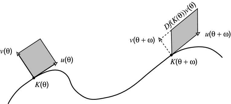
Figure 2. Illustration of the geometric reason for reducibility of the equations in the center. Note that the base of a rectangle gets mapped into the base of the other (differentiating the invariance). The preservation of the symplectic form implies that the symplectic area of both rectangles is the same.

The matrix $\tilde{M}(\theta)$ is not invertible since it is not square. However we can derive a generalized inverse for $\tilde{M}(\theta)$. As a motivation for subsequent developments, we first present Lemma 4.12 which deals with the geometric cancellations in the case of an exactly invariant torus. The case of interest for a KAM algorithm — when the torus is only approximately invariant — will be studied in Lemma 4.14 as a perturbation of Lemma 4.12.

A straightforward calculation shows that

(47) $$\tilde{M}^{\top}J^{c}(K)\tilde{M}=\begin{pmatrix}\hat{L}&{\rm Id}_{l}\\ -{\rm Id}_{l}&(N^{\top}DK^{\top}J^{c}(K)^{-\top}DK\,N\end{pmatrix}.$$

Lemma 4.12.

Let $K$ be a solution of (11). Then the matrix $\tilde{M}^{\top}J^{c}(K)\tilde{M}$ is invertible and

$$(\tilde{M}^{\top}J^{c}(K)\tilde{M})^{-1}=\begin{pmatrix}(-N^{\top}DK^{\top}J^{c}(K)^{-\top}DK\,N&-{\rm Id}_{l}\\ {\rm Id}_{l}&0\end{pmatrix}.$$

Proof.

It follows immediately from (47) and the isotropic character of the invariant torus, i.e. $\hat{L}=0$. ∎

Now we consider the case we are interested in, that is when $K$ is an approximate solution with an error $E(\theta)=\mathcal{F}_{\omega}(\lambda,K)(\theta)$, assumed to be small. We will need the invertibility of $\tilde{M}(\theta)^{\top}J^{c}(K(\theta))\tilde{M}(\theta)$ in this case.

More precisely, we introduce

(48) $$e(\theta)=DF_{\lambda}(K(\theta))\tilde{M}(\theta)-\tilde{M}(\theta+\omega)\mathcal{S}_{\lambda}(\theta),$$

where $\mathcal{S}_{\lambda}$ is given by (43). If we denote $e(\theta)=(e_{1}(\theta),e_{2}(\theta))$, a simple algebraic computation yields

$$\begin{split}&e_{1}(\theta)=DE^{c}(\theta)\\ &e_{2}(\theta)=[(DF_{\lambda}J^{c}(K)^{-1}DK\,N](\theta)-DK(\theta+\omega)A_{\lambda}(\theta)\\ &-[J^{c}(K)^{-1}DK\,N](\theta+\omega)=O(E,DE)\end{split}$$

by the choice of $A_{\lambda}$.

We first prove the approximate isotropic character of the torus

Lemma 4.13.

Under the previous conditions, let $K\in{\mathcal{A}}_{\rho,\underline{c},\Gamma}$ be a function which solves (11) approximately and let $E=F_{\lambda}\circ K-K\circ T_{\omega}$ be the corresponding error. Then for $0<\delta<\rho/2$,

(49) $$\|L\|_{\rho-2\delta,\Gamma}\leq C\kappa\,\delta^{-(\nu+1)}\ \|E\|_{\rho,\underline{c},\Gamma},$$

where $C$ depends on $l,\nu,R,\rho,\ \|DK\|_{\rho,\underline{c},\Gamma},\|F_{\lambda}\|_{C^{1}_{\Gamma}(B_{r})},\|J^{c}(K)\|_{C^{1}(B_{r})}$.

Proof.

We define the two-form on the torus ${\mathbb{T}}^{l}$

$$\Omega_{e}=K^{*}\Omega_{\infty}-(K\circ T_{\omega})^{*}\Omega_{\infty}.$$

The corresponding matrix is $L-L\circ T_{\omega}$. Using that $F_{\lambda}$ is symplectic we have that for any $(\xi,\eta)\in{\mathbb{R}}^{2l}$

$$\Omega_{e}(\theta)(\xi,\eta) =\big{(}(F_{\lambda}\circ K)^{*}\Omega_{\infty}-(K\circ T_{\omega})^{*}\Omega_{\infty}\big{)}(\theta)(\xi,\eta)$$

$$=\displaystyle\sum_{i\in{\mathbb{Z}}^{N}}\Big{[}\Omega\Big{(}(F_{\lambda})_{i}\big{(}K(\theta)\big{)}\Big{)}\big{(}D((F_{\lambda})_{i}\circ K)(\theta)\xi,\ D((F_{\lambda})_{i}\circ K)(\theta)\eta\big{)}$$

$$\quad-\Omega\big{(}K\circ T_{\omega}(\theta)\big{)}\big{(}D(K_{i}\circ T_{\omega})(\theta)\xi,\ D(K_{i}\circ T_{\omega})(\theta)\eta\big{)}\Big{]}.$$

Since $D((F_{\lambda})_{i}\circ K)-D(K_{i}\circ T_{\omega})=DE_{i}$ and $\|DE\|_{\rho-\delta,\underline{c},\Gamma}\leq\frac{1}{\delta}\,\|E\|_{\rho,\underline{c},\Gamma}$, using the decay properties of $F\circ K$ and $K\circ T_{\omega}$ to sum the series, we obtain that

(50) $$L-L\circ T_{\omega}=g$$

with $\|g\|_{\rho-\delta}\leq C\delta^{-1}\,\|E\|_{\rho,\underline{c},\Gamma}$ for some $C$ as in the statement. Now we use Proposition 4.4 to finish the proof. ∎

The next step is to ensure the invertibility of the $2l\times 2l$-matrix $\tilde{M}^{\top}J^{c}(K)\tilde{M}$. According to expression (47), we can write

$$\tilde{M}(\theta)^{\top}J^{c}(K)\tilde{M}(\theta)=V(\theta)+R(\theta),$$

where

$$V=\begin{pmatrix}0&{\rm Id}_{l}\\ -{\rm Id}_{l}&N^{\top}DK^{\top}J^{c}(K)^{-\top}DK\,N\end{pmatrix}$$

and

$$R=\begin{pmatrix}\hat{L}&0\\ 0&0\end{pmatrix}.$$

We have the following lemma, providing the desired invertibility result under a smallness assumption on $E$, namely (51) in the next lemma.

Lemma 4.14.

There exists a constant $C>0$ such that if

(51) $$C\kappa\delta^{-(\nu+1)}\|E\|_{\rho,\underline{c},\Gamma}\leq 1/2$$

for some $0<\delta<\rho/2$ then the matrix $\tilde{M}^{\top}(\theta)J^{c}(K)\tilde{M}(\theta)$ is invertible for $\theta\in D_{\rho-2\delta}$ and there exists a matrix $\tilde{V}(\theta)$ such that

$$(\tilde{M}(\theta)^{\top}J^{c}(K(\theta))\tilde{M}(\theta))^{-1}=V(\theta)^{-1}+\tilde{V}(\theta)$$

with

$$\tilde{V}(\theta)=\Big{(}\sum_{k=1}^{\infty}(-1)^{k}(V(\theta)^{-1}R(\theta))^{k}\Big{)}V(\theta)^{-1},$$

where the series is absolutely convergent. Furthermore, we have the estimate

(52) $$\|\tilde{V}\|_{\rho-2\delta,\Gamma}\leq C^{\prime}\kappa\delta^{-(\nu+1)}\|E\|_{\rho,\underline{c},\Gamma},$$

where the constant $C^{\prime}>0$ depends on $l$, $\nu$, $\|F_{/}\textlnot ambda\|_{C_{\Gamma}^{1}(B_{r})}$, $\|J^{c}(K)\|_{C_{\Gamma}^{1}(B_{r})}$, $\|DK\|_{\rho,\underline{c},\Gamma}$, $\|N\|_{\rho,\Gamma}$.

Proof.

The matrix $V(\theta)$ is invertible with

$$V^{-1}=\begin{pmatrix}N^{\top}DK^{\top}J^{c}(K)^{-\top}DK\,N&-{\rm Id}_{l}\\ {\rm Id}_{l}&0\end{pmatrix}.$$

We can write

$$\tilde{M}(\theta)^{\top}J^{c}(K(\theta))\tilde{M}(\theta)=V(\theta)({\rm Id}_{2l}+V(\theta)^{-1}R(\theta)).$$

To apply the Neumann series (and consequently justify the existence of the inverse of ${\rm Id}_{2l}+V^{-1}R$ as well as the estimates for its size), we have to estimate the term $V^{-1}R$. According to Lemma 4.13, we have the estimate for $L$

$$\|L\|_{\rho-2\delta,\Gamma}\leq C\kappa\delta^{-(\nu+1)}\|E\|_{\rho,\underline{c},\Gamma}$$

for all $\delta\in(0,\rho/2)$. This leads to the estimate

$$\|V^{-1}R\|_{\rho-2\delta,\Gamma}\leq C\kappa\delta^{-(\nu+1)}\|E\|_{\rho,\underline{c},\Gamma}$$

for $0<\delta<\rho/2$, where $C>0$ depends on $l$, $\nu$, $\|DK\|_{\rho,\underline{c},\Gamma}$, $\|N\|_{\rho,\Gamma}$ and $\|J^{c}(K)^{c}\|_{\rho,\Gamma}$. Because of assumption (51), we have that the right-hand side of the last equation is less than $1/2$.

Then the matrix ${\rm Id}_{2l}+V(\theta)^{-1}R(\theta)$ is invertible with

$$\|({\rm Id}_{2l}+V^{-1}R)^{-1}\|_{\rho-2\delta,\Gamma}\leq\frac{1}{1-\|V^{-1}R\|_{\rho-2\delta,\Gamma}}\leq 2.$$

Now the estimates follow immediately. ∎

4.3.5. Identification of the center subspace

In this section, we identify the center space as being very close (up to terms that can be bounded by the error) to the range of the matrix $\tilde{M}$. This will allow us to use the range of $\tilde{M}$ in place of ${\mathcal{E}}_{K(\theta)}^{c}$ without changing the quadratic character of the method.

Proposition 4.15.

Denote by $\Gamma_{K(\theta)}$ the range of $\tilde{M}(\theta)$ and by $\Pi^{\Gamma}_{K(\theta)}$ the projection onto $\Gamma_{K(\theta)}$ according to the splitting ${\mathcal{E}}^{s}_{K(\theta)}\oplus\Gamma_{K(\theta)}\oplus{\mathcal{E}}^{u}_{K(\theta)}$.

Then there exists a constant $C>0$ such that if

$$\delta^{-1}\|E\|_{\rho,\underline{c},\Gamma}\leq C$$

we have the estimate

(53) $$\|\Pi_{K(\theta)}^{c}-\Pi_{K(\theta)}^{\Gamma}\|_{\rho-2\delta,\underline{c},\Gamma}\leq C\delta^{-1}\|E\|_{\rho,\underline{c},\Gamma}$$

for every $\delta\in(0,\rho/2)$ and where $C$, as usual, depends on the non-degeneracy constants of the problem.

Proof.

From (48) and Cauchy estimates (see Lemma A.8 in Appendix A), we have:

$${\rm dist}_{\rho-\delta,\underline{c},\Gamma}((DF_{\lambda}\circ K)\Gamma_{K(\theta)},\Gamma_{K(\theta)}\circ T_{\omega})\leq C\delta^{-1}\|E\|_{\rho,\underline{c},\Gamma},$$

where $dist$ stands for the distance between two spaces at the Grassmannian level. Using again equation (48) and iterating it, we obtain for $n\geq 1$

$$DF_{\lambda}(K(\theta+n\omega))\times\cdots\times DF_{\lambda}(K(\theta))\tilde{M}(\theta)=$$

$$\tilde{M}(\theta+n\omega){\mathcal{S}}_{\lambda}(\theta+(n-1)\omega)\times\cdots\times{\mathcal{S}}_{\lambda}(\theta)+R_{n},$$

where

$$\|R_{n}\|_{\rho-\delta,\underline{c},\Gamma}\leq C_{n}\delta^{-1}\|E\|_{\rho,\underline{c},\Gamma}$$

and $C_{n}$ depends on $n$.

Since ${\mathcal{S}}_{\lambda}(\theta)$ is upper triangular with Id_l on the diagonal, we have:

$${\mathcal{S}}_{\lambda}(\theta+(n-1)\omega)\times\cdots\times{\mathcal{S}}_{\lambda}(\theta)=\begin{pmatrix}&{\rm Id}_{l}&A_{\lambda}(\theta+(n-1)\omega)+\cdots+A_{\lambda}(\theta)\\ &0&{\rm Id}_{l}\end{pmatrix}.$$

Therefore, by induction, we have for every $n\in{\mathbb{N}}$

$$\|DF_{\lambda}(K(\theta+n\omega))\cdots DF_{\lambda}(K(\theta))\tilde{M}(\theta)\|_{\rho-\delta,\underline{c},\Gamma}\leq Cn+C_{n}\delta^{-1}\|E\|_{\rho,\underline{c},\Gamma}.$$

Identical calculations give that

$$\|DF_{\lambda}^{-1}(K(\theta-n\omega))\cdots DF_{\lambda}^{-1}(K(\theta))\tilde{M}(\theta+\omega)\|_{\rho-\delta,\underline{c},\Gamma}\leq Cn+C_{n}\delta^{-1}\|E\|_{\rho,\underline{c},\Gamma}.$$

Note that, given any $\mu_{3}>1$ (as in Definition 3.1), there exists an integer $n_{\mu_{3}}\geq 0$ such that for all $n\geq n_{\mu_{3}}$, we have $Cn<\mu_{3}^{n}$. Consequently, choosing such $n_{\mu_{3}}$ there exists a constant $C$ such that if the error satisfies

$$\delta^{-1}\|E\|_{\rho,\underline{c},\Gamma}\leq C,$$

we have $Cn+C_{n}\delta^{-1}\|E\|_{\rho,\underline{c},\Gamma}<\mu_{3}^{n}$. In other words, the above estimates hold for all sufficiently large $n$, provided that we impose a suitable smallness condition on $\delta^{-1}\|E\|_{\rho,\underline{c},\Gamma}$.

As a consequence, $\Gamma_{K(\theta)}$ is an approximately invariant bundle, and we also have bounds on the rate of growth of the co-cycle both in positive and negative times. Using Proposition 4.2, this shows that indeed one can find a true invariant subspace $\tilde{\mathcal{E}}_{K(\theta)}$ close to $\Gamma_{K(\theta)}$. Since this invariant subspace should be of the same dimension of the center space ${\mathcal{E}}^{c}_{K(\theta)}$, we deduce that

$$\tilde{\mathcal{E}}_{K(\theta)}={\mathcal{E}}^{c}_{K(\theta)}.$$

∎

4.3.6. Estimates on the center subspace

We recall the projection into the center subspace of the linearized equation

(54) $$\Pi^{c}_{K(\theta+\omega)}\frac{\partial F_{\lambda}}{\partial\lambda}(K(\theta))\Lambda+DF_{\lambda}(K(\theta))\Delta^{c}(\theta)-\Delta^{c}(\theta+\omega)=-E^{c}(\theta).$$

To shorten the notation till the end of the section we will write$\frac{\partial F_{\lambda}}{\partial\lambda}$ $(K(\theta))\Lambda$ instead of $\Pi^{c}_{K(\theta+\omega)}\frac{\partial F_{\lambda}}{\partial\lambda}(K(\theta))\Lambda$.

We introduce the new function $W(\theta)$ through

(55) $$\Delta^{c}(\theta)=\tilde{M}(\theta)W(\theta)+\hat{e}(\theta)W(\theta),$$

where

(56) $$\hat{e}=\Pi_{K(\theta+\omega)}^{c}-\Pi_{K(\theta+\omega)}^{\Gamma}$$

which was estimated in Proposition 4.15.

Substituting (55) into equation (54) we get

(57) $$DF(K(\theta))\tilde{M}(\theta)W(\theta)-\tilde{M}(\theta+\omega)W(\theta+\omega)$$

$$=-E^{c}(\theta)-\frac{\partial F_{\lambda}}{\partial\lambda}(K(\theta))\Lambda+\hat{e}(\theta+\omega)W(\theta+\omega)-DF(K(\theta))\hat{e}(\theta)W(\theta)$$

We anticipate that the term $\hat{e}W$ will be quadratic in the error. Similarly, writing

$$\frac{\partial F_{\lambda}}{\partial\lambda}(K(\theta))=\Pi^{\Gamma}_{K(\theta+\omega)}\frac{\partial F_{\lambda}}{\partial\lambda}(K(\theta))+\hat{e}\frac{\partial F_{\lambda}}{\partial\lambda}(K(\theta)).$$

we also anticipate that the term $\hat{e}\frac{\partial F_{\lambda}}{\partial\lambda}(K(\theta))\Lambda$ will be quadratic in the error. As a consequence, we will ignore these two terms and the equation for $W$ is

(58) $$DF_{\lambda}(K(\theta))\tilde{M}(\theta)W(\theta)-\tilde{M}(\theta+\omega)W(\theta+\omega)=-E^{c}(\theta)-\frac{\partial F_{\lambda}}{\partial\lambda}(K(\theta))\Lambda.$$

Using $e(\theta)$ above and multiplying equation (58) by $\tilde{M}(\theta+\omega)^{\top}J^{c}(K(\theta+\omega))$, using Lemma 4.14 (giving the invertibility of $\tilde{M}^{\top}J^{c}(K)\tilde{M}$) and equation (48), we end up with

(59) $$\left[\begin{pmatrix}{\rm Id}_{l}&A_{\lambda}(\theta)\\ 0_{l}&{\rm Id}_{l}\end{pmatrix}+B(\theta)\right]W(\theta)-W(\theta+\omega)=p_{1}(\theta)+p_{2}(\theta)$$

$$-[\tilde{M}^{\top}J^{c}(K)\tilde{M}](\theta+\omega)^{-1}[\tilde{M}^{\top}J^{c}(K)](\theta+\omega)\frac{\partial F_{\lambda}}{\partial\lambda}(K(\theta))\Lambda,$$

where

(60) $$B(\theta)=[\tilde{M}^{\top}J^{c}(K)\tilde{M}](\theta+\omega)^{-1}[\tilde{M}^{\top}J^{c}(K)](\theta+\omega)e(\theta),$$

(61) $$p_{1}(\theta)=-V(\theta+\omega)^{-1}[\tilde{M}^{\top}J^{c}(K)](\theta+\omega)E^{c}(\theta)$$

and

(62) $$p_{2}(\theta)=-\tilde{V}(\theta+\omega)[\tilde{M}^{\top}J^{c}(K)](\theta+\omega)E^{c}(\theta).$$

The next result provides the estimates of the previously introduced quantities.

Lemma 4.16.

Assume $\omega\in D(\kappa,\nu)$ and $\delta$ and $\|E\|_{\rho,\underline{c},\Gamma}$ satisfy (51). Then using the linear change of variables (55), equation (58) becomes

$$\begin{split}&\left[{\mathcal{S}}_{\lambda}(\theta)+B(\theta)\right]W(\theta)-W(\theta+\omega)=p_{1}(\theta)+p_{2}(\theta)\\ &-[\tilde{M}^{\top}J^{c}(K)\tilde{M}](\theta+\omega)^{-1}[\tilde{M}^{\top}J^{c}(K)](\theta+\omega)\frac{\partial F_{\lambda}}{\partial\lambda}(K(\theta))\Lambda,\end{split}$$

where $B$, $p_{1}$ and $p_{2}$ are given by equations (60), (61) and (62) respectively.

Moreover the following estimates hold: for $p_{1}$ we have

(63) $$\|p_{1}\|_{\rho,\underline{c},\Gamma}\leq C\|E\|_{\rho,\underline{c},\Gamma},$$

where $C$ only depends on $\|J^{c}(K)\|_{\rho,\Gamma}$, $\|N\|_{\rho}$, $\|DK\|_{\rho,\underline{c},\Gamma}$. For $p_{2}$ and $B$, we have

(64) $$\|p_{2}\|_{\rho-2\delta,\underline{c},\Gamma}\leq C\kappa\delta^{-(\nu+1)}\|E\|^{2}_{\rho,\underline{c},\Gamma}$$

and

(65) $$\|B\|_{\rho-2\delta,\Gamma}\leq C\delta^{-1}\|E\|_{\rho,\underline{c},\Gamma},$$

where $C$ depends $l$, $\nu$, $\rho$, $R$, $\|N\|_{\rho}$, $\|DK\|_{\rho,\underline{c},\Gamma}$, $\|F_{\lambda}\|_{C_{\Gamma}^{1}(B_{r})}$, $\|J^{c}(K)\|_{C^{1}(B_{r})}$.

Proof.

We have basically to estimate $\tilde{M}(\theta+\omega)^{\top}J^{c}(K(\theta+\omega))E^{c}(\theta)$ and $\tilde{M}(\theta+\omega)^{\top}J^{c}(K(\theta+\omega))e(\theta)$ and then use Lemma 4.14. First we bound

$$|E^{c}_{i}(\theta)| \leq\sum_{j\in{\mathbb{Z}}^{N}}\,|(\Pi^{c}_{K(\theta+\omega)})_{ij}|\ |E_{j}(\theta)|$$

$$\leq\sum_{j\in{\mathbb{Z}}^{N}}\,\|\Pi^{c}_{K(\theta+\omega)}\|_{\rho,\Gamma}\ \Gamma(i-j)\ \|E\|_{\rho,\underline{c},\Gamma}\ \max_{k}\ \Gamma(j-c_{k})$$

$$\leq\|\Pi^{c}_{K(\theta+\omega)}\|_{\rho,\Gamma}\ \|E\|_{\rho,\underline{c},\Gamma}\ \sum^{R}_{k=1}\Gamma(i-c_{k})\,.$$

For $1\leq i\leq l$ we have, taking into account that $J^{c}$ is uncoupled,

(66) $$|\big{(}\tilde{M}(\theta+\omega)^{\top}\,J^{c}(K)E^{c}(\theta)\big{)}_{i}|\leq C\sum_{j\in{\mathbb{Z}}^{N}}\,|\partial_{\theta_{i}}\,K_{j}(\theta+\omega)|\,\,|E^{c}_{j}(\theta)|.$$

We estimate from above by

(67) $$\begin{split}\sum_{j\in{\mathbb{Z}}^{N}}\,&|D_{\theta_{i}}\,K_{j}(\theta+\omega)|\ |E^{c}_{j}(\theta)|\\ &\leq\sum_{j}\,\|DK\|_{\rho,\underline{c},\Gamma}\ \max_{m}\,\Gamma(j-c_{m})\,\|\Pi^{c}_{K(\theta+\omega)}\|_{\rho,\Gamma}\,\|E\|_{\rho,\underline{c},\Gamma}\,\sum^{R}_{k=1}\Gamma(j-c_{k})\\ &\leq R\,\|DK\|_{\rho,\underline{c},\Gamma}\ \|\Pi^{c}_{K(\theta+\omega)}\|_{\rho,\Gamma}\,\|E\|_{\rho,\underline{c},\Gamma}\,.\end{split}$$

For $l+1\leq i\leq 2l$, one gets

(68) $$|\big{(}\tilde{M}(\theta+\omega)^{\top}J^{c}(K(\theta))\,E^{c}(\theta)\big{)}_{i}|\leq$$

$$C|\Big{(}N(\theta+\omega)^{\top}DK(\theta+\omega)^{\top}\,\tilde{J}^{c}\big{(}K(\theta+\omega)^{\top}\big{)}\,E^{c}(\theta)\Big{)}_{i}|.$$

We get a similar bound for (68) taking into account that $N$ is a bounded finite dimensional matrix. Now the bounds (63) and (64) follow immediately from Lemma 4.14. For the estimate on $B$ we use Cauchy estimates for $e_{1}(\theta)$. From

$$B(\theta)=(V(\theta+\omega)^{-1}+\tilde{V}(\theta+\omega))\tilde{M}(\theta+\omega)^{\top}e(\theta)$$

we have

$$\begin{split}\|B\|_{\rho-2\delta}&\leq\|V(\theta+\omega)^{-1}\|_{\rho-2\delta}\|\tilde{M}(\theta+\omega)^{\top}e(\theta)\|_{\rho-2\delta}\\ &\quad+\ |\tilde{V}(\theta+\omega)\tilde{M}(\theta+\omega)^{\top}e(\theta)\|_{\rho-2\delta}\end{split}$$

and using estimate (52) we end up with

$$\|B\|_{\rho-2\delta,\Gamma}\leq C\delta^{-1}\|E\|_{\rho,\underline{c},\Gamma}+\kappa\delta^{-(\nu+1)}\|E\|_{\rho,\underline{c},\Gamma}\ \delta^{-1}\|E\|_{\rho,\underline{c},\Gamma}.$$

This gives the desired result. ∎

4.3.7. Approximate solvability of the linearized equation on the center subspace

In this section we find a solution of equation (59) up to quadratic error. The convergence of the Newton scheme is of course not affected (see [Zeh75]).

For that we introduce the following operator

$${\mathcal{L}}W(\theta)=\begin{pmatrix}{\rm Id}_{l}&A_{\lambda}(\theta)\\ 0_{l}&{\rm Id}_{l}\end{pmatrix}W(\theta)-W(\theta+\omega).$$

Then equation (59) can be written as

(69) $${\mathcal{L}}W(\theta) +B(\theta)W(\theta)=p_{1}(\theta)+p_{2}(\theta)$$

$$-[\tilde{M}^{\top}J^{c}(K)\tilde{M}](\theta+\omega)^{-1}[\tilde{M}^{\top}J^{c}(K)](\theta+\omega)\frac{\partial F_{\lambda}}{\partial\lambda}(K(\theta))\Lambda.$$

We will reduce equation (69) to two small divisors equations. Generically their right-hand sides will not have zero average, but we will use the freedom in choosing $\Lambda$ and in fixing the average of the solution to solve one after the other. By Lemma 4.14 we can write

$$[(\tilde{M}^{\top}J^{c}(K)\tilde{M})^{-1}\tilde{M}^{\top}J^{c}(K)](\theta+\omega)\frac{\partial F_{\lambda}(K(\theta))}{\partial\lambda}\Lambda=H(\theta)\Lambda+q(\theta)\Lambda,$$

where the $2l\times l$ matrix $H$ is

$$H(\theta)=V(\theta+\omega)^{-1}\tilde{M}(\theta+\omega)^{\top}J^{c}(K(\theta+\omega))\frac{\partial F_{\lambda}(K(\theta))}{\partial\lambda}$$

and $q$ satisfies for all $\delta\in(0,\rho/2)$

$$\|q\|_{\rho-2\delta,\Gamma}\leq C\kappa\delta^{-(\nu+1)}\Big{\|}\frac{\partial F_{\lambda}(K(\theta))}{\partial\lambda}\Big{\|}_{\rho,\underline{c},\Gamma}\,\|E\|_{\rho,\underline{c},\Gamma},$$

where the constant $C$ depends on $l$, $\nu$, $\rho$, $R$, $\|N\|_{\rho}$, $\|DK\|_{\rho,\underline{c},\Gamma}$, $\|F\|_{C_{\Gamma}^{1}(B_{r})}$, $\|J^{c}(K)\|_{C^{1}(B_{r})}$.

We will take as an approximate solution the solution $v$ of

(70) $${\mathcal{L}}v(\theta)=p_{1}(\theta)-H(\theta)\Lambda$$

obtained from (69) by removing the terms containing $B,p_{2}$ and $q$.

Proposition 4.17.

Assume $\omega\in D(\kappa,\nu)$ and $(\lambda,K)$ is a non-degenerate pair (i.e. $(\lambda,K)\in ND_{loc}(\rho,\Gamma)$). If the error $\|E\|_{\rho,\underline{c},\Gamma}$ satisfies (51), there exist a mapping $v\in\mathcal{A}_{\rho-2\delta,\underline{c},\Gamma}$ for any $0<\delta<\rho/2$ and a vector $\Lambda\in\mathbb{R}^{l}$ solving equation (70).

Moreover there exists a constant $C>0$ depending on $\nu,\rho,l,R,\|K\|_{\rho,\underline{c},\Gamma},$ $|{\rm avg\,}(Q_{\lambda})|^{-1}$, $|{\rm avg\,}(A_{\lambda})|^{-1}$, $\|N\|_{\rho}$ and $\|J^{c}(K)\|_{\rho}$ such that

(71) $$\|v\|_{\rho-2\delta,\underline{c},\Gamma}<C\kappa^{2}\delta^{-2\nu}\|E\|_{\rho,\underline{c},\Gamma}$$

and

$$|\Lambda|<C\|E\|_{\rho,\underline{c},\Gamma}.$$

Proof.

We denote $T(\theta)$ the right-hand side of equation (70), i.e. we have to solve

(72) $${\mathcal{L}}v(\theta)=T(\theta),$$

with

$$T=p_{1}-H\Lambda.$$

We now decompose equation (72) into two equations. Writing $v=(v_{1},v_{2})^{\top}$, $T(\theta)=(T_{1}(\theta),T_{2}(\theta))^{\top}$ equation (72) is equivalent to

(73) $$v_{1}(\theta)+A_{\lambda}(\theta)v_{2}(\theta)=v_{1}(\theta+\omega)+T_{1}(\theta),$$

(74) $$v_{2}(\theta)=v_{2}(\theta+\omega)+T_{2}(\theta).$$

A simple computation shows that

$$T_{2}(\theta)=-[DK^{\top}J^{c}(K)]\circ T_{\omega}\circ(E_{2}^{c}+\frac{\partial F_{\lambda}(K(\theta))}{\partial\lambda}\Lambda)$$

We begin by solving equation (74). To apply Proposition 4.4 we choose $\Lambda\in{\mathbb{R}}^{l}$ such that

$${\rm avg\,}(T_{2})=0.$$

This condition is equivalent to

$${\rm avg\,}\Big{(}DK^{\top}(\omega+\theta)J^{c}(K(\omega+\theta))(E^{c}(\theta)+\frac{\partial F_{\lambda}(K(\theta))}{\partial\lambda}\Lambda)\Big{)}=0.$$

This leads to

$${\rm avg\,}\Big{(}(DK^{\top}(\omega+\theta) J^{c}(K(\omega+\theta))\frac{\partial F_{\lambda}(K(\theta))}{\partial\lambda}\Big{)}\Lambda$$

$$= -{\rm avg\,}\Big{(}DK^{\top}(\omega+\theta)J^{c}(K(\omega+\theta))E^{c}(\theta)\Big{)}.$$

Note that the matrix which applies to $\Lambda$ is the average of $Q_{\lambda}$ which, by hypothesis, is invertible. This gives $|\Lambda|<C\,\|E\|_{\rho,\underline{c},\Gamma}$.

From the expression of $T$ and the value of $\Lambda$ obtained above, we have that there exists a constant $C$ such that

$$\|T_{i}\|_{\rho,\underline{c},\Gamma}\leq C\|E\|_{\rho,\underline{c},\Gamma},$$

for $i=1,2$.

Then Proposition 4.4 provides us with an analytic solution $v_{2}$ on $D_{\rho-\delta}$ with arbitrary average and

(75) $$\|v_{2}\|_{\rho-\delta,\underline{c},\Gamma}\leq C\kappa\delta^{-\nu}\|T_{2}\|_{\rho,\underline{c},\Gamma}+|{\rm avg\,}(v_{2})|.$$

Now we come to equation (73). To apply Proposition 4.4 we choose ${\rm avg\,}(v_{2})$ such that ${\rm avg\,}(T_{1}-A_{\lambda}v_{2})=0$. This condition is equivalent to

$${\rm avg\,}(v_{2})={\rm avg\,}(A_{\lambda})^{-1}({\rm avg\,}(T_{1})-{\rm avg\,}(A_{\lambda}v^{\perp}_{2})),$$

where $v_{2}=v_{2}^{\perp}+{\rm avg\,}(v_{2})$. This is possible since by the twist condition ${\rm avg\,}(A_{\lambda})$ is invertible.

We have that

$$|{\rm avg\,}(v_{2})|\leq C\kappa\delta^{-\nu}\,\|E\|_{\rho,\underline{c},\Gamma}.$$

Then we take $v_{1}$ as the unique analytic solution of (73) with zero average. Furthermore, we have the estimate

$$\|v_{1}\|_{\rho-2\delta,\underline{c},\Gamma}\leq C\kappa\delta^{-\nu}\|T_{1}-A_{\lambda}v_{2}\|_{\rho-\delta,\underline{c},\Gamma}.$$

Collecting the previous bounds we get the result. ∎

We now come back to the solutions of (38). The above procedure allows us to prove the following proposition, providing an approximate solution of the projection of $D_{\lambda,K}\mathcal{F}_{\omega}(\lambda,K)(\Lambda,\Delta)=-E$ on the center subspace.

Proposition 4.18.

Let $(\Lambda,W)$ be as in Proposition 4.17 and assume the hypotheses of that proposition hold. Define $\Delta^{c}(\theta)=\tilde{M}(\theta)W(\theta)$. Then, equation (38) is approximately solvable and we have the following estimates

(76) $$\|\Delta^{c}\|_{\rho-2\delta,\underline{c},\Gamma}\leq C\kappa^{2}\delta^{-2\nu}\|E\|_{\rho,\underline{c},\Gamma},$$

$$\quad|\Lambda|\leq C\|E\|_{\rho,\underline{c},\Gamma},$$

where the constant $C$ depends on $\nu,\rho,l,R,|{\rm avg\,}(Q_{\lambda})|^{-1}$, $|{\rm avg\,}(A_{\lambda})|^{-1}$, $\|N\|_{\rho}$, $\|\frac{\partial F_{\lambda}(K)}{\partial\lambda}\|_{\rho,\underline{c},\Gamma}$ and $\|J^{c}(K)\|_{\rho}$ and

(77) $$\|D_{\lambda,K}\mathcal{F}_{\omega}(\lambda,K)(\Lambda,\Delta^{c})+E^{c}\|_{\rho-2\delta,\underline{c},\Gamma}\leq C\kappa^{2}\delta^{-(2\nu+1)}(\|E\|^{2}_{\rho,\underline{c},\Gamma}+\|E\|_{\rho,\underline{c},\Gamma}|\Lambda|),$$

where the constant $C$ depends on $l$, $\nu$, $\rho$, $R$, $\|F\|_{C_{\Gamma}^{1}(B_{r})}$, $\|DK\|_{\rho,\underline{c},\Gamma}$, $\|N\|_{\rho}$, $|{\rm avg\,}(A_{\lambda})|^{-1}$, $|{\rm avg\,}(Q_{\lambda})|^{-1}$ and $\|\frac{\partial F_{\lambda}(K)}{\partial\lambda}\|_{\rho,\underline{c},\Gamma}$.

Proof.

For the first estimate we take $\theta\in D_{\rho-2\delta}$ and write $W=(W_{1},W_{2})$. Then

$$\Delta^{c}(\theta)=DK(\theta)W_{1}(\theta)+J^{c}(K(\theta))^{-1}DK(\theta)N(\theta)W_{2}(\theta).$$

We have

$$\begin{split}\big{|}(DK(\theta)W_{1}(\theta))_{i}\big{|}&=\Big{|}\sum^{l}_{j=1}D_{\theta_{j}}K_{i}(\theta)W_{1,j}(\theta)\Big{|}\\ &\leq\|DK\|_{\rho,\underline{c},\Gamma}\,\max_{k}\,\Gamma(i-c_{k})\|W_{1}\|_{\rho-2\delta}.\end{split}$$

Also, since $J_{\infty}$ is uncoupled and $N$ is finite dimensional,

$$\begin{split}&\Big{|}\big{(}J^{c}(K(\theta))^{-1}DK(\theta)N(\theta)W_{2}(\theta)\big{)}_{i}\Big{|}\leq\|J(K)\|_{\rho}\Big{|}\big{(}DK(\theta)N(\theta)W_{2}(\theta)\big{)}_{i}\Big{|}\\ &\qquad\leq\|J(K)\|_{\rho}\|N\|_{\rho}\|DK\|_{\rho,\underline{c},\Gamma}\,\max\,\Gamma(i-c_{k})\|W_{2}\|_{\rho-2\delta}.\end{split}$$

Now using (71), we obtain (76).

For (77), using the previous notations and Lemma 4.16,

(78) $$\begin{split}D_{\lambda,k}\,&{\mathcal{F}}_{\omega}(\lambda,K)(\Lambda,\Delta_{c})(\theta)+E^{c}(\theta)\\ &=\frac{\partial F_{\lambda}}{\partial\lambda}(K(\theta))\Lambda+\tilde{M}(\theta+\omega)\big{[}{\mathcal{S}}_{\lambda}(\theta)W(\theta)-W(\theta+\omega)\big{]}\\ &\quad+e(\theta)W(\theta)+E^{c}(\theta)=\frac{\partial F_{\lambda}}{\partial\lambda}(K(\theta))\Lambda\\ &\quad+\tilde{M}(\theta+\omega)\big{[}p_{1}(\theta)-Q(\theta)\Lambda\big{]}+e(\theta)W(\theta)+E^{c}(\theta).\end{split}$$

Note that

$$\tilde{M}(\theta+\omega)p_{1}(\theta)=$$

$$\tilde{M}(\theta+\omega)\big{[}-([\tilde{M}^{\top}J^{c}(K)\tilde{M})^{-1}](\theta+\omega)[\tilde{M}^{\top}J^{c}(K)](\theta+\omega)E^{c}(\theta)-p_{2}(\theta)\big{]}$$

and also that $\tilde{M}(\tilde{M}^{\top}J^{c}(K)\tilde{M})^{-1}\tilde{M}^{\top}J^{c}(K)$ is symmetric and

$$\tilde{M}\tilde{M}^{\top}J^{c}(K)\tilde{M})^{-1}\tilde{M}^{\top}J^{c}(K)-{\rm Id}$$

maps the vectors of the center subspace to zero because it is generated by the columns of $\tilde{M}$.

Also we have

$$\tilde{M}(\theta+\omega)Q_{\lambda}(\theta)\Lambda=$$

$$\tilde{M}(\theta+\omega)\Big{[}[\tilde{M}^{\top}J^{c}(K)\tilde{M})^{-1}\tilde{M}^{\top}J^{c}(K)](\theta+\omega)\frac{\partial F_{\lambda}}{\partial\lambda}(K(\theta))\Lambda-q(\theta)\Lambda\Big{]}.$$

We recall that here the derivative of $F_{\lambda}$ with respect to $\lambda$ actually means the projection of it into the center subspace.

Therefore (78) becomes

$$\tilde{M}(\theta+\omega)[q(\theta)\Lambda-p_{2}(\theta)]+e(\theta)W(\theta)$$

and (77) follows. ∎

4.4. Solution of the equation in the hyperbolic subspaces

In this section, we study the projection of the Newton equation (27) on the the hyperbolic spaces.

According to the splitting (12), there exist projections on the linear spaces $\mathcal{E}^{s}_{{K(\theta)}}$ and $\mathcal{E}^{u}_{{K(\theta)}}$. The analytic regularity of the splitting implies the analytic dependence of these projections in $\theta$. We denote $\Pi^{s}_{K(\theta)}$ (resp. $\Pi^{u}_{K(\theta)}$) the projections on the stable (resp. unstable) invariant subspace.

We project equation (27) on the stable and unstable subspaces to obtain

(79) $$\Pi^{s}_{K(\theta+\omega)}\Big{(}\frac{\partial F_{\lambda}(K(\theta))}{\partial\lambda}\Lambda+DF_{\lambda}(K(\theta))\Delta(\theta)-\Delta(\theta+\omega)\Big{)}=-\Pi^{s}_{K(\theta+\omega)}E(\theta),$$

(80) $$\Pi^{u}_{K(\theta+\omega)}\Big{(}\frac{\partial F_{\lambda}(K(\theta))}{\partial\lambda}\Lambda+DF_{\lambda}(K(\theta))\Delta(\theta)-\Delta(\theta+\omega)\Big{)}=-\Pi^{u}_{K(\theta+\omega)}E(\theta).$$

The invariance of the splitting reads

$$\Pi^{s}_{K(\theta+\omega)}DF_{\lambda}(K(\theta))\Delta(\theta)=DF_{\lambda}(K(\theta))\Pi^{s}_{K(\theta)}\Delta(\theta)$$

for the stable part and

$$\Pi^{u}_{K(\theta+\omega)}DF_{\lambda}(K(\theta))\Delta(\theta)=DF_{\lambda}(K(\theta))\Pi^{u}_{K(\theta)}\Delta(\theta)$$

for the unstable one.

We define

$$\Delta^{s,u}(\theta)=\Pi^{s,u}_{K(\theta)}\Delta(\theta).$$

Using the notation $\theta^{\prime}=\theta+\omega$, equations (79)-(80) become

(81) $$DF_{\lambda}(K)\circ T_{-\omega}(\theta^{\prime})\Delta^{s}(T_{-\omega}(\theta^{\prime}))-\Delta^{s}(\theta^{\prime})=-\tilde{E}^{s}(\theta^{\prime},\Lambda),$$

where

$$\tilde{E}^{s}(\theta^{\prime},\Lambda)=\Pi^{s}_{K(\theta^{\prime})}\Big{(}\frac{\partial F_{\lambda}(K(T_{-\omega}(\theta^{\prime})))}{\partial\lambda}\Lambda\Big{)}+\Pi^{s}_{K(\theta^{\prime})}E\circ T_{-\omega}(\theta^{\prime})$$

and

(82) $$DF_{\lambda}(K)\circ T_{-\omega}(\theta^{\prime})\Delta^{u}(T_{-\omega}(\theta^{\prime}))-\Delta^{u}(\theta^{\prime})=-\tilde{E}^{u}(\theta^{\prime},\Lambda),$$

where

$$\tilde{E}^{u}(\theta^{\prime},\Lambda)=\Pi^{u}_{K(\theta^{\prime})}\Big{(}\frac{\partial F_{\lambda}(K(T_{-\omega}(\theta^{\prime})))}{\partial\lambda}\Lambda\Big{)}+\Pi^{u}_{K(\theta^{\prime})}E\circ T_{-\omega}(\theta^{\prime}).$$

Contrary to the projections on the center subspace, the projections on the hyperbolic subspaces can be solved exactly. The key point for the estimates is the Banach algebra property of the decay functions.

Proposition 4.19.

Fix $\rho>0$. Then equation (81) (resp. (82)) admits a unique analytic solution $\Delta^{s}:D_{\rho}\rightarrow\mathcal{E}^{s}_{K(\theta)}$ (resp. $\Delta^{u}:D_{\rho}\rightarrow\mathcal{E}^{u}_{K(\theta)}$). Furthermore there exists a constant $C$ depending only on the hyperbolicity constant $\mu_{1}$ (resp. $\mu_{2}$), the norm of the projector $\|\Pi^{s}_{K(\theta)}\|_{\rho,\Gamma}$ (resp. $\|\Pi^{u}_{K(\theta)}\|_{\rho,\Gamma}$) and $\|\frac{\partial F_{\lambda}(K)}{\partial\lambda}\|_{\rho,\underline{c},\Gamma}$ such that

(83) $$\|\Delta^{s,u}\|_{\rho,\underline{c},\Gamma}\leq C(\|E\|_{\rho,\underline{c},\Gamma}+|\Lambda|).$$

Proof.

We only give the proof for the stable case, the unstable case being very similar. Using equation (81), we claim

(84) $$\Delta^{s}(\theta^{\prime})=\displaystyle{\sum_{k=0}^{\infty}}(DF_{\lambda}(K)\circ T_{-\omega}(\theta^{\prime})\times\dots\times DF_{\lambda}(K)\circ T_{-k\omega}(\theta^{\prime}))\tilde{E}^{s}(T_{-k\omega}(\theta^{\prime}),\Lambda).$$

We introduce the map

$$\mathcal{F}^{co}(k,\theta^{\prime})=DF_{\lambda}(K)\circ T_{-\omega}(\theta^{\prime})\times\dots\times DF_{\lambda}(K)\circ T_{-k\omega}(\theta^{\prime}).$$

From the definition of $\tilde{E}^{s}$ we have $\|\tilde{E}^{s}(T_{-k\omega}(\theta^{\prime}),\Lambda)\|_{\rho,\underline{c},\Gamma}\leq C\big{(}\|E\|_{\rho,\underline{c},\Gamma}+|\Lambda|\big{)}$. Using(13) we obtain that the $k$ term in (84) is bounded by

$$\|\mathcal{F}^{co}(k,\theta^{\prime})\tilde{E}^{s}(T_{-k\omega}(\theta^{\prime}),\Lambda)\|_{\rho,\underline{c},\Gamma}\leq C_{h}\mu^{k}_{1}\|\tilde{E}^{s}(T_{-k\omega}(\cdot),\Lambda)\|_{\rho,\underline{c},\Gamma}$$

and therefore

$$\|\Delta^{s}\|_{\rho,\underline{c},\Gamma}\leq C_{h}\|\tilde{E}^{s}\|_{\rho,\underline{c},\Gamma}\displaystyle{\sum_{k=0}^{\infty}}\,\mu_{1}^{k}\leq C\big{(}\|E\|_{\rho,\underline{c},\Gamma}+|\Lambda|\big{)},$$

since $\mu_{1}<1$. ∎

Remark 4.20.

It is perhaps interesting to compare the method of proof of this paper with that of [FdlLS09a]. Both papers use the invariance equations and formulate a quasi-Newton method that can be solved using techniques from hyperbolic lore and some geometric identities. One of the strengths of the set-up based on decay functions is that we can obtain estimates independent on the number and positions of the centers of activity by methods that resemble the finite dimensional methods.

Both [FdlLS09a] and the present paper use a counterterm to adjust some of the constants and then prove a vanishing lemma. In [FdlLS09a], the counterterm is obtained adding $J^{-1}\circ K_{0}DK_{0}\lambda$. In this paper, we consider a family of symplectic maps. This allows us to use the vanishing lemma only once at the end of the proof, whereas in [FdlLS09a], the vanishing lemma had to be used at each iterative step.

We also deal in a different way with the invertibility of the linear change of variables $M$. In the present paper, we obtain the invertibility on the range using some geometric identities, whereas in [FdlLS09a], we used some easier argument based on finite dimensional arguments.

One geometric aspect that required several changes (due in part to the changes in the counterterm and to the infinite dimensional character) is the estimates on the difference between the center space and the range of the change of variables $M$.

5. Iteration of the modified Newton method, convergence and proof of Theorem 3.5

This section is devoted to the iteration of the Newton method. We derive first the usual KAM estimates for convergence. We assume that we are under the assumptions of Theorem 3.5. We note that with the decay norms the estimates are very similar to the ones we obtained in the finite dimensional case (see [FdlLS09a]).

5.1. Iteration of the method

Let $(\lambda_{0},K_{0})$ be an approximate solution of (11) (i.e. a solution of the linearized equation with error $E_{0}$). Following the Newton scheme we define the following sequence of approximate solutions

$$K_{m} =K_{m-1}+\Delta K_{m-1},\qquad m\geq 1,$$

$$\lambda_{m} =\lambda_{m-1}+\Lambda_{m-1},\qquad m\geq 1,$$

where $(\Lambda_{m-1},\Delta K_{m-1})$ is a solution of

$$D_{\lambda,K}\mathcal{F}_{\omega}(\lambda_{m-1},K_{m-1})(\Lambda_{m-1},\Delta K_{m-1})=-E_{m-1}$$

with $E_{m-1}(\theta)=\mathcal{F}_{\omega}(\lambda_{m-1},K_{m-1})(\theta)$. The next lemma states a classical result in KAM theory: the approximation to the solution at step $m$ has an error which is bounded in a smaller complex domain by the square of the norm of the error at step $m-1$.

Proposition 5.1.

Assume $(\lambda_{m-1},K_{m-1})\in ND_{loc}(\rho_{m-1},\Gamma)$ is an approximate solution of equation (11) and that the following holds

$$r_{m-1}=\|K_{m-1}-K_{0}\|_{\rho_{m-1},\underline{c},\Gamma}<r\,.$$

If $E_{m-1}$ is small enough such that lemma 4.18 applies then there exists a function $\Delta K_{m-1}\in\mathcal{A}_{\rho_{m-1}-3\delta_{m-1},\underline{c},\Gamma}$ for any $0<\delta_{m-1}<\rho_{m-1}/3$ and a vector $\Lambda_{m}\in\mathbb{R}^{l}$ such that

(85) $$\|\Delta K_{m-1}\|_{\rho_{m-1}-2\delta_{m-1},\underline{c},\Gamma}\leq(C^{1}_{m-1}+C^{2}_{m-1}\kappa^{2}\delta_{m-1}^{-2\nu})\|E_{m-1}\|_{\rho_{m-1},\underline{c},\Gamma},$$

(86) $$|\Lambda_{m}|\leq C\|E_{m-1}\|_{\rho_{m-1},\underline{c},\Gamma}$$

(87) $$\|D\Delta K_{m-1}\|_{\rho_{m-1}-3\delta_{m-1},\underline{c},\Gamma}\leq(C^{1}_{m-1}\delta_{m-1}^{-1}+C^{2}_{m-1}\kappa^{2}\delta_{m-1}^{-(2\nu+1)})\|E_{m-1}\|_{\rho_{m-1},\underline{c},\Gamma},$$

where $C^{1}_{m-1},C^{2}_{m-1}$ depend only on $\nu$, $l$, $|F_{\lambda}|_{C^{1}_{\Gamma}(B_{r})}$, $\|DK_{m-1}\|_{\rho_{m-1},\underline{c},\Gamma}$, $||\Pi^{c}_{K_{m-1}(\theta)}||_{\rho_{m-1},\Gamma}$, $||\Pi^{s}_{K_{m-1}(\theta)}||_{\rho_{m-1},\Gamma}$, $||\Pi^{u}_{K_{m-1}(\theta)}||_{\rho_{m-1},\Gamma}$, $|{\rm avg\,}(Q_{\lambda_{m-1}})|^{-1}$ and $|{\rm avg\,}(A_{\lambda_{m-1}})|^{-1}$. Moreover, if $K_{m}=K_{m-1}+\Delta K_{m-1}$ and

$$r_{m-1}+C^{1}_{m-1}+\Big{(}C^{2}_{m-1}\kappa^{2}\delta_{m-1}^{-2\nu}\Big{)}\|E_{m-1}\|_{\rho_{m-1},\underline{c},\Gamma}<r$$

then we can redefine $C^{1}_{m-1}$ and $C^{2}_{m-1}$ and all previous quantities such that the error $E_{m}(\theta)=\mathcal{F}_{\omega}(\lambda_{m},K_{m})(\theta)$ satisfies

(88) $$\|E_{m}\|_{\rho_{m},\underline{c},\Gamma}\leq C_{m-1}\kappa^{4}\delta_{m-1}^{-4\nu}\|E_{m-1}\|^{2}_{\rho_{m-1},\underline{c},\Gamma},$$

where we take $\rho_{m}=\rho_{m-1}-3\delta_{m-1}$.

Remark 5.2.

The estimate (88) showing that the norm of the error at step $m$ is essentially bounded by the square of the norm of the error at step $m-1$ was already in [Zeh75, Zeh76a].

Proof.

Taking into account that $\Delta K_{m-1}(\theta)$ is the sum of its three projections on the stable, center and unstable subspaces estimates (85) and (86) follow from Proposition 4.18 and Proposition 4.19. Estimate (87) follows from estimate (85) and Cauchy’s inequalities. Define the remainder of the Taylor expansion

$$\mathcal{R}(\lambda^{\prime},\lambda,K^{\prime},K)= \,\mathcal{F}_{\omega}(\lambda,K)-\mathcal{F}_{\omega}(\lambda^{\prime},K^{\prime})$$

$$-D_{\lambda,K}\mathcal{F}_{\omega}(\lambda^{\prime},K^{\prime})(\lambda-\lambda^{\prime},K-K^{\prime}).$$

Then putting $\lambda=\lambda_{m}$ and $\lambda^{\prime}=\lambda_{m-1}$ $K=K_{m-1}$ and $K^{\prime}=K_{m-1}$, we have

$$E_{m}(\theta)=E_{m-1}(\theta) +D_{\lambda,K}\mathcal{F}_{\omega}(\lambda_{m-1},K_{m-1}(\theta))(\Lambda_{m-1},\Delta K_{m-1}(\theta))$$

$$+\mathcal{R}(\lambda_{m-1},\lambda_{m},K_{m-1},K_{m})(\theta).$$

According to estimate (77) and since the equations on the hyperbolic subspace are exactly solved, we have

$$\|E_{m-1}+D_{\lambda,K}\mathcal{F}_{\omega}(\lambda_{m-1},K_{m-1})(\Lambda_{m-1},\Delta K_{m-1})\|_{\rho_{m},\underline{c},\Gamma}$$

$$\leq c_{m-1}\kappa^{2}\delta_{m-1}^{-(2\nu+1)}\|E_{m-1}\|^{2}_{\rho_{m-1},\underline{c},\Gamma}.$$

Estimate (88) then follows from Taylor’s remainder. ∎

In the following, we derive the changes in the non-degeneracy conditions during the iterative step.

For the twist condition, we have the following lemma, which is proved easily noting that we are just perturbing finite dimensional matrices.

Lemma 5.3.

Assume that the hypothesis of Proposition 5.1 hold. If $\|E_{m-1}\|_{\rho_{m-1},\underline{c},\Gamma}$ is small enough, then

• If $DK_{m-1}^{\top}DK_{m-1}$ is invertible with inverse $N_{m-1}$
  then $DK_{m}^{\top}DK_{m}$ is invertible with inverse $N_{m}$ and we have

  $$\|N_{m}\|_{\rho_{m}}\leq\|N_{m-1}\|_{\rho_{m-1}}+C_{m-1}\kappa^{2}\delta_{m-1}^{-(2\nu+1)}\|E_{m-1}\|_{\rho_{m-1},\underline{c},\Gamma}.$$

• If ${\rm avg\,}(A_{\lambda_{m-1}})$ is non singular then, ${\rm avg\,}(A_{\lambda_{m}})$ is non-singular and we have the estimate

  $$|{\rm avg\,}(A_{\lambda_{m}})|^{-1}\leq|{\rm avg\,}(A_{\lambda_{m-1}})|^{-1}+C^{\prime}_{m-1}\kappa^{2}\delta_{m-1}^{-(2\nu+1)}\|E_{m-1}\|_{\rho_{m-1},\underline{c},\Gamma}.$$

• If ${\rm avg\,}(Q_{\lambda_{m-1}})$ is non singular then, ${\rm avg\,}(Q_{\lambda_{m}})$ is non-singular and we have the estimate

  $$|{\rm avg\,}(Q_{\lambda_{m}})|^{-1}\leq|{\rm avg\,}(Q_{\lambda_{m-1}})|^{-1}+C^{\prime\prime}_{m-1}\kappa^{2}\delta_{m-1}^{-(2\nu+1)}\|E_{m-1}\|_{\rho_{m-1},\underline{c},\Gamma}.$$

5.2. Iteration of the Newton step and convergence

Once we have the estimates for a step of the iterative method, following the standard scheme in KAM theory one can prove the convergence of the method. One takes $0<\delta_{0}<\min(1,\rho_{0}/12),\ \delta_{m}=\delta_{0}/2$ and $\rho_{m}=\rho_{m-1}-3\delta_{m-1}.$

From (88) we have that

(89) $$\|E_{m}\|_{\rho_{m},\underline{c},\Gamma}\leq C_{m-1}\kappa^{4}\delta^{-4\nu}_{0}2^{4\nu(m-1)}\|E_{m-1}\|^{2}_{\rho_{m-1},\underline{c},\Gamma}\,.$$

Moreover the constants $C_{m}$ are bounded uniformly in $m$ by a constant $C$. Using (89) iteratively one obtains

$$\|E_{m}\|_{\rho_{m},\underline{c},\Gamma}\leq\Big{(}C\kappa^{4}\delta^{-4\nu}_{0}2^{4\nu}\|E_{0}\|_{\rho_{0},\underline{c},\Gamma}\Big{)}^{2^{m}}.$$

Then, if $\|E_{0}\|_{\rho_{0},\underline{c},\Gamma}$ is small enough the iteration converges to a pair $(\lambda_{\infty},K_{\infty})\in ND_{loc}(\rho_{\infty},\Gamma),$ with $K_{\infty}\in{\mathcal{A}}_{\rho_{\infty},\underline{c},\Gamma}$ such that $F_{\lambda_{\infty}}\circ K_{\infty}=K_{\infty}\circ T_{\omega}$.

6. Vanishing lemma and existence of invariant tori. Proof of Theorem 3.6

In this context of infinite dimensional lattices, one could ask for the existence of a vanishing lemma, which would ensure that the translated tori are actually invariant ones. The issue is that we do not have a true symplectic form on the whole manifold $M^{{\mathbb{Z}}^{N}}$ but just a formal one. The proof we give is inspired by the one in [FdlLS09a] but we have to take into account that formal forms make sense only via their pull-backs to ${\mathbb{T}}^{l}$.

The following lemma, called the vanishing lemma, is more or less equivalent to showing that some averages cancel, but is somewhat easier to implement.

Lemma 6.1.

Assume $F_{\lambda}$ is analytic, smooth in $\lambda\in\mathbb{R}^{l}$ and maps ${\mathcal{M}}$ into itself. Assume $\omega\in D(\kappa,\nu)$ and let $(\lambda,K)\in ND_{loc}(\rho,\Gamma),$ where $K\in{\mathcal{A}}_{\rho,\underline{c},\Gamma}$ is a solution of

$$F_{\lambda}\circ K=K\circ T_{\omega}.$$

Assume furthermore:

• $F_{0}$ is exact symplectic, $F_{\lambda}$ is symplectic for $\lambda\neq 0$ and $F_{\lambda}$ is constructed as in Appendix C.

• $F_{\lambda}$ extends analytically to a neighborhood of $K({\mathbb{T}}^{l})$.

• We have $|\lambda|\leq\lambda^{*}$, where $\lambda^{*}$ depends only on derivatives of $F$ and the symplectic structure $J$.

Then

$$\lambda=0.$$

Proof.

We will write equation (11) as

(90) $$F_{0}\circ K=R_{\lambda}\circ K\circ T_{\omega},$$

where $R_{\lambda}=F_{0}\circ F^{-1}_{\lambda}$. We denote

(91) $$\hat{\theta}_{i}=(\theta_{1},\ldots,\theta_{i-1},\theta_{i+1},\ldots,\theta_{l})\in{\mathbb{T}}^{l-1}$$

and similarly $\hat{\omega}_{i}=(\omega_{1},\ldots,\omega_{i-1},\omega_{i+1},\ldots,\omega_{l})\in{\mathbb{R}}^{l-1}$. We also denote $\sigma_{i,\hat{\theta}_{i}}:{\mathbb{T}}\to{\mathbb{T}}^{l}$ the path given by

(92) $$\sigma_{i,\hat{\theta}_{i}}(\eta)=(\theta_{1},\ldots,\theta_{i-1},\eta,\theta_{i+1},\ldots,\theta_{l}).$$

We will compute the integral $\int_{{\mathbb{T}}^{l-1}}\int_{\sigma_{i,\hat{\theta}_{i}}}K^{*}F_{0}^{*}\alpha_{\infty}$ in two different ways. Note that the quantity $\int_{\sigma_{i,\hat{\theta}_{i}}}K^{*}F_{0}^{*}\alpha_{\infty}$ is well-defined since $K$ has decay on ${\mathcal{M}}$.

Using that $F_{0}$ is exact symplectic we have:

(93) $$\begin{split}\int_{\sigma_{i,\hat{\theta}_{i}+\hat{\omega}_{i}}}K^{*}F_{0}^{*}\alpha_{\infty}&=\int_{\sigma_{i,\hat{\theta}_{i}+\hat{\omega}_{i}}}(K^{*}\alpha_{\infty}+dW_{K})\\ &=\int_{\sigma_{i,\hat{\theta}_{i}+\hat{\omega}_{i}}}K^{*}\alpha_{\infty}=\int_{K\circ\sigma_{i,\hat{\theta}_{i}+\hat{\omega}_{i}}}\alpha_{\infty}.\end{split}$$

Similarly, we have

(94) $$\begin{split}\int_{\sigma_{i,\hat{\theta}_{i}}}(R_{\lambda}\circ K\circ T_{\omega})^{*}\alpha_{\infty}&=\int_{\sigma_{i,\hat{\theta}_{i}}}T^{*}_{\omega}(R_{\lambda}\circ K)^{*}\alpha_{\infty}\\ &=\int_{\sigma_{i,\hat{\theta}_{i}+\hat{\omega}_{i}}}(R_{\lambda}\circ K)^{*}\alpha_{\infty}\,.\end{split}$$

Since the averages over ${\mathbb{T}}^{l-1}$ are the same, one gets

(95) $$\begin{split}0&=\int_{{\mathbb{T}}^{l-1}}\int_{\sigma_{i,\hat{\theta}_{i}}}[K^{*}\alpha_{\infty}-(R_{\lambda}\circ K)^{*}\alpha_{\infty}]\\ &=-\int_{{\mathbb{T}}^{l-1}}\int_{\sigma_{i,\hat{\theta}_{i}}}K^{*}(R^{*}_{\lambda}\alpha_{\infty}-\alpha_{\infty}).\end{split}$$

Now, we estimate $K^{*}\Big{(}R^{*}_{\lambda}\alpha_{\infty}-\alpha_{\infty}\Big{)}$. We know that

$$R_{\lambda}=F_{0}\circ F_{\lambda}^{-1}.$$

Therefore, we have

$$K^{*}\Big{(}R^{*}_{\lambda}\alpha_{\infty}-\alpha_{\infty}\Big{)}=K^{*}\Big{(}(F_{\lambda}^{-1})^{*}(F_{0}^{*}\alpha_{\infty}-F_{\lambda}^{*}\alpha_{\infty})\Big{)}.$$

This gives, using the exact symplecticness of $F_{0}$

$$\begin{split}0=\int_{{\mathbb{T}}^{l-1}}\int_{\sigma_{i,\hat{\theta}_{i}}}K^{*}(F_{\lambda}^{-1})^{*}(\alpha_{\infty}-F_{\lambda}^{*}\alpha_{\infty}).\end{split}$$

By the construction of the map $F_{\lambda}$, we have

$$\begin{split}(F_{\lambda}^{-1})^{*}(\alpha_{\infty}-F_{\lambda}^{*}\alpha_{\infty})=\frac{1}{2}(F_{\lambda}^{-1})^{*}\Big{\{}\sum_{j\in{\mathcal{J}}}\sum_{k=1}^{l}\lambda^{j}_{k}F_{0}^{*}\delta^{j}_{k}+d\beta\Big{\}},\end{split}$$

where $\beta$ is a smooth function on the torus and $(\delta^{j}_{k})_{k=1,\dots,l}$ is a basis of $H^{1}({\mathbb{T}}^{l})$. This gives

$$\begin{split}(F_{\lambda}^{-1})^{*}(\alpha_{\infty}-F_{\lambda}^{*}\alpha_{\infty})=\frac{1}{2}\sum_{j\in{\mathcal{J}}}\sum_{k=1}^{l}\lambda^{j}_{k}R_{\lambda}^{*}\delta^{j}_{k}+d\bar{\beta}.\end{split}$$

Therefore, one gets

$$\begin{split}\frac{1}{2}\sum_{j\in{\mathcal{J}}}\sum_{k=1}^{l}\lambda^{j}_{k}\int_{{\mathbb{T}}^{l-1}}\int_{\sigma_{i,\hat{\theta}_{i}}}K^{*}R_{\lambda}^{*}\delta^{j}_{k}=0.\end{split}$$

By the smoothness of $F_{\lambda}$ with respect to $\lambda$ we can write

$$R_{\lambda}=\mbox{Id}+O(|\lambda|).$$

This gives

$$\begin{split}0&=\frac{1}{2}\sum_{j\in{\mathcal{J}}}\sum_{k=1}^{l}\lambda^{j}_{k}\int_{{\mathbb{T}}^{l-1}}\int_{\sigma_{i,\hat{\theta}_{i}}}K^{*}R_{\lambda}^{*}\delta^{j}_{k}\\ &=\frac{1}{2}\sum_{j\in{\mathcal{J}}}\sum_{k=1}^{l}\lambda^{j}_{k}\int_{{\mathbb{T}}^{l-1}}\int_{\sigma_{i,\hat{\theta}_{i}}}K^{*}\delta^{j}_{k}+(|\lambda|^{2}).\end{split}$$

Since $K$ is an embedding, $\{\delta^{k}_{j}\}_{1\leq j\leq l}$ is a basis of $H^{1}(K({\mathbb{T}}^{l}))$. Consequently, the map $v\mapsto\int_{{\mathbb{T}}^{l-1}}\int_{\sigma_{i,\hat{\theta}_{i}}}K^{*}\delta^{j}_{k}v$ is invertible and the smallness assumption on $\lambda$ (which is satisfied in particular by the KAM theorem) ensures, by the Implicit Function Theorem, that $\lambda=0$. ∎

Figure 3. Illustration of the proof of the vanishing lemma, Lemma 6.1.

Once we have the vanishing lemma, Theorem 3.6 follows directly from Theorem 3.5 by using the construction in Appendix C. Indeed, starting with the exact symplectic map $F$ we construct the family $F_{\lambda}$ to which we apply Theorem 3.5, with an approximate solution $(\lambda_{0}=0,K_{0})$, to obtain $(\lambda_{\infty},K_{\infty})$ such that

$$F_{\lambda_{\infty}}\circ K_{\infty}=K_{\infty}\circ T_{\omega}.$$

The vanishing lemma implies that $\lambda_{\infty}=0$.

7. Uniqueness results

In this section, we prove Theorem 3.9. We closely follow the proof in [FdlLS09a]. It is based on showing that the operator $D\mathcal{F}_{\omega}(K)$ has an approximate left inverse (as in [Zeh75, Zeh76a]). Notice first that the composition on the right by every translation of a solution of (1) is also a solution. Therefore, one cannot expect a strict uniqueness result. Moreover, the second statement in Lemma 4.1 and the calculation on the hyperbolic directions show that, roughly speaking, two solutions of the linearized equation differ by their average. Moreover this difference is in the direction of the tangent space of the torus. The idea behind the local uniqueness result is to prove that one can transfer the difference of the averages between two solutions to a difference of phase between the two solutions.

Now we assume that the embeddings $K_{1}$ and $K_{2}$ satisfy the hypotheses in Theorem 3.9, in particular $K_{1}$ and $K_{2}$ are solutions of (1), or (11) with $\lambda=0$. If $\tau\neq 0$ we write $K_{1}$ for $K_{1}\circ T_{\tau}$ which is also a solution. Therefore $\mathcal{F}_{\omega}(0,K_{1})=\mathcal{F}_{\omega}(0,K_{2})=0$. By Taylor’s theorem we can write

(96) $$\begin{split}0=\mathcal{F}_{\omega}(0,K_{1})-\mathcal{F}_{\omega}(0,K_{2})=&D_{\lambda,K}\mathcal{F}_{\omega}(0,K_{2})(0,K_{1}-K_{2})\\ &+\mathcal{R}(0,0,K_{1},K_{2}).\end{split}$$

Moreover, there exists $C>0$ such that

$$\|\mathcal{R}(0,0,K_{1},K_{2})\|_{\rho,\underline{c},\Gamma}\leq C\|K_{1}-K_{2}\|_{\rho,\underline{c},\Gamma}^{2}$$

since $F\in C^{2}_{\Gamma}$. Hence we end up with the following linearized equation

$$D_{\lambda,K}\mathcal{F}_{\omega}(0,K_{2})(0,K_{1}-K_{2})=-\mathcal{R}(0,0,K_{1},K_{2}).$$

We denote $\Delta=K_{1}-K_{2}$.

Projecting this equation on the center subspace, writing $\Delta^{c}(\theta)=\Pi^{c}_{K_{2}(\theta)}\Delta(\theta)$ and making the change of function $\Delta^{c}(\theta)=\tilde{M}(\theta)W(\theta)$, where $\tilde{M}$ is defined in (41) with $K=K_{2}$, we obtain

$$DF(K_{2}(\theta))\tilde{M}(\theta)W(\theta) -\tilde{M}(\theta+\omega)W(\theta+\omega)$$

(97) $$=-\Pi^{c}_{K_{2}(\theta+\omega)}\mathcal{R}(0,0,K_{1},K_{2}).$$

Applying the property $DF(K_{2}(\theta))\tilde{M}(\theta)=\tilde{M}(\theta+\omega)\mathcal{S}_{0}(\theta)$ for solutions of (1), multiplying both sides by $\tilde{M}(\theta+\omega)^{\top}J^{c}(K)$ and using that $\tilde{M}^{\top}J^{c}(K)\tilde{M}$ is invertible we get

$$\mathcal{S}_{0}(\theta)W(\theta)-W(\theta+\omega)=$$

$$-[(\tilde{M}^{\top}J^{c}(K)\tilde{M})^{-1}\tilde{M}^{\top}J^{c}(K)](\theta+\omega)\Pi^{c}_{K_{2}(\theta+\omega)}\mathcal{R}(0,0,K_{1},K_{2}).$$

We get bounds for $W$, from the fact that it solves the previous equation, using the methods in Section 4.3.7. We write $W=(W_{1},W_{2})$. Since $\mathcal{S}_{0}$ is triangular we begin by looking for $W_{2}$. We search for it in the form $W_{2}=W_{2}^{\bot}+{\rm avg\,}(W_{2})$. We have $\|W_{2}^{\bot}\|_{\rho-\delta,\underline{c},\Gamma}=C\kappa\delta^{-\nu}\|K_{1}-K_{2}\|_{\rho,\underline{c},\Gamma}^{2}$. For $W_{1}$ we have

$$W_{1}(\theta)-W_{1}(\theta+\omega)= [N_{2}DK_{2}^{\top}](\theta)(\Pi^{c}_{K_{2}(\theta+\omega)}\mathcal{R}(0,0,K_{1},K_{2}))_{1}(\theta)$$

(98) $$-A_{0}(\theta)W^{\bot}_{2}(\theta)-A_{0}(\theta){\rm avg\,}(W_{2}),$$

where $N_{2}=\Big{(}DK_{2}^{\top}DK_{2}\Big{)}^{-1}$. The condition that the right-hand side of (7) has zero average gives $|{\rm avg\,}(W_{2})|\leq C\kappa\delta^{-\nu}(\|K_{1}-K_{2}\|_{\rho,\underline{c},\Gamma})^{2}$. Then

$$\|W_{1}-{\rm avg\,}(W_{1})\|_{\rho-2\delta}\leq C\kappa^{2}\delta^{-2\nu}\|K_{1}-K_{2}\|_{\rho,\underline{c},\Gamma}^{2}$$

but ${\rm avg\,}(W_{1})$ is free. Then

$$\big{\|}\Delta^{c}-DK_{2}{\rm avg\,}(W_{1})\big{\|}_{\rho-2\delta,\underline{c},\Gamma}\leq C\kappa^{2}\delta^{-(2\nu+1)}\|K_{1}-K_{2}\|_{\rho,\underline{c},\Gamma}^{2}.$$

The next step is done in the same way as in [dlLGJV05]. We quote Lemma 14 of that reference using our notation.

Lemma 7.1.

There exists a constant $C$ such that if $C\|K_{1}-K_{2}\|_{\rho,\underline{c},\Gamma}\leq 1$ then there exits a phase $\tau_{1}\in\left\{\tau\in\mathbb{R}^{l}\mid\;|\tau|<\|K_{1}-K_{2}\|_{\rho,\underline{c},\Gamma}\right\}$ such that

$${\rm avg\,}\big{(}{N_{2}}DK_{2}^{\top}\Pi^{c}_{K_{2}(\theta)}(K_{1}\circ T_{\tau_{1}}-K_{2})(\theta)\big{)}=0.$$

The proof is based on the application of the Banach fixed point theorem in $\mathbb{R}^{l}$.

As a consequence of Lemma 7.1, if $\tau_{1}$ is as in the statement, then $K_{1}\circ T_{\tau_{1}}$ is a solution of (1) such that if

$$W=(\tilde{M}(\theta+\omega)^{\top}J^{c}(K_{2})\tilde{M}(\theta+\omega))^{-1}\tilde{M}(\theta+\omega)^{\top}\Pi^{c}_{K_{2}(\theta)}(K_{1}\circ T_{\tau_{1}}-K_{2}),$$

for all $\delta\in(0,\rho/2)$ we have the estimate

$$\|W\|_{\rho-2\delta}<C\kappa^{2}\delta^{-2\nu}\|\mathcal{R}\|_{\rho,\underline{c},\Gamma}\leq C\kappa^{2}\delta^{-2\nu}\|K_{1}-K_{2}\|^{2}_{\rho,\underline{c},\Gamma}.$$

This leads to on the center subspace

$$\|\Pi^{c}_{K(\theta)}(K_{1}\circ T_{\tau_{1}}-K_{2})\|_{\rho-2\delta,\underline{c},\Gamma}\leq C\kappa^{2}\delta^{-2\nu}\|K_{1}-K_{2}\|^{2}_{\rho,\underline{c},\Gamma}.$$

Furthermore, we can show that $\Delta^{h}=\Pi^{h}_{K(\theta)}(K_{1}\circ T_{\tau_{1}}-K_{2})$ satisfies the estimate

$$\|\Delta^{h}\|_{\rho-2\delta,\underline{c},\Gamma}<C\|\mathcal{R}\|_{\rho,\underline{c},\Gamma}.$$

All in all, we have proven the estimate for $K_{1}\circ T_{\tau_{1}}-K_{2}$ (up to a change in the original constants)

$$\|K_{1}\circ T_{\tau_{1}}-K_{2}\|_{\rho-2\delta,\underline{c},\Gamma}\leq C\kappa^{2}\delta^{-2\nu}\|K_{1}-K_{2}\|^{2}_{\rho,\underline{c},\Gamma}.$$

We are now in position to perform the same scheme used in Section 5. We can take a sequence $\left\{\tau_{m}\right\}_{m\geq 1}$ such that $|\tau_{1}|\leq\|K_{1}-K_{2}\|_{\rho,\underline{c},\Gamma}$ and

$$|\tau_{m}-\tau_{m-1}|\leq\|K_{1}\circ T_{\tau_{m-1}}-K_{2}\|_{\rho_{m-1},\underline{c},\Gamma},\qquad m\geq 2,$$

and

$$\|K_{1}\circ T_{\tau_{m}}-K_{2}\|_{\rho_{m},\underline{c},\Gamma}\leq C\kappa^{2}\delta_{m}^{-2\nu}\|K_{1}\circ T_{\tau_{m-1}}-K_{2}\|^{2}_{\rho_{m-1},\underline{c},\Gamma},$$

where $\delta_{1}=\rho/4$, $\delta_{m+1}=\delta_{m}/2$ for $m\geq 1$ and $\rho_{0}=\rho$, $\rho_{m}=\rho_{0}-\sum_{k=1}^{m}\delta_{k}$ for $m\geq 1$. By an induction argument we end up with

$$\|K_{1}\circ T_{\tau_{m}}-K_{2}\|_{\rho_{m},\underline{c},\Gamma}\leq(C\kappa^{2}\delta^{-2\nu}_{1}2^{6\nu}\|K_{1}-K_{2}\|_{\rho_{0},\underline{c},\Gamma})^{2^{m}}2^{-2\nu(3+m)}.$$

Therefore, under the smallness assumptions on $\|K_{1}-K_{2}\|_{\rho_{0},\underline{c},\Gamma}$, the sequence $\left\{\tau_{m}\right\}_{m\geq 1}$ converges and one gets

$$\|K_{1}\circ T_{\tau_{\infty}}-K_{2}\|_{\rho/2,\underline{c},\Gamma}=0.$$

Since both $K_{1}\circ T_{\tau_{\infty}}$ and $K_{2}$ are analytic in $D_{\rho}$ and coincide in $D_{\rho/2}$ we obtain the result.

8. Results for flows on lattices

In this section, we study vector-fields defined on lattices. The models we consider – which have appeared naturally in solid state physics and in biophysics, see [CF05] for a review – consist of a sequence of copies of an individual system arranged in a lattice coupled with their neighbors.

The basic result we will prove is Theorem 8.4. The proof is based on applying the result for maps to the time-one map of the flow. This requires to study the decay properties of flows generated by Hamiltonian systems with decay, which may have some independent interest. Again, it is important to emphasize that the results we prove have an a posteriori format, showing that close to approximate solutions – which satisfy some hyperbolicity and twist conditions – there is a true solution. We will not need that the system is close to integrable.

8.1. Integrating decay vector fields

In this section, we study properties of vector-fields with decay. We will show in Proposition 8.1 that the flows they generate are families of diffeomorphisms with decay. As we will see, this is a consequence of the composition properties of spaces of functions with decay, which in turn is a property of the Banach algebra properties under multiplication. This, together with some more delicate study of the non-degeneracy conditions, will allow us to apply the existence Theorem 8.4 in the next section to the time-one map of the flow for a model problem given by a vector-field $X$.

We consider the equation on ${\mathcal{M}}=\ell^{\infty}({\mathbb{Z}}^{N})$

(99) $$\partial_{\omega}K(\theta)=X\circ K(\theta),$$

where $X$ is a vector-field on ${\mathcal{M}}$ and $K$ maps ${\mathbb{T}}^{l}$ into ${\mathcal{M}}$.

We note that we can deal with systems represented by formal Hamiltonians which are given by formal sums which do not need to converge and hence do not define a function, but however their partial derivatives and therefore the differential equations they determine are well-defined. Therefore, the invariance equations make sense. This is one of the reasons why the present method, based on the study of the invariance equation has advantages over the more classical methods [Zeh76a] based on transformations of the Hamiltonian function.

We prove that decay vector fields generate flows $\{S_{t}\}_{t\in{\mathbb{R}}}$ such that all $S_{t}$ are decay diffeomorphisms.

Proposition 8.1.

Let $X$ be a $C^{r}$ vector-field, $r\geq 1,$ on an open set ${\mathcal{B}}\subset{\mathcal{M}}$ (recall that we consider ${\mathcal{M}}$ endowed with the $\ell^{\infty}$ topology) and consider the differential equation

(100) $$x^{\prime}=X(x).$$

Let ${\mathcal{B}}_{1}\subset{\mathcal{B}}$ be an open set such that $d({\mathcal{B}}_{1},{\mathcal{B}}^{c})=\eta>0$.

Then there exist $T>0$ such that for all the initial conditions $x_{0}\in{\mathcal{B}}_{1}$ there is a unique solution $x_{t}$ of the Cauchy problem corresponding to (100) defined for $|t|<T$. We denote by $S_{t}(x_{0})=x_{t}$. Note that, by the uniqueness result, we have $S_{t+s}=S_{t}\circ S_{s}$ when all the maps are defined and the composition makes sense. Moreover

1. For all $t\in(-T,T),\ S_{t}:{\mathcal{B}}_{1}\to{\mathcal{B}}$ is a diffeomorphism onto its image.

2. If $X\in C^{r}_{\Gamma}({\mathcal{B}})$ then $S_{t}\in C^{r}_{\Gamma}({\mathcal{B}}_{1})$ for all $t\in(-T,T)$. Moreover, there exist $C,\mu>0$ such that

   $$\|DS_{t}(x)\|_{\Gamma}\leq Ce^{\mu t},\qquad x\in{\mathcal{B}}_{1},\ \ t\in(-T,T).$$

Note also that, when ${\mathcal{B}}={\mathcal{M}}$ and $DX$ is bounded, we have $T=\infty$.

Remark. When $M$ is the complexified manifold the derivatives can be considered as complex derivatives. Therefore in such a case $S_{t}$ is analytic according to Definition 2.6.

Moreover if $0$ is an equilibrium point of $X,S_{t}(0)=0$ and hence if $\psi\in{\mathcal{A}}_{\rho,\underline{c},\Gamma}$, by Lemma A.15, $S_{t}\circ\psi\in{\mathcal{A}}_{\rho,\underline{c},\Gamma}$.

Proof.

The first claim (1) follows from the standard proof of existence, uniqueness and regularity of solutions of ordinary differential equations in Banach spaces [Hal80]. Let $m=\|X\|_{C^{1}}$ and $T<\eta/m$. Then we have that $S_{t}(x)$ is $C^{r}$ with respect to $(t,x)\in(-T,T)\times{\mathcal{B}}_{1}$. The uniqueness implies the flow property

$$S_{t+s}(x)=S_{t}(S_{s}(x))$$

and this property implies that $S^{-1}_{t}=S_{-t}$.

We note that the standard theory of existence of solutions, also gives that, when ${\mathcal{B}}={\mathcal{M}}$, we have $T=\infty$ (recall that our definition of $C^{r}$ implies that the derivatives are bounded, so that $X$ is globally Lipschitz).

(2) By the general theory we also have that $DS_{t}$ satisfies the first order variational equation

$$(DS_{t}(x))^{\prime}=DX(S_{t}(x))DS_{t}(x),\qquad DS_{0}(x)={\rm Id},$$

and by the theory of linear systems we know that $DS_{t}(x)$ is the limit of the sequence given by

(101) $$\Phi^{0}_{t}(x)={\rm Id},$$

(102) $$\Phi^{k}_{t}(x)={\rm Id}+\int^{t}_{0}DX(S_{s}(x))\Phi^{k-1}_{s}(x)\,ds,\qquad k\geq 1$$

for $t\in(-T,T),x\in{\mathcal{B}}_{1}$. To get that $DS_{t}(x)\in{\mathcal{L}}_{\Gamma}$ we make estimates of the $\Gamma$-norm of $\Phi^{k}_{t}$.

Using (101) and (102) we obtain by induction that

$$\begin{split}(1,k)&\ \Phi^{k}_{t}(x)\in{\mathcal{L}}_{\Gamma},\quad\forall x\in{\mathcal{B}}_{1},\ \ \forall t\in(-T,T),\\ (2,k)&\ \sup_{x\in{\mathcal{B}}_{1}}\big{\|}\Phi^{k+1}_{t}(x)-\Phi^{k}_{t}(x)\big{\|}_{\Gamma}\leq\frac{1}{(k+1)!}\big{(}\|X\|_{C^{1}_{\Gamma}}|t|\big{)}^{k+1},\forall t\in(-T,T),\end{split}$$

for $k\geq 0$.

In particular, we note that if $\Phi_{t}^{k}(x)$ is a linear operator represented by its matrix, then, so is $\Phi_{t}^{k+1}(x)$.

Writing

$$\Phi^{k}_{t}(x)={\rm Id}+\sum^{k}_{j=1}\big{(}\Phi^{j}_{t}(x)-\Phi^{j-1}_{t}(x)\big{)},$$

by $(1,k),(2,k)$ we easily obtain that $\Phi^{k}_{t}(x)$ converges in ${\mathcal{L}}_{\Gamma}$. Hence $DS_{t}(x)\in{\mathcal{L}}_{\Gamma}$ and

$$\|DS_{t}(x)\|_{\Gamma}\leq\Gamma^{-1}(0)+\sum^{\infty}_{j=1}\frac{1}{j!}\big{(}\|X\|_{C^{1}_{\Gamma}}|t|\big{)}^{j}=\Gamma^{-1}(0)-1+\exp\big{(}\|X\|_{C^{1}_{\Gamma}}|t|\big{)}.$$

The higher order derivatives of $S_{t}$ satisfy higher order variational equations which are also linear equations. By an analogous argument we get that $D^{k}S_{t}(x)\in{\mathcal{L}}_{\Gamma}({\mathcal{M}},{\mathcal{L}}^{k-1}({\mathcal{M}},{\mathcal{M}}))$. We present the details for the case $k=2$ and leave to the reader the adaptation of the typography for larger $k$. We have:

$$\begin{split}(D^{2}S_{t}(x))^{\prime}&=DX(S_{t}(x))D^{2}S_{t}(x)\\ &\quad+D^{2}X(S_{t}(x))(DS_{t}(x),\ DS_{t}(x)),\qquad D^{2}S_{0}(x)=0.\end{split}$$

Let

$$G_{t}(x)=\int^{t}_{0}D^{2}X(S_{s}(x))(DS_{s}(x),\,DS_{s}(x))\,ds.$$

By Lemma A.5, $G_{t}(x)\in{\mathcal{L}}^{2}_{\Gamma}$. We can write

$$D^{2}S_{t}(x)=\int^{t}_{0}DX(S_{s}(x))D^{2}S_{s}(x)\,ds+G_{t}(x).$$

The sequence given by

$$\begin{split}\Psi^{0}_{t}(x)&=0\\ \Psi^{k}_{t}(x)&=\int^{t}_{0}DX(S_{s}(x))\Psi^{k-1}_{s}(x)\,ds+G_{t}(x)\end{split}$$

converges to $D^{2}S_{t}(x)$. Similarly to the case $k=1$ one proves by induction that $\Psi^{k}_{t}(x)\in{\mathcal{L}}^{2}_{\Gamma}$. Since ${\mathcal{L}}^{2}_{\Gamma}$ is complete we obtain that $D^{2}S_{t}(x)\in{\mathcal{L}}^{2}_{\Gamma}$. ∎

We also remark that, using the standard argument of adding extra equations [Hal80], we can obtain the smooth dependence on parameters.

8.2. Invariant tori for flows

The following result is our main KAM theorem for vector-fields on lattices. For the sake of simplicity, we have not formulated the most general result possible but have rather stated the result for models that appear in the Physics literature.

In the following, for the sake of simplicity, we consider equations of the type

(103) $$\dot{u}=J_{\infty}\nabla H(u)$$

where

• The operator $J_{\infty}$ is given by

  $$J_{\infty}(z)={\rm diag}\big{(}\dots,J,\dots\big{)},$$

  where $J$ is the standard symplectic form.

• The $\nabla$ operator is the standard operator induced by the $\ell^{2}({\mathbb{Z}}^{N})$ metric on the lattice.

The previous equation (103) arise in the context of statistical physics as described in the introduction. If one desires to consider more general vector-fields $X$, we refer the reader to the paper [FdlLS09a] where algorithms and proofs are provided in this more general context.

We first describe the non-degeneracy conditions. The linearized equation

$$\frac{d\Delta}{dt}=J_{\infty}D\nabla H(K(\theta+\omega t))\Delta$$

plays a crucial role. We denote $A(\theta)\equiv J_{\infty}D\nabla H(K(\theta))$ and we remark that since the vector field $J_{\infty}\nabla H$ has decay, by Proposition 8.1, the vector field $J_{\infty}\nabla H$ generates an evolution operator, denoted $U_{\theta}(t)$ with decay. We have

$$\frac{d}{dt}U_{\theta}(t)=A(\theta+\omega t)U_{\theta}(t),$$

and $U_{\theta}(0)={\rm Id}$. We now have the following definitions.

Condition 8.2.

(Spectral non-degeneracy condition) Given an embedding $K:D_{\rho}\supset{\mathbb{T}}^{l}\rightarrow{\mathcal{M}}$ we say that $K$ is hyperbolic non-degenerate if there is an analytic splitting

$$T_{K(\theta)}\mathcal{M}=\mathcal{E}_{K(\theta)}^{s}\oplus\mathcal{E}_{K(\theta)}^{c}\oplus\mathcal{E}_{K(\theta)}^{u}$$

invariant under the linearized equation (106) in the sense that

$$U_{\theta}(t)\mathcal{E}^{s,c,u}_{K(\theta)}=\mathcal{E}^{s,c,u}_{K(\theta+\omega t)}.$$

Moreover the center subspace $\mathcal{E}^{c}_{K(\theta)}$ has dimension $2l$. We denote $\Pi_{K(\theta)}^{s}$, $\Pi_{K(\theta)}^{c}$ and $\Pi_{K(\theta)}^{u}$ the projections associated to this splitting and we denote

$$U^{s,c,u}_{\theta}(t)=U_{\theta}(t)|_{\mathcal{E}^{s,c,u}_{K(\theta)}}.$$

Furthermore, we assume that there exist $\beta_{1},\,\beta_{2},\,\beta_{3}>0$ and $C_{h}>0$ independent of $\theta$ satisfying $\beta_{3}<\beta_{1}$, $\beta_{3}<\beta_{2}$ and such that the splitting is characterized by the following rate conditions:

$$\|U^{s}_{\theta}(t)U^{s}_{\theta}(\tau)^{-1}\|_{\rho,\underline{c}\Gamma} \leq C_{h}e^{-\beta_{1}(t-\tau)},\qquad t\geq\tau,$$

(104) $$\|U^{u}_{\theta}(t)U^{u}_{\theta}(\tau)^{-1}\|_{\rho,\underline{c},\Gamma} \leq C_{h}e^{\beta_{2}(t-\tau)},\qquad t\leq\tau,$$

$$\|U^{c}_{\theta}(t)U^{c}_{\theta}(\tau)^{-1}\|_{\rho,\underline{c},\Gamma} \leq C_{h}e^{\beta_{3}|t-\tau|},\qquad t,\tau\in\mathbb{R}.$$

Condition 8.3.

Let $N(\theta)=[DK(\theta)^{\top}DK(\theta)]^{-1}$ and $P(\theta)=DK(\theta)N(\theta)$. The average on ${\mathbb{T}}^{l}$ of the matrix

$$S(\theta)=N(\theta)DK(\theta)^{\top}[A(\theta)J_{\infty}-J_{\infty}A(\theta)]DK(\theta)N(\theta).$$

is non-singular. Here $A(\theta)=J_{\infty}D\nabla H(K(\theta))$.

We now state our theorem

Theorem 8.4.

Let $H$ be a formal Hamiltonian function on $T^{*}\mathcal{\mathcal{missing}}M$ such that the associated vector-field $X=J_{\infty}\nabla H$ is a $C^{2}_{\Gamma}$, analytic vector-field in ${\mathcal{M}}$. For some decay function $\Gamma$, let $\omega\in D_{h}(\kappa,\nu)$ for some $\kappa>0,\ \nu\geq l-1,\ \rho_{0}>0$ and $\underline{c}=(c_{1},\dots,\,c_{R})\in({\mathbb{Z}}^{N})^{R}$. Denote $S_{t}$ the flow associated to $X$.

Consider the equation

(105) $$\sum_{i=1}^{l}\omega_{i}\frac{\partial K}{\partial\theta_{i}}(\theta)=(X\circ K)(\theta).$$

Assume

1. $X$ extends analytically to a complex neighborhood $\,{\mathcal{U}}$ of $K_{0}(D_{\rho_{0}})$:

   $$B_{r}=\big{\{}z\in{\mathcal{M}}|\exists\,\theta\in{\mathbb{T}}^{l}\,\,|\,\,|{\rm Im\,}\,\theta|<\rho_{0},\ |z-K_{0}(\theta)|<r\big{\}},$$

   for some $r>0$.

2. There exists $K_{0}\in{\mathcal{A}}_{\rho_{0},\underline{c},\Gamma}$ such that $K_{0}\in ND_{loc}(\rho_{0},\Gamma)$ (the embedding $K_{0}$ is non-degenerate) in the sense that it satisfies non-degeneracy conditions 8.2 and 8.3.

3. There exists a constant $C>0$ depending on $l$, $\kappa$, $\nu$, $\rho_{0}$, $\|H\|_{C^{3}(B_{r})_{\Gamma}}$, $\|DK_{0}\|_{\rho_{0},\underline{c},\Gamma}$, $\|N_{0}\|_{\rho_{0}}$, $\|S_{0}\|_{\rho_{0}}$, $|$avg $(S_{0})|^{-1}$ (where $S_{0}$ and $N_{0}$ are as in definitions 8.2-8.3 replacing $K$ by $K_{0}$) and $\|\Pi^{c,s,u}_{K_{0}(\theta)}\|_{\rho_{0},\Gamma}$ such that $E_{0}=J_{\infty}\nabla H(K_{0})-\partial_{\omega}K_{0}$ satisfies the following estimates

   $$C\kappa^{4}\delta^{-4\nu}\|E_{0}\|_{\rho_{0},\underline{c},\Gamma}<1$$

   and

   $$C\kappa^{2}\delta^{-2\nu}\|E_{0}\|_{\rho_{0},\underline{c},\Gamma}<r,$$

   where $0<\delta<\min(1,\rho_{0}/12)$ is fixed.

Then there exists an analytic embedding $K\in{\mathcal{A}}_{\rho-6\delta,\underline{c},\Gamma}$ such that $K\in ND_{loc}(\rho-6\delta,\Gamma)$ and satisfies equation (105) for all $t\in{\mathbb{R}}$.

Proof.

We will only sketch the proof and refer the reader to [FdlLS09a] where the complete proofs are provided in the case of finite dimensions. In the present framework, the Banach algebra properties of our spaces make the proofs in the infinite dimensional case very similar to the the ones in the finite dimensional context.

We consider the following linearized equation:

(106) $$\frac{d\Delta}{dt}-A(\theta+\omega t)\Delta=-E(\theta+\omega t).$$

We first project equation (106) on the center subspace and on the hyperbolic subspaces. On the center subspace, one has

(107) $$\partial_{\omega}\Delta^{c}(\theta)-A(\theta)\Delta^{c}(\theta)=-E^{c}(\theta).$$

Using the following proposition ([Rüs76a], [Rüs76b], [Rüs75], [dlL01]), one can prove the following reducibility property in Lemma 8.6.

Proposition 8.5.

Assume that $\omega\in D_{h}(\kappa,\nu)$ with $\kappa>0$ and $\nu\geq l-1$, i.e.

$$|\omega\,\cdot\,k|^{-1}\leq\kappa|k|^{\nu},\qquad\mbox{for all $k\in{\mathbb{Z}}^{l}\setminus\{0\}$}.$$

Let $h:D_{\rho}\supset{\mathbb{T}}^{l}\rightarrow{\mathcal{M}}$ be a real analytic function with zero average. Then, for any $0<\delta<\rho$ there exists a unique analytic solution $v:D_{\rho-\delta}\supset{\mathbb{T}}^{l}\rightarrow{\mathcal{M}}$ of the linear equation

$$\sum_{j=1}^{l}\omega_{j}\frac{\partial v}{\partial\theta_{j}}=h$$

having zero average. Moreover, if $h\in\mathcal{A}_{\rho,\underline{c},\Gamma}$ then $v$ satisfies the following estimate

$$\|v\|_{\rho-\delta,\underline{c},\Gamma}\leq C\kappa\delta^{-\nu}\|h\|_{\rho,\underline{c},\Gamma},\qquad 0<\delta<\rho.$$

The constant $C$ depends on $\nu$ and the dimension of the torus $l$ but is independent of $\underline{c}$.

Lemma 8.6.

Assume $\omega\in D_{h}(\kappa,\nu)$ with $\kappa>0$ and $\nu\geq l-1$ and $\|E\|_{\rho,\underline{c},\Gamma}$ is small enough. Then there exist a matrix $B(\theta)$ and vectors $p_{1}$ and $p_{2}$ such that equation

(108) $$[\partial_{\omega}\tilde{M}(\theta)-A(\theta)\tilde{M}(\theta)]\xi(\theta)+\tilde{M}(\theta)\partial_{\omega}\xi(\theta)=-E^{c}(\theta),$$

can be written as

$$\Big{[}\begin{pmatrix}0_{l}&S(\theta)\\ 0_{l}&0_{l}\end{pmatrix} +B(\theta)\Big{]}\xi(\theta)+\partial_{\omega}\xi(\theta)=p_{1}(\theta)+p_{2}(\theta).$$

Moreover, the following estimates hold:

(109) $$\|p_{1}\|_{\rho,\underline{c},\Gamma}\leq C\|E\|_{\rho,\underline{c},\Gamma},$$

where $C$ just depends on $\|J_{\infty}(K)\|_{\rho,\Gamma}$, $\|N\|_{\rho}$, $\|DK\|_{\rho,\underline{c},\Gamma}$ and $\|\Pi^{c}_{K(\theta)}\|_{\rho,\Gamma}$. For $p_{2}$ and $B$ we have

(110) $$\|p_{2}\|_{\rho-2\delta,\underline{c},\Gamma}\leq C\kappa\delta^{-(\nu+1)}\|E\|^{2}_{\rho,\underline{c},\Gamma}$$

and

(111) $$\|B\|_{\rho-2\delta}\leq C\kappa\delta^{-(\nu+1)}\|E\|_{\rho,\underline{c},\Gamma}$$

for $\delta\in(0,\rho/2)$, where $C$ depends on $l$, $\nu$, $\|N\|_{\rho}$, $\|DK\|_{\rho,\underline{c},\Gamma}$, $|H|_{C^{3}(B_{r})_{\Gamma}}$, $|J|_{C^{1}(B_{r})}$ and $\|\Pi^{c}_{K(\theta)}\|_{\rho,\Gamma}$.

The solution of the reduced equations works in the same way as in the case of maps. We sketch the procedure and we emphasize on the differences.

We write $\xi=(\xi_{1},\xi_{2})$. Consider the equation

(112) $$\begin{pmatrix}0_{l}&S(\theta)\\ 0_{l}&0_{l}\end{pmatrix}\xi(\theta)+\partial_{\omega}\xi(\theta)=p_{1}(\theta),$$

where $p_{1}=(p_{11},p_{12})$. Using this decomposition of ${\mathcal{E}}^{c}_{K(\theta)}$ we can write equation (112) in the form

$$S(\theta)\xi_{2}(\theta)+\partial_{\omega}\xi_{1}(\theta)=p_{11}(\theta),$$

$$\partial_{\omega}\xi_{2}(\theta)=p_{12}(\theta).$$

where

$$p_{12}(\theta)=DK(\theta)^{\top}J_{\infty}DE(\theta).$$

In order to be able to solve this small divisor equations, one has to ensure that the average on ${\mathbb{T}}^{l}$ of $DK(\theta)^{\top}J_{\infty}DE(\theta)$ is zero. This is the main difference with the finite dimensional case and we perform now the computation. We use the fact that $J_{\infty}$ has a special structure. Indeed, we have

$$(J_{\infty})_{ij}=J\delta_{ij}$$

and then

$$(DK^{\top}J_{\infty}DE)_{ij}=\sum_{k\in{\mathbb{Z}}^{N}}(DK^{\top})_{ik}(J_{\infty}DE)_{kj}.$$

But, we have

$$(J_{\infty}DE)_{kj}=J(DE)_{kj}$$

and then

$$(DK^{\top}J_{\infty}DE)_{ij}=\sum_{k\in{\mathbb{Z}}^{N}}(DK^{\top})_{ik}J(DE)_{kj}.$$

Thereofore, the average on ${\mathbb{T}}^{l}$ of $DK^{\top}J_{\infty}DE^{c}$ amounts to compute the average on ${\mathbb{T}}^{l}$ of $(DK^{\top})_{ik}J(DE)_{kj}$.

Remark 8.7.

Here we have use the fact

$$E^{c}=\tilde{M}E+\hat{e}E$$

where $\hat{e}=\pi^{c}_{K(\theta+\omega)}-\pi^{\Gamma}_{K(\theta+\omega)}$ and the term $\hat{e}E$ being quadratic in the error, one can omit it.

By the computations in [dlLGJV05], one proves that then the average of $(DK^{\top})_{ik}J(DE)_{kj}$ is zero. Hence this gives the desired result.

We now project the linearized equation (106) on the stable and unstable subspaces by using the projections $\Pi_{K(\theta)}^{s}$ and $\Pi_{K(\theta)}^{u}$ respectively. We denote $\Delta^{s}(\theta)=\Pi_{K(\theta)}^{s}\Delta(\theta)$, $\Delta^{u}(\theta)=\Pi_{K(\theta)}^{u}\Delta(\theta)$.

Using the previous notation, we obtain

(113) $$\partial_{\omega}\Delta^{s}(\theta)-A(\theta)\Delta^{s}(\theta)=-\Pi_{K(\theta)}^{s}E(\theta)$$

for the stable part and

(114) $$\partial_{\omega}\Delta^{u}(\theta)-A(\theta)\Delta^{u}(\theta)=-\Pi_{K(\theta)}^{u}E(\theta)$$

for the unstable one.

The following result provides the solution of the previous equations.

Proposition 8.8.

Given $\rho>0$, equations (113) and (114) admit unique analytic solutions $\Delta^{s}:D_{\rho}\rightarrow\mathcal{E}^{s}$ and $\Delta^{u}:D_{\rho}\rightarrow\mathcal{E}^{u}$ respectively, such that $\Delta^{s,u}(\theta)\in\mathcal{E}^{s,u}_{K(\theta)}$. Furthermore there exist constants $C^{s,u}$ such that

(115) $$\|\Delta^{s,u}\|_{\rho,\underline{c},\Gamma}\leq C^{s,u}\|E\|_{\rho,\underline{c},\Gamma},$$

where $C^{s,u}$ depend on $\beta_{1}$, $\|\Pi^{s}_{K(\theta)}\|_{\rho,\Gamma}$ (resp. $\beta_{2}$, $\|\Pi^{u}_{K(\theta)}\|_{\rho,\Gamma}$) and $C_{h}$ but is independent of $\underline{c}$.

The proof of Theorem 8.4 processes then as in the finite dimensional case.

∎

9. Proof of Theorem 3.11

The goal of this section is to prove Theorem 3.11. We proceed in three stages:

1. In the first stage, we construct quasiperiodic breathers around one site indexed by a frequency $\omega\in\Xi(\varepsilon^{*})$. This will be a straightforward application of Theorem 3.6. See Section 9.1. We will use as initial approximation the solutions in which one site is oscillating quasi-periodically and the others are at the fixed point. This is an exact solution when $\varepsilon=0$ and will be an approximate solution when $\varepsilon$ is sufficiently small. Note that, since the system is translation invariant, the center site can be chosen to be any point on the lattice.

2. In a second stage, carried out in Section 9.3 we show that, given two solutions which are centered around two groups of sites, if we displace far enough these solutions and add them, we obtain an approximate solution (for a slightly slower decay function). Then we can conclude to the existence of a true solution close to them. The estimates of solutions displaced will be the content of the coupling lemma (Lemma 9.8), which is the centerpiece of the argument. This second stage of coupling different solutions requires several new techniques. In particular, a detailed discussion of Diophantine vectors in infinite dimensions. It will also be crucial that many of the estimates that we have obtained before are uniform in the number and the geometry of the sites.

3. Finally, in a third stage, we will show that there is a limit to this process of clustering breathers. We obtain a well defined limit if the centers are placed far enough apart.

We will need the following definition.

Definition 9.1.

Given $m\in{\mathbb{Z}}^{N}$, let $\tau^{m}:{\mathcal{M}}\to{\mathcal{M}}$ be defined by

$$\big{(}\tau^{m}(x)\big{)}_{i}=x_{i+m},\qquad\,\,\,i\in{\mathbb{Z}}^{N}\,.$$

In particular if $F:{\mathcal{M}}\to{\mathcal{M}}$$k:{\mathbb{T}}^{p}\to{\mathcal{M}}$

$$(\tau^{m}F)_{i}(x) =F_{i+m}(x),$$

$$(\tau^{m}k)_{i}(\theta) =k_{i+m}(\theta).$$

Let $S_{t}$ be the flow of the system associated to the Hamiltonian in the statement of Theorem 3.11, and let $\tilde{S}_{t}=\tau^{m}S_{t}\ \tau^{-m}$, with $m\in{\mathbb{Z}}^{N}$. Both $S_{t}$ and $\tilde{S}_{t}$ satisfy the same initial value problem, hence they coincide wherever they are defined. As a consequence we have, using $F=S_{1}$,

$$F=\tau^{m}\circ F\circ\tau^{-m}\,.$$

From this we deduce that if $K_{\omega}:{\mathbb{T}}^{rl}\to{\mathcal{M}}$ with $\omega\in\mathbb{R}^{rl}$ is a solution of $F\circ K_{\omega}=K_{\omega}\circ T_{\omega}$ then for all $m\in{\mathbb{Z}}^{N}$ we have that $\tau^{m}K_{\omega}$ is also a solution.

9.1. Existence of quasi-periodic breathers centered around one site (Part A of Theorem 3.11)

Since the problem is invariant under translations, we will choose, without loss of generality, to center the breather at the origin. We then consider the Hamiltonian

$$H_{\varepsilon}(q,p)=\sum_{n\in{\mathbb{Z}}^{N}}\Big{(}\frac{1}{2}\,p^{2}_{n}+W(q_{n})\Big{)}+\varepsilon\sum_{j\in{\mathbb{Z}}^{N}}\ \sum_{n\in{\mathbb{Z}}^{N}}V_{j}(q_{n}-q_{n+j}).$$

We note that, by Proposition 8.1 for $\varepsilon$ small enough, we can obtain a time-$1$ map, which we will denote by $F_{\varepsilon}$. This map will be exact symplectic by Proposition B.9 in Appendix B.

We also note that, for $\varepsilon=0$, $F_{0}$ is an uncoupled map

$$(F_{0}(x))_{i}=f_{0}(x_{i}),\,\,\,\,i\in{\mathbb{Z}}^{N}$$

with $f_{0}$ the time-$1$ map of the the flow on $M$ corresponding to the Hamiltonian $\frac{1}{2}p^{2}+W(q)$.

Assumption H2 of Theorem 3.11, implies that, for $\omega\in\Xi_{0}$ we can find an embedding $k_{\omega}:{\mathbb{T}}^{l}\rightarrow M$ such that

$$f_{0}\circ k_{\omega}=k_{\omega}\circ T_{\omega}.$$

We can then consider the embedding $K:{\mathbb{T}}^{l}\rightarrow{\mathcal{M}}$ defined by:

$$\big{(}K_{\omega}(\theta)\big{)}_{i}=\begin{cases}k_{\omega}(\theta)&\qquad{i=0}\\ 0&\qquad{i\neq 0}.\end{cases}$$

Note that $F_{0}\circ K_{\omega}=K_{\omega}\circ T_{\omega}$. What we want to do is to check that $K_{\omega}$ satisfies the hypothesis of Theorem 3.6.

We start by embedding $F_{\varepsilon}$ into a family $F_{\varepsilon,\lambda}$, $\lambda\in{\mathbb{R}}^{l}$, constructed by setting

$$(F_{\varepsilon,\lambda}(z)\big{)}_{i}=\begin{cases}(F_{\varepsilon}(z)\big{)}_{i}+(0,\lambda)&\qquad i=0\\ (F_{\varepsilon}(z)\big{)}_{i}&\qquad i\neq 0\\ \end{cases}$$

We can think of $F_{\varepsilon,\lambda}$ as the composition of the map $F_{\varepsilon}$ and a translation in the direction of the action in the $i=0$ component. Both maps are symplectic but the translation is not exact symplectic.

To verify the quality of the embedding, we note that

$$\sum_{n\in{\mathbb{Z}}^{N}}\frac{\partial(K_{\omega})_{n}}{\partial\theta_{i}}\frac{\partial(K_{\omega})_{n}}{\partial\theta_{j}}=\frac{\partial(k_{\omega})}{\partial\theta_{i}}\frac{\partial(k_{\omega})}{\partial\theta_{j}}$$

and, by assumption the later is non-degenerate uniformly in $\omega$.

We note that for the uncoupled map, the twist condition and the parameter nondegeneracy conditions in Definition 3.4 reduce to the conditions for the time-one map. Similarly, the hyperbolicity conditions (Definition 3.1) are satisfied whenever $\varepsilon=0$. The stability results developed before show that these conditions remain true (with uniform values) for $|\varepsilon|\ll 1$.

If we choose $\Xi_{0}(\varepsilon^{*})$ with uniform Diophantine constants, and chose $\varepsilon*$ accordingly, we obtain from Theorem 3.6 the existence of the KAM tori. The uniformity of the hyperbolicity and the non-degeneracy constants is a consequence of the perturbation results for the non-degeneracy conditions.

9.2. Number-theoretic properties of infinite sequences of frequencies

This section is devoted to some results on infinite sequences of frequencies. We want to introduce the concept of Diophantine sequence (see Definition 9.2) and show that these sequences are very abundant in the sense that they have full probability with respect to several probability measures.

Let us consider $\Xi_{0}\subset[-L,L]^{l}$ with $l\in{\mathbb{N}}$ and $L>0$. Assume that $\Xi_{0}$ has positive Lebesgue measure. Later we will take as $\Xi_{0}$ to be a subset of ${\mathcal{D}}(\kappa_{0},\nu_{0})$ such that there are KAM tori in the uncoupled system with this Diophantine properties (See Assumption H2 in Theorem 3.11.)

To discuss infinite products of measures, we consider the normalized probability measure

$${\rm meas}_{*}(\cdot)=\frac{{\rm meas}(\cdot)}{{\rm meas}(\Xi_{0})}.$$

where ${\rm meas}(\cdot)$ is any measure absolutely continuous with respect to the Lebesgue measure on ${\mathbb{R}}^{l}$. By a theorem of Kolmogorov [Dur96], the product set $\Xi_{0}^{{\mathbb{N}}}$ with the product $\sigma$-algebra can be endowed with the product probability measure ${\rm meas}{}_{*}^{{\mathbb{N}}}$.

Note that, there are different sets $\Xi_{0}$ which satisfy the assumption H2 of Theorem 3.11. Each of these choices will lead to mutually singular measures in the infinite product. Nevertheless, we do not include $\Xi_{0}$ in the notation for the infinite measure. The result will, of course, be valid for all choices.

Now we introduce a notion of Diophantine sequences in $({\mathbb{R}}^{l})^{\mathbb{N}}$ which is well adapted for our needs. Basically, we just require that for every $r\geq 1$ the first $r$ components are Diophantine, even if the exponent and the constant change with $r$. The Diophantine properties of the sequence are just the sequence of Diophantine properties of the truncations. This will be natural for us since at every stage of the argument we will be working with just a finite number of frequencies.

We introduce the following notation: consider sequences

$$\underline{\omega}=(\omega_{1},\omega_{2},\dots)\in\Xi^{\mathbb{N}}_{0}\quad{\rm and}\quad\underline{k}=(k_{1},k_{2},\dots)\in({\mathbb{Z}}^{l})^{\mathbb{N}}\,\backslash\,\{0\}$$

and denote $\underline{\omega}^{(r)}=(\omega_{1},\dots,\omega_{r})$ and $\underline{k}^{(r)}=(k_{1},\dots,k_{r})$ the truncated sequences of length $r$. Hence

$$\underline{\omega}^{(r)}\cdot\underline{k}^{(r)}=\sum^{r}_{i=1}\omega_{i}\cdot k_{i}\quad{\rm and}\quad\big{|}k^{(r)}\big{|}=\sum^{r}_{i=1}|k_{i}|\,,$$

where $k_{i}=(k_{i,1},\dots,k_{i,l})\in{\mathbb{Z}}^{l}$ and $|k_{i}|=|k_{i,1}|+\dots+|k_{i,l}|.$ Also, given $\omega_{1}\in{\mathbb{R}}^{rl}$ and $\omega_{2}\in{\mathbb{R}}^{l}$ we will write $\omega_{12}(\omega_{1},\omega_{2})\in{\mathbb{R}}^{(r+1)l}$ the concatenation of the vectors $\omega_{1},\omega_{2}$.

Definition 9.2.

We define

$$\mathcal{D}=\bigcup_{(\underline{\kappa},\underline{\nu})\in(\mathbb{R}^{+})^{{\mathbb{N}}}\times(\mathbb{R}^{+})^{{\mathbb{N}}}}\mathcal{D}(\underline{\kappa},\underline{\nu}),$$

where $\underline{\kappa}=(\kappa_{1},...,\kappa_{r},...)$, $\underline{\nu}=(\nu_{1},...,\nu_{r},...)$ and

$$\mathcal{D}(\underline{\kappa},\underline{\nu})=\left\{\begin{array}[]{cc}\underline{\omega}\in\Xi_{0}^{{\mathbb{N}}}\,|\,\forall r\geq 1,\quad\big{|}\sum_{i=1}^{r}\omega_{i}\cdot k_{i}-m\big{|}^{-1}\leq\kappa_{r}|k^{(r)}|^{\nu_{r}},\\ \forall\underline{k}\in({\mathbb{Z}}^{N})^{\mathbb{N}}\ {\rm s.t.}\ k^{(r)}\not=0,\;\forall m\in{\mathbb{Z}}\end{array}\right\}.$$

Remark 9.3.

Note that, since we are considering infinite dimensions, the notion of $|k|$ we are using in Definition 9.2 could matter. We note however that changing the norms only changes the sequence $\underline{\kappa}$, the sequence $\underline{\nu}$ remaining the same.

The next result ensures that there are many sequences of Diophantine vectors.

Lemma 9.4.

Let $\underline{\nu}$ be a given sequence such that $\nu_{r}>rl$. Then,

$${\rm meas}^{{\mathbb{N}}}_{*}\Big{(}\Xi_{0}^{{\mathbb{N}}}\setminus\bigcup_{\underline{\kappa}\in({\mathbb{R}}^{+})^{\mathbb{N}}}\mathcal{D}(\underline{\kappa},\underline{\nu})\Big{)}=0.$$

Proof.

We follow the standard argument for the finite dimensional case (see [dlL01] for a pedagogical exposition).

Notice first that $L$ – the size of the box in ${\mathbb{R}}^{l}$ containing our set $\Xi_{0}$ – is fixed. We start by considering $r$ fixed.

For $k\in{\mathbb{Z}}^{rl}$, $\kappa_{r}\in{\mathbb{R}}^{+}$, $\nu_{r}\in{\mathbb{R}}^{+}$, we define

$$B_{k,m,\kappa_{r},\nu_{r}}=\big{\{}\omega\in([-L,L]^{l})^{\mathbb{N}}\,|\,|\,\omega^{(r)}\cdot k-m|<\kappa_{r}^{-1}|k|^{-\nu_{r}}\big{\}}\,.$$

We note that

(116) $$\Xi^{\mathbb{N}}_{0}\setminus\mathcal{D}(\underline{\kappa},\underline{\nu})=\bigcup_{r\geq 1}\ \bigcup_{k\in{\mathbb{Z}}^{rl}\setminus\{0\},m}B_{k,m,\kappa_{r},\nu_{r}}\,.$$

Geometrically, the sets $B_{k,m,\kappa_{r},\nu_{r}}$ are slabs of width $2\kappa_{r}^{-1}|k|^{-\nu_{r}-1}$. As a consequence, we obtain that

$${\rm meas}^{\mathbb{N}}(B_{k,m,\kappa_{r},\nu_{r}}\cap\Xi_{0}^{\mathbb{N}})\leq{\rm meas}^{r}(B_{k,m,\kappa_{r},\nu_{r}}\cap\Xi_{0}^{r})\leq C_{r}\kappa_{r}^{-1}|k|^{-\nu_{r}-1}\,.$$

Moreover, given $k$, the number of sets $B_{k,m,\kappa_{r},\nu_{r}}$ intersecting $\Xi^{r}_{0}$ is bounded by a constant depending on the dimension times $|k|$. Hence, we have that for $\nu_{r}>rl$,

$${\rm meas}^{\mathbb{N}}(\cup_{k\in{\mathbb{Z}}^{rl}\setminus\{0\},m}B_{k,m,\kappa_{r},\nu_{r}}) \leq\sum_{k\in{\mathbb{Z}}^{rl}\setminus\{0\}}{\rm meas}^{\mathbb{N}}(B_{k,m,\kappa_{r},\nu_{r}})C_{rl}|k|$$

$$\leq{\rm meas}(\Xi_{0})^{-r}2rl\ \kappa^{-1}_{r}\sum_{s=1}^{\infty}C^{\prime}_{rl}\frac{s^{rl-1}}{s^{\nu_{r}}}\leq C^{\prime\prime}_{rl,\nu_{r}}\ \kappa^{-1}_{r},$$

where $C_{rl}$, $C^{\prime}_{rl}$ and $C^{\prime\prime}_{rl,\nu_{r}}$ are explicit constants. The right-hand side of the previous expression can be estimated from above by $\sum_{r\geq 1}C_{rl,\nu_{r}}\kappa_{r}^{-1}$.

By choosing a suitable sequence $\underline{\kappa}$, the sum can be made as small as desired. ∎

9.3. Constructing more complicated breathers out of simpler ones. The coupling lemma

The main goal of this section is to prove Lemma 9.8 that shows that if we have two solutions of the invariant equation and put them in places separated sufficiently far apart, when we add them, we obtain a very approximate solution of the invariance equations.

In Lemma 9.14 we will show that these solutions obtained superimposing the two non-degenerate (in the sense of Definition 3.4) solutions centered around very far apart centers also satisfy the same non-degeneracy assumptions with only slight worse constants.

We will also show in Lemma 9.13 that if the approximate solutions are (up to a bounded error $\eta$) superpositions of centered breathers, then, they satisfy the hyperbolicity conditions of Theorem 3.5 with uniform bounds. The crucial point of Lemma 9.13 is that the estimates on the $\eta$ allowed and the non-degeneracy constants are independent of $\underline{c}$, the finite set of sites that we are considering. This will be a relatively easy consequence of all the uniformity properties that we have developed so far.

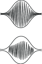
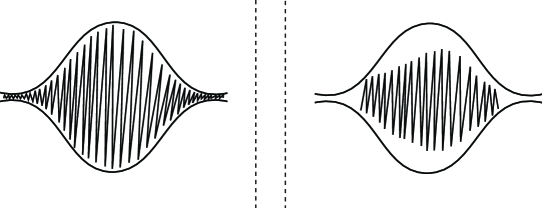
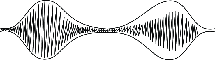
Figure 4. Given two breathers, placing them far apart, we obtain an approximate solution. Using the a-posteriori Theorem 3.6, we obtain that there is a true solution close to it. See Lemma 9.8

9.3.1. Some elementary calculations with the decay functions in Proposition 2.3

Theorem 3.11 is formulated with the special scale of decay functions $\Gamma_{\beta}$ defined by

$$\Gamma_{\beta}(i)=\begin{cases}a\ |i|^{-\alpha}\ e^{-\beta|i|}&\qquad{\rm if}\qquad i\not=0,\\ a&\qquad{\rm if}\qquad i=0\,,\end{cases}$$

with $\alpha=\alpha_{0}>N$ fixed and $0<\beta\leq\beta_{0}$.

In the proof of Proposition 2.3 in [JdlL00] it is shown that the value of $a$ can be chosen as any value less than some $a_{0}$ independent of $\beta$. Actually we have

$$a_{0}(\alpha)<\big{(}2^{\alpha+1}K_{N,\alpha}+2\big{)}^{-1},\qquad{\rm with}\quad K_{N,\alpha}=\sum_{j\in{\mathbb{Z}}^{N}\backslash\{0\}}|j|^{-\alpha}.$$

Throughout this section, we set $\Gamma=\Gamma_{2\beta_{0}}$ In the definition of both $\Gamma$ and $\Gamma_{\beta}$ we take the value of $a=\min\big{(}a_{0}(\alpha),a_{0}(2\alpha)\big{)}.$

With this choice we have the following properties:

1. if $\tilde{\beta}<\beta$ then $\Gamma_{\beta}(i)\leq\Gamma_{\tilde{\beta}}(i)$ for all $i\in{\mathbb{Z}}^{N}$.

2. if $\tilde{\beta}<\beta$ then $\displaystyle{\lim_{|m|\to\infty}}\frac{\Gamma_{\beta}(m)}{\Gamma_{\tilde{\beta}}(m)}=0.$

3. for any $\beta,\tilde{\beta}\leq\beta_{0}$

(117) $$\Gamma(i)\leq\frac{1}{a}\ \Gamma_{\beta}(i)\ \Gamma_{\tilde{\beta}}(i),\qquad i\in{\mathbb{Z}}^{N}.$$

We will encounter the quantity $\displaystyle{\sum^{r}_{k=1}}\Gamma_{\beta}(i-c_{k})$. To be able to estimate it in a convenient way, independently on $r$, we will work with sequences of sites $\underline{c}=(c_{1},c_{2},\dots)\in({\mathbb{Z}}^{N})^{\mathbb{N}}$ satisfying the property

Definition 9.5.

We say that a sequence of sites $\underline{c}$ is spatially non-resonant when for all $i\in{\mathbb{Z}}^{N}$ there exist at most two different sites $c_{p},c_{q}$ in the sequence such that $|c_{p}-i|=|c_{q}-i|$.

Remark 9.6.

If we arrange the sites $c_{k}$ in a coordinate plane of ${\mathbb{Z}}^{N}$, for instance ${\mathbb{Z}}^{2}\times\{0\}^{N-2}$, and for all $k$ we have $|(c_{k+1}-c_{k})_{2}|<|(c_{k+1}-c_{k})_{1}|$, then $\underline{c}$ is spatially non resonant according to Definition 9.5.

Lemma 9.7.

Let $\underline{c}$ be a spatially non-resonant sequence.

Let $\beta\in(0,\beta_{0})$. Then for every $i\in{\mathbb{Z}}^{N}$ and $r\geq 2$ we have

(118) $$\sum^{r}_{k=1}\Gamma_{\beta}(i-c_{k})<\frac{2}{1-e^{-\beta}}\ \max_{k}\ \Gamma_{\beta}(i-c_{k}).$$

Proof.

Let $i\in{\mathbb{Z}}^{N}$ be fixed. Let $k_{0}$ be such that $|i-c_{k_{0}}|=\min_{k}|i-c_{k}|$. By the spatially non resonant property in the sum (118) for any value $\Gamma_{\beta}(i-c_{k})$ there are at most two terms taking the same value. Then we can group the terms in pairs. Moreover if $|i-c_{p}|>|i-c_{q}|$ then

$$\Gamma_{\beta}(i-c_{p})<\Gamma_{\beta}(i-c_{q})\ e^{-\beta(|i-c_{p}|-|i-c_{q}|)}.$$

Therefore

$$\sum^{r}_{k=1}\Gamma_{\beta}(i-c_{k})<2\Gamma_{\beta}(i-c_{k_{0}})+2\sum^{\infty}_{m=1}\Gamma_{\beta}(i-c_{k_{0}})e^{-\beta m}$$

and (118) follows. ∎

9.3.2. Statement and proof of the Coupling Lemma

Lemma 9.8.

(Coupling lemma) Let $K_{\underline{\omega}_{1}}\in\mathcal{A}_{\rho,\underline{c}_{1},\Gamma_{\beta}}\cap ND_{\rm loc}(\rho,\Gamma_{\beta})$, $K_{\omega_{2}}\in\mathcal{A}_{\rho,{c}_{2},\Gamma}\cap ND_{\rm loc}(\rho,\Gamma)$, $\beta<\beta_{0}$, be the parameterizations of two invariant tori for $F$, localized around $\underline{c}_{1}$ and ${c}_{2}$ respectively, vibrating with frequencies $\underline{\omega}_{1}\in{\mathbb{R}}^{rl}$ and $\omega_{2}\in{\mathbb{R}}^{l}$ respectively.

Then, if $|m|$ is large enough, $K_{\omega_{12}}:{\mathbb{T}}^{(r+1)l}\to\mathcal{M}$ defined by

$$K_{\omega_{12}}=K_{\underline{\omega}_{1}}+\tau^{m}K_{\omega_{2}}$$

is an approximate solution of

$$F\circ K=K\circ T_{\omega_{12}}$$

in the following sense: given $0<\tilde{\beta}<\beta$ we have the estimate

$$\|F\circ K_{\omega_{12}} -K_{\omega_{12}}\circ T_{\omega_{12}}\|_{\rho,\underline{c}_{12},\Gamma_{\tilde{\beta}}}$$

(119) $$\leq\max\big{(}\|K_{\omega_{1}}\|_{\rho,\underline{c}_{1},\Gamma_{\beta}},\,\|K_{\omega_{2}}\|_{\rho,c_{2},\Gamma}\big{)},\Phi(m)$$

where $\underline{c}_{12}=(\underline{c}_{1},c_{2}-m)$, and $\Phi$ depends on $F,\underline{c}_{1},c_{2},\beta,\tilde{\beta}$ and

$$\lim_{|m|\to\infty}\Phi(m)=0.$$

Remark 9.9.

Note that the approximate torus $K_{\omega_{12}}$ is in an space of slightly slower decay than the space of the invariant tori $K_{\underline{\omega}_{1}}$ and $K_{\omega_{2}}$ since the decay estimate (119) involves the weight $\Gamma_{\tilde{\beta}}$ instead of the weight $\Gamma_{\beta}$.

It is important to emphasize that if we choose two solutions, fix a decay function slower than that of the two solutions, any target smallness for the error of the coupled solution can be accomplished by setting the translated solution far enough. In other words, we can choose all the parameters of the Lemma 9.8 and adjust all the requirements by setting the solutions far apart.

Remark 9.10.

Notice also that in Lemma 9.8, the approximate torus $K_{\omega_{12}}$ is defined on ${\mathbb{T}}^{rl}\times{\mathbb{T}}^{l}={\mathbb{T}}^{(r+1)l}$. To make the notations coherent we embed the tori ${\mathbb{T}}^{rl}$ and ${\mathbb{T}}^{l}$ into ${\mathbb{T}}^{(r+1)l}$ identifying ${\mathbb{T}}^{rl}$ with ${\mathbb{T}}^{rl}\times\{0\}$ and ${\mathbb{T}}^{l}$ with $\{0\}\times{\mathbb{T}}^{l}$ respectively. Hence if $\theta=(\theta_{1},\theta_{2})\in{\mathbb{T}}^{(r+1)l},K_{\underline{\omega}_{1}}(\theta)=K_{\underline{\omega}_{1}}(\theta_{1})$ and $K_{\omega_{2}}(\theta)=K_{\omega_{2}}(\theta_{2}).$

Remark 9.11.

For simplicity, we have stated Lemma 9.8 as joining together a breather around one site to an already constructed solution. It is possible (and perhaps more natural) to prove a lemma that asserts that given two solutions (each containing oscillations around many sites) one can displace them and obtain a very approximate solution (in a slower decay space). We leave the precise formulation and the proof to the reader.

Before proving Lemma 9.8 we establish a lemma with two technical estimates. Given $\underline{c}_{1}=(c_{1,1},\dots,c_{1,r})\in({\mathbb{Z}}^{N})^{r}$ and $c_{2},m\in{\mathbb{Z}}^{N}$ we introduce the sets of indices

$$\mathcal{I}_{1} =\big{\{}i\in{\mathbb{Z}}^{N}\,|\,\min_{k}|i-c_{1,k}|<|i+m-c_{2}|\big{\}}\,,$$

$$\mathcal{I}_{2} ={\mathbb{Z}}^{N}\setminus\mathcal{I}_{1}\,,$$

and the functions

$$B_{1}(\beta,\tilde{\beta},m) =\ \sup_{i\in\mathcal{I}_{1}}\ \frac{\Gamma_{\beta}(i+m-c_{2})}{\max_{k}\Gamma_{\tilde{\beta}}(i-c_{1,k})}\,,$$

$$B_{2}(\beta,\tilde{\beta},m) =\ \sup_{i\in\mathcal{I}_{2}}\ \frac{\max_{k}\Gamma_{\beta}(i-c_{1,k})}{\Gamma_{\tilde{\beta}}(i+m-c_{2})}\,.$$

Lemma 9.12.

If $0<\tilde{\beta}<\beta$ we have

$$\lim_{|m|\to\infty}B_{1}(\beta,\tilde{\beta},m)=\lim_{|m|\to\infty}B_{2}(\beta,\tilde{\beta},m)=0\,.$$

Proof.

First we note that if $i\in\mathcal{I}_{1}$ then

(120) $$|i+m-c_{2}|>\frac{1}{2}\min_{k}|c_{1,k}+m-c_{2}|\,.$$

Indeed, let $k_{0}$ be such that $|i-c_{1,k_{0}}|=\min_{k}|i-c_{1,k}|$. Then

$$|i+m-c_{2}| \geq|c_{1,k_{0}}+m-c_{2}|-|i-c_{1,k_{0}}|$$

$$>|c_{1,k_{0}}+m-c_{2}|-|i+m-c_{2}|$$

and hence

$$|i+m-c_{2}|>\frac{1}{2}\ |c_{1,k_{0}}+m-c_{2}|\geq\frac{1}{2}\ \min_{k}|c_{1,k}+m-c_{2}|\,.$$

Moreover, if $i\in\mathcal{I}_{1}$, by the monotonicity of $\Gamma_{\tilde{\beta}}$ we have $\max_{k}\Gamma_{\tilde{\beta}}(i-c_{1,k})>\Gamma_{\tilde{\beta}}(i+m-c_{2})$. Now

$$\frac{\Gamma_{\beta}(i+m-c_{2})}{\max_{k}\Gamma_{\tilde{\beta}}(i-c_{1,k})}<\frac{\Gamma_{\beta}(i+m-c_{2})}{\Gamma_{\tilde{\beta}}(i+m-c_{2})}\,.$$

The bound (120) shows that when $|m|\to\infty,\ |i+m-c_{2}|$ goes to infinity uniformly in $i\in\mathcal{I}_{1}$. Hence by the second property of the scale $\Gamma_{\beta}$ we obtain the first limit. The second limit is proved in an analogous way, checking first that if $i\in\mathcal{I}_{2}$

$$\min_{k}|i-c_{1,k}|\geq\frac{1}{2}\min_{k}|c_{1,k}+m-c_{2}|$$

and using that if $i\in\mathcal{I}_{2}$

$$\frac{\max_{k}\Gamma_{\beta}(i-c_{1,k})}{\Gamma_{\tilde{\beta}}(i+m-c_{2})}\leq\frac{\max_{k}\Gamma_{\beta}(i-c_{1,k})}{\max_{k}\Gamma_{\tilde{\beta}}(i-c_{1,k})}\,.$$

∎

Proof of the coupling lemma Lemma 9.8.

We denote $E(K)=F\circ K-K\circ T_{\omega_{12}}$ the error of the invariance equation for the coupled breather.

We are going to estimate the $i$-th component of $E=E(K_{\omega_{12}})$. Note that the torus $\tau^{m}K_{\omega_{2}}$ is localized around the site $c_{2}-m.$ We distinguish two cases: either $i\in\mathcal{I}_{1}$ or $i\in\mathcal{I}_{2}$. In the first case we write

$$E_{i}=F_{i}(K_{\underline{\omega}_{1}}) +\ \int^{1}_{0}\Big{[}DF\big{(}K_{\underline{\omega}_{1}}+s\tau^{m}K_{\omega_{2}}\big{)}\ \tau^{m}K_{\omega_{2}}\Big{]}_{i}\ ds$$

$$\quad-\ \big{[}K_{\underline{\omega}_{1}}\circ T_{\omega_{12}}\big{]}_{i}-\big{[}\tau^{m}K_{\omega_{2}}\circ T_{\omega_{12}}\big{]}_{i}\,.$$

We recall that $\theta=(\theta_{1},\theta_{2})\in{\mathbb{T}}^{rl}\times{\mathbb{T}}^{l}$. Since $K_{\underline{\omega}_{1}}$ does not depend on $\theta_{2}$ then $F(K_{\underline{\omega}_{1}})=K_{\underline{\omega}_{1}}\circ T_{\omega_{12}}$. Therefore

$$\|E_{i}\|_{\rho} \leq\sum_{j}\|F\|_{C^{1}_{\Gamma}}\,\Gamma(i-j)\,\|K_{\omega_{2}}\|_{\rho,c_{2},\Gamma}\ \Gamma(j+m-c_{2})$$

$$\quad+\|K_{\omega_{2}}\|_{\rho,c_{2},\Gamma}\ \Gamma(i+m-c_{2})$$

$$\leq\big{(}\|F\|_{C^{1}_{\Gamma}}+1\big{)}\,\|K_{\omega_{2}}\|_{\rho,c_{2},\Gamma}\ \Gamma(i+m-c_{2})\,.$$

Similarly, if $i\in\mathcal{I}_{2}$ we expand $F$ around $\tau^{m}\,K_{\omega_{2}}$ and we obtain

$$\|E_{i}\|_{\rho}\leq\Big{(}\frac{2}{1-e^{-\beta}}\,\|F\|_{C^{1}_{\Gamma}}+1\Big{)}\,\|K_{\underline{\omega}_{1}}\|_{\rho,\underline{c}_{1},\Gamma_{\beta}}\,\max_{k}\,\Gamma_{\beta}(i-c_{1,k})\,.$$

We take $\tilde{\beta}<\beta$ and we compute

$$\|E\|_{\rho,\underline{c}_{12},\Gamma_{\tilde{\beta}}} =\ \max\Big{(}\sup_{i\in\mathcal{I}_{1}}\ \min\big{(}\min_{k}\,\Gamma^{-1}_{\tilde{\beta}}(i-c_{1,k})\,,\,\Gamma^{-1}_{\tilde{\beta}}(i+m-c_{2})\big{)}\,\|E_{i}\|_{\rho}\,,$$

$$\qquad\sup_{i\in\mathcal{I}_{2}}\ \min\big{(}\min_{k}\ \Gamma^{-1}_{\tilde{\beta}}(i-c_{1,k}),\,\Gamma^{-1}_{\tilde{\beta}}(i+m-c_{2})\big{)}\,\|E_{i}\|_{\rho}\Big{)}$$

$$\leq\ C\ \max\Big{(}\sup_{i\in\mathcal{I}_{1}}\ \min_{k}\ \Gamma^{-1}_{\tilde{\beta}}(i-c_{1,k})\,\Gamma(i+m-c_{2}),$$

$$\qquad\sup_{i\in\mathcal{I}_{2}}\,\Gamma^{-1}_{\tilde{\beta}}(i+m-c_{2})\ \max_{k}\ \Gamma_{\beta}(i-c_{1,k})\Big{)}$$

$$=C\ \max\big{(}B_{1}(2\beta_{0},\tilde{\beta},m),\ B_{2}(\beta,\tilde{\beta},m)\big{)}\,,$$

where

$$C=\Big{(}\frac{2}{1-e^{-\beta}}\ \|F\|_{C^{1}_{\Gamma}}+1\Big{)}\ \max\Big{(}\|K_{\underline{\omega}_{1}}\|_{\rho,\underline{c}_{1},\Gamma_{\beta}}\,,\ \|K_{\omega_{2}}\|_{\rho,c_{2},\Gamma}\Big{)}\,.$$

∎

9.3.3. Statement and proof of Lemma 9.13. Verifying the non-degeneracy condition of the coupled solutions

In this section, we verify the nondegeneracy conditions provided that $\varepsilon$ is small enough and that $K$ is sufficiently close to an uncoupled solution with all the sites far enough apart. That is, we consider situations when we are close to the completely uncoupled solution.

The result Lemma 9.13 will be clear because all the uncoupled solutions for the uncoupled dynamics satisfy the non-degeneracy assumptions. The change of the non-degeneracy assumptions between this uncoupled case can be controlled by elementary perturbation theories. Thanks to the systematic use of our framework, we have perturbation theories which are uniform on the excited sites.

Let $\underline{c},\underline{\omega}$ be sequences of $r$ sites and frequencies. We consider $k_{\omega_{i}}$, parameterizations of invariant tori w.r.t. $f_{0}$, the time-one map of just one site. We denote

$$K^{*}=\sum_{i=1}^{r}\tau^{c_{i}}k_{\omega_{i}}$$

We note that $F_{0}\circ K^{*}=K^{*}\circ T_{\underline{\omega}}$ and that $K^{*}$ is uniformly non degenerate.

The hyperbolic splitting for $F_{0}\circ K^{*}$ is

(121) $$\Pi^{s,c,u}=\oplus_{i\in{\mathbb{Z}}^{N}}\Pi^{s,c,u}_{i}$$

where $\Pi^{s,c,u}_{i}$ is the splitting corresponding to the $i$ torus. If $i$ is an index in $\underline{c}$, then we have $\Pi^{c}_{i}={\rm Id}_{{\mathbb{R}}^{2l}}$, $\Pi^{s}_{i}=0$, $\Pi^{u}_{i}=0$. Otherwise, one gets $\Pi^{c}_{i}=0$, and $\Pi^{s}_{i},\Pi^{s}_{i}$ are the projections corresponding to the stable and unstable directions at the fixed point.

Notice also that the $rl\times rl$ matrix $DK^{\top}DK$ is block diagonal. The diagonal has $r$ $l\times l$ blocks $\{Dk_{\omega_{i}}^{\top}Dk_{\omega_{i}}\}_{i=1}^{r}$.

Lemma 9.13.

(Hyperbolicity conditions) Assume the hypothesis and the notation in Theorem 3.11. In particular, $F_{\varepsilon}$ is an analytic family of exact symplectic maps in $C^{2}_{\Gamma}({\mathcal{B}})$. Let $K\in{\mathcal{A}}_{\rho,\underline{c},\tilde{\Gamma}}$ with $\tilde{\Gamma}<\Gamma_{\beta}$ for $\beta<\beta_{0}$.

Assume that $\varepsilon$, $\eta\equiv\|K-K^{*}\|_{\rho,\underline{c},\tilde{\Gamma}}$ are smaller than a number that is independent of $\underline{c}$ and of $\Gamma$ – it depends only on $\|F\|_{C^{2}_{\Gamma}({\mathcal{B}}_{1})}$, $\|\partial_{\varepsilon}F\|_{C^{2}_{\Gamma}({\mathcal{B}}_{1}\times\{|\varepsilon|\leq\varepsilon^{*}\})}$, $\|\partial_{\varepsilon}^{2}F\|_{C^{2}_{\Gamma}({\mathcal{B}}_{1}\times\{|\varepsilon|\leq\varepsilon^{*}\})}$ and the hyperbolicity constants of the uncoupled splitting.

Then, $K$ and $F_{\varepsilon}$ satisfy the non-degeneracy conditions in Definition 3.1 with uniform constants.

Proof.

We make the elementary remark

(122) $$DF_{\varepsilon}\circ K=DF_{0}\circ K^{*}+\big{(}DF_{0}\circ K-DF_{0}\circ K^{*}\big{)}+\big{(}DF_{\varepsilon}\circ K-DF_{0}\circ K\big{)}$$

and we will control the terms in parenthesis.

By the estimates in composition in Section A.5, we obtain that:

$$\begin{split}\|DF_{0}\circ K-DF_{0}\circ K^{*}\|_{\rho,\underline{c},\tilde{\Gamma}}&\leq C\|K-K^{*}\|_{\rho,\underline{c},\tilde{\Gamma}}\\ \|DF_{\varepsilon}\circ K-DF_{0}\circ K\|_{\rho,\underline{c},\tilde{\Gamma}}&\leq C|\varepsilon|\end{split}$$

so we obtain that $\|DF_{\varepsilon}\circ K-DF_{0}\circ K^{*}\|_{\rho,\underline{c},\tilde{\Gamma}}$ is small.

The splitting indicated in (121) is invariant for $DF_{0}$. Hence, it is approximately invariant for $DF_{\varepsilon}\circ K$ and this satisfies the conditions for approximately invariant splittings Definition 3.2.

We note that Proposition 4.2 ensures that, if $\varepsilon$ and $\eta$ are small enough, there is an invariant splitting satisfying Definition 3.1. ∎

9.3.4. Statement and proof of Lemma 9.14. Verifying the non-degeneracy assumptions of coupled solutions

Lemma 9.14.

(Twist conditions) Assume that $K_{1},K_{2}$ are embeddings in ${\mathcal{A}}_{\rho,\underline{c}_{1},\Gamma_{\beta}}$, ${\mathcal{A}}_{\rho,\underline{c}_{2},\Gamma_{\beta}}$, resp. both $\underline{c}_{1}$, $\underline{c}_{2}$ being finite sequences, and $\Gamma_{\beta}$ as before. Assume that $K_{1}$, $K_{2}$ satisfy the non-degeneracy conditions in Definition 3.4.

Then, for $m$ sufficiently large,

$$\tilde{K}(\theta_{1},\theta_{2})=K_{1}(\theta_{1})+\tau^{m}K_{2}(\theta_{2})$$

satisfies the non-degeneracy assumptions in Definition 3.4. Furthermore, the non-degeneracy constants of $\tilde{K}$ can be made as close to desired to the constants verified both by $K_{1},K_{2}$ if we choose $|m|$ large enough.

We will be using the notation that $n_{1}$ is the number of sites in $\underline{c}_{1}$ and that $\theta_{1}$ stands for all the $n_{1}\times l$ variables corresponding to all the sites in $\underline{c}_{1}$. Similarly for $K_{2}$.

Proof.

We introduce the notation that $\Phi(m)$ stands for any quantity (vector, matrix, function, etc. ) which can be made arbitrarily small by making $m$ large.

We start by estimating the non-degeneracy condition of the embedding.

We see that the $l(n_{1}+n_{2})\times l(n_{1}+n_{2})$ matrix $D\tilde{K}^{\top}D\tilde{K}$ splits naturally into blocks depending on whether we take derivatives with respect to variables in $\theta_{1}$ or in $\theta_{2}$:

(123) $$D\tilde{K}^{\top}D\tilde{K}=\begin{pmatrix}D_{\theta_{1}}K_{1}^{\top}D_{\theta_{1}}K_{1}&D_{\theta_{1}}K^{\top}_{1}\tau^{m}D_{\theta_{2}}K_{2}\\ \tau^{m}D_{\theta_{2}}K_{2}^{\top}D_{\theta_{1}}K_{1}&D_{\theta_{2}}\tau^{m}K^{\top}_{2}D_{\theta_{2}}\tau^{m}K_{2}\end{pmatrix}\,.$$

Since

$$D_{\theta_{2}}\tau^{m}K^{\top}_{2}D_{\theta_{2}}\tau^{m}K_{2}=D_{\theta_{2}}K^{\top}_{2}D_{\theta_{2}}K_{2}$$

we see that the diagonal elements of $D\tilde{K}^{\top}D\tilde{K}$ are precisely those of the uncoupled system and are therefore invertible.

We will show that the non-diagonal elements in (123) can be made arbitrarily small by choosing $m$ large enough. Then, it will follow that $D\tilde{K}^{\top}D\tilde{K}$ is invertible and that

(124) $$\tilde{N}=(D\tilde{K}^{\top}D\tilde{K})^{-1}=\begin{pmatrix}(D_{\theta_{1}}K_{1}^{\top}D_{\theta_{1}}K_{1})^{-1}&0\\ 0&(D_{\theta_{2}}K^{\top}_{2}D_{\theta_{2}}K_{2})^{-1}\end{pmatrix}+\Phi(m)=$$

$$\begin{pmatrix}N_{1}&0\\ 0&N_{2}\end{pmatrix}+\Phi(m).$$

We estimate the off-diagonal elements of (123). We observe that, we can estimate the entries of $n_{1}l\times n_{2}l$ upper right block as follows:

$$\Big{|}\big{(}D_{\theta_{1}} K^{\top}_{1}\,\tau^{m}\,D_{\theta_{2}}K_{2}\big{)}_{p,q}\Big{|}\leq\sum_{i}\Big{|}\frac{\partial K_{1,i}}{\partial\theta_{1,p}}\ \frac{\partial K_{2,i+m}}{\partial\,\theta_{2,q}}\Big{|}$$

$$\leq\ \|DK_{1}\|_{\rho,\underline{c}_{1},\Gamma_{\beta}}\|DK_{2}\|_{\rho,\underline{c}_{2},\Gamma}\sum_{i}\,\max_{k}\ \Gamma_{\beta}(i-c_{1,k})\ \max_{l}\Gamma(i+m-c_{2,l})$$

$$\leq\frac{2}{1-e^{-\beta}}\|DK_{1}\|_{\rho,\underline{c}_{1},\Gamma_{\beta}}\ \|DK_{2}\|_{\rho,c_{2},\Gamma}\ \max_{k,l}\ \Gamma_{\beta}(c_{2,l}-m-c_{1,k})\,.$$

Since the block is finite dimensional, making the previous elements small enough makes its norm small.

Estimates for the lower left block are obtained just noticing that it is the transposed of the upper right one.

Now, we turn to estimating the twist condition. Again the strategy is very similar to the one used in checking the non-degeneracy condition. We just check that the matrix we need to invert is arbitrarily close (by taking $|m|$ large enough) to a matrix which is block diagonal and whose blocks correspond to the non-degeneracy conditions of each of the uncoupled solutions.

We proceed to estimate systematically all the ingredients of $A$ defined in (20). We have first

$$\tilde{P}(\theta) =\big{(}D_{\theta_{1}}K_{1},\ \ D_{\theta_{2}}\,[\tau^{m}\,K_{2}]\big{)}\begin{pmatrix}N_{1}&0\\ 0&N_{2}\end{pmatrix}\,+\Phi(m)$$

$$=(P_{1},P_{2})+\Phi(m)\,.$$

Since $N_{1}$ and $N_{2}$ are finite dimensional matrices, $P_{1}$ and $P_{2}$ are also in ${\mathcal{A}}_{\rho,\underline{c}_{1},\Gamma}$ and ${\mathcal{A}}_{\rho,\underline{c}_{2},\Gamma}$, respectively.

Using that $J_{\infty}$ is uncoupled and constant for the models (26) we are considering now, we can write:

(125) $$\begin{split}(DF(J^{c})^{-1})&\ \big{(}\tilde{K}(\theta)\big{)}\ P_{1}(\theta_{1})\\ &=(DF(J^{c})^{-1})\ \big{(}K_{1}(\theta_{1})\big{)}\ P_{1}(\theta_{1})\\ &\quad+\int^{1}_{0}(D^{2}F(J^{c})^{-1})\,\big{(}K_{1}(\theta_{1})+s\tau^{m}K_{2}(\theta_{2})\big{)}\big{(}\tau^{m}K_{2}(\theta_{2}),P_{1}(\theta_{1})\big{)}\,ds\end{split}$$

(126) $$\begin{split}(DF(J^{c})^{-1})\ \big{(}\tilde{K}&(\theta)\big{)}\ P_{2}(\theta_{2})\\ &=(DF(J^{c})^{-1})\ \big{(}\tau^{m}K_{2}(\theta_{2})\big{)}\ P_{2}(\theta_{2})\\ &\quad+\int^{1}_{0}(D^{2}F(J^{c}))\,\big{(}sK_{1}(\theta_{1})+\tau^{m}K_{2}(\theta_{2})\big{)}\ \big{(}K_{1}(\theta_{1}),\,P_{2}(\theta_{2})\big{)}\,ds\,.\end{split}$$

We denote $T_{21}$ and $T_{12}$ the integral terms in (125) and (126) respectively. We bound from above the $i$-th component of $T_{21}$ by

$$\|(J^{c})^{-1}\|\ \sum_{j,n}\ \left|\frac{\partial^{2}F_{i}}{\partial x_{j}\ \partial x_{n}}\right|_{\rho}\ \left|(K_{2})_{j+m}\right|_{\rho}\left|(P_{1})_{n}\right|_{\rho}$$

$$\leq\|(J^{c})^{-1}\|\ \|F\|_{C^{2}_{\Gamma}}\ \|K_{2}\|_{\rho}\ \|P_{1}\|_{\rho,\underline{c}_{1},\Gamma_{\beta}}$$

$$\quad\times\sum_{j,n}\ \min\big{(}\Gamma(i-j),\Gamma(i-n)\big{)}\ \max_{k,l}\Gamma(j+m-\underline{c}_{2,l})\ \Gamma_{\beta}(n-c_{1,k})\,.$$

The last sum is bounded by

$$\frac{4}{1-e^{-\beta}}\ \max_{k,l}\Gamma_{\beta}(i+m-c_{2,l})\cdot\Gamma_{\beta}(i-c_{1,k})\leq\Phi(m).$$

Indeed, let ${\mathcal{J}}_{1}(i)=\{j,n\in{\mathbb{Z}}^{N}\mid|i-j|\leq|i-n|\}$ and ${\mathcal{J}}_{2}(i)={\mathbb{Z}}^{N}\setminus{\mathcal{J}}_{1}(i)$. Using that $\Gamma(i)\leq\frac{1}{a}\Gamma_{\beta}(i)\Gamma_{\beta}(i)$ the previous sum is bounded by

$$\sum_{j,n\in{\mathcal{J}}_{1}(i)}\Gamma(i-j)\max_{l}\Gamma(j+m-c_{2,l})\ \max_{k}\ \Gamma_{\beta}(n-c_{1,k})$$

$$\quad+\sum_{j,n\in{\mathcal{J}}_{2}(i)}\Gamma(i-n)\max_{l}\Gamma(j+m-c_{2,l})\ \max_{k}\ \Gamma_{\beta}(n-c_{1,k})$$

$$\leq\frac{2}{a}\sum_{j\in{\mathbb{Z}}^{N}}\Gamma_{\beta}(i-j)\max_{l}\Gamma(j+m-c_{2,l})\ \sum_{n\in{\mathbb{Z}}^{N}}\Gamma_{\beta}(i-n)\max_{k}\ \Gamma_{\beta}(n-c_{1,k}).$$

Analogously $T_{12}$ is bounded by

$$\|(J^{c})^{-1}\|\ \|F\|_{C^{2}_{\Gamma}}\ \|K_{1}\|_{\rho,\underline{c}_{1},\Gamma_{\beta}}\ \|P_{2}\|_{\rho}\ \frac{4}{1-e^{-\beta}}\ \max_{k,l}\ \Gamma_{\beta}(i+m-c_{2,l})\ \Gamma_{\beta}(i-c_{1,k}).$$

Note that $P^{\top}_{1}(\theta+\omega)\ T_{21}(\theta)$ and $P^{\top}_{2}(\theta+\omega)\ T_{12}(\theta)$ are bounded by $C\ \displaystyle\max_{k,l}\ \Gamma_{\beta}(c_{1,k}+m-c_{2,l})$, where $C$ depends on $\|(J^{c})^{-1}\|,\ \|F\|_{C^{2}_{\Gamma}},\ \|K_{1}\|_{\rho,\underline{c}_{1},\Gamma_{\beta}},$ $\|K_{2}\|_{\rho,\underline{c}_{2},\Gamma},\ \|P_{1}\|_{\rho,\underline{c}_{1},\Gamma_{\beta}}$ and $\|P_{2}\|_{\rho,\underline{c}_{2},\Gamma}$.

Also note that

$$\big{|}\big{[}P_{1}(\theta+\omega)^{\top}\ (J^{c})^{-1}(K(\theta))P_{2}(\theta)\big{]}_{i}\big{|} \leq\|(J^{c})^{-1}\|\ \|P_{1}\|_{\rho,\underline{c}_{1},\Gamma_{\beta}}\ \|P_{2}\|_{\rho,\underline{c}_{2},\Gamma}$$

$$\quad\times\sum_{i\in{\mathbb{Z}}^{N}}\max_{k,l}\ \Gamma_{\beta}(i-c_{1,k})\ \Gamma(i+m-c_{2,l})$$

$$\leq C\ \max_{k.l}\ \Gamma_{\beta}\ (c_{2,l}-m-c_{1,k}).$$

Now we consider the terms $P^{\top}_{1}(\theta+\omega)\ (DF\tilde{(}J^{c})^{-1})\ \big{(}\tilde{K}(\theta)\big{)}\ P_{2}(\theta)$ and $P^{\top}_{2}(\theta+\omega)\ (DF\tilde{(}J^{c})^{-1})\ \big{(}\tilde{K}(\theta)\big{)}\ P_{1}(\theta)$. We evaluate the first one, the other being analogous. Given $n\in\{1,\dots,r\}$,

$$\big{|}\big{[}P^{\top}_{1}\ (\theta+\omega)\,(DFJ^{c})\,\big{(}\tilde{K}(\theta)\big{)}\ P_{2}(\theta)\big{]}_{n}\big{|}$$

$$\leq\sum_{i,j}\ \big{|}(P_{1})_{i,n}\big{|}_{\rho}\ \|(J^{c})^{-1}\|\ \Big{\|}\frac{\partial F_{i}}{\partial x_{j}}\Big{\|}_{\rho}\ |(P_{2})_{j}|_{\rho}$$

$$\leq\|F\|_{C^{1}_{\Gamma}}\ \|(J^{c})^{-1}\|\ \|P_{1}\|_{\rho,\underline{c},\Gamma_{\beta}}\ \|P_{2}\|_{\rho,c_{2},\Gamma}\,\sum_{i,j}\,\max_{k,l}\ \Gamma_{\beta}(i-c_{1,k})\ \Gamma(i-j)\ \Gamma(j+m-c_{2,l})$$

$$\leq C\ \max_{k}\ \Gamma_{\beta}\,(c_{1,k}+m-c_{2,l}).$$

With all these previous estimates we can write:

$$A =\big{[}(P_{1},P_{2})\circ T_{\omega}+\Phi(m)\big{]}^{\top}(DFJ^{c})\,(\tilde{K})\ \big{[}(P_{1},P_{2})+\Phi(m)\big{]}-J^{c}P\circ T_{\omega}$$

$$=\begin{pmatrix}\scriptstyle P^{\top}_{1}\circ T_{\underline{\omega}_{1}}\big{[}(DF(J^{c})^{-1})\,(K_{1})\ P_{1}\big{]}-(J^{c})^{-1}\,P_{1}\circ T_{\underline{\omega}_{1}}&0\\[5.69054pt] 0&\scriptstyle P^{\top}_{2}\circ T_{\omega_{2}}\big{[}(DFJ^{c})\,(K_{2})\ P_{2}\big{]}-(J^{c})^{-1}\,P_{2}\circ T_{\omega_{2}}\end{pmatrix}$$

$$+\Phi(m)=\begin{pmatrix}A_{1}&0\\ 0&A_{2}\\ \end{pmatrix}+\Phi(m)$$

which shows that it is invertible if $|m|$ is big enough and that the norm of the inverse of $A$ can be bounded from above by $\max(|A_{1}^{-1}|,|A_{2}^{-1}|)+\tilde{\Phi}_{m}$.

∎

The estimates about the non-degeneracy with respect to parameters in the construction are automatic since, in the construction in Section C, which is the one we use here, the matrix $Q$ is the identity, whose norm is bounded by $1$ independently of the number of sites considered and independently of the $K$ considered.

9.4. Adding oscillating sites inductively

Recall that we are assuming that $\varepsilon\leq\varepsilon^{*}$ and that we have a set $\Xi_{1}(\varepsilon^{*})\subset D(\nu_{0},\kappa_{0})\subset{\mathbb{R}}^{l}$ of positive measure such that, for all $\omega\in\Xi_{1}(\varepsilon^{*})$, the system (26) has a breather of frequency $\omega$ in ${\mathcal{A}}_{\rho,\{0\},\Gamma_{\beta}}$. The non-degeneracy and hyperbolicity constants of all these solutions are uniformly bounded.

The remaining part to be shown is that given a sequence $\underline{\omega}\in\mathcal{D}\cup\Xi_{1}^{*}(\varepsilon^{*})^{\infty}$, we can find a sequence of tori parameterized by $K_{\omega^{(n)}}\in{\mathcal{A}}_{\rho_{n},\underline{c}^{(n)},\Gamma_{\beta_{n}}}$ for a suitable sequence of centers $\underline{c}^{(n)}$. Here we have that

$$\omega^{(n)}=(\omega_{1},\ldots,\omega_{n})$$

is the sequence of truncations of $\underline{\omega}$ and $\rho_{n},\beta_{n}$ are strictly decreasing sequences so that $\rho_{n}\to\rho_{\infty}>0$, $\beta_{n}\to\beta_{\infty}>0$.

Our unknowns are $\rho_{n},\beta_{n}$, the infinite sequence of centers $\underline{c}^{(n)}$ and the embeddings $K_{\omega^{(n)}}$ .

The choices of $\rho_{n},\beta_{n}$ are almost irrelevant for our purposes, so we choose them right away. For example we take $0<\rho_{\infty}<\rho_{0}$, $0<\beta_{\infty}<\beta_{0}$ and $\rho_{n}=\rho_{\infty}+2^{-n}(\rho_{0}-\rho_{\infty})$, $\beta_{n}=\beta_{\infty}+2^{-n}(\beta_{0}-\beta_{\infty})$,

So that now, our only task is to choose a sequence of sites $\underline{c}^{(n)}$ (without loss of generality, we will assume $c_{1}=0$), such that, recursively, we have that taking $c_{n+1}$ far apart from the previous sites, $K_{\underline{\omega}^{(n)}}+\tau^{-c_{n+1}}K_{\omega_{n+1}}$ is a very approximate solution of the invariance equation which, furthermore, satisfies uniform hyperbolicity and non-degeneracy conditions. Then, an application of Theorem 3.6 will produce a true solution $K_{\underline{\omega}^{(n+1)}}$.

Of course, we will have to recover the inductive hypothesis we have made to construct this sequence. We will show that, we can ensure that $\|K_{\underline{\omega}^{(n)}}-K^{*}\|_{\rho_{n},\underline{c}^{(n)},\Gamma_{\beta_{n}}}\leq\eta/2$ where $\eta>0$ is the constant introduced in Lemma 9.13 and $K^{*}_{n}=K_{\omega_{1}}+\tau^{-c_{2}}K_{\omega_{2}}+\cdots\tau^{-c_{n}}K_{\omega_{n}}$.

After this sequence of tori with increasing number of frequencies is produced, we will have to study the limit of the sequence and show that it solves the invariance equation (this will be accomplished in Section 9.5). Note that, since each step changes the number of centers, the convergence of the embeddings cannot be uniform (even in a space of decay functions). Nevertheless, we will show that there is coordinatewise convergence and that this is enough to show that the limit satisfies the invariance equation.

We note that the existence of the sequence and the study of the limit will be accomplished because if we place the centers very far apart from the previously placed ones, we can obtain that the error is small enough to beat the smallness requirements of Theorem 3.6, to ensure that the non-degeneracy and hyperbolicity constants deteriorate an arbitrarily small amount and to ensure the passage to the limit, so that, by recursively assuming that the new center is far away from all the previously placed ones, we can ensure any smallness conditions we wish on the error, on the increment of the distance from the uncoupled solution and on the deterioration of the non-degeneracy and hyperbolicity constants.

We start with $K_{\omega_{1}}$ and $K_{\omega_{2}}$ localized at the node $c_{1}=0$ and $c_{2}$ respectively and we take $|c_{2}|$ big enough so that

$$\tilde{K}=K_{\omega_{1}}+\tau^{-c_{2}}\ K_{\omega_{2}}$$

is a sufficiently approximate solution of $F\circ K-K\circ T_{{\underline{\omega}}^{(2)}}=0$ and satisfies both the spectral and the twist non-degeneracy conditions. Then Theorem 3.6 provides the existence of a true invariant torus $K_{{\underline{\omega}}^{(2)}}\in{\mathcal{A}}_{\rho_{2},\underline{c}^{(2)},\Gamma_{\beta_{2}}}$ such that it is non-degenerate and

$$e=\|K_{\underline{\omega}^{(2)}}-\tilde{K}\|_{\rho_{2},\underline{c}^{(2)},\Gamma_{\beta_{2}}}$$

is small. Actually it can be made as small as we want by taking $|c_{2}|$ sufficiently big. Remembering that $(\omega_{1},\omega_{2})$ is Diophantine (and chosen from the start of the procedure), we see that Theorem 3.6 guarantees that, if we make the initial error small enough, we can produce a solution $K_{\underline{\omega}^{(2)}}$ of the invariance equation with frequency $\underline{\omega}^{(2)}$.

In the $n+1$ step of the process we assume we have the torus $K_{{\underline{\omega}}^{(n)}}\in{\mathcal{A}}_{\rho_{n},\underline{c}^{(n)},\Gamma_{\beta_{n}}}$ localized around the nodes $\underline{c}^{(n)}=(c_{1},\dots,c_{n})$, which is non-resonant, that is $K{{}_{\underline{\omega}^{(n)}}}\in ND_{\rm loc}(\rho_{n},\Gamma_{\beta_{n}})$

We consider the parameterization

$$\tilde{K}(\theta)-K{{}_{\underline{\omega}^{(n)}}}(\theta_{1})+\tau^{m_{n+1}}\ K_{\omega_{n+1}}(\theta_{2}),\qquad\theta=(\theta_{1},\theta_{2})\in{\mathbb{T}}^{nl}\times{\mathbb{T}}^{l},$$

as an approximation for the new torus, which we will denote $K{{}_{\underline{\omega}^{(n+1)}}}$, with some $m_{n+1}\in{\mathbb{Z}}^{N}$.

By the coupling lemma (Lemma 9.8) if we take a suitable $m_{n+1}$ big enough we obtain

$$E_{n+1}=F\circ\tilde{K}-\tilde{K}\circ T_{\underline{\omega}^{(n+1)}}$$

as small as we want. In particular we take $0<\delta_{n+1}<\min\,\big{(}1,\rho_{n}/12,\ (\rho_{n+1}-\rho_{n})/6\big{)}$ and we require

$$C\kappa^{4}_{n+1}\ \delta^{-4\nu_{n+1}}_{n+1}\ \|E_{n+1}\|_{\rho_{n+1},\underline{c}^{(n+1)},\Gamma_{\beta_{n+1}}}\leq 1\,,$$

and

$$C\kappa^{2}_{n+1}\ \delta^{-2\nu_{n+1}}_{n+1}\ \|E_{n+1}\|_{\rho_{n+1},\underline{c}^{(n+1)},\Gamma_{\beta_{n+1}}}\leq\frac{e}{2^{n-1}}\,.$$

We denote $c_{n+1}=-m_{n+1}$. Then Theorem 3.6 provides a true invariant torus $K_{\underline{\omega}^{(n+1)}}\in{\mathcal{A}}_{\rho_{n+1},\underline{c}^{(n+1)},\Gamma_{\beta_{n+1}}}$, non-degenerate and satisfying the estimate

(127) $$\|K_{\underline{\omega}^{(n+1)}}-\tilde{K}\|_{\rho_{n+1},\underline{c}^{(n+1)},\Gamma_{\beta_{n+1}}}\leq\frac{e}{2^{n-1}}\,.$$

9.5. Passage to the limit (Part B of Theorem 3.11)

The issue now is to study the limit $n\rightarrow\infty$. Thanks to our weighted spaces and the fact that the solutions we construct have bumps whose distance from each other tends to infinity fast enough, we can prove the following Lemma 9.15 which establishes that for any bounded sets in the lattice, the trajectories of the particles in this set converge uniformly.

Lemma 9.15.

The sequence $\big{\{}K_{\underline{\omega}^{(n)}}\big{\}}_{n\geq 1}$ converges component-wise and uniformly on every compact set of $({\mathbb{T}}^{l})^{\mathbb{N}}$. We denote $K_{\underline{\omega}}$ the limit obtained in this sense. Furthermore, each component of $K_{\underline{\omega}}$ is analytic from $({\mathbb{T}}^{l})^{\mathbb{N}}$ into $M$.

Remark 9.16.

Here, by analytic on the infinite dimensional torus $({\mathbb{T}}^{l})^{\mathbb{N}}$, we mean $K_{\underline{\omega}}$ writes component-wise

$$(K_{\underline{\omega}})_{i}(\underline{\theta})=\sum_{n\geq 0}(H^{(n)})_{i}(\theta_{1},\dots,\theta_{n}),$$

where $(H^{(n)})_{i}(\theta_{1},\dots,\theta_{n})$ are analytic in the usual sense on $({\mathbb{T}}^{l})^{n}$ and moreover we have

$$\sum_{n\geq 0}\|(H^{(n)})_{i}\|_{\rho_{n}}<\infty,$$

where $D_{\rho_{n}}\supset({\mathbb{T}}^{l})^{n}$.

Proof.

We represent $K_{\underline{\omega}}(\underline{\theta})$ as

$$\lim_{n\to\infty}\ K_{\underline{\omega}^{(n)}}(\underline{\theta})$$

(128) $$=K_{\omega_{1}}(\theta_{1})+\sum^{\infty}_{n=1}\ \big{[}K_{\underline{\omega}^{(n+1)}}\ (\theta_{1},\dots,\theta_{n+1})-K_{\underline{\omega}^{(n)}}(\theta_{1},\dots,\theta_{n})\big{]}\,.$$

We fix $i\in{\mathbb{Z}}^{N}$ and we estimate the $i$-th component of $K_{\underline{\omega}^{(n+1)}}-K_{\underline{\omega}^{(n)}}$. By the triangle inequality

$$\big{|}\big{[}K_{\underline{\omega}^{(n+1)}}-K_{\underline{\omega}^{(n)}}\big{]}_{i}\big{|}_{\rho_{n+1}} \leq\big{|}\big{[}K_{\underline{\omega}^{(n+1)}}-K_{\underline{\omega}^{(n)}}-\tau^{m_{n+1}}\ K_{\omega_{n+1}}\big{]}_{i}\big{|}_{\rho_{n+1}}$$

(129) $$\quad+\big{|}\tau^{m_{n+1}}\ K_{\omega_{n+1}}\big{]}_{i}\big{|}_{\rho_{n+1}}\,.$$

The first term in the right-hand side of (129) is bounded by

$$\frac{e}{2^{n-1}}\ \max_{1\leq k\leq n+1}\ \Gamma_{\beta_{n+1}}\ (i-c_{k})$$

and the second one is bounded by (see (127))

$$\big{|}\big{[}\tau^{m_{n+1}}\ K_{\omega_{n+1}}]_{i}\big{|}_{\rho_{1}}=\big{|}\big{[}K_{\omega_{n+1}}]_{i+m_{n+1}}|_{\rho_{1}}\leq\|K_{\omega_{n+1}}\|_{\rho_{1},0,\Gamma}\ \Gamma(i+m_{n+1}).$$

This implies that the $i$-th component of the sum in (128) is bounded by

(130) $$\sum^{\infty}_{n=1}\ \frac{e}{2^{n-1}}+\sum^{\infty}_{n=1}\ \|K_{\omega_{n+1}}\|_{\rho_{1},0,\Gamma}\ \Gamma(i+m_{n+1})\,.$$

Therefore the $i$-th component of (128) converges uniformly on compact sets of $({\mathbb{T}}^{l})^{\mathbb{N}}$ and $K_{\underline{\omega}}$ is analytic in the sense of Remark 9.16. ∎

The following result proves that $K_{\underline{\omega}}$ is a solution of the invariance equation and therefore is an almost-periodic function of the initial system.

Lemma 9.17.

The limit function $K_{\underline{\omega}}$ satisfies

$$F\circ K_{\underline{\omega}}=K_{\underline{\omega}}\circ T_{\underline{\omega}}$$

component-wise.

Proof.

For every $n\in{\mathbb{N}}$ one has

(131) $$F\circ K_{\underline{\omega}^{(n)}}=K_{\underline{\omega}^{(n)}}\circ T_{\underline{\omega}^{(n)}}\,.$$

We fix a component $i\in{\mathbb{Z}}^{N}$. The passage to the limit in the right-hand side of (131) is immediate. For the left-hand side we take $n_{0}$ such that $|c_{n}|>|i|$ for $n>n_{0}$. Then for $n>n_{0}$ we have

(132) $$\big{|}F_{i}\circ K_{\underline{\omega}^{(n)}}-F_{i}\circ K_{\underline{\omega}}\big{|}_{\rho_{\infty}}\leq\sum_{j}\ \Big{|}\frac{\partial F_{i}}{\partial x_{j}}\Big{|}\ \big{|}\big{[}K_{\underline{\omega}^{(n)}}-K_{\underline{\omega}}\big{]}_{j}\big{|}_{\rho_{\infty}}\,.$$

We estimate

$$\big{|}\big{[}K_{\underline{\omega}^{(n)}}-K_{\underline{\omega}}\big{]}_{j}\big{|}_{\rho_{\infty}}\leq\sum^{\infty}_{p=n}\ \big{|}\big{[}K_{\underline{\omega}^{(p)}}-K_{\underline{\omega}^{(p+1)}}\big{]}_{j}\big{|}_{\rho_{p+1}}$$

$$\leq\sum^{\infty}_{p=n}\ \Big{[}\frac{e}{2^{p-1}}\ \max_{1\leq k\leq p+1}\ \Gamma_{\beta_{p+1}}\ (j-c_{k})+\big{|}\big{[}\tau^{-c_{p+1}}\ K_{\omega_{p+1}}\big{]}_{j}\big{|}_{\rho_{p+1}}\Big{]}$$

$$\leq\sum^{\infty}_{p=n}\ \Big{[}\frac{e}{2^{p-1}}\ \max_{1\leq k\leq p+1}\ \Gamma_{\beta_{\infty}}\ (j-c_{k})+\|K_{\omega_{p+1}}\|_{\rho_{1},0,\Gamma}\Gamma(j-c_{p+1})\Big{]}\,.$$

Then (132) is bounded by

$$\sum^{\infty}_{p=n} \|F\|_{C^{1}_{\Gamma}}\Big{[}\frac{e}{2^{p-1}}\sum_{j}\max_{1\leq k\leq p+1}\ \Gamma_{\beta_{\infty}}(j-c_{k})\Gamma(i-j)$$

$$\qquad+\|K_{\omega_{p+1}}\|_{\rho_{1},0,\Gamma}\sum_{j}\Gamma(i-j)\Gamma(j-c_{p+1})\Big{]}$$

$$\leq\|F\|_{C^{1}_{\Gamma}}\Big{(}\sum^{\infty}_{p=n}\frac{e}{2^{p-1}}\frac{2}{1-e^{-\beta_{\infty}}}+\sum^{\infty}_{p=n}\|K_{\omega_{p+1}}\|_{\rho_{1},0,\Gamma}\Gamma(i-c_{p+1})\Big{)}$$

$$\leq\|F\|_{C^{1}_{\Gamma}}\Big{(}\frac{2}{1-e^{-\beta_{\infty}}}\frac{e}{2^{n-2}}+C_{K}\frac{2}{1-e^{-\beta}}\max_{p\geq n}\Gamma(i-c_{p+1})\Big{)},$$

which leads to the desired result. ∎

Appendix A Appendix: Decay functions

This appendix is devoted to the properties of spaces of decay functions.

A.1. Linear and $k$-linear maps over $\ell^{\infty}({\mathbb{Z}}^{N}$)

We are going to consider linear maps from $\ell^{\infty}({\mathbb{Z}}^{N})$ into itself such that

(133) $$\lim_{m\to\infty}\sup_{u\in\ell^{\infty},\,|u|\leq 1\atop u_{j}=0,\,|j-i|\leq m}(Au)_{i}=0,\qquad\forall i\in{\mathbb{Z}}^{M}.$$

The condition (133) is equivalent to the fact that $A$ can be written in the form

(134) $$(Au)_{i}=\sum_{j\in{\mathbb{Z}}^{N}}A_{ij}u_{j},\qquad i\in{\mathbb{Z}}^{N},$$

where $A_{ij}$ are linear maps, $u\in\ell^{\infty}({\mathbb{Z}}^{N})$ and the series are convergent.

We denote by $\mathcal{L}(\ell^{\infty}({\mathbb{Z}}^{N}))$ the space of linear maps that satisfy (134). This is a non-trivial assumption, since $\ell^{\infty}({\mathbb{Z}}^{N})$ is not reflexive. Furthermore, the space $\mathcal{L}(\ell^{\infty}({\mathbb{Z}}^{N}))$ is a strict subspace of the space of bounded linear operators on $\ell^{\infty}({\mathbb{Z}}^{N})$.

The second assumption we will make is that there exists $C>0$ and a decay function $\Gamma$ such that

$$|A_{ij}|\leq C\Gamma(i-j),$$

for all $(i,j)\in({\mathbb{Z}}^{N})^{2}$.

In this case,

(135) $$\sum_{j\in{\mathbb{Z}}^{N}}\,|A_{ij}u_{j}|\leq\sum_{j\in{\mathbb{Z}}^{N}}C\Gamma(i-j)|u_{j}|\leq\sum_{j\in{\mathbb{Z}}^{N}}C\Gamma(i-j)\|u\|_{\infty}\leq C\|u\|_{\infty}.$$

Then we define

$${\mathcal{L}}_{\Gamma}(\ell^{\infty}({\mathbb{Z}}^{N}))=\Big{\{}A\in{\mathcal{L}}(\ell^{\infty}({\mathbb{Z}}^{N}))\mid\,\sup_{i,j\in{\mathbb{Z}}^{N}}\Gamma(i-j)^{-1}|A_{ij}|<\infty\Big{\}}$$

and we endow it with the norm

(136) $$\|A\|_{\Gamma}=\sup_{i,j\in{\mathbb{Z}}^{N}}\Gamma(i-j)^{-1}|A_{ij}|.$$

The following Lemma has a simple proof that can be found in [FdlLM11a]. The most subtle point is that we need to verify that the linear operators are given by the matrix.

Lemma A.1.

The space ${\mathcal{L}}_{\Gamma}(\ell^{\infty}({\mathbb{Z}}^{N}))$ is a Banach space.

From the definition of the norm of $A$ and the inequalities (135) we deduce that

$$\|Au\|_{\infty}\leq\|A\|_{\Gamma}\,\|u\|_{\infty}$$

for all $u\in\ell^{\infty}({\mathbb{Z}}^{N})$.

Remark A.2.

The previous definition will also be used for matrices. If one considers a finite set of indexes $I\times J\subset{\mathbb{Z}}^{N}\times{\mathbb{Z}}^{N}$, we will use

$$\|A\|_{\Gamma}=\sup_{i\in I,j\in J}|A_{ij}|\Gamma^{-1}(i-j).$$

This is just a way to say that the set of tensors of order $2$ with finite indexes are naturally embedded into the set of tensors of order $2$ on ${\mathbb{Z}}^{N}$ by just setting all the remaining values to $0$.

Similarly to the previous definition, we define ${\mathcal{L}}^{k}(\ell^{\infty}({\mathbb{Z}}^{N}))$ as the space of $k$-linear maps on $\ell^{\infty}({\mathbb{Z}}^{N})$ which are represented by a multilinear matrix.

(137) $$B(u^{1},\dots,u^{k})_{i}=\sum_{(i_{1},\dots,i_{k})\in({\mathbb{Z}}^{N})^{k}}B_{i,i_{1},\dots,i_{k}}u^{1}_{i_{1}}\dots u^{k}_{i_{k}},$$

where $i,i_{1},\dots,i_{k}\in{\mathbb{Z}}^{N}$, $(u^{1},\dots,u^{k})\in(\ell^{\infty}({\mathbb{Z}}^{N}))^{k}$ and $B_{i,i_{1},\dots,i_{k}}\in{\mathcal{L}}^{k}(M,M)$.

Given a decay function $\Gamma$, we define ${\mathcal{L}}^{k}_{\Gamma}(\ell^{\infty}({\mathbb{Z}}^{N}))$ as the space of maps in ${\mathcal{L}}^{k}(\ell^{\infty}({\mathbb{Z}}^{N}))$ such that

$$|B_{i,i_{1},\dots,i_{k}}|\leq C\min(\Gamma(i-i_{1}),\dots,\Gamma(i-i_{k})),$$

for some $C\geq 0$.

We define

$$\|B\|_{\Gamma}=\sup_{i,i_{1},\dots,i_{k}\in{\mathbb{Z}}^{N}}|B_{i,i_{1},\dots,i_{k}}|\max(\Gamma^{-1}(i-i_{1}),\dots,\Gamma^{-1}(i-i_{k})).$$

We have the following lemma (see [FdlLM11a]).

Lemma A.3.

The space ${\mathcal{L}}^{k}_{\Gamma}(\ell^{\infty}({\mathbb{Z}}^{N}))$ is a Banach space.

The next result provides the Banach algebra property of ${\mathcal{L}}_{\Gamma}(\ell^{\infty}({\mathbb{Z}}^{N}))$. This property will be crucial for our estimates. It makes it possible to work with infinite dimensional systems in a way which is not very different from the finite dimensional case.

Lemma A.4.

If $A,B\in{\mathcal{L}}_{\Gamma}(\ell^{\infty}({\mathbb{Z}}^{N}))$ then $AB\in{\mathcal{L}}_{\Gamma}(\ell^{\infty}({\mathbb{Z}}^{N}))$ and we have the estimate

$$\|AB\|_{\Gamma}\leq\|A\|_{\Gamma}\|B\|_{\Gamma}.$$

Proof.

It is easy to verify that if $A$ and $B$ can be represented by matrices, so is the product. Since $A,B\in{\mathcal{L}}_{\Gamma}(\ell^{\infty}({\mathbb{Z}}^{N}))$, we have

$$|A_{ij}|\leq\Gamma(i-j)\|A\|_{\Gamma},\quad|B_{jk}|\leq\Gamma(j-k)\|B\|_{\Gamma}.$$

Therefore, we have:

$$\begin{split}\|AB\|_{\Gamma}&=\sup_{n,m\in{\mathbb{Z}}^{N}}|(AB)_{nm}|\Gamma^{-1}(n-m)\\ &\leq\sup_{n,m\in{\mathbb{Z}}^{N}}\sum_{k\in{\mathbb{Z}}^{N}}|A_{nk}|\,|B_{km}|\Gamma^{-1}(n-m)\\ &\leq\|A\|_{\Gamma}\|B\|_{\Gamma}\sup_{n,m\in{\mathbb{Z}}^{N}}\sum_{k\in{\mathbb{Z}}^{N}}\Gamma(n-k)\Gamma(k-m)\Gamma^{-1}(n-m).\end{split}$$

Using property (2) of Definition 2.2 we obtain the desired result. ∎

By induction on $k$ the same result holds for $k-$linear maps. See [FdlLM11a].

Lemma A.5.

Let $A\in{\mathcal{L}}^{k}_{\Gamma}(\ell^{\infty}({\mathbb{Z}}^{N}))$ and $B_{j}\in{\mathcal{L}}^{n_{j}}_{\Gamma}(\ell^{\infty}({\mathbb{Z}}^{N}))$ for $1\leq j\leq k$. Then the composition $AB_{1}\dots B_{k}\in{\mathcal{L}}_{\Gamma}^{n_{1}+\dots+n_{k}}(\ell^{\infty}({\mathbb{Z}}^{N}))$ and

$$\|AB_{1}\dots B_{k}\|_{\Gamma}\leq\|A\|_{\Gamma}\,\|B_{1}\|_{\Gamma}\dots\|B_{k}\|_{\Gamma}\,.$$

A.2. Spaces of differentiable and analytic functions on lattices

We now define the space of $C^{r}$ functions, based on the previous weighted norms. Given an open set ${\mathcal{B}}\subset{\mathcal{M}}$ we define

$$C^{1}_{\Gamma}({\mathcal{B}})=\left\{\begin{array}[c]{cc}F:{\mathcal{B}}\to{\mathcal{M}}\mid\,F\in C^{1}({\mathcal{B}}),\,\,DF(x)\in{\mathcal{L}}_{\Gamma}(\ell^{\infty}({\mathbb{Z}}^{N})),\\ \sup_{x\in{\mathcal{B}}}\|F(x)\|<\infty,\ \sup_{x\in{\mathcal{B}}}\|DF(x)\|_{\Gamma}<\infty\end{array}\right\}.$$

We endow $C^{1}_{\Gamma}({\mathcal{B}})$ with the norm $\|F\|_{C^{1}_{\Gamma}}=\max\big{(}\sup_{x\in{\mathcal{B}}}\|F(x)\|\,,$$\sup_{x\in{\mathcal{B}}}\|DF(x)\|_{\Gamma}\big{)}.$ In the definition of $C^{1}_{\Gamma}({\mathcal{B}})$, when ${\mathcal{M}}$ is complex, the derivative has to be understood as complex derivative.

We emphasize that the definition of $C^{1}_{\Gamma}$ includes that $DF(x)\in{\mathcal{L}}_{\Gamma}(\ell^{\infty}({\mathbb{Z}}^{N}))$ and, in particular, that the derivative of the function is given by the matrix of its partial derivatives. Concretely if $F\in C^{1}_{\Gamma}$ then we have the following formula:

$$DF_{i}(x)v=\sum_{j\in{\mathbb{Z}}^{N}}\frac{\partial F_{i}}{\partial x_{j}}(x)v_{j},$$

where $x_{j}$ is the variable in $M$, the j-th component of ${\mathcal{M}}$.

Now we proceed to define the space of finite differentiable maps. In [JdlL00, FdlLM11a], one can find definitions for Hölder spaces, which is useful for other applications (such as thermodynamic formalism).

Definition A.6.

Given $\mathcal{B}$ an open subset of ${\mathcal{M}}$ and $r\in{\mathbb{N}}$

$$C^{r}_{\Gamma}({\mathcal{B}})=\left\{\begin{array}[c]{cc}F:{\mathcal{B}}\to{\mathcal{M}}\mid\,F\in C^{r}({\mathcal{B}}),\,D^{j}F(x)\in C^{1}_{\Gamma}({\mathcal{B}}),\\ 0\leq j\leq r-1\end{array}\right\}.$$

A.3. Spaces of embeddings from ${\mathbb{C}}^{l}$ to ${\mathcal{M}}$ with decay properties

In this section, we will consider embeddings from finite dimensional tori into the phase space. We should think of these embeddings as describing some oscillations centered around some sites.

We define the complex strip

$$D_{\rho}=\left\{z\in\mathbb{C}^{l}/{\mathbb{Z}}^{l}|\,\,|\mbox{Im}\,z_{i}|<\rho,\,\,i=1,\dots,l\right\}.$$

Let $R\geq 1$ be an integer and consider $\underline{c}\in({\mathbb{Z}}^{N})^{R}$, i.e.

$$\underline{c}=(c_{1},\dots,c_{R}).$$

Given $f:D_{\rho}\to{\mathcal{M}}$, we introduce the following quantity

$$\|f\|_{\rho,\underline{c},\Gamma}=\displaystyle{\sup_{i\in{\mathbb{Z}}^{N}}\min_{j=1,\dots,R}}\Gamma^{-1}(i-c_{j})\|f_{i}\|_{\rho},$$

where

$$\|f_{i}\|_{\rho}=\sup_{\theta\in D_{\rho}}|f_{i}(\theta)|.$$

Definition A.7.

We denote

(138) $$\mathcal{A}_{\rho,\underline{c},\Gamma}=\left\{\begin{array}[c]{cc}f:D_{\rho}\to{\mathcal{M}}\mid f\in C^{0}(\overline{D}_{\rho}),\,f\mbox{ analytic in}\,D_{\rho},\\ \|f\|_{\rho,\underline{c},\Gamma}<\infty\end{array}\right\}.$$

This space, with the norm $\|\cdot\|_{\rho,\underline{c},\Gamma}$, is a Banach space.

The parameter $\underline{c}$ is the location of the centers of the oscillations of the map $f:{\mathbb{T}}^{l}\to{\mathcal{M}}$. As the argument of $f$ changes, the range of the embedding, will oscillate mainly on the sites in neighborhoods of $c_{1},\dots,c_{R}$.

The next result is a version of the Cauchy estimates in our context.

Lemma A.8.

Let $f:D_{\rho}\to{\mathcal{M}}$ be an analytic function. Then for all $\delta\in(0,\rho)$, the following holds

$$\|D_{\theta}f\|_{\rho-\delta,\underline{c},\Gamma}\leq l\delta^{-1}\|f\|_{\rho,\underline{c},\Gamma}.$$

Proof.

Consider the components $f_{i}$ of $f$, for $i\in{\mathbb{Z}}^{N}$. Each $f_{i}$ maps $D_{\rho}$ into $M$ and we have the standard Cauchy estimates for $k=1,\dots,l$

$$\|\partial_{\theta_{k}}f_{i}\|_{\rho-\delta}\leq\delta^{-1}\|f_{i}\|_{\rho}.$$

The result then follows by just multiplying this inequality by $\Gamma^{-1}(i-c_{j})$ which is positive, summing with respect to $k$ and taking the supremum for $i$ and the minimum for $j$. ∎

Remark A.9.

Note that in the previous Cauchy estimate the bound depends linearly on the dimension of the torus $l$. This will be important when we consider the limit of many dimensions.

On the other hand, taking the supremum over components, makes it clear that the bounds are independent of the dimension of the range. In particular, we can discuss mappings into infinite dimensions. Note that, if we had taken another norm, the constants would have depended on the dimension of the range.

If we consider a map $A$ from $D_{\rho}$ into the set of linear maps ${\mathcal{L}}_{\Gamma}(\ell^{\infty}({\mathbb{Z}}^{N}))$, the associated norm is

$$\|A\|_{\rho,\Gamma}=\displaystyle{\sup_{i,j\in{\mathbb{Z}}^{N}}}\ \displaystyle{\sup_{\theta\in D_{\rho}}}\Gamma^{-1}(i-j)|A_{ij}(\theta)|=\sup_{\theta\in D_{\rho}}\|A(\theta)\|_{\Gamma}.$$

Remark A.10.

The previous definition of the space of analytic maps in the strip can be generalized to any open subset ${\mathcal{B}}$ of the complex extended manifold ${\mathcal{M}}^{\mathbb{C}}$. We define

$$\mathcal{A}_{{\mathcal{B}},\underline{c},\Gamma}=\left\{\begin{array}[c]{cc}F:{\mathcal{B}}\to{\mathcal{M}}\mid F\in C^{0}(\overline{\mathcal{B}}),\,\,F\,\,analytic\,\,in\,\,{\mathcal{B}},\\ \|F\|_{{\mathcal{B}},\underline{c},\Gamma}<\infty\end{array}\right\},$$

where

$$\|F\|_{{\mathcal{B}},\underline{c},\Gamma}=\sup_{i\in{\mathbb{Z}}^{N}}\min_{j=1,\dots,R}\Gamma^{-1}(i-c_{j})\sup_{z\in{\mathcal{B}}}|F_{i}(z)|.$$

Note that the space $\mathcal{A}_{{\mathcal{B}},\underline{c},\Gamma}$ is a closed subspace of $C^{1}_{\Gamma}({\mathcal{B}})$ for the $C_{\Gamma}^{1}$ topology. Here, the derivatives are understood as complex derivatives.

A.4. Spaces of localized vectors

The space of localized vectors $\ell^{\infty}_{\underline{c},\Gamma}$ defined below, plays a role as the space of infinitesimal deformation of the space of localized embeddings defined above. We also isolate a class of linear operators ${\mathcal{L}}_{\underline{c},\Gamma}$ which send $\ell^{\infty}$ into $\ell^{\infty}_{\underline{c},\Gamma}$.

The key property (Proposition A.12) is that ${\mathcal{L}}_{\underline{c},\Gamma}$ is an ideal of the Banach algebra ${\mathcal{L}}_{\Gamma}$. It will be important for future developments that the bounds obtained are independent of the parameter $\underline{c}$. This will be an easy consequence of the Banach algebra properties of the decay functions.

Definition A.11.

Given a decay function $\Gamma$ and a finite (or infinite) collection of sites $\underline{c}=\{c_{k}\}_{k\in{\mathcal{K}}}\subset{\mathbb{Z}}^{N}$ with ${\mathcal{K}}\subset{\mathbb{N}}$ we define

(139) $$\|v\|_{\underline{c},\Gamma}=\sup_{i\in{\mathbb{Z}}^{N}}\inf_{k\in{\mathcal{K}}}|v_{i}|\Gamma(i-c_{k})^{-1}.$$

We denote

$$\ell^{\infty}_{\underline{c},\Gamma}=\{v\in({\mathbb{R}}^{l})^{{\mathbb{Z}}^{N}}\,|\,\|v\|_{\underline{c},\Gamma}<\infty\}.$$

We denote by ${\mathcal{L}}_{\underline{c},\Gamma}$ the space of linear operators on $\ell^{\infty}$ such that

$$\begin{split}&(Av)_{i}=\sum_{j\in{\mathbb{Z}}^{N}}A_{ij}v_{j},\\ &|A_{ij}|\leq C\min(\sup_{k\in{\mathcal{K}}}\Gamma(i-c_{k}),\Gamma(i-j)).\end{split}$$

We denote by $\|A\|_{\underline{c},\Gamma}$ the best constant $C$ above, i.e.

$$\|A\|_{\underline{c},\Gamma}=\max\Big{(}\sup_{i,j\in{\mathbb{Z}}^{N}}|A_{ij}|\Gamma^{-1}(i-j),\sup_{i,j\in{\mathbb{Z}}^{N}}|A_{ij}|\Gamma^{-1}(i-j),\sup_{i,j\in{\mathbb{Z}}^{N}}\inf_{k\in{\mathcal{K}}}|A_{ij}|\Gamma^{-1}(i-c_{k})\Big{)}.$$

Note that we use $\|\cdot\|_{\underline{c},\Gamma}$ both for the norm in a linear space and the norm in the space of operators. This will not cause any confusion since in this space we will not use the norm of operators from $\ell^{\infty}_{\underline{c},\Gamma}$ to itself.

The following is an easy exercise.

Proposition A.12.

We have the following results:

• a) The space $\ell^{\infty}_{\underline{c},\Gamma}$ endowed with $\|\cdot\|_{\underline{c},\Gamma}$ is a Banach space.

  The embedding $\ell^{\infty}_{\underline{c},\Gamma}\hookrightarrow\ell^{\infty}$ is continuous.

  $\ell^{\infty}_{\underline{c},\Gamma}$ is a closed subspace of $\ell^{\infty}$.

• b) The space ${\mathcal{L}}_{\underline{c},\Gamma}$ endowed with $\|\cdot\|_{\underline{c},\Gamma}$ is a Banach space.

  The embedding ${\mathcal{L}}_{\underline{c},\Gamma}\rightarrow{\mathcal{L}}_{\Gamma}$ is continuous.

  ${\mathcal{L}}_{\underline{c},\Gamma}$ is a closed subspace of ${\mathcal{L}}_{\Gamma}$.

• c) Ideal character: If $A\in{\mathcal{L}}_{\underline{c},\Gamma}$, $B\in{\mathcal{L}}_{\Gamma}$, we have

  (140) $$\begin{split}&AB\in{\mathcal{L}}_{\underline{c},\Gamma},\quad\|AB\|_{\underline{c},\Gamma}\leq\|A\|_{\underline{c},\Gamma}\|B\|_{\Gamma},\\ &BA\in{\mathcal{L}}_{\underline{c},\Gamma},\quad\|BA\|_{\underline{c},\Gamma}\leq\|A\|_{\underline{c},\Gamma}\|B\|_{\Gamma}\\ \end{split}$$

  As a consequence of the above, if $A\in{\mathcal{L}}_{\underline{c},\Gamma}$, $B\in{\mathcal{L}}_{\underline{c},\Gamma}$, we have

  (141) $$\|AB\|_{\underline{c},\Gamma},\|BA\|_{\underline{c},\Gamma}\leq\|A\|_{\underline{c},\Gamma}\|B\|_{\underline{c},\Gamma}.$$

Note also that if $x\in{\mathcal{M}}$ and $A\in{\mathcal{L}}_{\underline{c},\Gamma}$ then $Ax\in\ell^{\infty}_{\underline{c},\Gamma}.$

A.5. Regularity of the composition operators

The following propositions (see [JdlL00]) establish the regularity of composition operators and provide estimates for the composition.

Proposition A.13.

The mapping defined by

$$\mathcal{C}(G,h)=G\circ h$$

is locally Lipschitz when considered as

$$\mathcal{C}:C^{2}_{\Gamma}\times C^{1}_{\Gamma}\mapsto C^{1}_{\Gamma},$$

and we have the estimate

$$\|\mathcal{C}(G,h+\bar{h})-\mathcal{C}(G,h)\|_{C_{\Gamma}^{1}}\leq\|G\|_{C_{\Gamma}^{2}}\|\bar{h}\|_{C_{\Gamma}^{1}}(1+\|h\|_{C_{\Gamma}^{1}}),$$

Furthermore, when considered as a mapping from $C^{3}_{\Gamma}\times C^{1}_{\Gamma}$ into $C^{1}_{\Gamma}$, we have the formula

(142) $$D_{2}\mathcal{C}(G,h)\Delta=(DG\circ h)\,\Delta.$$

We will also need the following estimate on the composition operator.

Lemma A.14.

Consider two functions $G,h\in C^{1}_{\Gamma}$. Then we have

$$\|G\circ h\|_{C^{1}_{\Gamma}}\leq C\max(\|G\|_{C^{0}},\|G\|_{C^{1}_{\Gamma}}\|h\|_{C^{1}_{\Gamma}}).$$

Proof.

Clearly, we have

$$\|G\circ h\|_{C^{0}}\leq\|G\|_{C^{0}}.$$

We now estimate the norm of the derivatives:

$$D_{j}(G\circ h)_{i}=\sum_{k\in{\mathbb{Z}}^{N}}D_{k}G_{i}\circ hD_{j}h_{k}.$$

This leads

$$|D_{j}(G\circ h)_{i}|\leq\sum_{k\in{\mathbb{Z}}^{N}}\Gamma(i-k)\Gamma(k-j)\|G\|_{C^{1}_{\Gamma}}\|h\|_{C^{1}_{\Gamma}}$$

$$\leq\Gamma(i-j)\|G\|_{C^{1}_{\Gamma}}\|h\|_{C^{1}_{\Gamma}}.$$

This ends the proof. ∎

The next lemma gives an estimate on the composition of a mapping defined on the manifold and an embedding.

Lemma A.15.

Let ${\mathcal{B}}\subset{\mathcal{M}}$ be a star-like from the origin open set such that $0\in{\mathcal{B}}$. Suppose that $F\in C^{1}_{\Gamma}({\mathcal{B}})$ and is analytic. Let $K:D_{\rho}\to{\mathcal{M}}$ belong to ${\mathcal{A}}_{\rho,\underline{c},\Gamma}$, with $\underline{c}\in({\mathbb{Z}}^{N})^{R}$ and such that $K(\overline{D}_{\rho})\subset{\mathcal{B}}$.

1. Assume that $F(0)=0$. Then $F\circ K\in{\mathcal{A}}_{\rho,\underline{c},\Gamma}$, and

   (143) $$\|F\circ K\|_{\rho,\underline{c},\Gamma}\leq R\|F\|_{C^{1}_{\Gamma}}\ \|K\|_{\rho,\underline{c},\Gamma}\,.$$

2. Let ${\mathcal{J}}\subset{\mathbb{Z}}^{N}$ be a finite set of indexes and assume that $F_{j}(0)=0$ for $j\in{\mathbb{Z}}^{N}-{\mathcal{J}}$. Then $F\circ K\in{\mathcal{A}}_{\rho,\underline{c},\Gamma}$ and

   (144) $$\|F\circ K\|_{\rho,\underline{c},\Gamma}\leq\|F\|_{C^{1}_{\Gamma}}\ \big{(}C+R\|K\|_{\rho,\underline{c},\Gamma}\big{)}\,,$$

   where $C$ depends on $\underline{c}$ and ${\mathcal{J}}$.

In both cases

(145) $$\|D(F\circ K)\|_{\rho,\underline{c},\Gamma}\leq R\|F\|_{C^{1}_{\Gamma}}\ \|DK\|_{\rho,\underline{c},\Gamma}.$$

Proof.

By Definition 2.6 of analytic functions, we have that $F\circ K$ is analytic. To estimate $\|F\circ K\|_{\rho,\underline{c},\Gamma}$ take $i\in{\mathbb{Z}}^{N}$ and $j\in\{1,\dots,R\}$. If $F_{i}(0)=0$ we can write

$$F_{i}\big{(}K(\theta)\big{)}=\int^{1}_{0}DF_{i}\big{(}sK(\theta)\big{)}\,K(\theta)ds=\int^{1}_{0}\sum_{p\in{\mathbb{Z}}^{N}}\frac{\partial F_{i}}{\partial x_{p}}\big{(}sK(\theta)\big{)}\,K_{p}(\theta)ds\,.$$

Taking norms

$$|F_{i}\big{(}K(\theta)\big{)}| \leq\sum_{p\in{\mathbb{Z}}^{N}}\,\|DF\|_{\Gamma}\,\Gamma(i-p)\,\|K\|_{\rho,\underline{c},\Gamma}\ \max_{1\leq j\leq R}\,\Gamma(p-c_{j})$$

$$\leq R\|F\|_{C^{1}_{\Gamma}}\,\|K\|_{\rho,\underline{c},\Gamma}\ \max_{1\leq j\leq R}\,\Gamma(i-c_{j})$$

and then, if $F(0)=0$, (143) follows.

In the second case $F_{m}(0)\neq 0$ for $m\in\mathcal{J}$, we have

$$|F_{m}(K(\theta))|\leq|F_{m}(0)|+R\|F\|_{C^{1}_{\Gamma}}\,\|K\|_{\rho,\underline{c},\Gamma}\max_{1\leq j\leq R}\Gamma(i-c_{j})$$

and then we obtain (144) with

$$C=\max_{m\in{\mathcal{J}}}\ \min_{1\leq j\leq R}\ \Gamma^{-1}(m-c_{j})\,.$$

The estimate (145) follows from the chain rule and the definitions of the norms. ∎

Appendix B Appendix: Symplectic geometry on lattices

A symplectic structure on an infinite dimensional manifold is not easy to define (see [CM74], [Bam99]). Fortunately, the KAM theory presented here uses only very few properties of symplectic geometry.

The aim of the next sections is to develop such ideas and give precise definitions of the theory of symplectic forms we will need. Note that we do not need to develop a systematic geometry. We just need to deal with the standard symplectic form in ${\mathcal{M}}$, its primitives, its push-forward and perform just a few operations. This can be readily justified in spite of the difficulties with more sophisticated material.

B.1. Forms on lattices

Remember that a form is just an antisymmetric real valued multilinear operator on the tangent space.

We just need to study local forms which are the product of forms in each of the ambient spaces.

We introduce $\pi_{i}:{\mathcal{M}}\to M$, the projection $\pi_{i}(x)=x_{i}$ for $i\in{\mathbb{Z}}^{N}$. Given a collection of smooth $k$-forms $\gamma_{i}\in\Lambda^{k}(M)$, such that $\sup_{i}\|\gamma_{i}\|<\infty$, we define a formal form in ${\mathcal{M}}$ as follows

(146) $$\gamma=\sum_{i\in\mathbb{Z}^{N}}\pi^{*}_{i}\gamma_{i}\,,$$

that is

$$\gamma(x)(u_{1},\dots,u_{k})=\sum_{i\in\mathbb{Z}^{N}}\gamma_{i}(\pi_{i}(x))(\pi_{i}u_{1},\dots,\pi_{i}u_{k})$$

for $x\in{\mathcal{M}}$ and $(u_{1},\dots,u_{k})\in(T_{x}{\mathcal{M}})^{k}$. We denote

$$\bar{\Lambda}^{k}_{\infty}({\mathcal{M}})=\Big{\{}\gamma=\sum_{i}\pi^{*}_{i}\gamma_{i}\Big{\}}$$

the set of such forms.

Of course, this form (146) in general does not define a multilinear function on bounded vector fields, so that it should be understood only formally. Nevertheless, we will show that there are several operations among forms that can be made sense of in the infinite dimensional setting.

Roughly, we will see that these formal forms make sense acting on vectors that decay away from a finite set of centers. We can also push them forward by a decay diffeomorphism and pull them back by a decay embedding. They can also be integrated and, in some weak sense, differentiated. These will be all the operations that we will need. Moreover, we will only need $k=1,2$.

When $k=2$, if each of the $\gamma_{i}$ are uniformly non-degenerate, we can define an identification operator defined by

(147) $$(J_{\infty}u)_{i}=J_{i}\pi_{i}u,\quad i\in{\mathbb{Z}}^{n},$$

where $J_{i}$ is the operator of identification on the $i$ copy of the manifold i.e.

$$\gamma_{i}(x)(\xi,\eta)=\langle\xi,J_{i}(x)\eta\rangle,\,\,\forall\xi,\eta\in T_{x}M_{i}.$$

We emphasize that, given the formula (147), it is clear that when the $\gamma_{i}$ are uniformly non-degenerate (i.e. $\|J_{i}(x)\|,\|J_{i}^{-1}(x)\|$ are bounded uniformly in $i,x$) we have that the operator $J_{\infty}$ is bounded and its inverse is also bounded. Note that in the KAM method of [dlLGJV05, FdlLS09a, FdlLS09b], the symplectic properties appear mainly through $J,J^{-1}$ and their invariance properties.

In the main application to the construction of almost periodic solutions, when the system has translation invariance, all the $\gamma_{i}$ are identical. Nevertheless we do not assume that the $\gamma_{i}$ are given in the standard form. This is useful e.g. in dealing with oscillators, or chemical molecules whose action angle variables are singular.

Let $\gamma\in\bar{\Lambda}^{k}_{\infty}({\mathcal{B}})$, $F:{\mathcal{B}}_{1}\to{\mathcal{M}}$ with $F({\mathcal{B}}_{1})\subset{\mathcal{B}}$. We define the pull-back $F^{*}\gamma$ by

(148) $$F^{*}\gamma=\sum_{i\in{\mathbb{Z}}^{N}}F^{*}\gamma_{i}\,,$$

that is

(149) $$F^{*}\gamma(x)(u_{1},\dots,u_{k})=\sum_{i\in{\mathbb{Z}}^{N}}\gamma_{i}(F(x))(DFî(x)u_{1},\dots,DFî(x)u_{k}).$$

For a general diffeomorphism, the sums in (148), (149) are purely formal. On the other hand, when $F\in C^{1}_{\Gamma}$, the sums for $F^{*}\gamma\circ\pi_{j}(\pi_{i_{1}}u_{1},\ldots\pi_{i_{k}}u_{k})$ make sense and converge uniformly.

If $\psi:D_{\rho}\supset{\mathbb{T}}^{l}\to{\mathcal{M}}$ is a smooth map we define $\psi^{*}\gamma$ in the analogous way. It will be important to emphasize for future applications that when $\gamma$ is a formal form and $\psi$ has decay, then $\psi^{*}\gamma$ is a smooth form in $D_{\rho}$.

An easy computation shows that if $F\in C^{\infty}({\mathcal{B}}_{1})$ and $G\in C^{\infty}({\mathcal{B}}_{2})$, with $F({\mathcal{B}}_{1})\subset{\mathcal{B}}_{2}$, then

$$(G\circ F)^{*}=F^{*}\circ G^{*}.$$

Also, if $\psi(D_{\rho})\subset{\mathcal{B}}_{1}$ we have

(150) $$(\psi\circ F)^{*}=F^{*}\circ\psi^{*}.$$

Again, this is a formal computation for diffeomorphisms, but, when $F,G\in C^{1}_{\Gamma}$, then, the calculation can be justified. Also if $G\in C^{1}_{\Gamma}$ and $F\in{\mathcal{A}}_{\rho,c,\Gamma}$, then $(G\circ F)^{*}\gamma$ is a well defined form.

Definition B.1.

Given $\gamma\in\tilde{\Lambda}^{k}_{\infty}$ we define

$$d\gamma=\sum_{i\in{\mathbb{Z}}^{N}}d\gamma_{i}.$$

We clearly have that $d^{2}\gamma=0$.

Lemma B.2.

Let $F\in C^{2}_{\Gamma}({\mathcal{B}}_{1})$, $\psi:{\mathcal{A}}_{\rho,c.\Gamma}\to{\mathcal{M}}$ and $\gamma\in\tilde{\Lambda}^{k}_{\infty}({\mathcal{B}})$ so that the composition makes sense.

$$F^{*}d\gamma =d(F^{*}\gamma),$$

$$\psi^{*}d\gamma =d(\psi^{*}\gamma).$$

Proof.

It consists mainly in going over the formal computation, but paying attention to the fact that all the steps can be justified by the convergence. We carry out explicitly the first one and we let the other one to the reader.

$$F^{*}d\gamma =F^{*}\Big{(}\sum_{i}d\gamma_{i}\Big{)}=\sum_{i}F^{*}d\gamma_{i}=\sum_{i}d(F^{*}\gamma_{i})$$

$$=d\sum_{i}F^{*}\gamma_{i}=d(F^{*}\gamma),$$

where we have used that $\gamma_{i}$ are true differential forms. ∎

In the case that $\gamma=\sum_{i\in{\mathbb{Z}}^{N}}\pi^{*}_{i}\gamma_{i}$, with $\gamma_{i}\in\Lambda^{k}(M)$,

$$d\gamma=\sum_{i\in{\mathbb{Z}}^{N}}d(\pi^{*}_{i}\gamma_{i})=\sum_{i\in{\mathbb{Z}}^{N}}\pi^{*}_{i}d\gamma_{i},$$

where $d\gamma_{i}$ is the exterior differential of $\gamma_{i}$ in $M$, and if $\psi:D_{\rho}\to{\mathcal{M}}$,

$$\psi^{*}\gamma=\sum_{i\in{\mathbb{Z}}^{N}}\psi^{*}\pi^{*}_{i}\gamma_{i}=\sum_{i\in{\mathbb{Z}}^{N}}\psi^{*}_{i}\gamma_{i}.$$

We can also define the contraction operator. Given a smooth vector field $X$ in ${\mathcal{M}}$ and a $k$-form $\gamma\in\tilde{\Lambda}^{k}_{\infty}$ we set

$$(i_{X}\gamma)(x)(u_{1},\dots,u_{k-1})=\sum_{j\in{\mathbb{Z}}^{N}}(i_{X}\gamma_{j})(x)(u_{1},\dots,u_{k-1}).$$

Hence we can also introduce the Lie derivative for formal forms by the usual formula

$${\mathcal{L}}_{X}\gamma=i_{X}d\gamma+d(i_{X}\gamma).$$

Lemma B.3.

Let $\gamma=\sum_{i\in{\mathbb{Z}}^{N}}\pi^{*}_{i}\gamma_{i}\in\bar{\Lambda}^{k}_{\infty}$ be a formal form and $\psi:D_{\rho}\supset{\mathbb{T}}^{l}\rightarrow{\mathcal{M}}$ a map with decay, i.e. $\psi\in\mathcal{A}_{\rho,\underline{c},\Gamma}$ with $\underline{c}=(c_{1},\dots,c_{R})$. Then for $0<\delta<\rho$, $\psi^{*}\gamma$ is a well-defined $k$-form in $D_{\rho-\delta}$.

As a consequence if $F\in C^{1}_{\Gamma}({\mathcal{B}})$ is analytic, $\psi\in\mathcal{A}_{\rho,\underline{c},\Gamma}$ and $\psi(D_{\rho})\subset{\mathcal{B}}$, by Lemma A.15 and (150) we have that $\psi^{*}F^{*}\gamma$ is a well-defined $k$-form in $D_{\rho-\delta}$.

Proof of Lemma B.3.

By definition of $\gamma$, we have

$$(\psi^{*}\gamma)(\theta)(u_{1},\dots,u_{k})=\sum_{i\in{\mathbb{Z}}^{N}}\gamma_{i}(\psi_{i}(\theta))(D\psi_{i}(\theta)u_{1},\dots,D\psi_{i}(\theta)u_{k})$$

for $\theta\in{\mathbb{T}}^{l}$ and $u_{1},\dots,u_{k}\in T_{\theta}{\mathbb{T}}^{l}$. Then

$$\begin{split}|(\psi^{*}\gamma)&(\theta)(u_{1},\dots,u_{k})|\\ &\leq\sum_{i\in{\mathbb{Z}}^{N}}\|\gamma_{i}\|\,\sum_{m_{1}}|D_{m_{1}}\psi_{i}(\theta)(u_{1})_{m_{1}}|\cdots\sum_{m_{k}}|D_{m_{1}}\psi_{i}(\theta)(u_{k})_{m_{k}}|\\ &\leq\sum_{i\in{\mathbb{Z}}^{N}}\|\gamma_{i}\|\,\max_{j}\Gamma(i-c_{j})|D\psi|\|u_{1}\|\cdots\max_{j}\,\Gamma(i-c_{j})|D\psi|\|u_{k}\|\\ &\leq R^{k}\|\gamma\|\|D\psi\|_{\rho-\delta,\underline{c},\Gamma}\|u_{1}\|\cdots\|u_{k}\|\,.\end{split}$$

We have used that $\sum_{i\in{\mathbb{Z}}^{N}}\max_{j}\Gamma(i-c_{j})\leq R$. This proves that the series is absolutely convergent and so $\psi^{*}\gamma$ is well-defined on $T^{*}{\mathbb{T}}^{l}$. ∎

Therefore, by the previous construction, by pulling back formal forms on the lattice to the torus, one obtains well-defined quantities.

Lemma B.4.

For every function $\psi\in\mathcal{A}_{\rho,\underline{c},\Gamma}$, we have

$$\psi^{*}d\gamma=d(\psi^{*}\gamma).$$

Proof.

By the definition of $d\gamma$ and the convergence of the series, we have

$$\psi^{*}(d\gamma)=\psi^{*}\Big{(}\sum_{i}d\pi_{i}^{*}\gamma_{i}\Big{)}=\sum_{i}\psi^{*}d\pi_{i}^{*}\gamma_{i}.$$

But by the definition of the exterior differentiation, we have

$$\sum_{i}\psi^{*}d\pi_{i}^{*}\gamma_{i}=\sum_{i}d\psi^{*}\pi_{i}^{*}\gamma_{i}=d\sum_{i}\psi^{*}\pi_{i}^{*}\gamma_{i}=d\psi^{*}\gamma.$$

∎

B.2. Some symplectic geometry on lattices

In this section we discuss the elements of symplectic geometry that we will need. This will play a role in the vanishing lemma Lemma 6.1 in Section 6.

Consider a finite dimensional exact symplectic manifold $(M,\Omega=d\alpha)$ and the associated lattice

$${\mathcal{M}}=\ell^{\infty}({\mathbb{Z}}^{N}).$$

Let $\alpha_{\infty}$ and $\Omega_{\infty}$ be defined by

$$\alpha_{\infty}=\sum_{j\in{\mathbb{Z}}^{N}}\pi^{*}_{j}\alpha,\qquad\Omega_{\infty}=\sum_{j\in{\mathbb{Z}}^{N}}\pi^{*}_{j}\Omega.$$

Then $\alpha_{\infty}\in\bar{\Lambda}^{1}_{\infty}$ and $\Omega_{\infty}\in\bar{\Lambda}^{2}_{\infty}$. Moreover note that $d\alpha_{\infty}=\Omega_{\infty}$. We introduce the following definitions.

Definition B.5.

We say that a $C^{1}_{\Gamma}$ function $F:{\mathcal{M}}\rightarrow{\mathcal{M}}$ is symplectic if the following identity holds for any $z\in\mathcal{M}$

$$DF^{\top}(z)J_{\infty}(F(z))DF(z)=J_{\infty}(z)$$

Definition B.6.

We say that a $C^{1}_{\Gamma}$ function $F:{\mathcal{M}}\rightarrow{\mathcal{M}}$ is exact symplectic on ${\mathcal{M}}$ if there exists a one-form $\tilde{\alpha}$ defined on $T\mathcal{M}$ with matrix $\tilde{A}$ such that

• For every $j\in{\mathbb{Z}}^{N}$, there exists a smooth function $W_{j}$ on $M$ such that

  $$\tilde{\alpha}_{j}=dW_{j}$$

  where $d$ is the exterior differentiation on $M$.

• The following formula holds component-wise on the lattice

  $$DF(z)^{\top}\hat{A}_{\infty}(F(z))=\hat{A}_{\infty}(z)+\tilde{A}(z).$$

The previous definitions are completely equivalent to the standard definitions of symplectic and exact symplectic maps in the finite dimensional case, but they are among the mildest ones that we can imagine in infinite dimensions. The following is a straightforward result.

Lemma B.7.

Let $F\in C^{1}_{\Gamma}$ be a map from ${\mathcal{M}}$ into itself. If $F$ is exact symplectic then it is symplectic.

Remark B.8.

Through a localized embedding, this is even easier.

Since $F$ is exact symplectic, for every decay function $\psi\in\mathcal{A}_{\rho,\underline{c},\Gamma}$, there exists a smooth function $W_{\psi}$ defined on the torus such that

$$\psi^{*}F^{*}\alpha_{\infty}=\psi^{*}\alpha_{\infty}+dW_{\psi}.$$

By the property of the exterior differentiation and the fact that, by the hypotheses, $F\circ\psi\in\mathcal{A}_{\rho,\underline{c},\Gamma}$, we have

$$(F\circ\psi)^{*}d\alpha_{\infty}=d((F\circ\psi)^{*}\alpha_{\infty})=d(\psi^{*}\alpha_{\infty}+dW_{\psi})=d(\psi^{*}\alpha_{\infty})=\psi^{*}d\alpha_{\infty}.$$

Since $\Omega_{\infty}=d\alpha_{\infty}$ this gives the desired result.

We now turn to the symplectic geometry of vector fields. We will always be considering vector-fields of the form

$$X=J_{\infty}\nabla H$$

where the operator $\nabla$ has to be understood w.r.t. the inner product on $\ell^{2}({\mathbb{Z}}^{N})$. The following result is proved.

Proposition B.9.

Aasume that the vector-field $X$ previously defined has decay. Then it generates flows consisting of exact symplectic diffeomorphisms.

Proof.

Since $X$ has decay, the operation $i_{X}\Omega_{\infty}$ makes sense and one has

$$i_{X}\Omega_{\infty}=dH.$$

The proof then follows the standard one by using the fact that decay vector fields generate decay diffeomorphisms. ∎

Appendix C Appendix : Construction of deformations of symplectic maps which are not exact symplectic

In the construction of the invariant torus, we are going to use a family of maps $F_{\lambda}$ such that $F_{0}$ is exact symplectic and $F_{\lambda}$ is symplectic for all $\lambda$ but not exact symplectic for $\lambda\neq 0$. Indeed, these maps will be used to kill some averages in the invariance equations, so it will be important that, by choosing $\lambda$ appropriately we can obtain all the possible cohomology obstructions to exactness. The change on cohomology is more or less proportional to the change in the parameter $\lambda$.

The construction of $F_{\lambda}$ will be done in this section by considering flows which are locally but not globally Hamiltonian. We emphasize that the diffeomorphisms introduced will be quite simple. They will just deform a finite number of sites on the lattice. In the case that the phase space is ${\mathbb{T}}^{l}\times{\mathbb{R}}^{2d-l}$ endowed with the standard symplectic form the map $F_{\lambda}$ will be given by $A_{i}\rightarrow A_{i}+\lambda_{i}$ where $A_{i}$ are the variables symplectic conjugate to angles. We note that the obstruction to exactness are the integrals of the forms $A_{i}d\phi_{i}$ around a cycle in the torus along $\phi_{i}$. The rest of the section is devoted to make a geometrically natural construction that works in all manifolds.

Consider $(M_{i},\Omega_{i}=d\alpha_{i})_{i\in{\mathbb{Z}}^{N}}$ a family of finite dimensional exact symplectic manifolds and denote ${\mathcal{M}}$ the phase space of the associated lattice map.

Let ${\mathcal{J}}\subset{\mathbb{Z}}^{N}$ be a finite set of indexes. We denote by $H^{1}(M_{i})$ the first de Rham cohomology group of the manifold $M_{i}$ and assume that it is non-trivial. Consider $(\delta^{i}_{k})_{k=1,\dots,l}$ a basis of $H^{1}(M_{i})$. Since $\Omega_{i}$ are non-degenerate, one can construct a family of vector fields $Y^{\lambda}_{i}$ on $M_{i}$ with indexes $i\in{\mathcal{J}}$ such that

$$i_{Y^{\lambda}_{i}}\Omega_{i}=\sum_{k=1}^{l}\lambda_{k}\delta^{i}_{k}.$$

Note that $Y^{\lambda}_{i}$ only depends on $x_{i}\in M$. Now we introduce the vector-field $X_{\lambda}$ on the lattice ${\mathcal{M}}$ defined by

$$(X_{\lambda})_{j}(x)=\left\{\begin{array}[c]{cl}0&\mbox{if $j\notin{\mathcal{J}}$},\\ Y^{\lambda}_{j}(\pi_{j}(x))&\mbox{if $j\in{\mathcal{J}}$}.\end{array}\right.$$

By construction, we have $X_{0}=0$. Furthermore, the family of vector-fields $X_{\lambda}$ is symplectic for all $\lambda$. Indeed, consider a decay function $\psi$ and compute

$${\mathcal{L}}_{X_{\lambda}}\Omega_{\infty}=d\sum_{j\in{\mathbb{Z}}^{N}}i_{(X_{\lambda})_{j}}\Omega_{j}=d\sum_{j\in{\mathcal{J}}}\sum_{k=1}^{l}\lambda_{k}\delta^{j}_{k}=0,$$

where we have used that the last sum is finite by construction of $X_{\lambda}$ and $(\delta^{i}_{k})_{k=1,\dots,l}$ are closed forms. We obtain that $X_{\lambda}$ is symplectic. Notice also that all but a finite number of the components of $X_{\lambda}$ are zero and so $DX_{\lambda}(x)\in{\mathcal{L}}_{\Gamma}$, i.e. $X_{\lambda}$ is a decay vector field. If $x\in{\mathcal{M}}$, denote $\varphi(s,\lambda,x)$ the flow generated by $X_{\lambda}$. That is:

$$\frac{d}{ds}\varphi(s,\lambda,x)=X_{\lambda}(\varphi(s,\lambda,x)),\qquad\varphi(0,\lambda,x)=x.$$

The existence and uniqueness of $\varphi(s,\lambda,x)$ is ensured by the theorem of existence and uniqueness of solutions for Lipschitz differential equations in Banach spaces. See [Hal80] for instance. Here the Banach space is $\ell^{\infty}({\mathbb{Z}}^{N})$.

Given an exact symplectic map $F$ satisfying $F(0)=0$ and $F\in C^{1}_{\Gamma}$, we define the family of maps we want to construct by

$$F_{\lambda}=\varphi(\lambda,\lambda,.)\circ F.$$

We have the following easy lemma

Lemma C.1.

For all $s\in{\mathbb{R}}$, we have

1. $\varphi(s,0,x)=x$.

2. For all $j\in{\mathbb{Z}}^{N}$, $\varphi_{j}(s,\lambda,.)$ only depends on $x_{j}$ and

   $$\varphi_{j}(s,\lambda,x)=x_{j},\qquad j\notin{\mathcal{J}}.$$

Proof.

(1) follows directly from the fact that $X_{0}=0$. The first part of (2) follows from the fact that $(X_{\lambda})_{j}$ only depends on $x_{j}$. Moreover if $j\notin{\mathcal{J}}$, $(X_{\lambda})_{j}=0$ and then $\varphi_{j}$ is constant in $s$. Therefore $\varphi_{j}(s,\lambda,x)=\varphi_{j}(0,\lambda,x)=x_{j}$. ∎

As a consequence we have that

$$F_{0}=F$$

and

$$(F_{\lambda})_{j}=F_{j},\qquad\mbox{ for }\lambda\in{\mathbb{R}}^{l},\quad j\notin{\mathcal{J}}.$$

Since $\varphi_{j}$ is not constant for only a finite set of indexes, for $\lambda$ small $\varphi(1,\lambda,.)$ is well-defined on the range of $F$. Moreover, since $\varphi$ is uncoupled, i.e. $\pi_{i}\varphi(s,\lambda,.)$ depends only on $x_{i}$ we have that $\varphi(\lambda,\lambda,.)\in C^{1}_{\Gamma}$. On the other hand, $(F_{\lambda})_{j}(0)=F_{j}(0)=0$ for $\lambda\notin{\mathcal{J}}$. Therefore $F$ satisfies the assumptions of Lemma A.15.

Finally, the following lemma ends the details of the construction.

Lemma C.2.

For all $\lambda$, the map $F_{\lambda}\in C^{1}_{\Gamma}$ is symplectic, but it is not exact symplectic for $\lambda\neq 0$.

Indeed, we have that if $\Psi$ is the embedding given by the coordinates in ${\mathcal{J}}$, and $[\cdot]$ denotes the cohomology class on the torus expressed in the basis of the forms $\delta_{k}$, we have

(151) $$[\Psi^{*}F^{*}_{\lambda}\alpha_{\infty}]=\lambda.$$

Proof.

Let $\psi\in\mathcal{A}_{\rho,\underline{c},\Gamma}$ be a decay function. We want to prove that for any $\lambda$

$$\psi^{*}F_{\lambda}^{*}\Omega_{\infty}=\psi^{*}\Omega_{\infty}.$$

By construction of $F_{\lambda}$ we have

$$\begin{split}\psi^{*}F_{\lambda}^{*}\alpha_{\infty}&-\psi^{*}F^{*}_{0}\alpha_{\infty}=\psi^{*}F_{0}^{*}\varphi^{*}(\lambda,\lambda,.)\alpha_{\infty}-\psi^{*}F^{*}_{0}\varphi^{*}(0,\lambda,.)\alpha_{\infty}\\ &=\int_{0}^{1}\frac{d}{ds}\big{(}\psi^{*}F^{*}_{0}\varphi^{*}(s,\lambda,.)\alpha_{\infty}\big{)}\,ds\\ &=\int_{0}^{1}\psi^{*}F^{*}_{0}\Big{(}(\frac{d}{ds}\varphi^{*}i(s,\lambda,.)\alpha_{\infty}\Big{)}\,ds\\ &=\int_{0}^{1}\psi^{*}F^{*}_{0}{\mathcal{L}}_{X_{\lambda}(\varphi(s,\lambda,\cdot))}\alpha_{\infty}\,ds\\ &=\int_{0}^{1}\psi^{*}F^{*}_{0}[d({i}_{X_{\lambda}}\alpha_{\infty})+{i}_{X_{\lambda}}d\alpha_{\infty}]\,ds\\ &=d\int_{0}^{1}\psi^{*}F^{*}_{0}({i}_{X_{\lambda}}\alpha_{\infty})\,ds+\int_{0}^{1}\psi^{*}F^{*}_{0}\sum_{j\in{\mathcal{J}}}\sum_{k=1}^{l}\lambda_{k}\delta^{j}_{k}\,ds\,.\end{split}$$

Since $\delta_{k}^{j}$ are closed forms, taking exterior differential at both sides of the previous formula we get $\psi^{*}F_{\lambda}^{*}\Omega_{\infty}-\psi^{*}F^{*}_{0}\Omega_{\infty}=0$. Finally, using that $F_{0}$ is symplectic we get that $F_{\lambda}$ is symplectic.

Moreover, if $\lambda\neq 0$,

$$\psi^{*}F_{\lambda}^{*}\alpha_{\infty}-\psi^{*}F^{*}_{0}\alpha_{\infty}=dW_{\infty}+E,$$

where $W_{\infty}=\int_{0}^{\lambda}\psi^{*}F^{*}_{0}({i}_{X_{\lambda}}\alpha_{\infty})\,ds$ and $E$ is not a differential. The formula (151), follows easily from the expression for $E$ above. We note that that

$$\begin{split}[\Psi^{*}F_{\lambda}^{*}\alpha_{\infty}]&=[\Psi^{*}F_{\lambda}^{*}\alpha_{\infty}-\Psi^{*}F^{*}_{0}\alpha_{\infty}]\\ &=[d\int_{0}^{1}\Psi^{*}F^{*}_{0}({i}_{X_{\lambda}}\alpha_{\infty})\,ds+\int_{0}^{1}\Psi^{*}F^{*}_{0}\sum_{j\in{\mathcal{J}}}\sum_{k=1}^{l}\lambda_{k}\delta^{j}_{k}\,ds\,]\\ &=0+\int_{0}^{1}[\Psi^{*}F^{*}_{0}\sum_{j\in{\mathcal{J}}}\sum_{k=1}^{l}\lambda_{k}\delta^{j}_{k}]\,ds\\ &=\int_{0}^{1}\Psi^{*}(F_{0})^{*}\sum_{j\in{\mathcal{J}}}\sum_{k=1}^{l}\lambda_{k}[\delta^{j}_{k}]\,ds\\ &=\lambda\end{split}$$

∎

References

- [AG96] G. Arioli and F. Gazzola. Periodic motions of an infinite lattice of particles with nearest neighbor interaction. Nonlinear Anal., 26(6):1103–1114, 1996.
- [AGT96] G. Arioli, F. Gazzola, and S. Terracini. Multibump periodic motions of an infinite lattice of particles. Math. Z., 223(4):627–642, 1996.
- [AKK01] S. Aubry, G. Kopidakis, and V. Kadelburg. Variational proof for hard discrete breathers in some classes of Hamiltonian dynamical systems. Discrete Contin. Dyn. Syst. Ser. B, 1(3):271–298, 2001.
- [Bam99] Dario Bambusi. On the Darboux theorem for weak symplectic manifolds. Proc. Amer. Math. Soc., 127(11):3383–3391, 1999.
- [BdlL14] Daniel Blazevski and Rafael de la Llave. Localized stable manifolds for whiskered tori in coupled map lattices with decaying interaction. Ann. Henri Poincaré, 15(1):29–60, 2014.
- [BEMW07] Burak Bilki, Mehmet Erdubak, Muhittin Mungan, and Yves Weisskopf. Structure formation of a later of adatoms of a quasicrystaline substrate: Molecular dynamics study. Phys. Rev. B, 75(045437):1–6, 2007.
- [BK95] J. Bricmont and A. Kupiainen. Coupled analytic maps. Nonlinearity, 8(3):379–396, 1995.
- [BK98] Oleg M. Braun and Yuri S. Kivshar. Nonlinear dynamics of the Frenkel-Kontorova model. Phys. Rep., 306(1-2):108, 1998.
- [BK04] O. M. Braun and Y. S. Kivshar. The Frenkel-Kontorova model. Texts and Monographs in Physics. Springer-Verlag, Berlin, 2004. Concepts, methods, and applications.
- [BV02] D. Bambusi and D. Vella. Quasi periodic breathers in Hamiltonian lattices with symmetries. Discrete Contin. Dyn. Syst. Ser. B, 2(3):389–399, 2002.
- [CF05] Jean-René (ed.) Chazottes and Bastien (ed.) Fernandez. Dynamics of coupled map lattices and of related spatially extended systems. Lectures delivered at the school-forum CML 2004, Paris, France, June 21 – July 2, 2004. Lecture Notes in Physics 671. Berlin: Springer, 2005.
- [CM74] Paul R. Chernoff and Jerrold E. Marsden. Properties of infinite dimensional Hamiltonian systems. Springer-Verlag, Berlin, 1974. Lecture Notes in Mathematics, Vol. 425.
- [CP95] Luigi Chierchia and Paolo Perfetti. Second order Hamiltonian equations on and almost-periodic solutions. J. Differential Equations, 116(1):172–201, 1995.
- [CY07a] Shun Qing Chen and Xiao Ping Yuan. A KAM theorem for reversible systems of infinite dimension. Acta Math. Sin. (Engl. Ser.), 23(10):1777–1796, 2007.
- [CY07b] K. W. Chung and Xiaoping Yuan. Existence and stability of quasi-periodic breathers in networks of Ginzburg-Landau oscillators. Phys. D, 227(1):43–50, 2007.
- [dlL01] Rafael de la Llave. A tutorial on KAM theory. In Smooth ergodic theory and its applications (Seattle, WA, 1999), pages 175–292. Amer. Math. Soc., Providence, RI, 2001.
- [dlLGJV05] R. de la Llave, A. González, À. Jorba, and J. Villanueva. KAM theory without action-angle variables. Nonlinearity, 18(2):855–895, 2005.
- [dlLW04] R. de la Llave and C. E. Wayne. Whiskered and low dimensional tori in nearly integrable Hamiltonian systems. Math. Phys. Electron. J., 10:Paper 5, 45 pp. (electronic), 2004.
- [DPW92] T. Dauxois, M. Peyrard, and C. R. Willis. Localized breather-like solution in a discrete Klein-Gordon model and application to DNA. Phys. D, 57(3-4):267–282, 1992.
- [DRAW02] T. Dauxois, S. Ruffo, E. Arimondo, and M. Wilkens, editors. Dynamics and thermodynamics of systems with long-range interactions, volume 602 of Lecture Notes in Physics. Springer-Verlag, Berlin, 2002. Lectures from the conference held in Les Houches, February 18–22, 2002.
- [Dua94] Pedro Duarte. Plenty of elliptic islands for the standard family of area preserving maps. Ann. Inst. H. Poincaré Anal. Non Linéaire, 11(4):359–409, 1994.
- [Dua08] P. Duarte. Elliptic isles in families of area-preserving maps. Ergodic Theory Dynam. Systems, 28(6):1781–1813, 2008.
- [Dur96] Richard Durrett. Probability: theory and examples. Duxbury Press, Belmont, CA, second edition, 1996.
- [FBGGn05] L.M. Floria, C. Baesens, and J. Gómez-Gardeñes. The Frenkel-Kontorova model. [CF05].
- [FdlLM07] E. Fontich, R. de la Llave, and P. Martin. Invariant manifolds of hyperbolic sets and their decay properties in weakly coupled map lattices. 2007. preprint.
- [FdlLM11a] Ernest Fontich, Rafael de la Llave, and Pau Martín. Dynamical systems on lattices with decaying interaction I: a functional analysis framework. J. Differential Equations, 250(6):2838–2886, 2011.
- [FdlLM11b] Ernest Fontich, Rafael de la Llave, and Pau Martín. Dynamical systems on lattices with decaying interaction II: hyperbolic sets and their invariant manifolds. J. Differential Equations, 250(6):2887–2926, 2011.
- [FdlLS09a] Ernest Fontich, Rafael de la Llave, and Yannick Sire. Construction of invariant whiskered tori by a parameterization method. I. Maps and flows in finite dimensions. J. Differential Equations, 246(8):3136–3213, 2009.
- [FdlLS09b] Ernest Fontich, Rafael de la Llave, and Yannick Sire. A method for the study of whiskered quasi-periodic and almost-periodic solutions in finite and infinite dimensional Hamiltonian systems. Electron. Res. Announc. Math. Sci., 16:9–22, 2009.
- [FP99] G. Friesecke and R. L. Pego. Solitary waves on FPU lattices. I. Qualitative properties, renormalization and continuum limit. Nonlinearity, 12(6):1601–1627, 1999.
- [FP02] G. Friesecke and R. L. Pego. Solitary waves on FPU lattices. II. Linear implies nonlinear stability. Nonlinearity, 15(4):1343–1359, 2002.
- [FP04a] G. Friesecke and R. L. Pego. Solitary waves on Fermi-Pasta-Ulam lattices. III. Howland-type Floquet theory. Nonlinearity, 17(1):207–227, 2004.
- [FP04b] G. Friesecke and R. L. Pego. Solitary waves on Fermi-Pasta-Ulam lattices. IV. Proof of stability at low energy. Nonlinearity, 17(1):229–251, 2004.
- [FSW86] J. Fröhlich, T. Spencer, and C. E. Wayne. Localization in disordered, nonlinear dynamical systems. J. Statist. Phys., 42(3-4):247–274, 1986.
- [FW94] Gero Friesecke and Jonathan A. D. Wattis. Existence theorem for solitary waves on lattices. Comm. Math. Phys., 161(2):391–418, 1994.
- [FW98] S. Flach and C. R. Willis. Discrete breathers. Phys. Rep., 295(5):181–264, 1998.
- [Gal08] G. Gallavotti, editor. The Fermi-Pasta-Ulam problem, volume 728 of Lecture Notes in Physics. Springer, Berlin, 2008. A status report.
- [Gra74] Samuel M. Graff. On the conservation of hyperbolic invariant tori for Hamiltonian systems. J. Differential Equations, 15:1–69, 1974.
- [GVY08] Jiansheng Geng, Jorge Viveros, and Yingfei Yi. Quasi-periodic breathers in Hamiltonian systems with long-range coupling. Physica D, 237(22):2866–2922, 2008.
- [GY07] Jiansheng Geng and Yingfei Yi. A KAM theorem for Hamiltonian networks with long ranged couplings. Nonlinearity, 20(6):1313–1342, 2007.
- [Hal80] Jack K. Hale. Ordinary differential equations. Robert E. Krieger Publishing Co. Inc., Huntington, N.Y., second edition, 1980.
- [HP70] M.W. Hirsch and C.C. Pugh. Stable manifolds and hyperbolic sets. In Global Analysis (Proc. Sympos. Pure Math., Vol. XIV, Berkeley, Calif., 1968), pages 133–163. Amer. Math. Soc., Providence, R.I., 1970.
- [HPPS70] M. Hirsch, J. Palis, C. Pugh, and M. Shub. Neighborhoods of hyperbolic sets. Invent. Math., 9:121–134, 1969/1970.
- [HPS77] M.W. Hirsch, C.C. Pugh, and M. Shub. Invariant manifolds. Springer-Verlag, Berlin, 1977. Lecture Notes in Mathematics, Vol. 583.
- [IK00] Gérard Iooss and Klaus Kirchgässner. Travelling waves in a chain of coupled nonlinear oscillators. Comm. Math. Phys., 211(2):439–464, 2000.
- [Ioo00] Gérard Iooss. Travelling waves in the Fermi-Pasta-Ulam lattice. Nonlinearity, 13(3):849–866, 2000.
- [Jam01] Guillaume James. Existence of breathers on FPU lattices. C. R. Acad. Sci. Paris Sér. I Math., 332(6):581–586, 2001.
- [JdlL00] Miaohua Jiang and Rafael de la Llave. Smooth dependence of thermodynamic limits of SRB-measures. Comm. Math. Phys., 211(2):303–333, 2000.
- [JS05] Guillaume James and Yannick Sire. Travelling breathers with exponentially small tails in a chain of nonlinear oscillators. Comm. Math. Phys., 257(1):51–85, 2005.
- [KK08] Alexander I. Komech and Andrew A. Komech. Global attraction to solitary waves in models based on the Klein-Gordon equation. SIGMA Symmetry Integrability Geom. Methods Appl., 4:Paper 010, 23, 2008.
- [KK10] Alexander Komech and Andrew Komech. On global attraction to solitary waves for the Klein-Gordon field coupled to several nonlinear oscillators. J. Math. Pures Appl. (9), 93(1):91–111, 2010.
- [MA94] R. S. MacKay and S. Aubry. Proof of existence of breathers for time-reversible or Hamiltonian networks of weakly coupled oscillators. Nonlinearity, 7(6):1623–1643, 1994.
- [Mos66a] J. Moser. A rapidly convergent iteration method and non-linear differential equations. II. Ann. Scuola Norm. Sup. Pisa (3), 20:499–535, 1966.
- [Mos66b] J. Moser. A rapidly convergent iteration method and non-linear partial differential equations. I. Ann. Scuola Norm. Sup. Pisa (3), 20:265–315, 1966.
- [Mos67] J. Moser. Convergent series expansions for quasi-periodic motions. Math. Ann., 169:136–176, 1967.
- [Per03] Paolo Perfetti. A KAM theorem for infinite-dimensional discrete systems. Math. Phys. Electron. J., 9:Paper 1, 15 pp. (electronic), 2003.
- [Pey04] Michel Peyrard. Nonlinear dynamics and statistical physics of DNA. Nonlinearity, 17(2):R1–R40, 2004.
- [Pös90] J. Pöschel. Small divisors with spatial structure in infinite-dimensional Hamiltonian systems. Comm. Math. Phys., 127(2):351–393, 1990.
- [PS99] Victor A. Pliss and George R. Sell. Robustness of exponential dichotomies in infinite-dimensional dynamical systems. J. Dynam. Differential Equations, 11(3):471–513, 1999.
- [PS04] M Peyrard and Y. Sire. Breathers in biomolecules ? Conference “Energy Localisation and transfer in Crystals, Biomolecules and Josephson Arrays”. Advances series in nonlinear dynamics, 22(2):391–418, 2004.
- [Pyk96] Randall Pyke. Virial relations for nonlinear wave equations and nonexistence of almost periodic solutions. Rev. Math. Phys., 8(7):1001–1039, 1996.
- [Rug02] Hans Henrik Rugh. Coupled maps and analytic function spaces. Ann. Sci. École Norm. Sup. (4), 35(4):489–535, 2002.
- [Rüs75] H. Rüssmann. On optimal estimates for the solutions of linear partial differential equations of first order with constant coefficients on the torus. In Dynamical Systems, Theory and Applications (Battelle Rencontres, Seattle, Wash., 1974), pages 598–624. Lecture Notes in Phys., Vol. 38, Berlin, 1975. Springer.
- [Rüs76a] H. Rüssmann. On a new proof of Moser’s twist mapping theorem. In Proceedings of the Fifth Conference on Mathematical Methods in Celestial Mechanics (Oberwolfach, 1975), Part I, volume 14, pages 19–31, 1976.
- [Rüs76b] H. Rüssmann. On optimal estimates for the solutions of linear difference equations on the circle. Celestial Mech., 14(1):33–37, 1976.
- [Sev99] M. B. Sevryuk. The lack-of-parameters problem in the KAM theory revisited. In Hamiltonian Systems with Three or More Degrees of Freedom (S’Agaró, 1995), pages 568–572. Kluwer Acad. Publ., Dordrecht, 1999.
- [Sir05] Yannick Sire. Travelling breathers in Klein-Gordon lattices as homoclinic orbits to -tori. J. Dynam. Differential Equations, 17(4):779–823, 2005.
- [SW99] A. Soffer and M. I. Weinstein. Resonances, radiation damping and instability in Hamiltonian nonlinear wave equations. Invent. Math., 136(1):9–74, 1999.
- [Thi97] W. Thirring. Classical Mathematical Physics. Springer-Verlag, New York, third edition, 1997.
- [Tre94] D.V. Treschev. Hyperbolic tori and asymptotic surfaces in Hamiltonian systems. Russ. J. Math. Phys., 2(1):93–110, 1994.
- [You99] Jiangong You. Perturbations of lower-dimensional tori for Hamiltonian systems. J. Differential Equations, 152(1):1–29, 1999.
- [Yua02] Xiaoping Yuan. Construction of quasi-periodic breathers via KAM technique. Comm. Math. Phys., 226(1):61–100, 2002.
- [Zeh75] E. Zehnder. Generalized implicit function theorems with applications to some small divisor problems. I. Comm. Pure Appl. Math., 28:91–140, 1975.
- [Zeh76a] E. Zehnder. Generalized implicit function theorems with applications to some small divisor problems. II. Comm. Pure Appl. Math., 29(1):49–111, 1976.
- [Zeh76b] Eduard Zehnder. Moser’s implicit function theorem in the framework of analytic smoothing. Math. Ann., 219(2):105–121, 1976.