1 Introduction

Power-law kinetic quintessence is a kind of k-essence model, described by the lagrangian $L(X,\phi)=V(\phi)(-X+X^{2})$. It is firstly proposed in one version of k-inflation models[1]. It is shown that this kind of models with a higher-order non-canonical kinetic terms instead of the help of potential terms can also drive an inflationary evolution starting from rather generic initial conditions. It can roll slowly from a high-curvature initial phase, down to a low-curvature phase and can exit inflation to end up being radiation-dominated, in a naturally graceful manner[1]. It appeared as a candidate of dark energy model[2] to address the late time accelerating expansion (see for example, [3, 4, 5, 6, 7]). It is very interesting to investigate this kinetic driven quintessence since it could behavior like a cosmological constant while the sound speed $c_{s}^{2}$ could dramatically be far less then 1 or even equal zero[8]. The dark energy, with its sound speed being very small compared to the speed of light(namely $c_{s}^{2}\ll 1$), is referred as cold dark energy [9, 10]. This feature of low value sound speed is distinguishable from the standard $\Lambda$CDM model which has a purely non-clustering dark energy component or the quintessence model with $c_{s}^{2}=1$. The effect of $c_{s}^{2}\rightarrow 0$ is to suppress the integrated Sachs-Wolfe(ISW) effect at large angular scales because the dark energy component can cluster and then reduce the decay of the gravitational potential that causes the ISW effect[8, 11, 12, 13]. The low value of sound speed can also enhance the matter power spectrum that the dark energy clustering induces at large scales, and the closer is $c_{s}^{2}$ to the speed of light the smaller is the effect[14]. In addition, combining cluster abundances with CMB background power spectra can distinguish a true sound speed of 0.1 from 1 at $99\%$ confidence[15]. Power-law kinetic quintessence model was also investigated in the context of a brane world[16].

The dynamics of the power-law kinetic quintessence with inverse square potential $V(\phi)\propto\phi^{-2}$ had been investigated in detail using a phase-space analysis to its critical points[22]. However, there may exist new critical points and correspondingly have the new cosmological implication if the potential is not restricted to the inverse square potential according to the previous results[17, 18]. We therefore need to study the dynamical evolution of power-law kinetic quintessence beyond the inverse square potential to get a full investigation of this model. This full investigation of the dynamics is really important since the evolution of the dark energy is essential both in the late time and in the early time of the universe. If the dark energy may have a fraction of the critical density $\Omega_{de}(z_{lss})\simeq 10^{-2}$ at the CMB last scattering surface rather than $\Omega_{de}(z_{lss})\simeq 10^{-9}$, and satisfy two requirements of $w$ being significantly different from $-1$ and $c_{s}^{2}\ll 1$ at that time, the perturbations in the dark energy will have an appreciable influence on the matter power spectrum and large scale clustering[15]. It is well known that the scaling solution satisfies these requirements with $0<\Omega_{de}<1$ and $w_{de}=w_{b}$. In order to investigate the dynamics of the power-law kinetic quintessence beyond the inverse square potential, we will rely on the method described in[17, 18, 20]. It helps us to explore the critical points and the general dynamical behavior of the power-law kinetic quintessence with nearly arbitrary potentials rather than just one special potential. We will rely on the three-dimensional dynamical autonomous systems for power-law kinetic quintessence obtained in paper[21], try to find all the critical points under the observable related variables $(w_{\phi},\Omega_{\phi},\lambda)$ instead of previous trivial variables $(x,y,\lambda)$, and give the cosmological implication. The paper is organized as follows. We firstly give the basic framework and the three dimensional dynamical system in section 2, and then explore the classical and quantum stabilities and present its constraint on the value of $\gamma_{\phi}$ in section 3. We give all the critical points of three dimensional dynamical system Eqs.(5, 6, 11), analyze their existence and stable conditions and investigate their cosmological properties in section 4. We finally find the differences of power-law kinetic quintessence with cosmological constant, canonical quintessence and tachyon, discuss the cosmological implications and give our conclusions in section 5.

2 Basic Framework and three Dimensional Dynamical System

Let us restrict ourselves to a flat universe described by the FRW metric, and consider a spatially homogeneous real scalar field $\phi$ with non-canonical kinetic energy term. The lagrangian density is given as

$$p_{\phi}=L(X,\phi)=V(\phi)(-X+X^{2})$$ (1)

where $X=\frac{1}{2}\nabla_{\mu}\phi\nabla^{\mu}\phi=\frac{1}{2}{\dot{\phi}}^{2}$ for a spatially homogeneous scalar field. The pressure, energy density and sound speed of the scalar field could be easily obtained as the following:

$$\rho_{\phi}=2X\frac{\partial p}{\partial X}-p=V(\phi)(-X+3X^{2})$$ (2)

$$H^{2}=(\frac{\dot{a}}{a})^{2}=\frac{1}{3M^{2}_{pl}}[\rho_{\phi}+\rho_{b}]$$ (3)

$$\dot{H}=-\frac{1}{2M^{2}_{pl}}[2V(\phi)(-X+2X^{2})+\gamma_{b}\rho_{b}]$$ (4)

where $8\pi G=\kappa^{2}=1/M^{2}_{pl}$, $\rho_{b}$ is the density of a barotropic fluid component with the equation of state $p_{b}=w_{b}\rho_{b}=(\gamma_{b}-1)\rho_{b}$. $\gamma_{b}=1$ for matter and $\gamma_{b}=4/3$ for radiation.

The three dimensional autonomous dynamical system is given as follows[21]:

$$\frac{d\Omega_{\phi}}{dN}=f_{1}(\Omega_{\phi},\gamma_{\phi},\lambda)=3(\gamma_{b}-\gamma_{\phi})\Omega_{\phi}(1-\Omega_{\phi})$$ (5)

$$\frac{d\gamma_{\phi}}{dN}=f_{2}(\Omega_{\phi},\gamma_{\phi},\lambda)=\frac{(\lambda\sqrt{3(4-3\gamma_{\phi})\Omega_{\phi}}+3\gamma_{\phi})(\gamma_{\phi}-2)(3\gamma_{\phi}-4)}{3\gamma_{\phi}-8}$$ (6)

$$\frac{d\lambda}{dN}=\lambda^{2}\sqrt{3(4-3\gamma_{\phi})\Omega_{\phi}}~{}(\Gamma-\frac{3}{2})$$ (7)

where

$$\lambda=\frac{V^{\prime}}{\kappa V^{3/2}},~{}\Gamma=\frac{VV^{\prime\prime}}{V^{\prime 2}},~{}\Omega_{\phi}=\frac{\rho_{\phi}}{3M^{2}_{pl}H^{2}},$$ (8)

The equation of state $w_{\phi}$ and the sound speed $c_{s}^{2}$ of dark energy are as follows:

$$w_{\phi}=\gamma_{\phi}-1=\frac{X-1}{3X-1},~{}c_{s}^{2}=\frac{p_{,X}}{\rho_{,X}}=\frac{2X-1}{6X-1}=\frac{-\gamma_{\phi}}{3\gamma_{\phi}-8}$$ (9)

Above Eqs.(5-7) completely describe the dynamical evolution of the power-law kinetic quintessence. Eq.(7) will vanish when $\Gamma=3/2$, then the dynamical system Eqs.(5-7) will reduce to a two dimensional autonomous system which corresponds to the inverse square potential $V(\phi)=(\frac{1}{2}\kappa\lambda\phi-c_{1})^{-2}$. Authors had obtained this two-dimensional dynamical autonomous system with the dimensionless variables $(x,y)$, and studied the phase-space properties and the cosmological implications of the critical points in detail. However, here we give the two-dimensional autonomous system Eqs.(5-6) with the variables being observation related quantities $(\Omega_{\phi},\gamma_{\phi})$ instead of $(x,y)$. We will obtain the critical points of the observational quantities $(\Omega_{\phi},\gamma_{\phi})$ directly, so it will be more convenient to study the properties of the critical points and their cosmological implications with these new variables. Furthermore, we will investigate the dynamics of the three dimensional dynamical system instead of the two dimensional dynamical system, and correspondingly, we can study the dynamics of power-law kinetic quintessence beyond the inverse square potential. We will get to know which critical points are the critical points for all the power-law kinetic quintessence(no matter with the form of the potentials) and which are only relative to the concrete potentials. We rely on the method which is proposed in Refs[17, 20] and then generalized to several other cosmological contexts[18][23]-[33].

We briefly introduce the idea of our treatment here. When the potential is not the inverse square potential, the potential related parameter $\Gamma\neq\frac{3}{2}$. In this case, another potential related parameter $\lambda$ is a dynamically changing quantity, then the system Eqs.(5-7) will be not an autonomous system any more since $\Gamma$ is unknown, and therefore we can not analyze the phase space like the inverse square potential exactly. However, since $\lambda$ is the function of tachyon field $\phi$ and $\Gamma$ is also the function of $\phi$, so $\Gamma$ can be expressed as a function of $\lambda$ in principle:

$$\Gamma(\lambda)=f(\lambda)+\frac{3}{2}$$ (10)

then Eq.(7) becomes:

$$\frac{d\lambda}{dN}==f_{3}(\Omega_{\phi},\gamma_{\phi},\lambda)=\lambda^{2}\sqrt{3(4-3\gamma_{\phi})\Omega_{\phi}}~{}f(\lambda)$$ (11)

Obviously, Eqs.(5-6) and Eq.(11) are a dynamical autonomous system. Given any form of the function $f(\lambda)$, we can get the corresponding exact expression for the potential $V(\phi)$(see Ref[18] for details). The three-dimension autonomous system Eqs.(5, 6, 11) reduces to two-dimension autonomous systems when $f(\lambda)=0$(i.e, $V(\phi)\propto\phi^{-2}$, $\Gamma=3/2$ and $\lambda=constant$).

Let us focus on Eq.(11) to show you why we state that studying the dynamics based on three dimensional system is far superior to two dimensional system. Firstly, all the critical points obtained in two dimensional system when the potential $V(\phi)\propto\phi^{-2}$ is just the special case when $f(\lambda_{\ast})=0$, where $\lambda_{\ast}$ is the value that makes $f(\lambda_{\ast})=0$. We should keep in mind that there are many potentials with their $f(\lambda)$ could be zero, the inverse square potential $V(\phi)\propto\phi^{-2}$ is just the simplest case. For example, $V(\phi)=V_{0}/(\phi^{2}-\phi_{0}^{2})$ corresponds to $f(\lambda)=1/2-2/(V_{0}\kappa^{2}\lambda^{2})$[18]. $\lambda_{\ast}=\pm 2/(\kappa\sqrt{V_{0}})$ makes $f(\lambda_{\ast})$ equal $0$. That means all the critical points exist for inverse square potential will also exist for the potential $V(\phi)=V_{0}/(\phi^{2}-\phi_{0}^{2})$. Obviously, these critical points will not exist for the exponential potential $V(\phi)=V_{0}e^{\alpha\phi}$ since in this case $f(\lambda)$ does not equal $0$ (it always equals $-1/2$). Secondly, we can find the new critical points which will not exist for inverse square potential. We can easily understand it from Eq.(11). Generally speaking, there are four possibilities to make Eq.(11) $d\lambda/dN=0$: $f(\lambda)=0$, $\lambda=0$, $\gamma_{\phi}=4/3$ and $\Omega_{\phi}=0$. We have discussed earlier in this paragraph about the case of $f(\lambda)=0$. We should emphasize that the last three types of critical points exist even if the potential is not the inverse square potential. For the second case $\lambda=0$, the potentials with an extremum(i.e., $V^{\prime}=0$) possess these critical points of $\lambda=0$ since the potential related parameter $\lambda=V^{\prime}/(\kappa V^{3/2})$. In fact, not only the potentials with an extremum but all those potentials with $\lambda$ being zero in function $f(\lambda)$ have these critical points. For example, $f(\lambda)=\beta\lambda-\frac{1}{2}$, the corresponding potential has an implicit expression as $2\beta V(\phi)^{-\frac{1}{2}}-\frac{1}{2}c_{1}ln(V(\phi))=-\frac{1}{2}\kappa\phi+c_{2}$[18]. However, for the potential $V(\phi)=V_{0}/(\phi^{2}-\phi_{0}^{2})$ as previously mentioned in this paragraph, there is no such critical points since $f(\lambda)=1/2-2/(V_{0}\kappa^{2}\lambda^{2})$, therefore $\lambda$ can not be zero. For the last two cases $\gamma_{\phi}=4/3$ and $\Omega_{\phi}=0$, the corresponding critical points even exist irrespective of the potentials. We will give all the critical points and analyze their properties in detail in Section 4.

3 Classical and Quantum Stabilities

Before we investigate the critical points and their properties, we consider the range of $\gamma_{\phi}$ as well as the classical and quantum stabilities of the power-law kinetic quintessence.

We get the expression $\gamma_{\phi}=1+w_{\phi}=(4X-2)/(3X-1)$ from Eq.(9). Since $X=\dot{\phi}^{2}/2>0$, we can easily get the range of $\gamma_{\phi}$: $\gamma_{\phi}\geq 2$ or $\gamma_{\phi}<4/3$. We plot the evolution of $\gamma_{\phi}$ with respect to $X$ in Fig.2. However, there are two constraints on the value of $X$ if we consider the classical and quantum stabilities. When we consider the stability of classical perturbations, the sound speed $c_{s}^{2}$ should be positive. We therefore get that $0\leq X<1/6$ or $X\geq 1/2$. We plot the evolution of $c_{s}^{2}$ with respect to $X$ in Fig.2. If we consider the quantum stability, which requires that the perturbed Hamiltonian about a background solution is positive, demanding that $P_{,X}\geq 0,P_{,X}+2XP{,XX}\geq 0$. That leads to $2X-1\geq 0$ and then we have $X\geq 1/2$. So finally we obtain that $X\geq 1/2$ for the stability from both classical and quantum points of view. What we discuss here can also be found in detail in Refs[22, 34, 35]. We therefore get the range for $\gamma_{\phi}$:

$$0\leq\gamma_{\phi}<4/3~{}~{}~{}(-1\leq w_{\phi}<1/3)$$ (12)

Obviously, we get above equation Eq.(12)(see Fig 1) from the requirements of the classical and quantum stabilities. However, the interesting thing is that, we can easily get the similar constraint from three dimensional dynamical system Eq.(6) or Eq.(7) since there is a term $\sqrt{3(4-3\gamma_{\phi})}$. We do not know it is just occasional or there are some reasons that make the dynamical system give the similar constraint.

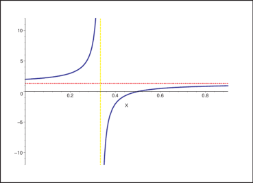
Figure 1: The evolution of $\gamma_{\phi}$ with respect to $X$. The yellow dash vertical line is $X=1/3$, where $\gamma_{\phi}\rightarrow\pm\infty$. The red dash horizontal line is $\gamma_{\phi}=4/3$, $\gamma_{\phi}\rightarrow 4/3$ when $X\rightarrow\infty$. $0\leq\gamma_{\phi}\leq 4/3$ is required from the classical and quantum stabilities.

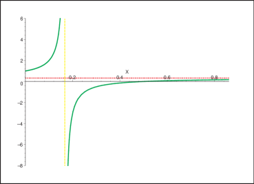
Figure 2: The evolution of $c_{s}^{2}$ with respect to $X$. The yellow dash vertical line is $X=1/6$, where $c_{s}^{2}\rightarrow\pm\infty$. The red dash horizontal line is $c_{s}^{2}=1/3$, $c_{s}^{2}\rightarrow 1/3$ when $X\rightarrow\infty$.

4 Critical Points and their Cosmological Properties

We will investigate the critical points and their properties in this section. The critical points can be found by setting $d\Omega_{\phi}/dN=d\gamma_{\phi}/dN=d\lambda/dN=0$ while their properties are determined by the eigenvalues of the Jacobi matrix ${\cal A}$ of the three dimensional nonlinear autonomous system Eqs.(5, 6, 11). The Jacobi matrix ${\cal A}$ of each point is obtained by linearizing the three dimensional nonlinear autonomous system Eqs.(5, 6, 11) around each critical point[17],

$${\cal A}^{\S}=\left[\begin{array}[]{lll}\partial f_{1}(\Omega_{\phi},\gamma_{\phi},\lambda)/\partial\Omega_{\phi}&\partial f_{1}(\Omega_{\phi},\gamma_{\phi},\lambda)/\partial\gamma_{\phi}&\partial f_{1}(\Omega_{\phi},\gamma_{\phi},\lambda)/\partial\lambda\\ \partial f_{2}(\Omega_{\phi},\gamma_{\phi},\lambda)/\partial\Omega_{\phi}&\partial f_{2}(\Omega_{\phi},\gamma_{\phi},\lambda)/\partial\gamma_{\phi}&\partial f_{2}(\Omega_{\phi},\gamma_{\phi},\lambda)/\partial\lambda\\ \partial f_{3}(\Omega_{\phi},\gamma_{\phi},\lambda)/\partial\Omega_{\phi}&\partial f_{3}(\Omega_{\phi},\gamma_{\phi},\lambda)/\partial\gamma_{\phi}&\partial f_{3}(\Omega_{\phi},\gamma_{\phi},\lambda)/\partial\lambda\end{array}\right]_{each~{}critical~{}point}$$ (13)

Critical point 1(hereafter cp1): $(\Omega_{\phi}=0,\gamma_{\phi}=0,\lambda=\lambda_{ar})$($\lambda_{ar}$ means an arbitrary real constant). Cp1 always exists independent of the form of the potential. It is a barotropic fluid dominated solution. However, since the eigenvalues of cp1 found from its Jacobi matrix is $(3\gamma_{b}/2,-3,0)$, so it is an unstable saddle point.

Critical point 2 (hereafter cp2): $(\Omega_{\phi}=0,\gamma_{\phi}=2,\lambda=\lambda_{ar})$. This point actually does not exist since $\gamma_{\phi}=2>4/3$.

Critical point 3(hereafter cp3): $(\Omega_{\phi}=0,\gamma_{\phi}=4/3,\lambda=\lambda_{ar})$. This point always exists independent of the form of the potential. It is also a barotropic fluid dominated solution. The eigenvalues of cp3 is $(3\gamma_{b}/2-2,1,0)$, so it is an unstable saddle point(for barotropic fluid being matter, $\gamma_{b}=1$) or an unstable node point(for barotropic fluid being radiation, $\gamma_{b}=4/3$).

Critical point 4(hereafter cp4): $(\Omega_{\phi}=1,\gamma_{\phi}=4/3,\lambda=\lambda_{ar})$. This point always exists independent of the form of the potential. cp4 is a power-law kinetic quintessence dominated solution$(\Omega_{\phi}=1)$ where this scalar field behaves as radiation$(\gamma_{\phi}=4/3)$. However, it is an unstable node point(whatever barotropic fluid is matter or radiation) since the eigenvalues of cp4 is $(4-3\gamma_{b},1,0)$.

Critical point 5(hereafter cp5): $(\Omega_{\phi}=1,\gamma_{\phi}=2,\lambda_{1})$, where $\lambda_{1}=0$ or $f(\lambda_{1})=0$. However, this point does not exist since the value of $\gamma_{\phi}$ should be $0\leq\gamma_{\phi}<4/3$.

Critical point 6(hereafter cp6): $(\Omega_{\phi}=1,\gamma_{\phi}=0,\lambda=0)$. This point exists depending on the form of the potential. All the potentials with $\lambda$ being zero in function $f(\lambda)$ have cp6. For example, $f(\lambda)=\beta\lambda-\frac{1}{2}$, the corresponding potential has an implicit expression as $2\beta V(\phi)^{-\frac{1}{2}}-\frac{1}{2}c_{1}ln(V(\phi))=-\frac{1}{2}\kappa\phi+c_{2}$[18]. However, for the potential $V(\phi)=V_{0}/(\phi^{2}-\phi_{0}^{2})$, there is no such critical point since $f(\lambda)=1/2-2/(V_{0}\kappa^{2}\lambda^{2})$, therefore $\lambda$ can not be zero. For the potentials with an extremum(i.e., $V^{\prime}=0$, for example, $V(\phi)=m\phi^{2}/2+V_{0}$) also possess this critical point since the potential related parameter $\lambda=V^{\prime}/(\kappa V^{3/2})$. Cp6 is very interesting since it corresponds to the universe dominated by the dark energy which behaves as an cosmological constant with the sound speed $c_{s}^{2}$ being 0. Furthermore, cp6 could be a stable point since the eigenvalues of this point is $(-3\gamma_{b},-3,0)$. If a critical point of a linear three dimensional dynamical system has the eigenvalues $(-3\gamma_{b},-3,0)$, we can state directly that it is a stable point even though one of the eigenvalues equals zero. However, the dynamical system Eqs.(5,6, 11) in our paper is a nonlinear system, the eigenvalues $(-3\gamma_{b},-3,0)$ is not enough to determine its stability[36]. We need to pursue the stable condition using center manifold theorem[17, 36]. Appendix gives the detailed process to find the stable condition using the center manifold theorem. We find that the stable condition for cp6 is $f(\lambda)|_{\lambda=0}<0$, i.e., $f(0)<0$.

Critical point $7$(hereafter cp$7$): $(\Omega_{\phi}=1,\gamma_{\phi}=-(3\lambda_{\ast}^{3}\pm\lambda_{\ast}\sqrt{9\lambda_{\ast}^{2}+48}),\lambda=\lambda_{\ast})$

Critical point $7_{1}$(hereafter cp$7_{1}$): $(\Omega_{\phi}=1,\gamma_{\phi}=-(3\lambda_{\ast}^{3}+\lambda_{\ast}\sqrt{9\lambda_{\ast}^{2}+48}),\lambda=\lambda_{\ast})$, where $\lambda_{\ast}$ makes $f(\lambda_{\ast})=0$. When $-0.508\leq\lambda_{\ast}\leq 0$, we have $0\leq\gamma_{\phi}<2/3$(see Fig.4), so it is the condition for accelerating expansion. This critical point exist for all the potentials with their $f(\lambda_{\ast})=0$. The simplest case is the inverse square potential $V(\phi)\propto\phi^{-2}$, which is considered in two dimensional system. However, there are many potentials with their $f(\lambda)$ could be zero, the inverse square potential $V(\phi)\propto\phi^{-2}$ is just the simplest case. We can take $V(\phi)=V_{0}/(\phi^{2}-\phi_{0}^{2})$ corresponding to $f(\lambda)=1/2-2/(V_{0}\kappa^{2}\lambda^{2})$[18] as an example. $\lambda_{\ast}=\pm 2/(\kappa\sqrt{V_{0}})$ when $f(\lambda_{\ast})=0$. That means all the critical points exist for inverse square potential will also exist for the potential $V(\phi)=V_{0}/(\phi^{2}-\phi_{0}^{2})$. However, these critical points will not exist for the exponential potential $V(\phi)=V_{0}e^{\alpha\phi}$ since in this case $f(\lambda)$ always equals $-1/2$. The value of $\gamma_{\phi}$ and the eigenvalues of this critical point is quite complicated, we will give its existence and stable condition using numerical analysis. Considering the constraint Eq.(12) from the requirements of the classical and quantum stabilities, the existence condition is $-0.842<\lambda_{\ast}\leq 0$. The stable condition is $-0.662\leq\lambda_{\ast}\leq 0$ and $df_{\lambda_{\ast}}<0$ for both $\gamma_{b}=1$ and $\gamma_{b}=4/3$, where $df_{\lambda_{\ast}}$ is the value of $df(\lambda)/d\lambda|_{\lambda_{\ast}}$. We found that the condition for accelerating expansion $-0.508\leq\lambda_{\ast}\leq 0$ lies in the range of stable condition, therefore the accelerating expansion could be a stable solution.

Critical point $7_{2}$(hereafter cp$7_{2}$): $(\Omega_{\phi}=1,\gamma_{\phi}=-(3\lambda_{\ast}^{3}-\lambda_{\ast}\sqrt{9\lambda_{\ast}^{2}+48}),\lambda=\lambda_{\ast})$. When $-1.923\leq\lambda_{\ast}\leq-1.692$ or $0\leq\lambda_{\ast}\leq 0.689$ or $1.247\leq\lambda_{\ast}\leq 1.692$, we have $0\leq\gamma_{\phi}<2/3$(see Fig.4), so it is the condition for accelerating expansion. The existence condition is $-2.095\leq\lambda_{\ast}\leq-1.692$ or $0\leq\lambda_{\ast}\leq 1.692$. If $\gamma_{b}=1$, the stable condition is $-2.014\leq\lambda_{\ast}\leq-1.692~{}and~{}df_{\lambda_{\ast}}<0$ or $0\leq\lambda_{\ast}\leq 0.328~{}and~{}df_{\lambda_{\ast}}<0$. If $\gamma_{b}=4/3$, the stable condition is $-2.065\leq\lambda_{\ast}\leq-1.692~{}and~{}df_{\lambda_{\ast}}<0$ or $0\leq\lambda_{\ast}\leq 0.328~{}and~{}df_{\lambda_{\ast}}<0$. We found the range of the accelerating condition is overlapped with the stable condition, so cp$7_{2}$ could be a stable accelerating expansion solution. The condition for a stable solution with an accelerating expansion is as follows: $-1.923\leq\lambda_{\ast}\leq-1.692~{}and~{}df_{\lambda_{\ast}}<0$ or $0\leq\lambda_{\ast}\leq 0.328~{}and~{}df_{\lambda_{\ast}}<0$.

The property of cp$7_{2}$ is very similar to cp$7_{1}$, we therefore refer to cp$7$ as cp$7_{1}$ and cp$7_{2}$. We are very interested in these two points since they both could be a stable solution with $\Omega_{\phi}=1$ and $w_{\phi}$ being any value between $-1$ and $-1/3$. Both cp6 and cp$7$ could be a stable solution with dark energy dominating our universe. However cp$7$ is more interesting than cp6 since the state equation $w_{\phi}$ of cp$7$ could be any value between $-1$ and $-1/3$. We find that there is no overlap among the existence condition of cp6, cp$7_{1}$ and cp$7_{2}$, so they will not exist simultaneously.

Critical point $8$(hereafter cp$8$): $(\Omega_{\phi}=3\gamma_{b}^{2}/[(4-3\gamma_{b})\lambda_{\ast}^{2}],\gamma_{\phi}=\gamma_{b},\lambda=\lambda_{\ast})$, where $\lambda_{\ast}$ makes $f(\lambda_{\ast})=0$. This critical point exist for all the potentials with their $f(\lambda_{\ast})=0$, similar to the critical points cp$7_{1}$ and cp$7_{2}$. If barotropic fluid is radiation(i.e., $\gamma_{b}$=4/3), cp$8$ have no meaning since $\Omega_{\phi}=3\gamma_{b}^{2}/[(4-3\gamma_{b})\lambda_{\ast}^{2}]\rightarrow\infty$^‡. So here barotropic fluid could only be matter(i.e., $\gamma_{b}$=1), then $\Omega_{\phi}=3/\lambda_{\ast}^{2}$, we therefore obtain $|\lambda_{\ast}|\geq\sqrt{3}$ to make $\Omega_{\phi}\leq 1$. The stable condition for this scaling solution is $\lambda_{\ast}\leq-\sqrt{3}$ and $df_{\lambda_{\ast}}<0$(stable node for $-2\sqrt{2}\leq\lambda_{\ast}\leq-\sqrt{3}$ and stable spiral for $\lambda_{\ast}<-2\sqrt{2}$). Cp$8$ is the scaling solution where neither the scalar field nor the ordinary matter entirely dominates the universe. The scalar field behaves as the ordinary matter in this case.

5 Discussions and Conclusions

We have found all the critical points of three dimensional dynamical nonlinear autonomous system of power-law kinetic quintessence, given their existence and stable conditions and analyzed their cosmological implications in section 4. Here we will give the discussions and conclusions about their cosmological implications.

There are totally eight critical points for the dynamical system Eqs.(5, 6, 11), but only six critical points(cp$1$, cp$3$, cp$4$, cp$6$ ,cp$7$, cp$8$) exist if the classical and quantum stability was considered. Among these critical points, cp$1$, cp$3$ and cp$4$ always exist and are independent of the form of the potentials. However, all of these critical points which are independent of potentials are unstable. cp$1$ is an unstable saddle point while cp$4$ is an unstable node. cp$3$ is quite special since it is an unstable saddle point when $\gamma_{b}=1$(matter) and an unstable node point when $\gamma_{b}=4/3$(radiation). From a mathematical point of view, the unstable node is different from the unstable saddle. All the trajectories of an unstable node will move away from the critical point to infinite-distant away while some trajectories of a saddle are drawn to the critical point and other trajectories recede. So the unstable node and saddle actually have different cosmological implication even though they are all unstable.

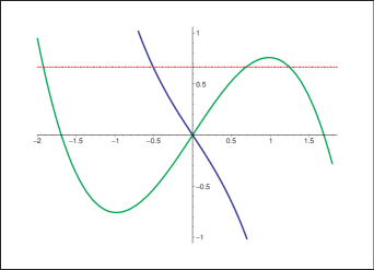
Figure 3: The evolution of $\gamma_{\phi}$ with respect to $\lambda_{\ast}$. Blue line is for cp$7_{1}$ with $\gamma_{\phi}=-(3\lambda_{\ast}^{3}+\lambda_{\ast}\sqrt{9\lambda_{\ast}^{2}+48})$ while solid line is for cp$7_{2}$ with $\gamma_{\phi}=-(3\lambda_{\ast}^{3}-\lambda_{\ast}\sqrt{9\lambda_{\ast}^{2}+48})$. Red dash horizontal line is $\gamma_{\phi}=2/3$. $0\leq\gamma_{\phi}\leq 2/3$ is required for the accelerating expansion of universe.

Figure 4: The evolution of the sound speed $c_{s}^{2}$ with respect to $\gamma_{\phi}$. Blue line is for power-law kinetic quintessence($c_{s}^{2}=-\gamma_{\phi}/(3\gamma_{\phi}-8)$), where $c_{s}^{2}$ is monotonically increasing from $0$ to $1/9$ when $\gamma_{\phi}$ varies from $0$ to $2/3$. Red line is for quintessence($c_{s}^{2}=1$), green line is for tachyon($c_{s}^{2}=1-\gamma_{\phi}$).

The existence of other three critical points cp$6$, cp$7$ and cp$8$ depend on the form of the potentials. It is very interesting that all these three critical points could be stable points if some conditions are satisfied. Cp$6$ exists when the potential related parameter $\lambda$ could be $0$ in the function $f(\lambda)$. Cp$7$ and cp$8$ exists when $f(\lambda)$ could be $0$. These three critical points cp$6$, cp$7$ and cp$8$ have more important cosmological implication than cp$1$, cp$3$ and cp$4$. Cp$6$ is a new critical point which is found only in three dimensional dynamical system. Cp$6$ corresponds to the dark energy dominated universe($\Omega_{\phi}=1$) where power-law kinetic quintessence behaves as an cosmological constant with the sound speed $c_{s}^{2}$ being 0. So cp$6$ is a little different from canonical quintessence and tachyon model since $c_{s}^{2}=1$ for both of those scalar field. Cp$7$ and cp$8$ correspond to the famous dominant and scaling attractors respectively which are also found in quintessence model[17, 37] and tachyon model[18, 19]. Similar to cp$6$, cp$7$ is also a dark energy dominated attractors ($\Omega_{\phi}=1$). However, cp$7$ is different from cp$6$ on two points. The first difference is that cp$7$ is not a de-Sitter-like dominant attractor since the state equation $w_{\phi}$ of cp$7$ could be any value between $-1$ and $-1/3$(see Fig.4, note that $0\leq\gamma_{\phi}=w_{\phi}+1\leq 2/3$) depending on the different value of $\lambda_{\ast}$. So the value of state equation of dark energy $w_{\phi}$ could be matched to the value from the observational data. The second difference is that the sound speed $c_{s}^{2}$ is monotonically increasing with $\gamma_{\phi}$ instead of being zero(see Fig.4). cp$8$ is the scaling solution that power-law kinetic quintessence will track the evolution of background matter in the early time and behaves as the ordinary matter with $\Omega_{\phi}=3/\lambda_{\ast}^{2}$ and $\gamma_{\phi}=1$. We proved in section 4 that this scaling is only possible for ordinary matter($\gamma_{b}=1$), which is different from the result obtained in quintessence model[17, 37].

Though the existence and stable conditions are different for cp$6$, cp$7$ and cp$8$, it is very interesting to consider the possibility that our universe may evolve continuously from one stable critical point(cp$8$, scaling solution) to another stable one(cp$6$ or cp$7$, dark energy dominant solution). We borrow the idea in Ref[20] where the author proposed a scenario of universe which could evolve from a scaling attractor to another dark energy dominant attractor by introducing a field whose value changed by a certain amount in a short time. Since the change of the value of scalar field $\phi$ means the change of the value of $\lambda_{\ast}$, then cp$6$, cp$7$ and cp$8$ could be stable before and after the change of scalar field $\phi$. Actually, we can also obtain these two asymptotical evolutions if the potential $V(\phi)$ can be approximated to two different potentials when scalar field $\phi$ evolves into different ranges: one admits the scaling solution and another admits the dark energy dominant solution[38, 39, 40]. For these potentials, the exit of the cosmological evolution from one attractor solution to another attractor is quite natural, but the explanation of why we have these special potentials may require fine tuning.

In the end of this paper, we would like to discuss cp$7$ and cp$8$ from the observational point of view. The sound speed $c_{s}^{2}$ in the case of cp$7$ and cp$8$ is very special comparing to other scalar field models, which makes it possible to distinguish the power-law kinetic quintessence from other scalar field models using the observational data. The sound speed $c_{s}^{2}$ of cp$7$ is monotonically increasing with $\gamma_{\phi}$ instead of being zero. We can see from Fig.4 that $0\leq c_{s}^{2}\leq 1/9$ when $0\leq\gamma_{\phi}\leq 2/3$, and the closer $w_{\phi}$ is to $-1$, the closer $\gamma_{\phi}$ is to $0$. We also plot the relationship between $c_{s}^{2}$ and $\gamma_{\phi}$ of canonical quintessence and tachyon in Fig.4 for comparing with each other. We can find that the value of $c_{s}^{2}$ of power-law kinetic quintessence is dramatically less than the sound speed of canonical quintessence and tachyon. Since the nature of dark energy can be probed not only through $w_{\phi}$ but also through its microphysics, characterized by the sound speed of perturbations to the dark energy density and pressure. As the sound speed $c_{s}^{2}$ drops below the speed of light, dark energy inhomogeneities increase, affecting both cosmic microwave background and matter power spectra[12, 41]. It is shown that observational data may distinguish the dark energy models with the sound speed $c_{s}^{2}\ll 1$ from the models with $c_{s}^{2}\rightarrow 1$[13, 42, 43, 44, 45, 46], so in principle it could be distinguished from canonical quintessence and tachyon(see Fig.4). For the case of cp$8$, power law kinetic quintessence behaves as ordinary matter with $\gamma_{\phi}=1$. For the ordinary matter(or dark matter), we know that $c_{s}^{2}=0$. However, it is very interesting to notice here that the sound speed $c_{s}^{2}$ equals $1/5$ from Eq.(9). It means that power-law kinetic quintessence track the evolution of ordinary matter with the same state equation $w_{m}$ but a different sound speed $c_{s}^{2}$. This is very important since the behavior of perturbation in scalar field dark energy and its consequent effect on the cold dark matter power spectrum is governed by the state equation $w_{\phi}$ and the effective speed of sound $c_{s}^{2}$ of dark energy. For the scaling solution cp$8$, the dark energy density was non-negligible($\Omega_{\phi}=3/\lambda_{\ast}^{2}\neq 0$) at early times(Early Dark Energy models[47]). It is shown that as $\gamma_{\phi}$ gets further from 0, the influence of the sound speed increases; for models with $\gamma_{\phi}\approx 1$ at high redshift there is also the possibility of non negligible amounts of early dark energy density. So even just a couple percent of the total energy density in early dark energy can dramatically improve the prospects for detecting dark energy clustering[41]. The impact of early dark energy fluctuations in both linear and nonlinear regimes of structure formation had been explored in Ref[48]. In these models the energy density of dark energy is non-negligible at high redshift and the fluctuations in the dark energy component can have the same order of magnitude of dark matter fluctuations. However, how the impact will be changed if the $c_{s}^{2}$ equals $1/5$ for power-law kinetic quintessence is not investigated yet. Since power-law kinetic quintessence are special both in the early universe where it is an early dark energy tracking the ordinary matter with $c_{s}^{2}=1/5$ and in the late universe where it drives the accelerating expansion with $c_{s}^{2}\rightarrow 0$, it may be a good suggestion to simultaneously investigate the perturbations of dark energy at both early and late time universe, and to explore whether there are any degeneracies of the impacts between early dark energy and late dark energy on cold dark matter power spectrum and cosmic microwave background.

6 Acknowledgement

This work is partly supported by National Nature Science Foundation of China under Grant No. 11333001, Shanghai Research Grant No. 13JC1404400 and Shanghai Normal University Research Program under Grant No. SK201309.

Appendix

In section 4, we pointed out that if the eigenvalues of Jacobi matrix has one or more eigenvalues with zero real parts while the rest of the eigenvalues are negative, then linearization fails to determine the stability properties of this critical point. Among the six critical points(cp$1$, cp$3$, cp$4$, cp$6$ ,cp$7$, cp$8$) investigated in this paper, cp6 is just such point. So in this Appendix we will show you how we get the stable condition of cp6 using the center manifold theorem[36]. The point cp6 is: $(\Omega_{\phi},\gamma_{\phi},\lambda)=(1,0,0)$, and its three eigenvalues are $-3\gamma_{b}$, $-3$ and $0$. Firstly, we need to transfer cp6 to $cp6^{\prime}$ $(\Omega_{1}=\Omega_{\phi}-1,\gamma_{\phi},\lambda)=(0,0,0)$ for convenience. In this case, Eqs.(5, 6, 11) can be rewritten as:

$$\frac{d\Omega_{1}}{dN}=-3(\gamma_{b}-\gamma_{\phi})\Omega_{1}(\Omega_{1}+1)$$ (14)

$$\frac{d\gamma_{\phi}}{dN}=\frac{(\lambda\sqrt{3(4-3\gamma_{\phi})(\Omega_{1}+1)}+3\gamma_{\phi})(\gamma_{\phi}-2)(3\gamma_{\phi}-4)}{3\gamma_{\phi}-8}$$ (15)

$$\frac{d\lambda}{dN}=\lambda^{2}\sqrt{3(4-3\gamma_{\phi})(\Omega_{1}+1)}~{}f(\lambda)$$ (16)

Noted that now $\Omega_{1}$, $\gamma_{\phi}$, $\lambda$ in Eqs.(14, 15, 16) are very small variables around $cp6^{\prime}$ ($\Omega_{1}=0,\gamma_{\phi}=0,\lambda=0$). Function $f(\lambda)$ in Eq.(14) could be taken the taylor series in $\lambda$: $f(\lambda)=f(0)+f^{1}(0)\lambda+\frac{f^{2}(0)}{2!}\lambda^{2}+...$, where $f^{n}(0)$ is the value of $\frac{d^{n}f(\lambda)}{d\lambda^{n}}$ when $\lambda=0$.

We get the Jacobi matrix ${\cal A}$ of nonlinear autonomous dynamical system Eqs.(14, 15, 16) from Eq.(13):

$${\cal A}=\left[\begin{array}[]{lll}-3\gamma_{b}&\ \ 0&\ \ \ \ 0\\ \ \ 0&-3&\ \ -2\sqrt{3}\\ \ \ 0&\ \ 0&\ \ \ \ 0\end{array}\right]$$ (17)

The eigenvalues of ${\cal A}$ and the corresponding eigenvectors are:

$$\{-3\gamma_{b},\ \ [1,0,0]\};\ \ \ \ \ \{-3,\ \ [0,1,0]\};\ \ \ \ \ \{0,\ \ [0,-\frac{2}{\sqrt{3}},1]\}$$ (18)

Let ${\cal M}$ be a matrix whose columns are the eigenvectors of ${\cal A}$, then we can write down ${\cal M}$ and its inverse matrix ${\cal T}$:

$${\cal M}=\left[\begin{array}[]{lll}\ 1&\ 0&\ \ 0\\ \ 0&\ 1&-\frac{2}{\sqrt{3}}\\ \ 0&\ 0&\ \ 1\end{array}\right],\ \ \ \ \ \ {\cal T}={\cal M}^{-1}=\left[\begin{array}[]{lll}\ 1&\ 0&\ \ 0\\ \ 0&\ 1&\frac{2}{\sqrt{3}}\\ \ 0&\ 0&\ \ 1\end{array}\right]$$ (19)

Using the similarity transformation ${\cal T}$ we can transform ${\cal A}$ into a block diagonal matrix, that is,

$${\cal T}{\cal A}{\cal T}^{-1}=\left[\begin{array}[]{lll}-3\gamma_{b}&\ 0&\ \ 0\\ \ \ 0&-3&\ \ 0\\ \ \ 0&\ 0&\ \ 0\end{array}\right]=\left[\begin{array}[]{ll}{\cal A}_{1}&\ 0\\ 0&{\cal A}_{2}\end{array}\right]$$ (20)

where all eigenvalues of ${\cal A}_{1}$ have negative real parts while eigenvalue of ${\cal A}_{2}$ has zero real part. We then change the variables ($\Omega_{1},\gamma_{\phi},\lambda$) in Eqs.(14, 15, 16) to another set ($\Omega_{2},\gamma_{1},\lambda_{1}$) as follows:

$$\left[\begin{array}[]{l}\Omega_{2}\\ \gamma_{1}\\ \lambda_{1}\end{array}\right]={\cal T}\left[\begin{array}[]{l}\Omega_{1}\\ \gamma_{\phi}\\ \ \lambda\end{array}\right]=\left[\begin{array}[]{l}\ \ \ \Omega_{1}\\ \gamma_{\phi}+\frac{2}{\sqrt{3}}\lambda\\ \ \ \ \ \lambda\end{array}\right]$$ (21)

Then we can rewrite the dynamical system Eqs.(14, 15, 16) in the form of the new variables:

$$\frac{d\Omega_{2}}{dN}=\frac{d\Omega_{1}}{dN}=-3(\gamma_{b}-\gamma_{1}+\frac{2}{\sqrt{3}}\lambda_{1})(\Omega_{2}+1)\Omega_{2}=G_{1}(\Omega_{2},\gamma_{1},\lambda_{1})$$ (22)

$$\frac{d\gamma_{1}}{dN}=\frac{d\gamma_{\phi}}{dN}+\frac{2}{\sqrt{3}}\frac{d\lambda}{dN}=2\lambda_{1}^{2}\sqrt{(4-3\gamma_{1}+2\sqrt{3}\lambda_{1})(\Omega_{2}+1)}f(\lambda_{1})$$

$$+\frac{(\lambda_{1}\sqrt{3(4-3\gamma_{1}+2\sqrt{3}\lambda_{1})(\Omega_{2}+1)}+3\gamma_{1}-2\sqrt{3}\lambda_{1})(\gamma_{1}-\frac{2}{\sqrt{3}}\lambda_{1}-2)(3\gamma_{1}-2\sqrt{3}\lambda_{1}-4)}{3\gamma_{1}-2\sqrt{3}\lambda_{1}-8}=G_{2}(\Omega_{2},\gamma_{1},\lambda_{1})$$ (23)

$$\frac{d\lambda_{1}}{dN}=\frac{d\lambda}{dN}=\lambda_{1}^{2}\sqrt{3(4-3\gamma_{1}+2\sqrt{3}\lambda_{1})(\Omega_{2}+1)}~{}f(\lambda_{1})=G_{3}(\Omega_{2},\gamma_{1},\lambda_{1})$$ (24)

According to the center manifold theorem, the stable properties of cp6 is determined by reduced system Eq.(24). We set the center manifold for $\Omega_{2}$ and $\gamma_{1}$:

$$\Omega_{2}=h_{1}(\lambda_{1});\ \ \ \ \ \gamma_{1}=h_{2}(\lambda_{1})$$ (25)

where $h_{1},h_{2}$ are the function of $\lambda_{1}$ which satisfy following conditions:

$$h_{1}(0)=0;\ \ \frac{\partial h_{1}}{\partial\lambda_{1}}=0;\ \ \ \ h_{2}(0)=0;\ \frac{\partial h_{2}}{\partial\lambda_{1}}=0$$ (26)

The center manifold equations are as follows:

$$G_{1}(h_{1}(\lambda_{1}),h_{2}(\lambda_{1}),\lambda_{1})=\frac{\partial h_{1}}{\partial\lambda_{1}}\cdot G_{3}(h_{1}(\lambda_{1}),h_{2}(\lambda_{1}),\lambda_{1})$$ (27)

$$G_{2}(h_{1}(\lambda_{1}),h_{2}(\lambda_{1}),\lambda_{1})=\frac{\partial h_{2}}{\partial\lambda_{1}}\cdot G_{3}(h_{1}(\lambda_{1}),h_{2}(\lambda_{1}),\lambda_{1})$$ (28)

We set $h_{1}=a_{2}\lambda_{1}^{2}+a_{3}\lambda_{1}^{3}+\cdots,h_{2}=b_{2}\lambda_{1}^{2}+b_{3}\lambda_{1}^{3}+\cdots$ and substitute these series into the center manifold equations Eqs.(27, 28) to find the unknown coefficients $a_{2},b_{2},a_{3},b_{3},\cdots$ by matching the coefficients of like powers in $\lambda_{1}$ in the left and right sides of equations Eqs.(27, 28). However, we do not know in advance how many terms of the series of $h_{1},h_{2}$ we need. We start with the simple approximation: $h_{1}=a_{2}\lambda_{1}^{2}+a_{3}\lambda_{1}^{3},h_{2}=b_{2}\lambda_{1}^{2}+b_{3}\lambda_{1}^{3}$, and get that $a_{2}=a_{3}=0$, $b_{2}=-\frac{1}{2}+\frac{4}{3}f(0)$, $b_{3}=\frac{4}{3}f^{1}(0)+\frac{5}{9}\sqrt{3}f(0)-\frac{\sqrt{3}}{16}-\frac{16}{9}\sqrt{3}f(0)^{2}$. We therefore set $h_{1}=a_{4}\lambda_{1}^{4}+a_{5}\lambda_{1}^{5}+a_{6}\lambda_{1}^{6}+a_{7}\lambda_{1}^{7}$, and found $a_{4}=a_{5}=a_{6}=a_{7}=0$. So we finally set $h_{1}=0$, $h_{2}=[-\frac{1}{2}+\frac{4}{3}f(0)]\lambda_{1}^{2}+[\frac{4}{3}f^{1}(0)+\frac{5}{9}\sqrt{3}f(0)-\frac{\sqrt{3}}{16}-\frac{16}{9}\sqrt{3}f(0)^{2}]\lambda_{1}^{3}$.

So we substitute $h_{1},h_{2}$ into the reduced system Eq.(24) and rewrite it as follows:

$$\frac{d\lambda_{1}}{dN}=\lambda_{1}^{2}\sqrt{3}\sqrt{4+2\sqrt{3}\lambda_{1}-[4f(0)-\frac{3}{2}]\lambda_{1}^{2}-[\frac{5}{3}\sqrt{3}f(0)-\frac{16}{3}\sqrt{3}f(0)^{2}+4f^{1}(0)-\frac{3\sqrt{3}}{16}]\lambda_{1}^{3}}~{}f(\lambda_{1})$$ (29)

where $f(\lambda_{1})$ can be expanded as $f(0)+f^{1}(0)\lambda+\cdots$. Since $\lambda_{1}$ is a very small variable around $\lambda_{1}=0$, so Eq.(29) can be simplified in the neighborhood of $\lambda_{1}$ as follows:

$$\frac{d\lambda_{1}}{dN}=2\sqrt{3}f(0)\lambda_{1}^{2}$$ (30)

where $f(0)$ is the value of function $f(\lambda)$ at $\lambda=0$. The stability of cp6 will be finally determined by above simplest reduced system Eq.(30). It is clear that the stable condistion for dynamical system Eq.(30) is

$$f(0)<0$$ (31)

So in this Appendix we proved that cp6 is a stable de-Sitter-like dominant attractor when $f(0)<0$, just as stated in section 4.

References

- [1] C. Armendariz-Picon, T. Damour and V. Mukhanov, Phys. Lett. B458, 209-218 (1999)
- [2] T. Chiba, T. Okabe and M. Yamaguchi, Phys. Rev. D62, 023511 (2000)
- [3] C. Armendariz-Picon, V. Mukhanov and Paul J. Steinhardt, Phys.Rev.D63, 103510 (2001)
- [4] J. P. Ostriker and P. J. Steinhardt, Nature 377, 600 (1995)
- [5] B. P. Schmidt et al., ApJ. 507, 46 (1998)
- [6] A. G. Riess et al., Astron. J. 116, 1009 (1998)
- [7] S. Perlmutter et al., ApJ. 517, 565 (1999)
- [8] R. J. Scherrer, Phys. Rev. Lett.93, 011301 (2004)
- [9] D. Sapone, M. Kunz and L. Amendola, Phys. Rev. D82, 103535 (2010)
- [10] E. Calabrese, R. de Putter, D. Huterer, E.V. Linder and A. Melchiorri, Phys. Rev. D83, 023011 (2011)
- [11] J. K. Erickson, R. R. Caldwell, P. J. Steinhardt, C. Armendriz-Picn, and V. Mukhanov, Phys. Rev. Lett.88, 121301 (2002)
- [12] S. DeDeo, R. R. Caldwell, and P. J. Steinhardt, Phys. Rev. D67, 103509 (2003)
- [13] R. Bean and O. Dor, Phys.Rev.D69, 083503 (2004)
- [14] S. Anselmi, G. Ballesteros and M. Pietroni, JCAP11, 014(2011)
- [15] S. A. Appleby, E. V. Linder and J. Weller, Phys. Rev. D88, 043526 (2013)
- [16] S. Mizuno and K. I. Maeda, Phys.Rev. D64, 123521 (2001)
- [17] W. Fang, Y. Li, K. Zhang and H. Q. Lu, Class. Quantum Grav.26, 155005 (2009)
- [18] W. Fang and H. Q. Lu, Eur. Phys. J. C68, 567-572 (2010)
- [19] J. M. Aguirregabiria and R. Lazkoz, Phys. Rev. D69, 123502 (2004)
- [20] S. Y. Zhou, Phys. Lett. B660, 7-12 (2008)
- [21] W. Fang, H. Tu, J. S. Huang, C. G. Shu, arXiv:1402.4045
- [22] R. J. Yang and X. T. Gao, Class. Quant. Grav.28, 065012 (2011)
- [23] Y. Leyva, D. Gonzalez, T.Gonzalez, T. Matos and I. Quiros, Phys. Rev. D80, 044026 (2009)
- [24] T. Matos, J. R. Luevano, I. Quiros, L. A. Urena-Lopez and J. A. Vazquez, Phys. Rev. D80, 123521 (2009)
- [25] I. Quiros, T. Gonzalez, D. Gonzalez, Y. Napoles, R. Garcia-Salcedo and C. Moreno, Class. Quant. Grav.27, 215021(2010)
- [26] K. Xiao and J. Y. Zhu, Phys. Rev. D83, 083501 (2011)
- [27] D. Escobar, C. R. Fadragas, G. Leon and Y. Leyva, Class. Quantum Grav.29, 175005 (2012)
- [28] D. Escobar, C. R. Fadragas, G. Leon and Y. Leyva, Class. Quantum Grav.29, 175006 (2012)
- [29] G. Leon, Y. Leyva and J. Socorro, arXiv:1208.0061
- [30] S. del Campo, C. R. Fadragas, R. Herrera, C. Leiva, G. Leon and J. Saavedra, Phys. Rev. D88, 023532 (2013)
- [31] G. Otalora, Phys. Rev. D88, 063505 (2013)
- [32] G. Otalora, JCAP07, 044 (2013)
- [33] G. Otalora, arXiv:1402.2256
- [34] F. Piazza and S. Tsujikawa, JCAP0407, 004 (2004)
- [35] A. A. H. Graham and R. Jha, arXiv:1401.8203v1
- [36] H. K. Khalil, Nonlinear Systems, 2nd edn(Englewood Cliffs, NJ: Prentice Hall) pp166-177 (1996)
- [37] E. J. Copeland, A. R. Liddle and D. Wands,Phys. Rev. D57, 4686 (1998)
- [38] T. Barreiro, E. J. Copeland and N. J. Nunes, Phys. Rev. D61, 127301 (2000)
- [39] V. Sahni and L. M. Wang, Phys. Rev. D62, 103517 (2000)
- [40] A. Albrecht and C. Skordis, Phys. Rev. Lett.84,2076 (2000)
- [41] R. de Putter, D. Huterer and E. V. Linder, Phys. Rev. D81, 103513 (2010)
- [42] A. Torres-Rodriguez, C. M. Cress and K. Moodley, MNRAS388, 669-676 (2008)
- [43] G. Ballesteros and J. Lesgourgues, JCAP1010, 014 (2010)
- [44] T. Basse, O. Bjaelde and Yvonne Y. Y. Wong, JCAP1110, 038 (2011)
- [45] T. Basse, O. Bjaelde, S. Hannestad and Yvonne Y. Y. Wong, arXiv:1205.0548
- [46] R. Ul Haq Ansari and S.Unnikrishnan, J. Phys.: Conf. Ser.484, 012048(2014); arXiv:1104.4609
- [47] M. Doran and G. Robbers, JCAP0606, 026 (2006)
- [48] R. C. Batista, F. Pace, JCAP1306, 044 (2013)