Calculation of size for bound-state constituents

Abstract

Elements are given of a calculation that identifies the size of a proton in the Schrödinger equation for lepton-proton bound states, using the renormalization group procedure for effective particles (RGPEP) in quantum field theory, executed only up to the second order of expansion in powers of the coupling constant. Already in this crude approximation, the extraction of size of a proton from bound-state observables is found to depend on the lepton mass, so that the smaller the lepton mass the larger the proton size extracted from the same observable bound-state energy splitting. In comparison of Hydrogen and muon-proton bound-state dynamics, the crude calculation suggests that the difference between extracted proton sizes in these two cases can be a few percent. Such values would match the order of magnitude of currently discussed proton-size differences in leptonic atoms. Calculations using the RGPEP of higher order than second are required for a precise interpretation of the energy splittings in terms of the proton size in the Schrödinger equation. Such calculations should resolve the conceptual discrepancy between two conditions: that the renormalization group scale required for high accuracy calculations based on the Schrödinger equation is much smaller than the proton mass (on the order of a root of the product of reduced and average masses of constituents) and that the energy splittings due to the physical proton size can be interpreted ignoring corrections due to the effective nature of constituents in the Schrödinger equation.

IFT/14/02

I Introduction

The approach suggested here for research on questions concerning the size of a proton in lepton-proton bound states differs from several approaches to bound-state dynamics that are available in the literature BetheSalpeter ; GellMannLow ; BetheSalpeterBook ; CaswellLepage ; KinoshitaQED ; Kinoshita1999 ; PachuckiMuon ; PachuckiAtoms ; Jones2 ; Kinoshita2012 ; Mohr2012 ; radius2013 . The suggested approach is not meant to easily achieve the accuracy that could rival advanced quantitative calculations. Instead, these notes address the conceptual issue of effective nature of constituents in the non-relativistic Schrödinger quantum mechanics.

The constituents seen in bound-states are not considered here the same as the quanta of an underlying theory. They are instead treated as calculable, effective quanta in the renormalized theory. The required method of calculation is the renormalization group procedure for effective particles (RGPEP), whose recent summary can be found in Ref. pRGPEP . The effective particles and their interactions depend on the RGPEP scale parameter. The discussion of the proton size that follows accounts for the presence of such scale parameter in the two-body Schrödinger eigenvalue equation.

The effective nature of the two-body Schrödinger approximation has an implication that the lepton-proton interaction cannot be precisely local. The non-locality is associated with the finite value of the RGPEP scale parameter required to justify the approximation of a bound state in terms of just two constituents in the Schrödinger equation. The range of the non-locality is small in comparison to the distances that characterize dominant effects in the bound-state dynamics. The small non-locality range can be estimated on the general grounds of universality of the Schrödinger equation for systems bound by electromagnetic interactions, using scaling with the fine structure constant $\alpha$. The point of this article is that the non-locality matters in the interpretation of corrections due to the physical proton radius with accuracy comparable to 1%.

The argument presented here is purely heuristic. It is based on a crude estimate of the coefficient, denoted here by $d_{a}$, in front of the proton radius parameter squared, $r_{p}^{2}$, in the ground-state lepton-proton binding energy correction due to the proton radius [cf. Eq. (122) in Sec. V.2],

$$\Delta E_{r} = d_{a}\ {2\pi\alpha\over 3}\ r_{p}^{2}\ |\hat{\psi}(0)|^{2}\ .$$ (1)

The parameter $d_{a}$ must deviate from 1 in an effective theory. The size of deviation depends on the value of the number $a$ which says how much the RGPEP scale parameter $\lambda=1/s$, where $s$ has the interpretation of the size of effective particles, differs from a special value selected on the basis of universality of electric charge and the Schrödinger quantum mechanics. One infers that

$$\lambda = a\ \sqrt{\mu M}\ ,$$ (2)

where $\mu$ is the reduced and $M$ the average mass of constituents in a two-body bound state. With this choice one obtains the bound-state picture that universally scales with $\alpha$ if one uses the same $a$ in different systems. This means that one changes $\lambda$ when masses of the constituents change. On the other hand, when one uses the same $\lambda$ to discuss different systems in one and the same effective theory, one obtains different values of $a$ for different values of the constituent masses.

It follows from Eq. (2) that $a$ is reduced by the factor of about $\sqrt{m_{e}/m_{\mu}}\sim 14$ when one goes from the muon-proton to electron-proton system without changing $\lambda$ in the effective theory. The associated change in the coefficient $d_{a}$ in Eq. (1) can reach the unexpectedly large values such as 8%. The surprise comes from the fact that the corrections result from a non-perturbative factor that, when formally expanded in powers of $\alpha$, appears to correspond to corrections order $\alpha^{4}\sim 10^{-9}$ to Rydberg. The expansion is not valid, however, due to the ultraviolet divergences it illegitimately creates. On the other hand, without taking into account the non-perturbative result that $d_{a}\neq 1$ in Eq. (1), one might have an impression that the proton radius could be greater in the electron-proton system by about 4% than in the muon-proton system.

The possibility of obtaining an effect on the order of a few percent in the proton radius extracted from one term in a theory of energy splittings does not mean that the proton radius puzzle is explained. On the contrary, this finding provides evidence that the effective nature of Schrödinger picture for lepton-proton bound states must be brought under mathematical control as a function of the relevant scale parameter before one can arrive at firm conclusions. In exact calculations, observables cannot depend on the choice of scale for effective theory. But when one relies on approximations and one is not in possession of mathematical control over the effective theory dependence on the scale parameter, an artificial dependence of the proton radius on the system it is extracted from cannot be excluded. The RGPEP appears to be a candidate for attempts to remove this ambiguity and to compare the underlying theory with data including the proton radius effects.

These notes start with an introduction of the proton radius in Sec. II. The effective nature of the Schrödinger equation is discussed in Sec. III, illustrated by a derivation in Sec. IV. The effective size of the proton is considered in Sec. V and Sec. VI concludes the notes. Appendix A shows an example of construction of a canonical Hamiltonian. An outline of the RGPEP is given in App. B. Details of the effective lepton-proton interaction are discussed in App. C and a few details concerning evaluation of $d_{a}$ are given in App. D.

II Proton size in quantum mechanics

In the instant form (IF) of Hamiltonian dynamics DiracFF , the effective proton size in lepton-proton bound states can be introduced using the non-relativistic Schrödinger equation,

$${\vec{p}^{\,2}\over 2\mu}\,\psi(\vec{p}\,)+\int{d^{3}k\over(2\pi)^{3}}\,V(\vec{p},\vec{k}\,)\,\psi(\vec{k}\,) = -E_{B}\,\psi(\vec{p}\,)\ ,$$ (3)

where the kernel $V(\vec{p},\vec{k}\,)$ describes the interaction, $\vec{k}$ and $\vec{p}$ denote the relative momenta in the lepton-proton center-of-mass system before and after the interaction, $\mu$ is the reduced mass, and $E_{B}$ is the binding energy, which is defined as the difference between the sum of the constituent masses, expressed here by the average mass $M$,

$$m_{l}+m_{p} = 2M\ ,$$ (4)

and the bound-state mass $M_{B}$,

$$M_{B} = 2M-E_{B}\ .$$ (5)

In the first approximation for lepton-proton bound states, $V(\vec{p},\vec{k}\,)$ is equal to the spin-independent Coulomb potential for point-like charges, $V^{\rm pt}_{C}(\vec{q}\,)$, where $\vec{q}=\vec{p}-\vec{k}$ and

$$V^{\rm pt}_{C}(\vec{q}\,) = -\ {4\pi\alpha\over\vec{q}^{\,2}}\,.$$ (6)

In this approximation, the proton size can be accounted for by the replacement of $V^{\rm pt}_{C}$ with

$$V_{C}(\vec{q}\,) = V^{\rm pt}_{C}(\vec{q}\,)\ G_{E}(\vec{q}\,^{2})\ ,$$ (7)

where $G_{E}$ denotes the proton electric form factor, cf. Eq. (2) in Ref. radius2013 .

The proton radius, denoted by $r_{p}$, enters in the interaction $V(\vec{p},\vec{k}\,)$ in a known way because the momentum transfers $\vec{q}$ between constituents in the lepton-proton bound states are small in comparison with the inverse of the proton size and the proton form-factor dependence on such small momentum transfers is described by the formula

$$G_{E}(\vec{q}\,^{2})=1-{1\over 6}\,r_{p}^{2}\,\vec{q}\,^{2}+o(\vec{q}\,^{2})\ .$$ (8)

Thus, the interaction can be approximated by

$$V_{C}(\vec{q}\,) = V^{\rm pt}_{C}(\vec{q}\,)+{2\pi\alpha\over 3}\,r_{p}^{2}\ .$$ (9)

In position variables,

$$V_{C}(\vec{r}\,) = -{\alpha\over|\vec{r}\,|}+{2\pi\alpha\over 3}\,r_{p}^{2}\ \delta^{3}(\vec{r}\,)\ .$$ (10)

Since the parameter $r_{p}$ is meant to describes a physical feature of the proton radius2010e , there is no obvious reason to expect that $r_{p}$ differs in the electron-proton and muon-proton bound states.

However, splittings in the muon-proton bound-state spectra are measured with accuracy much better than the magnitude of corrections caused by the term

$$\delta V(\vec{p},\vec{k}\,) = {2\pi\alpha\over 3}\,r_{p}^{2}\ ,$$ (11)

or, in its position representation,

$$\delta V(\vec{r}\,) = {2\pi\alpha\over 3}\,r_{p}^{2}\ \delta^{3}(\vec{r}\,)\ .$$ (12)

Differences between observed splittings in the spectra of electron-proton and muon-proton bound states radius2010a can be interpreted, including insight from Eqs. (11) and (12), as resulting from $r_{p}$ being about 4% greater in the electron-proton bound states than in the muon-proton bound states radius2013 . While the available data suggest this interpretation, it is difficult to explain variation of the proton radius in theory. Therefore, the 4% difference is called the proton radius puzzle.

We suggest that a resolution of the proton radius puzzle may originate in details of the relationship between the Schrödinger equation, Eq. (3), and quantum field theory (QFT). Namely, one needs to precisely define the steps through which the complex bound-state dynamics of relativistic QFT is reduced to a non-relativistic equation for the two particles that interact with each other through the instantaneous Coulomb potential, as a first approximation. Once this issue is clarified, the question then becomes if such precisely determined interactions can be different in the electron-proton and muon-proton bound states and, if they can, if the relevant differences can be partly described by effectively changing the magnitude of parameter $r_{p}$ in $\delta V(\vec{p},\vec{k}\,)$ by amounts comparable with the measured effect. We suggest that right answers to both of these questions may be positive.

The procedure used here to define how the interaction $V(\vec{p},\vec{k}\,)$ can be calculated in QFT is called the renormalization group procedure for effective particles (RGPEP), which evolved from the similarity renormalization group procedure GlazekWilson1993 ; GlazekWilson1994 via introduction of the creation and annihilation operator calculus Glazek1994 ; Glazek1998 . A succinct summary of a recent perturbative version of the RGPEP is available in Ref. pRGPEP . One can use the perturbative version because the relevant coupling constant, $\alpha\sim 1/137$, is small. Originally, the RGPEP was developed for calculating the effective Hamiltonians in QCD, where the coupling constant is large and one has to deal with confinement. The small value of $\alpha$ and the fact that leptons are not confined to protons, greatly simplify the lepton-proton bound-state theory in comparison with QCD, but many of the steps in the procedure of deriving $V(\vec{p},\vec{k}\,)$ for lepton-proton bound states are similar to the steps needed in QCD Wilsonetal ; QQ .

III Effective nature of the Schrödinger equation

Description of bound states in relativistic QFT faces a conceptual difficulty which can be identified in various ways. For example, if one writes a bound-state equation using Feynman diagrams BetheSalpeter ; GellMannLow , one needs the interaction kernel that properly summarizes contributions of all relevant Green’s functions DysonSchwinger . If instead one considers a Hamiltonian approach in some form of dynamics DiracFF , one needs to account in the Hamiltonian eigenvalue problem for couplings among all relevant sectors in the Fock-space. Both the Green’s function and the Hamiltonian approach generate divergences due to integration to infinity over momenta of virtual constituents. The conceptual difficulty is to unambiguously limit the dynamics of an infinite and diverging set of amplitudes or wave functions to a manageable subset that can serve as a first step in a scheme of successive approximations.

For a bound state of a lepton and a proton, the first-approximation picture is physically verified to be the non-relativistic Schrödinger equation for two particles interacting through the instantaneous Coulomb potential. If one wishes to connect perturbative diagrams with this non-perturbative picture, one needs a scheme of rules that allow one to decide which diagrams to include and how. If one wishes to use the Hamiltonian approach, one needs to account for the Fock sectors with additional photons and lepton-antilepton pairs, which all induce changes in the first-approximation Schrödinger eigenvalue problem.

The Hamiltonian approach can be pursued using the RGPEP. The physical proton radius is introduced in the initial theory and survives all steps of the procedure in which one reduces the complex QFT dynamics to the simple Schrödinger equation for two effective particles. Therefore, the RGPEP can be carried out as if the proton were point-like, which is simple to present, and then the proton radius effect can be inserted in the result. Finding a corresponding scheme in the diagrammatic approach would require separate research outside the Hamiltonian dynamics and such studies are not pursued here.

Consequently, the starting point of the RGPEP is here the canonical QFT Hamiltonian for leptons and protons coupled to photons that is described in Appendix A. This Hamiltonian is regularized, supplied with counter-terms calculated using the RGPEP and eventually transformed into the scale-dependent effective Hamiltonian for which one can write an eigenvalue problem that resembles the first-approximation Schrödinger equation. The physical proton radius inserted in the theory at the beginning re-surfaces there in the effective two-body eigenvalue problem and illustrates how the proton-radius puzzle can be addressed.

Physical consequence of the scale dependence of the effective Hamiltonian is that the effective constituents, the lepton and proton describable using the Schrödinger equation no longer interact through the pure Coulomb potential. Namely, the Coulomb potential is corrected by a scale-dependent form factor that limits the range of energy changes that the interaction can cause. This form factor introduces corrections that can be interpreted in terms of an apparent variation of the proton radius. Moreover, the magnitude of the variation can be changed by changing the scale of effective theory. The result for realistic values of parameters is that the same physical proton radius shows up in the effective Schrödinger equations for muon-proton and lepton-proton bound states with different coefficients. The associated energy corrections follow from a formula that does not have a finite expansion in powers of the coupling constant around zero and the quantity one may interpret as a proton radius differs a bit from the physical proton radius, depending on the bound state one considers.

In summary, the lepton and proton that appear in the non-relativistic Schrödinger equation for electron-proton and muon-proton bound states are not the same as the bare quanta in QFT. Instead, they are the effective particles that are needed to represent the complex bound-state dynamics in QFT in terms of the universal Schrödinger picture of only two constituents and a potential. The price to pay for the simplification depends on the lepton mass and the corresponding corrections manifest themselves as if the proton radius depended on the lepton mass.

IV Derivation of the Schrödinger equation from QFT

The bare regularized Hamiltonian that we start from is given in Appendix A. The counter-terms it requires are found using the RGPEP in the process of evaluating the Hamiltonian for effective particles of size $s$ (see below) and securing that its matrix elements in the basis states of small invariant mass do not depend on regularization. The effective Hamiltonian is evaluated here using second-order solutions to the RGPEP equations. Subsequently, the eigenvalue equation for lepton-proton bound states in the whole effective-particle basis in the Fock space is artificially limited to just two sectors: the lepton-proton sector and lepton-proton-photon sector. The artificial limitation is legitimate because the effective interactions cannot change free invariant mass of interacting particles by much more than the inverse of their size and the ignored sectors do not contribute to the leading Coulomb potential in the lepton-proton sector. Reduction of the limited eigenvalue problem to the lepton-proton sector is carried out using a formal expansion in $\alpha$ and keeping only terms of order 1 and $\alpha$. The resulting FF Schrödinger equation for two effective particles is obtained in the form suitable for consideration of the proton-radius puzzle. The entire calculation resembles the RGPEP approach to physics of heavy quarkonia except that the handling of photons is much simpler than in the case of gluons because the effective photons are treated as massless QQ . The description that follows is limited to key points.

The size of effective particles, $s$, is introduced in the RGPEP by defining the effective quantum fields,

$$\psi_{s} = {\cal U}_{s}\,\psi_{0}\,{\cal U}_{s}^{\dagger}\,,$$ (13)

where the transformation ${\cal U}_{s}$ acts on the field $\psi_{0}$ which is the quantum field operator built from creation and annihilation operators for bare quanta of a local QFT. The canonical Hamiltonian density in Appendix A is written using fields $\psi_{0}$. All bare creation and annihilation operators are commonly denoted by $q_{0}$. All creation and annihilation operators for effective particles of size $s$ are commonly denoted by $q_{s}$. The field operators $\psi_{s}$ are built from operators denoted by $q_{s}$.

The RGPEP starts with the equality

$${\cal H}_{s}(q_{s}) = {\cal H}_{0}(q_{0})\,,$$ (14)

which says that the same dynamics is expressed in terms of different operators for different values of $s$. The Hamiltonian is assumed to be a polynomial in $q_{s}$ with coefficients $c_{s}$. For example, the canonical Hamiltonian in Appendix A only contains terms bilinear, trilinear and quadrilinear in $q_{0}$. For dimensional reasons, it is convenient to use the parameter $t=s^{4}$ instead of $s$. With the initial condition set at $t=0$, variation of the coefficients $c_{t}$ with $t$ is described by the RGPEP operator equation. Derivation of the FF Schrödinger equation requires solutions to the RGPEP equation for the operators order 1, $e$, and $e^{2}$, where $e$ denotes electric charges of fermions.

IV.1 Initial condition

To write down the required RGPEP solutions for $H_{t}$, we denote the initial condition at $t=0$ by $H_{0}={\cal H}_{0}(q_{0})=\hat{P}^{-}+CT$, where $\hat{P}^{-}$ is the operator that is obtained from canonical Hamiltonian in the form of Eq. (151) in Appendix A by replacing the fields $\psi_{n+}$ and $A^{\perp}$ in Eq. (A) by the operators defined in Eqs. (145) and (146) and performing normal ordering. The initial condition includes the counter-terms $CT$ that are found using single fermion eigenvalue equations (see below).

To order $e^{2}$, which is required for derivation of the FF Schrödinger equation, we need only to consider

$$H_{0} = H_{f\gamma}+\sum_{n=1}^{3}H_{n0}\,,$$ (15)

where

$$H_{n0} = H_{fn}+e_{n}Y_{n0}+e^{2}\Sigma_{n0}+\sum_{l=1}^{3}e_{n}e_{l}X_{nl0}\,.$$ (16)

The subscript $\gamma$ corresponds to photons and $n,l=1,2,3$ correspond to electrons, muons and protons, respectively. The terms $H_{f}$ denote the free bilinear terms, $\Sigma$s stand for fermion mass counter-terms (there is no need here for considering the photon mass-squared counter-term), $Y$s stand for trilinear terms (there is no need for the counter-term of type $Y$ for the terms of lower order than $e^{3}$), and $X$s stand for quadrilinear terms in fields in Eq. (A) in Appendix A. The Counter-terms will be established below using the effective eigenvalue equations for single fermions.

IV.2 Solution for effective Hamiltonians

Solution obtained in Eqs. (183), (184) and (185) up to second order in a power series in $e$ for the terms in $H_{t}$ that are relevant to the FF Schrödinger lepton-proton bound-state eigenvalue problem, takes the form

$$H_{t} = {\cal H}_{t}(q_{t})\,=\,H_{ft}+H_{It}\,,$$ (17)

where

$$H_{ft} = H_{f\gamma}+\sum_{n=1}^{3}H_{fn}\,,$$ (18)

$$H_{It} = f\sum_{n=1}^{3}e_{n}Y_{n0}+e^{2}\sum_{n=1}^{3}\left[\Sigma_{n0}+\left({\cal F}Y_{n0}Y_{n0}\right)_{\Sigma}\right]$$ (19)

$$+ f\sum_{n,l=1}^{3}e_{n}e_{l}\left[X_{nl0}+\left({\cal F}Y_{n0}Y_{l0}\right)_{X}\right]\,.$$

All the terms in $H_{t}$ are polynomial functions of $q_{t}$. The free parts, i.e., all terms in $H_{f}$, differ from ${\cal H}_{f}$ only by replacement of the bare creation and annihilation operators, $q_{0}$, by the effective ones, $q_{t}$. The subscripts $\Sigma$ and $X$ indicate the extraction of operators proper for the term from a product of $Y$s. The form factors $f$ and ${\cal F}$ are given in Eqs. (180), (186) and (187).

IV.3 Physical fermion states and mass counter-terms

The eigenvalue equation for a fermion involves a priori infinitely many sectors no matter what value of $t$ one uses. Although the smallest-mass eigenstate with quantum numbers of a fermion $n$ is meant to represent a free physical particle in empty space-time, the eigenstate is a combination of components with a virtual effective fermion, virtual effective fermion and photon, and virtual effective fermion with more photons than one and/or additional fermion-anti-fermion pairs. However, the larger the size $s$ of the effective particles, i.e., the larger $t=s^{4}$, the more restrictive the form factor $f$ in Eq. (19) for the effective interaction $H_{It}$. This means that the coupling of the virtual effective fermion to other sectors off shell decreases when $t$ increases. Therefore, the spread of physical fermion states into the virtual Fock components decreases with increase of $t$ and one can limit the physical-fermion eigenvalue problem to a few components when $t$ is sufficiently large. The value of $t$ required for obtaining a universal Schrödinger picture for lepton-proton bound states will be estimated later on.

Since the electromagnetic coupling constant $\alpha=e^{2}/(4\pi\epsilon_{0}\hbar c)\sim 1/137$ is small, to fix the counter-term $\Sigma_{n0}$ it is sufficient to solve the eigenvalue equation for a physical fermion of type $n$ with accuracy to the terms order $\alpha$ in the formal expansion in powers of $e$. Thus, the physical-fermion state of momentum $p$ and spin $s$ can be approximately represented in terms of effective particles of size $s$ by writing

$$|n\rangle = |1\rangle+|2\rangle\,,$$ (20)

where 1 refers to one effective fermion and 2 to fermion-photon component at scale $t$.

The two-particle component can be eliminated from the eigenvalue equation using perturbation theory Bloch ; Wilson1971 . The reason is that the component $|2\rangle$ is generated from component $|1\rangle$ with factor $e_{n}Y$, which is formally of order $\sqrt{\alpha}$, and the probability of two effective constituents is of formal order $\alpha$. So, the eigenvalue problem

$$H_{t}|n\rangle = p^{-}|n\rangle\,,$$ (21)

in the approximation to just two sectors is a pair of coupled equations (we drop $t$)

$$H_{f}|2\rangle+fe_{n}Y_{n0}|1\rangle = p^{-}|2\rangle\,,$$ (22)

$$fe_{n}Y_{n0}|2\rangle+(H_{f}+e^{2}\Sigma_{n0})|1\rangle = p^{-}|1\rangle\,,$$ (23)

and the effective Hamiltonian in sector $|1\rangle$ has the form

$$H_{1} = H_{f}+e^{2}\Sigma_{n0}+e^{2}\left({\cal F}Y_{n0}Y_{n0}\right)_{\Sigma}+e^{2}\left(fY_{n0}\,{1\over p_{1}^{-}-p_{2}^{-}}\,fY_{n0}\right)_{\Sigma}\,.$$ (24)

The fermion eigenvalue has the form $p^{-}=(p^{\perp}\,{}^{2}+m_{n\,\rm phys}^{2})/p^{+}$.

According to Appendix B and using notation adopted in Eqs. (186) and (187), the eigenvalue condition takes the form (we drop $n$)

$$p_{1}^{-}+e^{2}\Sigma_{0}+e^{2}\sum_{2}{p_{12}\,12+p_{12}\,12\over 12^{2}+21^{2}}\,\left[1-e^{-t(12^{2}+21^{2})}\right]Y_{012}Y_{021}+e^{2}\sum_{2}fY_{012}\,{1\over p_{1}^{-}-p_{2}^{-}}\,fY_{021} = p^{-}\,.$$ (25)

This formula is written in detail to illustrate how the RGPEP calculation of a counter-term is carried out. The formula can be considerably simplified by multiplication by $p^{+}$, canceling $p^{\perp}$ on both sides, expressing $\Sigma$ in terms of the mass-squared counter-term added to $m_{n}^{2}$, denoted by $e^{2}\delta m_{n}^{2}$ (remembering that we drop $n$), observing that

$$p_{1}^{-}-p_{2}^{-} = (m^{2}-{\cal M}_{2}^{2})/p^{+}$$ (26)

and $12=-21=m^{2}-{\cal M}_{2}^{2}$, and using $f=\exp(-t\,12^{2})$. Namely, we have

$$m^{2}+e^{2}\delta m^{2}+e^{2}p^{+}\sum_{2}{1-f^{2}\over p_{1}^{-}-p_{2}^{-}}\,Y_{012}Y_{021}+e^{2}p^{+}\sum_{2}Y_{012}\,{f^{2}\over p_{1}^{-}-p_{2}^{-}}\,Y_{021} = m_{\rm phys}^{2}\,,$$ (27)

which results in the expression for the mass-squared counter-term,

$$e^{2}\delta m^{2} = m_{\rm phys}^{2}-m^{2}-e^{2}p^{+}\sum_{2}{|Y_{012}|^{2}\over p_{1}^{-}-p_{2}^{-}}\,,$$ (28)

as expected in second-order perturbation theory. The same result is obtained for both of the RGPEP generators in Eqs. (176) and (177) because $ab=0$ in Eq. (187). This result is obtained in the no-cutoff limit on single fermion momenta $p^{+}$ and $p^{\perp}$ in quantum fields. An alternative way that leads to the same result is to use cutoffs on the relative $\perp$ momenta and fractions of $+$ momenta for quanta in the interaction vertices.

Thus, the fermion mass-squared counter-term $\Sigma_{n0}$ results in a rule: substitute $m_{n}^{2}\to m_{n\,\rm phys}^{2}$ in $H_{fn}$ and ignore self-interactions. This rule works in the lepton-proton bound state equations discussed in the next section. Therefore, one can assume that the free Hamiltonian $H_{f}$ contains physical masses $m_{n\rm phys}^{2}$ instead of arbitrary $m_{n}^{2}$. This implies that the fermion physical masses also appear in the RGPEP form factors $f$ and ${\cal F}$, cf. Eqs. (180), (186) and (187).

IV.4 Lepton-proton bound-state equations

In the discussion that follows we omit the subscript $t$, keeping in mind that the effective eigenvalue problem determines the bound-state wave functions for effective constituents of the RGPEP size $s=t^{1/4}$. We also omit the subscript $n$ for leptons, since one can focus on the electron-proton bound state knowing that the muon-proton bound state is described in a precisely analogous way by changing the electron mass to muon mass.

The full-Fock-space bound-state eigenvalue problem,

$$H|B\rangle = E^{-}|B\rangle\,,$$ (29)

determines the eigenvalue

$$E^{-}=(P^{\perp\,2}+M^{2}_{B})/P^{+}\,,$$ (30)

where $(P^{+},P^{\perp})$ denote kinematical components of the arbitrary total momentum and $M_{B}$ denotes the bound-state mass. In fact, $P^{+}$ and $P^{\perp}$ can be eliminated and the resulting boost-invariant eigenvalue equation determines the mass $M_{B}$, instead of the energy that depends on the bound-state motion (see below). This boost-invariant eigenvalue equation will be shown below to reduce to the well-known two-body Schrödinger equation in the bound-state rest frame, with a tiny correction to the Coulomb potential that is related to the proton-radius puzzle.

Our reasoning is analogous to the one in Ref. QQ for heavy quarkonia, but we take advantage of the simplifications that occur thanks to the smallness of $\alpha$ and absence of confinement in the lepton-proton systems. For the RGPEP parameter $s$ much greater than the proton size, one can initially treat the proton as point-like and subsequently account for its size by adding the required corrections.

The RGPEP vertex form factors in the effective Hamiltonian prevent effective particles from direct coupling to states with large virtuality and, since the coupling constant is small, the full eigenstate can be approximated by a superposition of just two sectors,

$$|B\rangle = |2\rangle+|3\rangle\,,$$ (31)

where 2 refers to the effective lepton-proton and 3 refers to the effective lepton-proton-photon states. This approximation is sufficient for calculating the Coulomb potential in the effective electron-proton sector and observing the new feature of an effective theory that is relevant to the proton-radius puzzle.

Using Eqs. (17), (18), (19) and (31), one can write the eigenvalue Eq. (29) in the form

$$(H_{f}+H_{I})\,(|2\rangle+|3\rangle) = E^{-}\,(|2\rangle+|3\rangle)\,.$$ (32)

Since we work now in the subspace spanned by only two sectors made of effective particles, the eigenvalue problem is replaced by two coupled equations,

$$\left\{H_{f}+e^{2}\sum_{n=1}^{2}\left[\Sigma_{n0}+\left({\cal F}Y_{n0}Y_{n0}\right)_{\Sigma}\right]-fe^{2}\left[X_{0}+\left({\cal F}Y_{l0}Y_{p0}+{\cal F}Y_{p0}Y_{l0}\right)_{X}\right]\right\}\,|2\rangle+fe(Y_{l0}-Y_{p0})|3\rangle = E^{-}\,|2\rangle\,,$$ (33)

$$fe(Y_{l0}-Y_{p0})|2\rangle+H_{f}|3\rangle) = E^{-}\,|3\rangle\,.$$ (34)

Following Refs. Bloch ; Wilson1971 and Eqs. (56)-(58) in Ref. QQ , we obtain the reduced Hamiltonian in the electron-proton sector in the form

$$H_{2} = {1\over\sqrt{1+R^{\dagger}R}}(1+R^{\dagger})H(1+R){1\over\sqrt{1+R^{\dagger}R}}\,,$$ (35)

where the operator $R$ expresses the three-body component in terms of the two-body component and to the first order in $e$ satisfies the equation

$$[R,H_{f}] = feY_{0}\,.$$ (36)

The effective particle three-body component contributes to the two-body component eigenvalue equation through the operator $H_{\gamma}$ whose matrix elements between the effective two-body basis states $|i\rangle$ and $|j\rangle$ are

$$\langle i|H_{\gamma}|j\rangle = {1\over 2}\sum_{3}\langle i|fe(Y_{l0}-Y_{p0})\left({1\over p_{i}^{-}-p_{3}^{-}}+{1\over p_{j}^{-}-p_{3}^{-}}\right)fe(Y_{l0}-Y_{p0})|j\rangle\,.$$ (37)

The denominators never cross zero because the invariant mass of a lepton-proton-photon state is never smaller than the invariant mass of the lepton-proton state in which the photon is created or which emerges as a result of annihilation of the photon in the three-body sector. The denominators approach zero only when the photon momentum approaches zero, but such long-wavelength photons decouple from neutral lepton-proton bound states.

To order $\alpha$, the effective two-body Hamiltonian matrix elements including $H_{\gamma ij}=\langle i|H_{\gamma}|j\rangle$, are

$$H_{2ij} = H_{fij}+e^{2}\sum_{n=1}^{2}\left[\Sigma_{n0}+\left({\cal F}Y_{n0}Y_{n0}\right)_{\Sigma}\right]_{ij}-fe^{2}\left[X_{0}+\left({\cal F}Y_{l0}Y_{p0}+{\cal F}Y_{p0}Y_{l0}\right)_{X}\right]_{ij}$$ (38)

$$+ {1\over 2}\sum_{3}fe(Y_{l0}-Y_{p0})_{i3}\left({1\over p_{i}^{-}-p_{3}^{-}}+{1\over p_{j}^{-}-p_{3}^{-}}\right)fe(Y_{l0}-Y_{p0})_{3j}\,.$$

This Hamiltonian matrix is used to identify the concept of size for a proton in the Schrödinger equation.

In terms of the matrix $H_{2ij}$, the lepton-proton bound-state eigenvalue problem reads

$$\sum_{j}H_{2ij}\psi_{j} = E^{-}\psi_{i}\,,$$ (39)

where $\psi_{i}$ denotes the lepton-proton wave function in the component $|2\rangle$. Since the component $|2\rangle$ is made of two fermions, the wave function $\psi_{i}$ for a lepton-proton bound state of total momentum $P$ and spin $S$, is denoted by $\psi^{PS}_{s_{l}s_{p}}(p_{l},p_{p})$, where the subscript $l$ refers to lepton and $p$ to proton. Thus, the sum over $i$ in Eq. (39) means summing over the constituents’ spins and momenta. Using conventions introduced in Appendix A,

$$|2\rangle = \sum_{s_{l}s_{p}}\int_{p_{l}p_{p}}\ \psi^{PS}_{s_{l}s_{p}}(p_{l},p_{p})\ b^{\dagger}_{lt\,p_{l}s_{l}}b^{\dagger}_{pt\,p_{p}s_{p}}|0\rangle\ ,$$ (40)

where $b^{\dagger}_{lt}$ and $b^{\dagger}_{pt}$ denote the creation operators for effective fermions corresponding to the RGPEP scale parameter $t=s^{4}$, see Eq. (13) and Sec. IV.2. Normalization of the state $|2\rangle$ differs by a small amount from the normalization of the bound-state $|B\rangle$ due to the presence of component $|3\rangle$ in Eq. (31). In the leading approximation to be discussed below, the norm correction can be ignored, but it has to be accounted for in a precise calculation.

IV.4.1 Self-interaction terms

The counter-term found in Eq. (28) and the terms coming from the emission and absorption of effective photons in Eq. (38), combine in the diagonal part of the effective two-body Hamiltonian,

$$H_{i}\delta_{ij} = H_{fij}+e^{2}\sum_{n=1}^{2}\left[\Sigma_{n0}+\left({\cal F}Y_{n0}Y_{n0}\right)_{\Sigma}\right]_{ij}+{e^{2}\over 2}\sum_{3}\left(|fY_{l0\,i3}|^{2}+|fY_{p0\,i3}|^{2}\right)\ {2\over p_{i}^{-}-p_{3}^{-}}\ ,$$ (41)

where

$$H_{i} = \sum_{n=l,p}H_{n}$$ (42)

is a sum of terms for the lepton and proton. In the same fashion as in Eq. (25), but for two and three effective particle states instead of for one and two, we have

$$H_{n} = p_{n}^{-}+e^{2}\Sigma_{n0}+e^{2}\sum_{2}{1-f^{2}\over p_{n}^{-}-p_{2/3}^{-}}\,|Y_{012}|^{2}+e^{2}\sum_{3}\,{|fY_{023}|^{2}\over p_{2}^{-}-p_{3}^{-}}\,.$$ (43)

The spectator fermion energy cancels in the denominator in the last term. Therefore, the denominator is the same as the denominator in the third term, where $p_{2/3}$ denotes the momentum of the two interacting particles, out of the three including a spectator. These terms combine to

$$H_{n} = p_{n}^{-}+e^{2}\Sigma_{n0}+e^{2}\sum_{2}{|Y_{012}|^{2}\over p_{n}^{-}-p_{2}^{-}}\,.$$ (44)

Using Eq. (28) with $m^{2}=m_{n\rm phys}^{2}$, one obtains the net result that the fermion counter-term cancels self-interactions: in order $\alpha$, the fermion masses in the bound-state eigenvalue equation are equal to their physical values, $m_{n\rm phys}^{2}$, as dictated by the spectrum of free physical particles described by the same theory. Identification of effects such as the Lamb shift requires a calculation of the finite binding effects due to lepton-proton interaction in specified eigenstates, rather than in the QFT effective Hamiltonian itself.

IV.4.2 Lepton-proton interaction

With counter-terms chosen above, the effective lepton-proton Hamiltonian matrix elements are

$$H_{2ij} = H_{fij}-fe^{2}\left[X_{0}+\left({\cal F}Y_{l0}Y_{p0}+{\cal F}Y_{p0}Y_{l0}\right)_{X}\right]_{ij}$$ (45)

$$- {e^{2}\over 2}\sum_{3}\left(fY_{l0i3}fY_{p03j}+fY_{p0i3}fY_{l03j}\right)\left({1\over p_{i}^{-}-p_{3}^{-}}+{1\over p_{j}^{-}-p_{3}^{-}}\right)\,,$$

where the RGPEP factors $f$ and ${\cal F}$ are given in Eqs. (180), and (186) or (187). The sum over the three-body component in the effective photon-exchange term amounts to the contraction of the effective photon annihilation and creation operators and sum over photon polarizations. Therefore, using notation introduced in Eqs. (180) to (187), one can write the Hamiltonian matrix as

$$H_{2ij} = H_{fij}-e^{2}W_{ij}\,,$$ (46)

where the interaction term is

$$W_{ij} = fX_{0ij}+f{\cal F}\left(Y_{l0i3}Y_{p03j}+Y_{p0i3}Y_{l03j}\right)+{ff\over 2}\left(Y_{l0i3}Y_{p03j}+Y_{p0i3}Y_{l03j}\right)\left({p_{i3}\over i3}+{p_{3j}\over j3}\right)\,.$$ (47)

Using the explicit formula for ${\cal F}$,

$${\cal F}_{i3j} = {p_{i3}\,i3+p_{j3}\,j3\over i3^{2}+3j^{2}-c\ ij^{2}}\,\left[1-e^{-t(i3^{2}+3j^{2}-c\ ij^{2})}\right]\,,$$ (48)

with the coefficient $c$ equal 0 in the case of Eq. (186) and 1 in the case of Eq. (187), one arrives at

$$W_{ij} = f_{ij}X_{0ij}+{\cal F}_{ij}\left(Y_{l0i3}Y_{p03j}+Y_{p0i3}Y_{l03j}\right)\,,$$ (49)

where the complete RGPEP factor for the photon exchange interaction is

$${\cal F}_{ij} = {p_{i3}\,i3+p_{j3}\,j3\over i3^{2}+3j^{2}-c\ ij^{2}}\,\left[f_{ij}-f_{i3}f_{3j}f_{ij}f_{c\,ij}^{-1}\right]+{f_{i3}f_{3j}\over 2}\left({p_{i3}\over i3}+{p_{3j}\over j3}\right)\,.$$ (50)

The form factors $f$ are supplied here with subscripts to indicate the states which are used in evaluating their arguments. The factor ${\cal F}_{ij}$ can be re-written as

$${\cal F}_{ij} = f_{ij}{\cal F}_{ij\,\rm int}+{\cal F}_{ij\,\rm cor}\,,$$ (51)

where

$${\cal F}_{ij\,\rm int} = {p_{i3}\,i3+p_{j3}\,j3\over i3^{2}+3j^{2}-c\ ij^{2}}\,\left[1-f_{i3}f_{3j}f_{c\,ij}^{-1}\right]+{f_{i3}f_{3j}\over 2}\left({p_{i3}\over i3}+{p_{3j}\over j3}\right)\,,$$ (52)

$${\cal F}_{ij\,\rm cor} = (1-f_{ij}){f_{i3}f_{3j}\over 2}\left({p_{i3}\over i3}+{p_{3j}\over j3}\right)\,.$$ (53)

The labels “int” and “cor” correspond to the dominant interaction and a correction, respectively.

The correction part ${\cal F}_{ij\,\rm cor}$ is small in the FF Schrödinger equation for lepton-proton bound states because $f_{ij}$ differs from 1 by terms on the order of relative lepton-proton momentum to fourth power, which is order $\alpha^{4}$, and the form factors $f_{i3}$ and $f_{3j}$ are small for the corresponding photon momentum. In brief, Eq. (180) shows that the fourth power comes from the square of a difference between the kinetic energies of leptons in relative motion with respect to proton before and after exchange of a virtual photon while the factor $f_{i3}f_{3j}$ secures exponentially fast fall-off with fourth power of the momentum transfer and the coefficient in the exponent is large, see App. C.3, Eqs. (224) and (225). Thus, one can neglect the second term in Eq. (51) while making the crude estimates in this article. Precise calculations must include the second term.

With the dominant factor ${\cal F}_{ij\,\rm int}$ in Eq. (51), the lepton-proton Hamiltonian matrix in Eq. (46) has the form

$$H_{2ij} = H_{fij}-e^{2}f_{ij}V_{ij}\,,$$ (54)

where

$$V_{ij} = X_{0ij}+{\cal F}_{ij\,\rm int}\left(Y_{l0i3}Y_{p03j}+Y_{p0i3}Y_{l03j}\right)\,.$$ (55)

Details of evaluation of $V_{ij}$ are summarized in Appendix C. Using notation of Eqs. (194) to (198), illustrated in Fig. 2, and applying Eqs. (213), (216) and (222), one obtains

$$V_{ij} = \tilde{\delta}_{ij}\ \delta_{s_{i}s_{j}}\delta_{r_{i}r_{j}}\ {4\sqrt{x(1-x)y(1-y)}\ (m_{l}+m_{p})^{2}\over(k^{\perp}-l^{\perp})^{2}+(m_{l}+m_{p})^{2}z^{2}}\ .$$ (56)

IV.4.3 The FF Schrödinger equation

Generally, the wave function $\psi^{PS}_{s_{l}s_{p}}(p_{l},p_{p})$ in Eq. (40) can be written in the form

$$\psi^{PS}_{s_{l}s_{p}}(p_{l},p_{p}) = N\ P^{+}\tilde{\delta}\ \psi_{s_{l}s_{p}}(x,k^{\perp})\,,$$ (57)

where $N$ is the normalization factor, $\tilde{\delta}$ secures conservation of the total kinematical momentum of the bound state, and $\psi_{s_{l}s_{p}}(x,k^{\perp})$ is a function of the FF boost-invariant relative momentum variables

$$x = p_{l}^{+}/P^{+}\,,$$ (58)

$$k^{\perp} = (1-x)p_{l}^{\perp}-xp^{\perp}_{p}\,.$$ (59)

The bound-state eigenvalue has the form

$$E^{-} = {P^{\perp\,2}+M_{B}^{2}\over P^{+}}\,.$$ (60)

Since the interaction in Eq. (56) does not change spins, all four spin configurations of a lepton-proton system are described in the leading approximation by one and the same wave function,

$$\psi_{s_{l}s_{p}}(x,k^{\perp}) = \psi(x,k^{\perp})\,.$$ (61)

In a precise calculation, spin splittings can be treated in similar ways as in quarkonia. Projection of the FF Schrödinger Eq. (39) with Hamiltonian of Eqs. (54) and (55) on the lepton-proton basis states

$$|i\rangle = b^{\dagger}_{lt\,l_{i}s_{i}}b^{\dagger}_{pt\,p_{i}r_{i}}|0\rangle\ ,$$ (62)

yields in the notation of Eqs. (194) to (198) and Fig. 2, the eigenvalue equation

$${\cal M}^{2}(x,k^{\perp})\ \tilde{\delta}\ \psi(x,k^{\perp})-e^{2}\int_{l_{j}p_{j}}\,\tilde{\delta}_{ij}\ f\ \tilde{V}(x,k^{\perp};y,l^{\perp})\ \tilde{\delta}\ \psi(y,l^{\perp}) = M_{B}^{2}\ \tilde{\delta}\ \psi(x,k^{\perp})\,,$$ (63)

where

$${\cal M}^{2}(x,k^{\perp}) = {k^{\perp\,2}+m_{e}^{2}\over x}+{k^{\perp\,2}+m_{p}^{2}\over 1-x}\,,$$ (64)

$$f = e^{-t[{\cal M}^{2}(x,k^{\perp})-{\cal M}^{2}(y,l^{\perp})]^{2}}\,,$$ (65)

$$\tilde{V}(x,k^{\perp};y,l^{\perp}) = {4\sqrt{x(1-x)y(1-y)}\ (m_{l}+m_{p})^{2}\over(k^{\perp}-l^{\perp})^{2}+(m_{l}+m_{p})^{2}z^{2}}\ .$$ (66)

Integration over $l_{j}$ and $p_{j}$ allows one to factor out of the equation the momentum conservation $\delta$-function $\tilde{\delta}$ and one obtains the bound-state mass-eigenvalue problem in the form

$${\cal M}^{2}(x,k^{\perp})\ \psi(x,k^{\perp})-e^{2}\int_{y\ l^{\perp}}\ f\ \tilde{V}(x,k^{\perp};y,l^{\perp})\ \psi(y,l^{\perp}) = M_{B}^{2}\ \psi(x,k^{\perp})\,,$$ (67)

where

$$\int_{y\ l^{\perp}} = \int{dy\,d^{2}l^{\perp}\over 2y(1-y)(2\pi)^{3}}\,.$$ (68)

Both sides of the eigenvalue equation can be divided by $2\sqrt{x(1-x)}$ to yield

$${\cal M}^{2}(x,k^{\perp})\ \phi(x,k^{\perp})-2e^{2}\int{dy\,d^{2}l^{\perp}\over(2\pi)^{3}}\ f\ V(x,k^{\perp};y,l^{\perp})\ \phi(y,l^{\perp}) = M_{B}^{2}\ \phi(x,k^{\perp})\,,$$ (69)

where

$$V(x,k^{\perp};y,l^{\perp}) = {(m_{l}+m_{p})^{2}\over(k^{\perp}-l^{\perp})^{2}+(m_{l}+m_{p})^{2}z^{2}}\ ,$$ (70)

and

$$\phi(x,k^{\perp}) = {\psi(x,k^{\perp})\over 2\sqrt{x(1-x)}}\,.$$ (71)

This is the raw form of the effective FF Schrödinger equation for lepton-proton bound states that one can derive from QFT using the RGPEP. The new element in this equation that we focus on is the RGPEP form factor $f$.

IV.4.4 The RGPEP form factor

The form factor $f$ of Eq. (65) appears in Eq. (69) as the sole indicator of the effective nature of the FF Schrödinger equation. All other elements in the eigenvalue problem can be derived in the canonical theory assuming that one can reduce the bound-state eigenvalue problem to the Fock sector of a bare proton and a bare lepton, instead of the effective particles at the appropriate RGPEP scale. Even the lepton and proton mass terms equal to their individually measureable values can be arrived at in the bound-state eigenvalue equation if one uses the approximation that a physical fermion is equal to a superposition of a bare fermion and a bare fermion-photon state, instead of a superposition of the effective quanta.

For large values of the RGPEP parameter $t=s^{4}=1/\lambda^{4}$, which means for sufficiently small width parameter $\lambda$, the form factor strongly limits the range of values that the variable $z=x-y$ can take. It happens to be so because even a small change of the lepton momentum fraction from $y$ to $x$ results in a large value of the argument of the exponential function in $f$. Namely, in the form factor

$$f = e^{-t(\Delta{\cal M}^{2})^{2}}\,,$$ (72)

where

$$\Delta{\cal M}^{2} = {\cal M}^{2}(x,k^{\perp})-{\cal M}^{2}(y,l^{\perp})\ ,$$ (74)

the argument of the exponential is $-t$ times

$$\Delta{\cal M}^{2} = {k^{\perp\,2}+m_{l}^{2}\over x}+{k^{\perp\,2}+m_{p}^{2}\over 1-x}-{l^{\perp\,2}+m_{l}^{2}\over y}-{l^{\perp\,2}+m_{p}^{2}\over 1-y}\,.$$ (75)

When $x$ differs from $y$, the mass-squared difference obtains a contribution from the mass terms

$$\Delta{\cal M}^{2}_{\rm mass} = (x-y)\left[{m_{p}^{2}\over(1-x)(1-y)}-{m_{l}^{2}\over xy}\right]\,.$$ (76)

This contribution is small if $z$ is small. But even a small value of $z$ produces a large value of $\Delta{\cal M}^{2}_{\rm mass}$ if the coefficient of $z$, i.e., the square bracket in Eq. (76), is large. For the bracket to be small, $x$ and $y$ must be close to

$$\beta = {m_{l}\over m_{p}+m_{l}}\,,$$ (77)

cf. Eq. (219). Writing $x=\beta+dx$ and $y=\beta+dy$, one obtains

$$\Delta{\cal M}^{2}_{\rm mass} \sim \left[{(m_{l}+m_{p})dx\over\sqrt{\beta(1-\beta)}}\right]^{2}-\left[{(m_{l}+m_{p})dy\over\sqrt{\beta(1-\beta)}}\right]^{2}\,.$$ (78)

This is a limit of small $dx$ and $dy$ in the exact formula

$$\Delta{\cal M}^{2}_{\rm mass} = {(m_{l}+m_{p})^{2}\over\beta(1-\beta)}\left[{\sqrt{\beta(1-\beta)\over x(1-x)}}\ (x-\beta)\right]^{2}-{(m_{l}+m_{p})^{2}\over\beta(1-\beta)}\left[{\sqrt{\beta(1-\beta)\over y(1-y)}}\ (y-\beta)\right]^{2}\,.$$ (79)

The latter form follows the definition of the effective constituent relative momentum introduced in Ref. GlazekGluonBinding , Eqs. (106) and (107). Namely,

$$k^{\perp}_{\rm cons} = \sqrt{\beta(1-\beta)\over x(1-x)}\ k^{\perp}\ ,$$ (80)

$$k^{z}_{\rm cons} = \sqrt{\beta(1-\beta)\over x(1-x)}\ (m_{l}+m_{p})\ (x-\beta)\ .$$ (81)

Using the three-dimensional variable $\vec{k}_{\rm cons}$, one obtains the free invariant mass of the lepton and proton system, with both particles assigned their physical masses, in the form

$${\cal M}^{2}(x,k^{\perp}) = (m_{l}+m_{p})^{2}+{\vec{k}_{\rm cons}^{\,2}\over\beta(1-\beta)}\,,$$ (82)

which implies

$$\Delta{\cal M}^{2} = {\vec{k}_{\rm cons}^{2}-\vec{l}_{\rm cons}^{2}\over\beta(1-\beta)}$$ (83)

in the RGPEP form factor $f$. The $z$-component part of this result is the content of Eq. (79).

Note that the definition of $k^{\perp}_{\rm cons}$ differs only by the constant factor $\sqrt{\beta(1-\beta)}$ from the transverse momentum variable conjugated to the transverse relative position variable $\zeta^{\perp}$ in a quark-antiquark system in the light-front holography approach to hadronic physics BTholography , the latter being motivated by a correspondence between the light-front wave-function description of hadrons and AdS/CFT duality Maldacena . If QED is approached in the similar spirit, the two-body lepton-proton Schrödinger equation Schroedinger can be looked at as corresponding to QFT according to the Ehrenfest correspondence principle Ehrenfest .

It follows from Eqs. (65) and (83) for sizable values of the RGPEP parameter $t$ that the interaction term in Eq. (69) vanishes exponentially fast as a function of the difference between $|\vec{k}_{\rm cons}|$ and $|\vec{l}_{\rm cons}|$. In addition, by writing $|\vec{k}_{\rm cons}|^{2}-|\vec{l}_{\rm cons}|^{2}=(|\vec{k}_{\rm cons}|+|\vec{l}_{\rm cons}|)(|\vec{k}_{\rm cons}|-|\vec{l}_{\rm cons}|)$ one can see that the form factor suppresses changes of the size of relative lepton-proton momentum exponentially stronger for large momenta than it does for small ones. At the same time, the interaction kernel $V$ of Eq. (70) appears with a negative sign in Eq. (69) and the smaller the difference

$$\vec{q} = \vec{k}_{\rm cons}-\vec{l}_{\rm cons}$$ (84)

the stronger the interaction. Consequently, the interaction draws the relative-motion wave function of the bound lepton-proton system to configurations with momenta small in comparison with the constituents’ masses (see below). This happens because the photon is massless and the denominator in $V$ may vanish for small $\vec{q}$.

In the absence of the RGPEP form factor $f$ in Eq. (69), approximations to QFT that are focused on the small values of $z$ and $k^{\perp}-l^{\perp}$, or $\vec{q}$, could not be easily justified. A priori, the momenta could be very large because the numerator momentum-dependent spin factors, see App. C, could cause large regions of momentum to count, producing contributions that could compete in size with and even exceed the small-momentum contributions, especially when the momenta integrated over in the eigenvalue problem are allowed to be arbitrarily large and one uses the expansions in powers of momenta that are valid only for small momenta. Such long-range correlations in momentum space are eliminated by the RGPEP form factor, which is a characteristic feature of this method for deriving effective theories. Precisely this feature of the RGPEP makes it suitable for reducing a complex QFT dynamics to the effective-particle dynamics that is as simple as a two-body Schrödinger equation.

How large the changes of invariant masses of effective particles can actually be due to their interactions is determined by the RGPEP scale $\lambda=1/s$. It should be smaller than the proton mass to eliminate the interactions that can produce virtual proton-antiproton pairs. Such pairs could be created by photons in a local theory, but pairs of composite baryons are not easily created by single photons.

On the other hand, the effects due to physical size of protons being order 1 fm may only be visible in the effective theory that includes contributions from momentum changes that are not negligible in comparison with the inverse fm, which means that $\lambda$ cannot be negligible in comparison with 200 MeV. To allow for the photon vacuum polarization caused by lepton-antilepton pairs, $\lambda$ should not be smaller than the lepton mass, since the vacuum polarization due to leptons is required in atomic physics, e.g., see radius2013 .

For the first approximation to effective theory to match major features of the available QED picture, one may assume that $\lambda$ in the lepton-proton bound states is somewhere between the lepton and proton mass. Using these general arguments, one could propose that the average mass,

$$M = (m_{l}+m_{p})/2\ ,$$ (85)

is a candidate for the RGPEP $\lambda$ most useful for discussing proton-size effects in atom-like systems in simple terms. The choice of average mass makes sense also from the point of view of the assumption that the two-body forces in many-body systems do not significantly depend on the number of bodies, as if indeed the average mass were a suitable scale rather than a sum.

However, Eq. (83) for the RGPEP form factor $f$ includes the coefficient

$${1\over\beta(1-\beta)} = 2\ {M\over\mu}\ ,$$ (86)

in front of the constituents’ relative momentum squared, where $\mu$ is the reduced mass. This coefficient depends on the constituents’ masses in a more complex way than just through the average mass. At the same time, the Schrödinger equation with electromagnetic interactions is understood to be universally valid irrespectively of the values of reduced or average masses of the constituents.

The verified universality of the Schrödinger equation with the Coulomb interaction would demand that for a simple RGPEP derivation of the Schrödinger equation with electromagnetic interactions one uses $\lambda$ of such a value that the dependence of form factor $f$ on the constituent masses drops out. The resulting mass-independent quantum potential would match the Coulomb potential in the classical limit.

A suitable choice for $\lambda$ is found on the basis of a well-known universal bound-state structure scaling with the coupling constant $\alpha$. The scaling is discussed below in Sec. IV.4.5 using a variational principle in the presence of the RGPEP form factor $f$. The resulting effective potential matches exactly the Coulomb potential on-shell, which guarantees that it has the right form in the classical limit. The off-shell corrections one obtains to the Coulomb potential due to the RGPEP form factor $f$ are estimated in Sec. V. They turn out to matter in the interpretation of calculations that concern the effective proton radius.

IV.4.5 Bound-state scaling with $\alpha$

The free invariant mass squared of effective constituents in Eq. (69) is shown in Eq. (82) to be quadratic in $\vec{k}_{\rm cons}$. The interaction term in Eq. (69) involves the integral over $y$ or, equivalently, $l^{z}_{\rm cons}=z(m_{l}+m_{p})$ that includes the mass factor taken out of the kernel $V$. The dynamically determined scale $p$ of momenta that characterize the ground-state, results from the minimum of the expectation value

$$E(p) = {p^{2}\over\beta(1-\beta)}-\tilde{a}\,2e^{2}\,(m_{l}+m_{p})\,p\ ,$$ (87)

where $\tilde{a}$ is some dimensionless parameter (assuming $\hbar=c=1$). The above estimate for $E(p)$ follows from the expectation value of a Hamiltonian (mass squared) of Eq. (69) in a trial state characterized by the momentum scale $p$ without consideration of any details of the wave function. Equating $\partial E/\partial p$ to zero yields the estimate

$$p = \tilde{a}\,e^{2}\mu\,.$$ (88)

This estimate is valid in the relativistic effective theory that includes the RGPEP form factor $f$. The relativistic effects that might yield a different scaling result due to divergences, caused by spin factors for fermions and photons, are exponentially suppressed by $f$.

Knowing that $p$ is proportional to $e^{2}\mu$, or $\alpha\mu$, one can consider the limit of infinitesimal $\alpha$ that facilitates the analysis based on the non-relativistic approximation. In this limit, momenta $\vec{k}_{\rm cons}$, $\vec{l}_{\rm cons}$ and $\vec{q}$ can be considered small in comparison with the reduced and average masses of the constituents, the former being always smaller than the latter. The square roots in Eqs. (80) and (81) become 1 and the integral over $y$ changes to the integral over $l^{z}_{\rm cons}$ from $-\infty$ to $+\infty$. Once the wave function is written as

$$\phi(x,k^{\perp}) = \psi(\vec{k})\,,$$ (89)

$$\vec{k} \equiv \vec{k}_{\rm cons}\,,$$ (90)

etc., the effective FF lepton-proton bound-state eigenvalue Eq. (69) takes the form

$$\left[(m_{l}+m_{p})^{2}+{\vec{k}^{\,2}\over\beta(1-\beta)}\right]\ \psi(\vec{k}\,)-2\alpha(m_{l}+m_{p})\int{d^{3}l\over(2\pi)^{3}}\ {f\ 4\pi\over(\vec{k}-\vec{k})^{2}}\ \psi(\vec{l}\,) = M_{B}^{2}\ \psi(\vec{k}\,)\,,$$ (91)

where

$$f = \exp{-\left[{\vec{k}^{\,2}-\vec{l}^{\,2}\over\beta(1-\beta)\lambda^{2}}\right]^{2}}\ .$$ (92)

In distinction from the IF Schrödinger equation in non-relativistic quantum mechanics, the eigenvalue that comes out of the RGPEP effective Hamiltonian is the bound-state mass squared, instead of its energy. The latter would depend on the frame of reference. The RGPEP removes this difficulty. The origin of this relativistic result lies in the boost-invariance of the FF of Hamiltonian dynamics.

Taking advantage of the change of variables

$$\vec{k} = \alpha\mu\vec{p}\,,$$ (93)

$$\vec{l} = \alpha\mu\vec{p}\,^{\prime}\,,$$ (94)

to dimensionless variables $\vec{p}$ and $\vec{p}\,^{\prime}$ that are expected to be of order 1 in the ground-state solution, one arrives at

$$\left(4M^{2}+\alpha^{2}2M\mu\,\vec{p}^{\,2}\right)\ \psi(\vec{p}\,)-4\alpha^{2}\mu M\int{d^{3}p\,^{\prime}\over(2\pi)^{3}}\ {f\ 4\pi\over(\vec{p}-\vec{p}\,^{\prime})^{2}}\ \psi(\vec{p}\,^{\prime}) = M_{B}^{2}\ \psi(\vec{p}\,)\,,$$ (95)

where $M=(m_{l}+m_{p})/2$ and

$$f = \exp{-\left[\alpha^{2}\ {2\mu M\over\lambda^{2}}\ \left(|\vec{p}\,|^{2}-|\vec{p}\,^{\prime}|^{2}\right)\right]^{2}}\ .$$ (96)

This relativistic FF effective lepton-proton bound-state equation can be reduced to its non-relativistic approximation using the smallness of $\alpha$. The reduction is required for comparison with the IF Schrödinger equation for the same system.

IV.4.6 Non-relativistic limit of the FF Schrödinger equation

The non-relativistic approximation to Eq. (95) is obtained by writing, cf. Eqs.  (4) and (85),

$$M_{B} = 2M-E_{B}\,,$$ (97)

and neglecting terms order $E_{B}^{2}$, which is equivalent of evaluating an approximate square root of Eq. (95). The dominant terms of order $M^{2}$ cancel out and the result is

$$\alpha^{2}2M\mu\,\vec{p}^{\,2}\ \psi(\vec{p}\,)-4\alpha^{2}\mu M\int{d^{3}p\,^{\prime}\over(2\pi)^{3}}\ {f\ 4\pi\over(\vec{p}-\vec{p}\,^{\prime})^{2}}\ \psi(\vec{p}\,^{\prime}) = -4ME_{B}\ \psi(\vec{p}\,)\,,$$ (98)

which confirms that $E_{B}$ must tend to zero as $\alpha^{2}$ when $\alpha$ tends to zero. Division of both sides by $4\alpha^{2}\mu^{2}M$ yields

$${\vec{p}^{\,2}\over 2}\ \psi(\vec{p}\,)-\int{d^{3}p\,^{\prime}\over(2\pi)^{3}}\ {f\ 4\pi\over(\vec{p}-\vec{p}\,^{\prime})^{2}}\ \psi(\vec{p}\,^{\prime}) = -{E_{B}\over\alpha^{2}\mu}\ \psi(\vec{p}\,)\,.$$ (99)

If the RGPEP form factor $f$ were set to 1 in this equation, the eigenvalues on its right-hand side would be $-1/(2n^{2})$ with natural $n$. The wave functions would fall off as the fourth power of $|\vec{p}\,|$ for $|\vec{p}\,|$ much larger than 1.

These results merely indicate that the equation with $f=1$ would match exactly the momentum-space version of the original Schrödinger equation Schroedinger for an electron-proton bound state, written in terms of the dimensionless variable $\vec{p}$ that describes the relative momentum of the lepton with respect to the proton in units of $\alpha\mu$. In fact, QED was built on the basis of the Schrödinger equation maintaining its validity and there should be no surprise in the RGPEP reproducing it in QFT of App. A.

It is clear from Eq. (96) that setting $f$ to 1 is justified if the RGPEP parameter $\lambda$ is sufficiently large. Namely, for

$$\lambda^{2}\gtrsim\mu M\ ,$$ (100)

the form factor $f$ does not differ from 1 over some considerable range of $|\vec{p}\,|$ below $\alpha^{-1}$. Since the wave functions for $f=1$ fall off as $|\vec{p}\,|^{-4}$ for $|\vec{p}\,|\gg 1$, such limitation on $|\vec{p}\,|$ is not important numerically in rough estimates. However, it will matter in seeking high precision. Namely, by naive expansion of $f$ in powers of $\alpha$, one might expect a negative correction to Rydberg on the order of $\alpha^{4}\sim 3\cdot 10^{-9}$.

On the other hand, $\lambda$ cannot be made too large, as discussed in Sec. IV.4.4. The discussion suggests that the average mass of constituents, $M$, provides a reasonable estimate of the upper bound.

There must exist an optimal value of $\lambda$ for the unquestionable physical accuracy of the Schrödinger equation in atomic physics to result from QFT already in the lowest-order RGPEP derivation described here. Such value of $\lambda$ must have the property that the corresponding Schrödinger equation follows from the RGPEP irrespective of the masses of constituents, which is exemplified by the success of quantum mechanics in describing two-body systems greatly differing in masses of their constituents, such as positronium, muonium and the Hydrogen atom. This universality is also the basis of trust in the Schrödinger equation in description of systems such as deuteron and various quarkonia, despite that the underlying dynamics is quite different from electromagnetic. In those cases, the RGPEP indicates that the extended validity of the Schrödinger equation may still be based on the proper choice of effective constituents.

In the case of binding through the Coulomb potential, one can see in Eq. (96) that the form factor $f$ will take a universal shape irrespective of the constituents’ masses if $\lambda^{2}$ is proportional to the product of the reduced mass $\mu$ and the averaged mass $M$,

$$\lambda^{2} = \,a^{2}\ \mu\,M\,.$$ (101)

The constant $a$ is not determined. There is no distinct reason known to the author for choosing $a$ that considerably differs from 1.

Varying constant $a$ means varying the RGPEP parameter $\lambda$. In exact RGPEP calculations, all observables, including the bound-state mass eigenvalues, are by construction entirely independent of $\lambda$. In contrast, changing the constant $a$ in $f$ in the approximate Eq. (99) does lead to minuscule changes in the interaction and hence also in the eigenvalues. To avoid changes in the eigenvalues, the coupling constant needs to vary with $a$, which is explained in Ref. optimization in numerical detail using an exact RGPEP solution in a model. However, to correct for the effect of fourth power of $\alpha\sim 1/137$ in the exponential in $f$, the required changes of $\alpha$ are very small, see next Section, and can be ignored in the first approximation, while a phenomenologically right value of $a$ is expected on the order of 1.

V Effective size of the proton

Reinstating the Bohr momentum unit $\alpha\mu$ in Eq. (99) for comparison with Eq. (3), one obtains

$${\vec{p}^{\,2}\over 2\mu}\,\psi(\vec{p}\,)+\int{d^{3}k\over(2\pi)^{3}}\,V_{a}(\vec{p},\vec{k}\,)\,\psi(\vec{k}\,) = -E_{B}\,\psi(\vec{p}\,)\ ,$$ (102)

where for the point-like proton the interaction $V_{a}(\vec{p},\vec{k}\,)$ has the form

$$V_{a}^{\rm pt}(\vec{p},\vec{k}\,) = f_{a}(p,k)\ V_{C}^{\rm pt}(\vec{q}\,)\ ,$$ (103)

and

$$f_{a}(p,k) = e^{-4(p^{2}-k^{2})^{2}/(a\,\mu)^{4}}\ ,$$ (104)

with the RGPEP parameter $a\sim 1$. According to Eq. (7), the finite proton size can be included in the theory through multiplying the Coulomb potential for point-like proton, $V^{\rm pt}_{C}(\vec{q}\,)$, by the proton electric charge form factor $G_{E}(\vec{q}\,^{2})$. In fact, the entire RGPEP calculation described here can be carried out with the proton form factors inserted into the Hamiltonian of QFT in App. A. As a result, the potential $V_{a}(\vec{p},\vec{k}\,)$ obtains the form

$$V_{a}(\vec{p},\vec{k}\,) = f_{a}(p,k)\ V_{C}^{\rm pt}(\vec{q}\,)\ G_{E}(\vec{q}\,^{2})$$ (105)

and can be approximated by

$$V_{a}(\vec{p},\vec{k}\,) = f_{a}(p,k)\ \left[V^{\rm pt}_{C}(\vec{q}\,)+{2\pi\alpha\over 3}\,r_{p}^{2}\right]\ .$$ (106)

The RGPEP form factor $f$ appears in the role of a regulator of the $\delta$-function potential in Eq. (12). The procedure thus removes an illusion that the non-relativistic Schrödinger equation describes dynamics of point-like charges. Instead, the equation applies to effective degrees of freedom whose RGPEP size scale corresponds to the inverse of the root of the product of their reduced and average masses.

In summary, the effective lepton and effective proton form a bound state due to the interaction

$$V_{a}(\vec{p},\vec{k}\,) = V^{\rm pt}_{C}(\vec{q}\,)+\delta V_{f}+\delta V_{r_{p}}\ ,$$ (107)

where

$$\delta V_{f} = \left[f_{a}(p,k)-1\right]\ V^{\rm pt}_{C}(\vec{q}\,)$$ (108)

and

$$\delta V_{r_{p}} = f_{a}(p,k)\ {2\pi\alpha\over 3}\,r_{p}^{2}\ .$$ (109)

These corrections are discussed below separately one after another, focusing on estimates of the proton radius.

V.1 Correction due to $\delta V_{f}$

The correction to binding energy, $E_{B}$, due to $\delta V_{f}$ in the theory that takes the proton size into account is the same as in the theory with a point-like proton. One may think that its size can be estimated in perturbation theory by expanding the RGPEP form factor,

$$f_{a}(p,k) = e^{-4(p^{2}-k^{2})^{2}/(a\mu)^{4}}$$ (110)

$$\sim 1-4(p^{2}-k^{2})^{2}/(a\mu)^{4}+O(\alpha^{8})\ ,$$ (111)

since momenta in the Schrödinger bound-state theory are on the order of $\alpha\mu$. The ground-state expectation value of the lowest-order correction to 1 thus appears to be

$$\Delta E_{f} = -\int{d^{3}p\over(2\pi)^{3}}\int{d^{3}k\over(2\pi)^{3}}\ \psi(p)\ {4(p^{2}-k^{2})^{2}\ 4\pi\alpha\over q^{2}(a\mu)^{4}}\ \psi(k)\ .$$ (112)

However, the Schrödinger ground-state wave function $\psi$ falls off as fourth power of its argument. Therefore, the integral diverges and requires extra care to identify the role of $\ln\alpha$ in the answer. Instead, one can evaluate the correction numerically without expanding $f$,

$$\Delta E_{f} = \int{d^{3}p\over(2\pi)^{3}}\int{d^{3}k\over(2\pi)^{3}}\ \psi(p)\ \left[f_{a}(p,k)-1\right]\ {4\pi\alpha\over q^{2}}\ \psi(k)\ .$$ (113)

In terms of the dimensionless momentum variables in units of $\alpha\mu$, the quantity to evaluate is

$$\Delta E_{f} = d_{f}\ {\mu\alpha^{2}\over 2}\ ,$$ (114)

where

$$d_{f} = {2\int d^{3}p\int d^{3}p^{\prime}\ \ {1\over(1+p^{2})^{2}}\ \left[e^{-4\alpha^{4}(p^{2}-p^{\prime}\,{}^{2})^{2}/a^{4}}-1\right]\ {4\pi\over(\vec{p}-\vec{p}\,^{\prime})^{2}}\ {1\over(1+p^{\prime}\,{}^{2})^{2}}\over(2\pi)^{3}\int d^{3}p\ {1\over(1+p^{2})^{4}}}\ .$$ (115)

For physical values of the parameters and for $a=1$, one obtains $d_{f}\sim 2.4\cdot 10^{-5}$. Increasing $a$ to 2, yields $d_{f}$ nearly an order of magnitude smaller, while reducing $a$ to 1/2 produces $d_{f}$ nearly an order of magnitude larger. Change of the ground-state wave function by the factor $\exp{[-4(p/\lambda)^{4}]}$ reduces the correction by about 1/3 for $a=1/2$ and $a=1$, and by about a half for $a=2$. The corrections are thus on the order of $\alpha^{3}$ to $\alpha^{2}$ and as such are comparable with other corrections of similar order, such as spin effects or the Lamb shift. It is clear that the effective particle picture cannot be fully assessed without extensive calculations of new type for a whole set of corrections that are already known to matter in other approaches.

One can compare the correction due to RGPEP form-factor to the vacuum-polarization correction due to electron-positron pairs in photon propagation in the electron-proton bound-state regime. The latter changes the coupling constant $\alpha(0)$ by the factor

$${\alpha(Q^{2})\over\alpha(0)} \sim 1+{\alpha(0)\over 15\pi}\ Q^{2}/m_{e}^{2}+O(\alpha^{2})\ ,$$ (116)

The RGPEP form factor $f_{a}$ can be crudely estimated by

$$f_{a} = \exp{[-4(p+k)^{2}(p-k)^{2}/(am_{e})^{4}]}$$ (117)

$$\sim \exp{[-(2/a)^{4}\alpha^{2}Q^{2}/m_{e}^{2}]}\ ,$$ (118)

which corresponds to $\lambda=a\sqrt{\mu M}$ and replacements of $p+k$ by $2\alpha m_{e}$ and $p-k$ by $Q$. The vacuum polarization introduces a positive effect of order

$$v \sim {\alpha\over 15\pi}\ Q^{2}/m_{e}^{2}$$ (119)

and the RGPEP form factor a negative effect of order

$$r \sim (2/a)^{4}\alpha^{2}\ Q^{2}/m_{e}^{2}\ .$$ (120)

These two effects tend to cancel each other. The ratio,

$$r/v = (2/a)^{4}15\pi\alpha\ \sim\ 0.34\ (2/a)^{4}\ ,$$ (121)

says that the RGPEP form factor causes off-shell corrections to the Coulomb potential that are comparable with the corrections due to the vacuum polarization for $a\sim 1.5$. However, the RGPEP form factor deviates from 1 only off-energy-shell, while the vacuum polarization acts off- and on-energy-shell, which means that values of $a$ closer to 1 than 1.5 are more likely.

The above estimates show that an unambiguous determination of corrections due to effective nature of constituents in lepton-proton bound states requires an RGPEP calculation carried out with accuracy matching the contemporary QED calculations radius2013 . Such major undertaking is far beyond the scope of this article. The only statement one can make at this point is that exact calculations of binding energies must produce results that do not depend on the RGPEP parameter $a$ and only the individual corrections that come from different terms can depend on $a$.

Irrespective of the difficulty of precise calculations, the correction $\Delta E_{f}$ does not incorporate effects due to the proton size, which is tiny on the atomic scale. Interpretation of energy splittings in terms of the proton radius depends instead on the correction caused by $\delta V_{r_{p}}$.

V.2 Corrections due to $\delta V_{r_{p}}$

Comparison of Eqs. (11) and (109) shows that the interpretation of observed energy splittings in terms of the proton radius should take into account that the Schrödinger equation provides a valid approximation to QFT if and only if one considers the constituents as effective particles of appropriate size scale $\lambda=a\sqrt{\mu M}$. Therefore, the corrections due to physical proton radius should be interpreted using Eq. (109) rather than (11). The results of measurement of relevant bound-state energy splittings should be compared with

$$\Delta E_{r} = d_{a}\ {2\pi\alpha\over 3}\ r_{p}^{2}\ |\hat{\psi}(0)|^{2}$$ (122)

where $d_{a}$ is

$$d_{a} = {1\over|\hat{\psi}(0)|^{2}}\int{d^{3}p\over(2\pi)^{3}}\int{d^{3}k\over(2\pi)^{3}}\ \psi(p)\ f_{a}(p,k)\ \psi(k)\ ,$$ (123)

assuming that the wave function is normalized to 1, in which case

$$\psi(\vec{k}\,) = {N\over(k^{2}+\alpha^{2}\mu^{2})^{2}}\ ,$$ (124)

$$N = 8\sqrt{\pi}\ (\alpha\mu)^{5/2}\ ,$$ (125)

$$|\hat{\psi}(0)|^{2} = {(\alpha\mu)^{3}\over\pi}\,.$$ (126)

Thus, the correction due to the proton radius is

$$\Delta E_{r} = d_{a}\ {4\over 3}\ (\alpha\mu\ r_{p})^{2}\ {\mu\alpha^{2}\over 2}\ .$$ (127)

Due to the ratio of the proton radius to the Bohr radius, $\alpha m_{e}r_{p}\sim 10^{-5}/2$, this correction is order $10^{-10}/4$ times Rydberg in hydrogen atoms and about $(m_{\mu}/m_{e})^{3}\sim 200^{3}=8\ 10^{6}$ times larger in the muon-proton bound states.

Discussion of the size of $d_{a}$ can be carried out using the momentum variables in units of $\alpha\mu$. Since $f_{a}\leq 1$, the result for $d_{a}$ is smaller than 1. Since $f_{a}$ does not depend on the angles, one is left with the ratio of two integrals

$$d_{a} = {\int_{0}^{\infty}dp\int_{0}^{\infty}dp^{\prime}\ \ {p^{2}\over(1+p^{2})^{2}}\ e^{-4\alpha^{4}(p^{2}-p^{\prime}\,{}^{2})^{2}/a^{4}}\ {p^{\prime}\,{}^{2}\over(1+p^{\prime}\,{}^{2})^{2}}\over\int_{0}^{\infty}dp\int_{0}^{\infty}dp^{\prime}\ \ {p^{2}\over(1+p^{2})^{2}}\ {p^{\prime}\,{}^{2}\over(1+p^{\prime}\,{}^{2})^{2}}}\ .$$ (128)

Since the exponential contains $(\alpha/a)^{4}$, one might think that $d_{a}$ differs from 1 by terms order $(\alpha/a)^{4}\sim 3\cdot 10^{-9}/a^{4}$ .

However, this estimate is false because the coefficient of $(\alpha/a)^{4}$ is badly divergent. The dominant part of the difference between $d_{a}$ and 1 cannot be calculated by the simplest expansion in powers of $\alpha$. Instead, one has to account for the limited range of the allowed invariant mass changes in the theory of effective particles. The effective particles interact in a way that differs from the interactions of point-like quanta in a non-perturbative way.

Fig. 1 shows the plot of $d_{a}$ as a function of the RGPEP parameter $a$ for $\alpha=1/137.035999$.

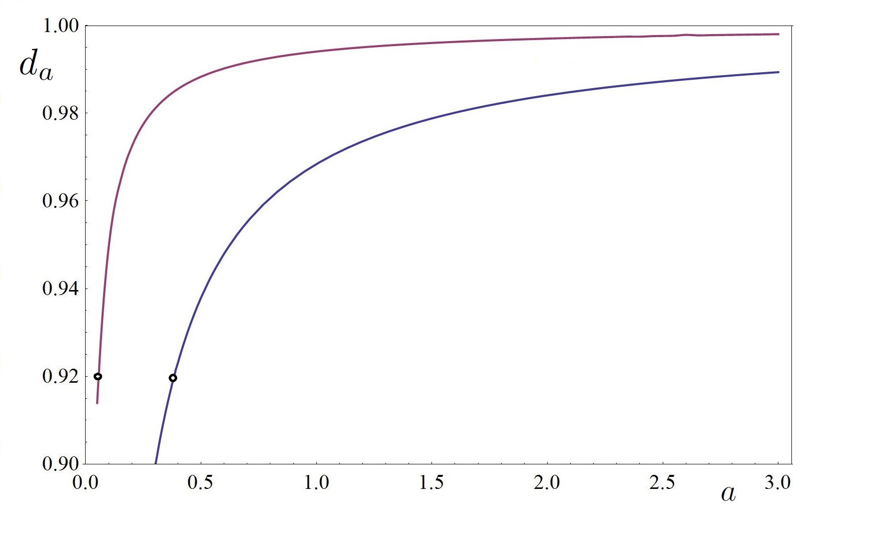
Figure 1: The lower curve shows the coefficient $d_{a}$ in Eq. (128) as a function of the RGPEP parameter $a$ in the region relevant to phenomenology. The upper curve differs from the lower one by the rough estimate of theoretical errors that is described in the text. The dots on the curves indicate the value $d_{a}=0.92$ that might correspond to a 4% change in the proton radius extracted from observed energy levels.

The lower curve results from calculating $d_{a}$ from Eq. (128). The upper curve is obtained from a similar calculation in which only the ground-state wave function $(1+p^{2})^{-2}$ is changed to $(1+p^{2})^{-2}\exp{[-4\alpha^{4}(p/a)^{4}]}$. This change is made to mimic and thus estimate the effect on wave functions of the presence of the RGPEP form factor in the effective theory with $\lambda$ given in Eq. (101). If the wave functions were calculated in a precisely derived effective theory that includes the RGPEP form factors, the wave functions would not be the same as in the ideal Schrödinger equation, Eq. (3) with a local Coulomb potential for point-like particles. Wave functions of eigenstates of a Hamiltonian including the RGPEP form factor $f$ fall off faster for large momenta than the wave functions of eigenstates of a Hamiltonian without $f$. This feature is modeled by the introduction of the exponential factor in the wave function only for orientation regarding the orders of magnitude. A rigorous estimate would require an RGPEP calculation of the effective Hamiltonian including all terms in the expansion in powers of $\alpha$ that count in comparison of theory with data with current accuracy. As mentioned more than once before, such extensive research program is far beyond the scope of this article, which merely indicates a need for carrying out such program.

V.3 Interpretation of $d_{a}$ in terms of change in proton radius

The effective Schrödinger Eq. (102) for lepton-proton bound states takes a universal scaling form of Eq. (99) when the value of the RGPEP parameter $\lambda$ is chosen differently for different leptons, see Eq. (101). This means that the standard Schrödinger picture corresponds to choosing

$$\lambda = \,a\ \sqrt{\mu\,M}\ ,$$ (129)

or

$$\lambda \sim \sqrt{\mu}\ .$$ (130)

Since the electron and muon differ in masses by the factor of about 200, the required choices of $\lambda$ differ by the factor on the order of 14.

Variation of $\lambda$ required for maintaining one and the same scaling picture of the standard Schrödinger quantum mechanics for different lepton-proton systems can be described using the parameter $a$, which changes by the factor 14 between electron-proton and muon-proton bound states. Fig. 1 shows that a change of such magnitude in $a$ can be correlated with a change in the coefficient $d_{a}$ in Eq. (122) on the order of 8%. Since the interpretation of the correction in terms of a change in the proton radius requires taking a square root of $d_{a}$, the accompanied variation in the extracted proton radius can be on the order of 4%. Since $d_{a}$ is smaller for a lighter lepton, application of the same Schrödinger equation to both types of lepton-proton bound states will produce a greater proton radius for a lighter lepton.

If one uses the same effective theory for electron-proton and muon-proton bound states, the form factor $f$ with one and the same value of $\lambda$ will fall off as a function of the relative electron-proton momentum in Hydrogen at the rate $\sqrt{m_{\mu}/m_{e}}$ times faster than as a function of the relative muon-proton momentum in a muon-proton bound state. The resulting reduction of range of the off-shellness in the interaction results in a reduction of the contribution to energy due to the proton-charge volume in the bound state and thus an increased estimate of the proton radius for a fixed value of the observed energy splitting.

VI Conclusion

The RGPEP corrections in the Schrödinger equation due to the effective nature of bound-state constituents are discussed here in the leading approximation. The corrections result solely from the form factors in the effective interactions. The form factors depend on the RGPEP scale parameter $s=1/\lambda$ and make the Coulomb potential slightly non-local at short distances. The non-locality results from the upper bound order $\lambda$ on the changes of energy (actually, invariant mass) that can be caused by the Coulomb interaction in the dynamics of effective particles.

More precisely, the upper bound on momentum changes in the RGPEP comes from an exponential function of fourth power of the ratio of momentum to the parameter $\lambda$. Since $\lambda$ needs to be on the order of masses for the effective theory to match the universal Schrödinger quantum mechanics with electromagnetic interactions, the argument of the exponential function scales as $\alpha^{4}$, on top of the Schrödinger bound-state picture which yields binding energies that scale as $\alpha^{2}$. Despite the high power of $\alpha$, the RGPEP form factor can generate a noticeable correction in the extracted proton radius because it affects the lepton-proton relative-motion wave function at the origin.

The conceptual import of the RGPEP is that the bound-state constituents in the non-relativistic Schrödinger quantum mechanics are not point-like and they interact at short distances by a potential that slightly differs from the Coulomb potential for point-like charges. The effective nature of constituents can be studied using the RGPEP in QFT.

Although the reasoning offered in this article is focused on a specific term in the lepton-proton bound-state dynamics, the RGPEP used in this reasoning offers also access to corrections due to effective nature of particles in all areas of physics where equations of the Schrödinger type apply. This means that in all such cases one is obliged to determine the scale of energy changes that an effective interaction can cause and the presence of such scale must be taken into account in interpretation of precise comparisons between theory and experiment.

Acknowledgment

It is a pleasure to thank Krzysztof Pachucki for his comments on the author’s ideas presented here.

Appendix A Canonical Hamiltonian

The local action to consider is

$$S = \int d^{4}x\,{\cal L}\,=\,{1\over 2}\int dx^{+}dx^{-}d^{2}x^{\perp}\,{\cal L}\,,$$ (131)

where

$${\cal L} = -{1\over 4}F_{\mu\nu}F^{\mu\nu}+\sum_{n=1}^{3}\bar{\psi}_{n}(i\partial/-e_{n}A/-m_{n})\psi\ ,$$ (132)

and subscripts $n=1,2,3$ refer to electrons, muons and protons, respectively. At this point, proton is considered point-like and essentially of the same properties as leptons except for opposite charge and different mass. The corresponding canonical FF Hamiltonian in the gauge $A^{+}=0$ is yan4

$$P^{-} = {1\over 2}\int dx^{-}d^{2}x^{\perp}\,T^{+\,-}\ .$$ (133)

We use the same convention for components of all tensors as in the case of Minkowski’s space-time coordinates, for which

$$x^{\pm} = x^{0}\pm x^{3}\,,$$ (134)

$$x^{\perp} = (x^{1},x^{2})\,.$$ (135)

The co-ordinate $x^{+}$ plays the role of evolution parameter, or FF “time,” and $x^{\perp}$ and $x^{-}$ play the roles of space co-ordinates in the front hyperplane in space-time.

The energy-momentum tensor density component $T^{+\,-}$ is

$$T^{+\,-} = A^{\perp}\,(i\partial^{\perp})^{2}A^{\perp}+\sum_{n=1}^{3}\psi_{n+}^{\dagger}\left[(i\partial^{\perp}\alpha^{\perp}+\beta m_{n})-e_{n}A^{\perp}\alpha^{\perp}\right]\,{2\over i\partial^{+}}\,\left[(i\partial^{\perp}\alpha^{\perp}+\beta m_{n})-e_{n}A^{\perp}\alpha^{\perp}\right]\,\psi_{n+}$$ (136)

$$+ \sum_{n=1}^{3}2e_{n}\psi_{n+}^{\dagger}\psi_{+n}\,{2\over i\partial^{+}}\,i\partial^{\perp}A^{\perp}+\sum_{n,l=1}^{3}2e_{n}\psi_{n+}^{\dagger}\psi_{n+}\,{1\over(i\partial^{+})^{2}}\,2e_{l}\psi_{l+}^{\dagger}\psi_{l+}\ ,$$

and for all fermion fields equally $\psi_{\pm}=\Lambda_{\pm}\psi$ and $\Lambda_{\pm}=\gamma^{0}\gamma^{+}/2$. The Hamiltonian can be written as

$$P^{-} = \int dx^{-}d^{2}x^{\perp}\,\left\{{1\over 2}A_{\mu}\,\partial^{\perp\,2}A^{\mu}+\sum_{n=1}^{3}\left[\bar{\psi}_{n}\gamma^{+}{-\partial^{\perp\,2}+m_{n}^{2}\over 2i\partial^{+}}\,\psi_{n}\right.\right.$$

$$+ \left.\left.e_{n}\,\bar{\psi}_{n}A/\,\psi_{n}+e_{n}^{2}\,\bar{\psi}_{n}A/\,{\gamma^{+}\over 2i\partial^{+}}\,A/\,\psi_{n}+e_{n}\bar{\psi}_{n}\gamma^{+}\psi_{n}\,{1\over 2(i\partial^{+})^{2}}\,\sum_{k=1}^{3}\,e_{k}\,\bar{\psi}_{k}\gamma^{+}\psi_{k}\right]\right\}\,,$$

where the dependent components of fields, $A^{-}$ and $\psi_{n-}$, are solutions to the constraint equations with all the electric charges $e_{n}$ set to zero. It is visible that the Hamiltonian density contains terms bilinear, trilinear and quadrilinear in the fields. Namely,

$$P^{-}_{2} = \int dx^{-}d^{2}x^{\perp}\,{1\over 2}A_{\mu}\,\partial^{\perp\,2}A^{\mu}+\int dx^{-}d^{2}x^{\perp}\,\sum_{n=1}^{3}\bar{\psi}_{n}\gamma^{+}{-\partial^{\perp\,2}+m_{n}^{2}\over 2i\partial^{+}}\,\psi_{n}\,,$$ (138)

$$P^{-}_{3} = \int dx^{-}d^{2}x^{\perp}\,\sum_{n=1}^{3}\,e_{n}\,\bar{\psi}_{n}A/\,\psi_{n}\,,$$ (139)

$$P^{-}_{4} = \int dx^{-}d^{2}x^{\perp}\,\sum_{n=1}^{3}\left[e_{n}^{2}\,\bar{\psi}_{n}A/\,{\gamma^{+}\over 2i\partial^{+}}\,A/\,\psi_{n}+e_{n}\bar{\psi}_{n}\gamma^{+}\psi_{n}\,{1\over 2(i\partial^{+})^{2}}\,\sum_{k=1}^{3}\,e_{k}\,\bar{\psi}_{k}\gamma^{+}\psi_{k}\right]\,.$$ (140)

A.1 Quantization

The quantum Hamiltonian is obtained by replacing fields $A^{\perp}$ and $\psi_{n+}$ by field operators $\hat{A}^{\perp}$ and $\hat{\psi}_{n+}$, regulating the inverse powers of $i\partial^{+}$ in the same way the field operators are regulated, and normal ordering. Using the creation and annihilation operators that are assumed to satisfy the commutation relations

$$\left\{b_{nps},b^{\dagger}_{n^{\prime}p^{\prime}s^{\prime}}\right\} = \left\{d_{nps},d^{\dagger}_{n^{\prime}p^{\prime}s^{\prime}}\right\}\,=\,2p^{+}(2\pi)^{3}\delta^{3}(p-p^{\prime})\,\delta_{ss^{\prime}}\,\delta_{nn^{\prime}}\,,$$ (141)

$$\left[a_{ps},a^{\dagger}_{p^{\prime}s^{\prime}}\right] = 2p^{+}(2\pi)^{3}\delta^{3}(p-p^{\prime})\,\delta_{ss^{\prime}}\,,$$ (142)

with other relations being zero, respectively, the field operators are written as (for our conventions concerning notation for fermions, see fermions )

$$\hat{\psi}_{n+}(x) = \sum_{s}\int_{p}\ \Delta^{1/2}(p)\,\sqrt{p^{+}}\,\left[b_{nps}-d_{nps}^{\dagger}\,\sigma^{1}\right]\,\left[\begin{array}[]{c}\chi_{s}\\ 0\end{array}\right]\,e^{-ic_{p}p\,x-\epsilon|x|}\,,$$ (145)

$$\hat{A}^{\perp}(x) = \sum_{s}\int_{p}\ \Delta^{1/2}(p)\left[a_{ps}\,\varepsilon_{s}^{\perp}+a_{ps}^{\dagger}\,\varepsilon_{s}^{\perp*}\right]\,e^{-ic_{p}p\,x-\epsilon|x|}\,,$$ (146)

where

$$\int_{p} = \int{dp^{+}\ d^{2}p^{\perp}\over 2p^{+}(2\pi)^{3}}\ \theta(p^{+})\ ,$$ (147)

and $\Delta(p)$ denotes the regularization function,

$$\Delta(p)\ = \Delta\left(|p^{+}|,|p^{\perp}|\right)\,.$$ (148)

This function is required to tend to zero when momentum $|p^{\perp}|$ tends to infinity or $|p^{+}|$ tends to zero, because divergences occur due to large $|p^{\perp}|$ and small $|p^{+}|$. Hence, the regularization requires two parameters. For example, if one used the regulator function of the form Glazek1994

$$\Delta(p) = \exp\left(-\,{|p^{\perp}|^{2}+\delta^{2}\over|p^{+}|\,\Delta}\right)\,,$$ (149)

the parameter $\Delta$ would limit $|p^{\perp}|$ from above and $\delta^{2}/\Delta$ would limit $|p^{+}|$ from below. In the no-cutoff limit, $\Delta$ tends to infinity and $\delta$ tends to zero. Other functions $\Delta(p)$ can be considered, especially such that factorize into the transverse and longitudinal regulating functions. The same function $\Delta$ is applied in regularization of the constraint equations. This regularization introduces factors $\Delta(p)$ in quadrilinear terms with $1/p^{+}$ and $1/p^{+\,2}$.

The smooth exponential damping factors $e^{-\epsilon|x|}$ are introduced to eliminate boundary effects in a large quantization box in “space” directions of $x^{\perp}$ and $x^{-}$. This means that one only focuses on the phenomena that fit well within the box of size $L\gg\epsilon^{-1}$. The principles of building the box are the same as in the formal scattering theory GellMannGoldberger .

Spinors $\chi_{s}$ stand for the standard Pauli two component spinors and the photon polarization vectors are defined by writing $\varepsilon_{s}^{\perp}=(1,is)/\sqrt{2}$ with $s=\pm 1$ and the operators corresponding to $s=+1$ ($s=-1$) often labeled as 1(2) or $+$($-$).

The coefficients $c_{p}$ in the Fourier-transform exponentials are introduced for handling creation and annihilation operators in a generic operator calculus. We define $c_{p}$ by the rule that $c_{p}=1$ in a formula containing an annihilation operator with quantum numbers denoted by $p$, and $c_{p}=-1$ in a formula containing a creation operator with these quantum numbers. The generic factor of momentum conservation in interaction terms is denoted by

$$\tilde{\delta} = 2(2\pi)^{3}\delta^{3}\left(\sum_{l}c_{p_{l}}p_{l}\right)\,,$$ (150)

where $l$ runs from 1 to the number of fields in a term.

The quantum canonical Hamiltonian is a sum of terms that are bilinear, trilinear and quadrilinear in creation and annihilation operators. Namely,

$$\hat{P}^{-} = \hat{P}^{-}_{2}+\hat{P}^{-}_{3}+\hat{P}^{-}_{4}\,,$$ (151)

where each term corresponds to its classical counterpart in Eqs. (138) to (140). Explicit expressions for all terms in $\hat{P}^{-}$ are listed below in separate subsections.

A.2 Bilinear terms

The bilinear terms are

$$\hat{P}^{-}_{2} = \sum_{s}\int_{p}\Delta(p)\ \left[{p^{\perp\,2}\over p^{+}}\,a_{ps}^{\dagger}a_{ps}+\sum_{n=1}^{3}{p^{\perp\,2}+m_{n}^{2}\over p^{+}}\,\left(b_{ps}^{\dagger}b_{ps}+d_{ps}^{\dagger}d_{ps}\right)\right]+C_{A}+C_{\psi}\,,$$ (152)

where

$$C_{A} = {1\over 2}\sum_{s}\int_{p}\ \Delta(p)\ 2p^{+}(2\pi)^{3}\delta^{3}(0)\,{p^{\perp\,2}\over p^{+}}\,,$$ (153)

$$C_{\psi} = -\sum_{s}\int_{p}\ \Delta(p)\ 2p^{+}(2\pi)^{3}\delta^{3}(0)\,\sum_{n=1}^{3}{p^{\perp\,2}+m_{n}^{2}\over p^{+}}\ .$$ (154)

The constants $C_{A}$ and $C_{\psi}$ result from commuting operators during normal ordering. As additive constants in the Hamiltonian, they could be ignored in quantum mechanics. However, one could include them in variational FF estimates of the vacuum energy if one wanted to recreate the vacuum effects known to cause problems in the IF of quantum field theory in $3+1$ dimensions BartnikGlazek . Here, they are removed from the calculation.

A.3 Trilinear terms

The trilinear terms are

$$\hat{P}_{3}^{-} = \sum_{n=1}^{3}\hat{P}_{3n}\,,$$ (155)

where

$$\hat{P}_{3n} = -e_{n}\sum_{s_{1}s_{2}}\int_{p_{1}p_{2}q}\sqrt{\Delta(p_{1})\Delta(p_{2})\Delta(q)}\ \tilde{\delta}\ \sqrt{2p_{1}^{+}p_{2}^{+}}\ \hat{Y}_{n}\,,$$ (156)

and $\hat{Y}_{n}$ involves only operators and masses for fermions number $n$, according to the same pattern. Namely,

$$\hat{Y} = b^{\dagger}_{p_{1}s_{1}}b_{p_{2}s_{2}}\,a_{q+}\,\left[\left({p_{2}\over p_{2}^{+}}-{q\over q^{+}}\right)\,\delta_{s_{1}1}\delta_{s_{2}1}+\left({p_{1}\over p_{1}^{+}}-{q\over q^{+}}\right)\,\delta_{s_{2}-1}\delta_{s_{1}-1}+\left({m\over p_{2}^{+}}-{m\over p_{1}^{+}}\right)\delta_{s_{1}1}\delta_{s_{2}-1}\right]$$ (157)

$$+ b^{\dagger}_{p_{1}s_{1}}b_{p_{2}s_{2}}\,a_{q-}^{\dagger}\,\left[\left({p_{2}\over p_{2}^{+}}-{q\over q^{+}}\right)\,\delta_{s_{1}1}\delta_{s_{2}1}+\left({p_{1}\over p_{1}^{+}}-{q\over q^{+}}\right)\,\delta_{s_{2}-1}\delta_{s_{1}-1}+\left({m\over p_{2}^{+}}-{m\over p_{1}^{+}}\right)\delta_{s_{1}1}\delta_{s_{2}-1}\right]$$

$$+ b^{\dagger}_{p_{1}s_{1}}b_{p_{2}s_{2}}\,a_{q-}\,\left[\left({p_{2}^{*}\over p_{2}^{+}}-{q^{*}\over q^{+}}\right)\,\delta_{s_{1}-1}\delta_{s_{2}-1}+\left({p_{1}^{*}\over p_{1}^{+}}-{q^{*}\over q^{+}}\right)\,\delta_{s_{2}1}\delta_{s_{1}1}+\left({m\over p_{1}^{+}}-{m\over p_{2}^{+}}\right)\,\delta_{s_{2}1}\delta_{s_{1}-1}\right]$$

$$+ b^{\dagger}_{p_{1}s_{1}}b_{p_{2}s_{2}}\,a_{q+}^{\dagger}\,\left[\left({p_{2}^{*}\over p_{2}^{+}}-{q^{*}\over q^{+}}\right)\,\delta_{s_{1}-1}\delta_{s_{2}-1}+\left({p_{1}^{*}\over p_{1}^{+}}-{q^{*}\over q^{+}}\right)\,\delta_{s_{2}1}\delta_{s_{1}1}+\left({m\over p_{1}^{+}}-{m\over p_{2}^{+}}\right)\,\delta_{s_{2}1}\delta_{s_{1}-1}\right]$$

$$+ b^{\dagger}_{p_{1}s_{1}}d_{p_{2}s_{2}}^{\dagger}\,a_{q+}\,\left[-\left({p_{2}\over p_{2}^{+}}-{q\over q^{+}}\right)\,\delta_{s_{1}1}\delta_{s_{2}-1}-\left({p_{1}\over p_{1}^{+}}-{q\over q^{+}}\right)\,\delta_{s_{2}1}\delta_{s_{1}-1}+\left({m\,\over p_{2}^{+}}+{m\over p_{1}^{+}}\right)\,\,\delta_{s_{2}1}\delta_{s_{1}1}\right]$$

$$+ b^{\dagger}_{p_{1}s_{1}}d_{p_{2}s_{2}}^{\dagger}\,a_{q-}\,\left[-\left({p^{*}_{2}\over p_{2}^{+}}-{q^{*}\over q^{+}}\right)\,\delta_{s_{1}-1}\delta_{s_{2}1}-\left({p_{1}^{*}\over p_{1}^{+}}-{q^{*}\over q^{+}}\right)\,\delta_{s_{2}-1}\delta_{s_{1}1}-\left({m\,\over p_{2}^{+}}+{m\over p_{1}^{+}}\right)\,\,\delta_{s_{2}-1}\delta_{s_{1}-1}\right]$$

$$+ d_{p_{1}s_{1}}b_{p_{2}s_{2}}\,a_{q+}^{\dagger}\,\left[-\left({p^{*}_{2}\over p_{2}^{+}}-{q^{*}\over q^{+}}\right)\,\delta_{s_{1}1}\delta_{s_{2}-1}-\left({p_{1}^{*}\over p_{1}^{+}}-{q^{*}\over q^{+}}\right)\,\delta_{s_{2}1}\delta_{s_{1}-1}+\left({m\,\over p_{2}^{+}}+{m\over p_{1}^{+}}\right)\,\,\delta_{s_{2}1}\delta_{s_{1}1}\right]$$

$$+ d_{p_{1}s_{1}}b_{p_{2}s_{2}}\,a_{q-}^{\dagger}\,\left[-\left({p_{2}\over p_{2}^{+}}-{q\over q^{+}}\right)\,\delta_{s_{1}-1}\delta_{s_{2}1}-\left({p_{1}\over p_{1}^{+}}-{q\over q^{+}}\right)\,\delta_{s_{2}-1}\delta_{s_{1}1}-\left({m\,\over p_{2}^{+}}+{m\over p_{1}^{+}}\right)\,\,\delta_{s_{2}-1}\delta_{s_{1}-1}\right]$$

$$- d_{p_{2}s_{2}}^{\dagger}d_{p_{1}s_{1}}\,a_{q+}\,\left[\left({p_{2}\over p_{2}^{+}}-{q\over q^{+}}\right)\,\delta_{s_{1}-1}\delta_{s_{2}-1}+\left({p_{1}\over p_{1}^{+}}-{q\over q^{+}}\right)\,\delta_{s_{2}1}\delta_{s_{1}1}+\left({m\over p_{1}^{+}}-{m\over p_{2}^{+}}\right)\,\delta_{s_{2}1}\delta_{s_{1}-1}\right]$$

$$- d_{p_{2}s_{2}}^{\dagger}d_{p_{1}s_{1}}\,a_{q-}^{\dagger}\,\left[\left({p_{2}\over p_{2}^{+}}-{q\over q^{+}}\right)\,\delta_{s_{1}-1}\delta_{s_{2}-1}+\left({p_{1}\over p_{1}^{+}}-{q\over q^{+}}\right)\,\delta_{s_{2}1}\delta_{s_{1}1}+\left({m\over p_{1}^{+}}-{m\over p_{2}^{+}}\right)\,\delta_{s_{2}1}\delta_{s_{1}-1}\right]$$

$$- d_{p_{2}s_{2}}^{\dagger}d_{p_{1}s_{1}}\,a_{q-}\,\left[\left({p_{2}^{*}\over p_{2}^{+}}-{q^{*}\over q^{+}}\right)\,\delta_{s_{1}1}\delta_{s_{2}1}+\left({p_{1}^{*}\over p_{1}^{+}}-{q^{*}\over q^{+}}\right)\,\delta_{s_{2}-1}\delta_{s_{1}-1}+\left({m\over p_{2}^{+}}-{m\over p_{1}^{+}}\right)\delta_{s_{1}1}\delta_{s_{2}-1}\right]$$

$$- d_{p_{2}s_{2}}^{\dagger}d_{p_{1}s_{1}}\,a_{q+}^{\dagger}\,\left[\left({p_{2}^{*}\over p_{2}^{+}}-{q^{*}\over q^{+}}\right)\,\delta_{s_{1}1}\delta_{s_{2}1}+\left({p_{1}^{*}\over p_{1}^{+}}-{q^{*}\over q^{+}}\right)\,\delta_{s_{2}-1}\delta_{s_{1}-1}+\left({m\over p_{2}^{+}}-{m\over p_{1}^{+}}\right)\delta_{s_{1}1}\delta_{s_{2}-1}\right]\,,$$

where the subscript $n$ is omitted. The momentum variables $p_{1}$, $p_{2}$ and $q$ are complex numbers defined according to the rule

$$p = p^{1}+ip^{2}\ .$$ (158)

There are no terms resulting from commuting operators during normal ordering because of the momentum conservation and presence of regularization factor $\Delta$ in the Fourier expansion of fields.

A.4 Quadrilinear terms

There are two kinds of quadrilinear terms. One involves fermions and photons, denoted by $\hat{P}^{-}_{4\psi A}$, and the other one, analogous to the instantaneous Coulomb potential in the IF of dynamics, involves only fermions and is denoted by $\hat{P}^{-}_{4\psi\psi}$. These terms are described in two separate subsections.

A.4.1 Quadrilinear fermion-photon couplings $\hat{P}^{-}_{4\psi A}$

The quadrilinear term $\hat{P}_{4\psi A}$ is a sum of terms for three kinds of fermions,

$$\hat{P}_{4\psi A}^{-} = \sum_{n=1}^{3}\hat{P}_{4\psi_{n}A}^{-}\ ,$$ (159)

where

$$\hat{P}_{4\psi_{n}A}^{-} = e_{n}^{2}\sum_{s_{1}s_{2}r_{1}r_{2}}\int_{p_{1}p_{2}q_{1}q_{2}}\ \sqrt{\Delta(p_{1})\Delta(p_{2})\Delta(q_{1})\Delta(q_{2})}\ \tilde{\delta}\,\sqrt{p_{1}^{+}p_{2}^{+}}\ \,{2\Delta(c_{q_{2}}q_{2}+c_{p_{2}}p_{2})\over c_{q_{2}}q_{2}^{+}+c_{p_{2}}p_{2}^{+}}\ \hat{Z}_{n}$$ (160)

$$+ \sum_{r}\int_{q}\Delta(q)\ {\delta m_{n\gamma}^{2}\over q^{+}}\ a_{qr}^{\dagger}a_{qr}+\sum_{s}\int_{p}\Delta(p)\ \left[{\delta m_{n}^{2}\over p^{+}}\ b_{nps}^{\dagger}b_{nps}+{\delta m_{\bar{n}}^{2}\over p^{+}}\ d_{nps}^{\dagger}d_{nps}\right]+C_{\psi_{n}A}\ .$$

Omitting the subscript $n$ in subscripts of creation and annihilation operators for fermions,

$$\hat{Z}_{n} = \left[\delta_{s_{1}\,c_{q_{1}}r_{1}}\delta_{s_{2}\,c_{q_{1}}r_{1}}\ b_{p_{1}s_{1}}^{\dagger}b_{p_{2}s_{2}}-\delta_{s_{1}\,c_{q_{1}}r_{1}}\delta_{s_{2}\,c_{q_{2}}r_{2}}\ b_{p_{1}s_{1}}^{\dagger}d_{p_{2}s_{2}}^{\dagger}\right.$$ (161)

$$- \left.\delta_{s_{1}\,c_{q_{2}}r_{2}}\delta_{s_{2}\,c_{q_{1}}r_{1}}\ d_{p_{1}s_{1}}b_{p_{2}s_{2}}-\delta_{s_{1}\,c_{q_{2}}r_{2}}\delta_{s_{2}\,c_{q_{2}}r_{2}}\ d_{p_{2}s_{2}}^{\dagger}d_{p_{1}s_{1}}\right]$$

$$\times \left[a_{q_{1}r_{1}}a_{q_{2}r_{2}}+a_{q_{2}r_{2}}^{\dagger}a_{q_{1}r_{1}}+a_{q_{1}r_{1}}^{\dagger}a_{q_{2}r_{2}}+a_{q_{1}r_{1}}^{\dagger}a_{q_{2}r_{2}}^{\dagger}\right]\ \delta_{c_{q_{1}}r_{1}\,-c_{q_{2}}r_{2}}\ .$$

The terms with only creation or only annihilation operators do not actually contribute because of the conservation of $p^{+}$ and presence of the regularization factors. Normal ordering proceeds through commuting operators and thus producing the mass-like terms

$$\delta m_{n\gamma}^{2} = 2e_{n}^{2}\int_{p}\ p^{+}\ \Delta(p)\ \left[{\Delta(q-p)\over q^{+}-p^{+}}-{\Delta(q+p)\over q^{+}+p^{+}}\right]\ ,$$ (162)

$$\delta m_{n}^{2} = 2e_{n}^{2}\int_{q}\ p^{+}\ \Delta(q)\ {\Delta(p-q)\over p^{+}-q^{+}}\ ,$$ (163)

$$\delta m_{\bar{n}}^{2} = 2e_{n}^{2}\int_{q}\ p^{+}\ \Delta(q)\ {\Delta(p+q)\over p^{+}+q^{+}}\ ,$$ (164)

and a number

$$C_{\psi_{n}A} = -2(2\pi)^{3}\delta^{3}(0)\ 4e_{n}^{2}\int_{pq}\ \Delta(p)\Delta(q)\ p^{+}\ {\Delta(p+q)\over p^{+}+q^{+}}\ .$$ (165)

All these terms are removed. They depend on the regularization function $\Delta(p)$ and ought to be subtracted anyway. In the case of $\Delta(p)$ in Eq. (149) that correlates $\perp$ and $+$ components of momentum, one may have to consider constants and operators of the type $e^{2}\Delta A^{\perp}i\partial^{+}A^{\perp}$ or $e^{2}\Delta\bar{\psi}\gamma^{+}\psi$ that do not obey regular FF power counting Wilsonetal .

Regarding protons, one should remember that they are not physically point-like in the sense that leptons are. The canonical terms in a local theory for protons is merely a method of book-keeping that applies only for the momentum transfers smaller than the inverse of their size.

A.4.2 Quadrilinear fermion couplings $\hat{P}_{4\psi\psi}^{-}$

The fermion quadrilinear term $\hat{P}^{-}_{4\psi\psi}$ is the FF analog of the IF Coulomb term. It has the form

$$\hat{P}^{-}_{4\psi\psi} = \sum_{n=1}^{3}\hat{P}^{-}_{4\psi_{n}\psi}\,,$$ (166)

where

$$\hat{P}^{-}_{4\psi_{n}\psi} = e_{n}\sum_{l=1}^{3}e_{l}\sum_{s_{1}s_{2}s_{3}s_{4}}\int_{p_{1}p_{2}p_{3}p_{4}}\,\sqrt{\Delta(p_{1})\Delta(p_{2})\Delta(p_{3})\Delta(p_{4})}\ \tilde{\delta}\ \sqrt{p_{1}^{+}p_{2}^{+}p_{3}^{+}p_{4}^{+}}\ {2\Delta(c_{3}p_{3}+c_{4}p_{4})\over(c_{3}p_{3}^{+}+c_{4}p_{4}^{+})^{2}}\ \hat{X}_{nl}\ .$$ (167)

Using momentum conservation, properties of the regularization factors, and performing normal ordering, one can write the terms that contribute to $\hat{X}_{nl}$ in the form

$$\hat{X}_{nl} = \hat{X}_{4nl}+\hat{X}_{2nl}+X_{0nl}\ .$$ (168)

Genuine four-fermion interactions result from

$$\hat{X}_{4nl} = -\delta_{s_{1}s_{2}}\delta_{s_{3}s_{4}}\ b_{np_{1}s_{1}}^{\dagger}b_{lp_{3}s_{3}}^{\dagger}b_{np_{2}s_{2}}b_{lp_{4}s_{4}}$$ (169)

$$- \delta_{s_{1}s_{2}}\delta_{s_{3}-s_{4}}\ b_{np_{1}s_{1}}^{\dagger}b_{lp_{3}s_{3}}^{\dagger}d_{lp_{4}s_{4}}^{\dagger}b_{lnp_{2}s_{2}}$$

$$- \delta_{s_{1}s_{2}}\delta_{s_{3}-s_{4}}\ b_{np_{1}s_{1}}^{\dagger}b_{np_{2}s_{2}}d_{lp_{3}s_{3}}b_{lp_{4}s_{4}}$$

$$+ \delta_{s_{1}s_{2}}\delta_{s_{3}s_{4}}\ b_{np_{1}s_{1}}^{\dagger}d_{lp_{4}s_{4}}^{\dagger}b_{np_{2}s_{2}}d_{lp_{3}s_{3}}$$

$$- \delta_{s_{1}-s_{2}}\delta_{s_{3}s_{4}}\ b_{np_{1}s_{1}}^{\dagger}d_{np_{2}s_{2}}^{\dagger}b_{lp_{3}s_{3}}^{\dagger}b_{lp_{4}s_{4}}$$

$$+ \delta_{s_{1}-s_{2}}\delta_{s_{3}-s_{4}}\ b_{np_{1}s_{1}}^{\dagger}d_{np_{2}s_{2}}^{\dagger}d_{lp_{3}s_{3}}b_{lp_{4}s_{4}}$$

$$+ \delta_{s_{1}-s_{2}}\delta_{s_{3}s_{4}}\ b_{np_{1}s_{1}}^{\dagger}d_{np_{2}s_{2}}^{\dagger}d_{lp_{4}s_{4}}^{\dagger}d_{lp_{3}s_{3}}$$

$$- \delta_{s_{1}-s_{2}}\delta_{s_{3}s_{4}}\ b_{lp_{3}s_{3}}^{\dagger}d_{np_{1}s_{1}}b_{np_{2}s_{2}}b_{lp_{4}s_{4}}$$

$$- \delta_{s_{1}-s_{2}}\delta_{s_{3}-s_{4}}\ b_{lp_{3}s_{3}}^{\dagger}d_{lp_{4}s_{4}}^{\dagger}b_{np_{2}s_{2}}d_{np_{1}s_{1}}$$

$$+ \delta_{s_{1}-s_{2}}\delta_{s_{3}s_{4}}\ d_{lp_{4}s_{4}}^{\dagger}d_{np_{1}s_{1}}b_{np_{2}s_{2}}d_{lp_{3}s_{3}}$$

$$+ \delta_{s_{1}s_{2}}\delta_{s_{3}s_{4}}\ d_{np_{2}s_{2}}^{\dagger}b_{lp_{3}s_{3}}^{\dagger}d_{np_{1}s_{1}}b_{lp_{4}s_{4}}$$

$$+ \delta_{s_{1}s_{2}}\delta_{s_{3}-s_{4}}\ d_{np_{2}s_{2}}^{\dagger}b_{lp_{3}s_{3}}^{\dagger}d_{lp_{4}s_{4}}^{\dagger}d_{np_{1}s_{1}}$$

$$+ \delta_{s_{1}s_{2}}\delta_{s_{3}-s_{4}}\ d_{np_{2}s_{2}}^{\dagger}d_{np_{1}s_{1}}d_{lp_{3}s_{3}}b_{lp_{4}s_{4}}$$

$$- \delta_{s_{1}s_{2}}\delta_{s_{3}s_{4}}\ d_{np_{2}s_{2}}^{\dagger}d_{lp_{4}s_{4}}^{\dagger}d_{np_{1}s_{1}}d_{lp_{3}s_{3}}\ .$$

The mass-like terms in $\hat{P}_{4\psi\psi}^{-}$ that result from commuting operators during normal ordering are due to $\hat{X}_{2nl}$. Namely,

$$\hat{P}^{-}_{4\psi\psi\,mass} = \sum_{s}\int_{p}\Delta(p)\ {\delta m_{\psi\psi}^{2}\over p^{+}}\ \left(b_{ps}^{\dagger}b_{ps}+d_{ps}^{\dagger}d_{ps}\right)\ ,$$ (170)

where

$$\delta m_{\psi\psi}^{2} = 2e^{2}\int_{q}\ p^{+}q^{+}\ \Delta(q)\ \left[{\Delta(p-q)\over(p^{+}-q^{+})^{2}}-{\Delta(p+q)\over(p^{+}+q^{+})^{2}}\right]\,.$$ (171)

Again, these depend on the regularization function $\Delta$ and are removed. In the case of Eq. (149) one would have to consider similar terms as in $\hat{P}^{-}_{4\psi A}$ but with additional logarithms of $|\Delta i\partial^{+}|/\delta^{2}$.

The additive constant that one obtains in the canonical Hamiltonian by integrating

$$X_{0nl} = \delta_{nl}\ \left[\delta_{s_{1}-s_{2}}\delta_{s_{3}-s_{4}}\ \delta_{23}\ \delta_{14}+\delta_{s_{1}s_{2}}\delta_{s_{3}s_{4}}\ \delta_{12}\ \delta_{34}\right]\ ,$$ (172)

can be ignored without any consequence in the lepton-proton bound-state equation.

Appendix B Outline of the RGPEP

The coefficients of powers of $q_{t}$ in ${\cal H}_{t}(q_{t})$ are found in the RGPEP using Eq. (14) and calculating ${\cal H}_{t}(q_{0})$. Differentiation of

$${\cal H}_{t}(q_{0}) = {\cal U}^{\dagger}_{t}\,{\cal H}_{0}(q_{0})\,{\cal U}_{t}\,,$$ (173)

with respect to $t$ yields

$${\cal H}^{\prime}_{t}(q_{0}) = [{\cal G}_{t}(q_{0}),{\cal H}_{t}(q_{0})]$$ (174)

with the generator ${\cal G}_{t}=-{\cal U}_{t}^{\dagger}{\cal U}^{\prime}_{t}$ and

$${\cal U}_{t} = T\exp{\left(-\int_{0}^{t}d\tau\,{\cal G}_{\tau}\right)}\,.$$ (175)

$T$ denotes ordering in $\tau$. We consider the generator Glazek1998 ; QQ

$${\cal G}_{t} = \left\{(1-f^{-1}){\cal H}_{t}\right\}_{{\cal H}_{f}}$$ (176)

and pRGPEP

$${\cal G}_{t} = [{\cal H}_{f},{\cal H}_{Pt}]\,.$$ (177)

The operator ${\cal H}_{f}$, called the free Hamiltonian, is the part of ${\cal H}_{0}(q_{0})$ that does not depend on the coupling constants,

$${\cal H}_{f} = \sum_{i}\,p_{i}^{-}\,q^{\dagger}_{0i}q_{0i}\,,$$ (178)

where $i$ denotes particle species and $p_{i}^{-}$ is the free FF energy of a particle with mass $m_{i}$ and kinematical momentum components $p_{i}^{+}$ and $p_{i}^{\perp}$,

$$p^{-}_{i} = {p_{i}^{\perp\,2}+m_{i}^{2}\over p_{i}^{+}}\,.$$ (179)

The curly bracket with subscript ${\cal H}_{f}$ in Eq. (176) means that by definition ${\cal G}_{t}$ satisfies the equation $\left[{\cal G}_{t},{\cal H}_{f}\right]=(1-f^{-1}){\cal H}_{t}$. The form factor $f$ depends on the difference between free invariant masses of the right (R) and left (L) sets of particles that are involved in interaction in a Hamiltonian matrix element. Thus, R and L refer to the effective particles that enter and emerge from the interaction. The form factor is

$$f = e^{-t({\cal M}_{L}^{2}-{\cal M}^{2}_{R})^{2}}\,.$$ (180)

The operator ${\cal H}_{Pt}$ is defined for any polynomial ${\cal H}_{t}$,

$${\cal H}_{t}(q_{0})=\sum_{n=2}^{\infty}\,\sum_{i_{1},i_{2},...,i_{n}}\,c_{t}(i_{1},...,i_{n})\,\,q^{\dagger}_{0i_{1}}\cdot\cdot\cdot q_{0i_{n}}\,,$$ (181)

by multiplication of each and every term in it by a square of a total $+$ momentum involved in a term,

$${\cal H}_{Pt}(q_{0}) = \sum_{n=2}^{\infty}\,\sum_{i_{1},i_{2},...,i_{n}}\,c_{t}(i_{1},...,i_{n})\,\left({1\over 2}\sum_{k=1}^{n}p_{i_{k}}^{+}\right)^{2}\,\,q^{\dagger}_{0i_{1}}\cdot\cdot\cdot q_{0i_{n}}\,.$$ (182)

The multiplication secures that Hamiltonians ${\cal H}_{t}$ possess 7 kinematical symmetries of the FF dynamics. The factor 1/2 is needed because the sum includes both incoming and outgoing particles that have the same total momentum.

Solutions to the RGPEP equation can be expanded in powers of the charge $e$,

$${\cal H}_{t} = {\cal H}_{f}+e{\cal H}_{t}^{(1)}+e^{2}{\cal H}_{t}^{(2)}+...\ .$$ (183)

Up to order $e^{2}$ the bare charge and the renormalized charge are the same and the terms of formal order $e$ and $e^{2}$ in the effective Hamiltonian read

$${\cal H}_{t\,ab}^{(1)} = f_{ab}\,{\cal H}_{0\,ab}^{(1)}\,,$$ (184)

$${\cal H}_{t\,ab}^{(2)} = f_{ab}\left[{\cal H}_{0\,ab}^{(2)}+\sum_{x}{\cal F}_{axb}{\cal H}_{0\,ax}^{(1)}{\cal H}_{0\,xb}^{(1)}\right]\,,$$ (185)

where, according to Eq. (180) with $L=a$ and $R=b$, $f_{ab}=\exp{(-t\,ab^{2})}$. In case of the generator given in Eq. (176),

$${\cal F}_{axb} = {p_{ax}\,ax+p_{bx}\,bx\over ax^{2}+xb^{2}}\,\left[1-e^{-t(ax^{2}+xb^{2})}\right]\,.$$ (186)

In case of the generator given in Eq. (177),

$${\cal F}_{axb} = {p_{ax}\,ax+p_{bx}\,bx\over ax^{2}+xb^{2}-ab^{2}}\,\left[1-e^{-t(ax^{2}+xb^{2}-ab^{2})}\right]\,.$$ (187)

Both cases will lead to the same conclusion concerning the proton radius in lepton-proton bound states. Extensive explanation of the symbols used in the above formulas can be found in pRGPEP . Symbols $a$, $b$ and $x$ denote the left, intermediate and right configurations of the effective particles that participate in the interaction, respectively. Symbols such as $p_{ax}$ denote the total $p^{+}$ of particles involved in the interaction, which is sandwiched between states corresponding in this case to configurations $a$ and $x$. The invariant mass differences are denoted according to the rule $ax={\cal M}^{2}_{ax}-{\cal M}^{2}_{xa}$ and ${\cal M}_{ax}$ denotes the invariant mass of the particles in $a$ that participate in the interaction that transforms $a$ into $x$. For example, in the left diagram in Fig. 2, $a=i$, $x=3$, $b=j$, $p_{ax}=l^{+}(x,k^{\perp})$, $p_{xb}=p^{+}(1-y,-l^{\perp})$, $ax=m_{l}^{2}-[q(z,q^{\perp})+l(y,l^{\perp})]^{2}$, $xb=[p(1-x,-k^{\perp})+q(z,q^{\perp})]^{2}-m_{p}^{2}$, and the minus components of the momentum four-vectors for the lepton, $l$, and proton, $p$, are calculated from the mass-shell condition with masses $m_{l\,\rm phys}$ and $m_{p\,\rm phys}$, respectively.

Equations (184) and (185) illustrate the feature of ${\cal H}_{t}(q_{t})$ that its matrix elements in the effective-particle basis in the Fock space vanish exponentially fast as functions of the change of invariant mass due to interactions. The resulting band-width of the Hamiltonian matrix as measured in terms of the free invariant mass is denoted by $\lambda=1/s$.

Appendix C Details of the effective lepton-proton interaction

Evaluation of the photon exchange in Eq. (55) is helped by Fig. 2.

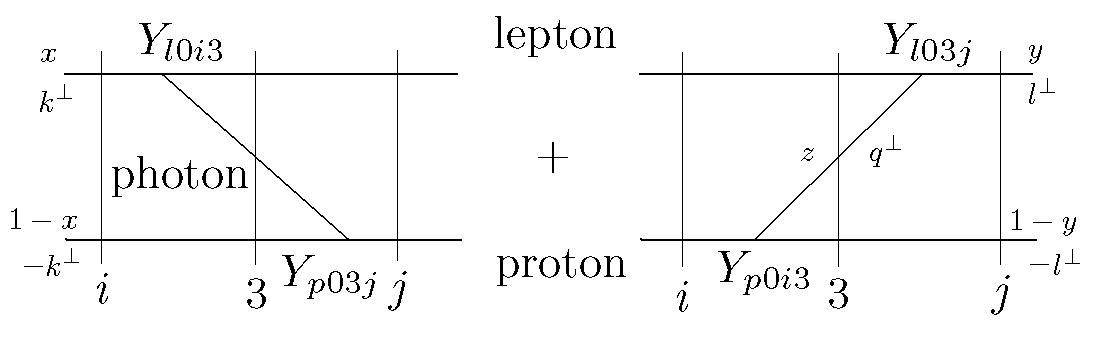
Figure 2: Exchange of the effective photon between the effective lepton and proton.

The operators $\hat{Y}_{0}(q_{t})$ involve the fermion terms that are obtained from Eq. (157) by putting the operators $q_{t}$ in place of $q_{0}$. Since anti-fermions do not contribute, the relevant operators $\hat{Y}_{n0}(q_{t})$ with $n=l,p$ are

$$\hat{Y}_{n0} = -\sum_{s_{1}s_{2}}\int_{p_{1}p_{2}q}\sqrt{\Delta(p_{1})\Delta(p_{2})\Delta(q)}\ \sqrt{2p_{1}^{+}p_{2}^{+}}\ \hat{Y}_{n}\,,$$ (188)

where $\hat{Y}_{n}$ involves only operators and masses for fermions number $n$, in the common pattern exhibited by the first four terms in Eq. (157).

The FF instantaneous interaction term whose matrix elements appear in Eq. (55) in addition to the photon exchange, $\hat{X}_{0}(q_{t})$, contains the fermion-fermion terms obtained from Eq. (169) by putting $q_{t}$ in place of $q_{0}$. The relevant part of $\hat{X}_{0}(q_{t})$ for the matrix elements $X_{0ij}$ in Eq. (55) is

$$\hat{X}_{0} = \sum_{n,l=1}^{2}\sum_{s_{1}s_{2}s_{3}s_{4}}\int_{p_{1}p_{2}p_{3}p_{4}}\,\sqrt{\Delta(p_{1})\Delta(p_{2})\Delta(p_{3})\Delta(p_{4})}\ \tilde{\delta}\ \sqrt{p_{1}^{+}p_{2}^{+}p_{3}^{+}p_{4}^{+}}\ {2\Delta(p_{4}-p_{3})\over(p_{4}^{+}-p_{3}^{+})^{2}}\ \hat{X}_{4nlA}\ ,$$ (189)

where

$$\hat{X}_{4nlA} = -(1-\delta_{nl})\ \delta_{s_{1}s_{2}}\delta_{s_{3}s_{4}}\ b_{ntp_{1}s_{1}}^{\dagger}b_{ltp_{3}s_{3}}^{\dagger}b_{ntp_{2}s_{2}}b_{ltp_{4}s_{4}}\ .$$ (190)

No other operators than $Y$ and $X$ are needed in the evaluation of the lepton-proton interaction in the lepton-proton bound-state eigenvalue equation up to $e^{2}$ in the formal series expansion in powers of $e$ in the RGPEP.

The matrix elements in Eq. (55) are

$$Y_{ij} = Y_{l0i3}Y_{p03j}+Y_{p0i3}Y_{l03j}\,=\,\langle i|\hat{Y}_{l0}\hat{Y}_{p0}+\hat{Y}_{p0}\hat{Y}_{l0}|j\rangle\,,$$ (191)

$$X_{ij} = \langle i|\hat{X}_{0}|j\rangle\,,$$ (192)

where the states $|i\rangle$ and $|j\rangle$ are created from vacuum by the effective lepton and proton creation operators. For example,

$$|i\rangle = b^{\dagger}_{lt\,ls}b^{\dagger}_{pt\,pr}|0\rangle\ .$$ (193)

Evaluation of $Y_{ij}$ and $X_{ij}$ proceeds using parameterization of momenta in Fig. 2,

$$l_{i}^{+} = xP^{+}\,,\quad\quad l_{i}^{\perp}\,=\,xP^{\perp}+k^{\perp}\,,$$ (194)

$$l_{j}^{+} = yP^{+}\,,\quad\quad l_{j}^{\perp}\,=\,yP^{\perp}+l^{\perp}\,,$$ (195)

$$p_{i}^{+} = (1-x)P^{+}\,,\quad\quad p_{i}^{\perp}\,=\,(1-x)P^{\perp}-k^{\perp}\,,$$ (196)

$$p_{j}^{+} = (1-y)P^{+}\,,\quad\quad p_{j}^{\perp}\,=\,(1-y)P^{\perp}-l^{\perp}\,,$$ (197)

$$q^{+} = zP^{+}\,,\quad\quad q^{\perp}\,=\,zP^{\perp}+\kappa^{\perp}\,,$$ (198)

where $P^{+}$ and $P^{\perp}$ denote the total momentum of the fermions. The total momentum is conserved by the interactions.

C.1 Evaluation of $Y_{ij}$

In evaluating a matrix element of a product of two $\hat{Y}$s, one for a lepton and one for a proton, one has to remember that one of the creation operators for one kind of fermions has to be commuted through the product of two operators of the other kind of fermions, with no net change of sign. The result for $Y_{ij}$ has the form

$$Y_{ij} = \sqrt{\Delta(p_{i})\Delta(p_{j})\Delta(l_{i})\Delta(l_{j})}\ \Delta(q)\ \sqrt{4p_{i}^{+}p_{j}^{+}l_{i}^{+}l_{j}^{+}}\ \tilde{\delta}\ \tilde{Y}_{ij}/q^{+}\,,$$ (199)

where

$$\tilde{Y}_{ij} = \theta(l_{i}^{+}-l_{j}^{+})\left[c(l_{i},s_{i},l_{j},s_{j})+m_{l}d(l_{i},s_{i},l_{j},s_{j})\right]\left[c^{*}(p_{i},-r_{i},p_{j},-r_{j})-m_{p}d(p_{i},-r_{i},p_{j},-r_{j})\right]$$ (200)

$$+ \theta(l_{i}^{+}-l_{j}^{+})\left[c^{*}(l_{i},-s_{i},l_{j},-s_{j})-m_{l}d(l_{i},-s_{i},l_{j},-s_{j})\right]\left[c(p_{i},r_{i},p_{j},r_{j})+m_{p}d(p_{i},r_{i},p_{j},r_{j})\right]$$

$$+ \theta(l_{j}^{+}-l_{i}^{+})\left[c(p_{i},r_{i},p_{j},r_{j})+m_{p}d(p_{i},r_{i},p_{j},r_{j})\right]\left[c^{*}(l_{i},-s_{i},l_{j},-s_{j})-m_{l}d(l_{i},-s_{i},l_{j},-s_{j})\right]$$

$$+ \theta(l_{j}^{+}-l_{i}^{+})\left[c^{*}(p_{i},-r_{i},p_{j},-r_{j})-m_{p}d(p_{i},-r_{i},p_{j},-r_{j})\right]\left[c(l_{i},s_{i},l_{j},s_{j})+m_{l}d(l_{i},s_{i},l_{j},s_{j})\right]$$

$$= \theta(l_{i}^{+}-l_{j}^{+})\ Y_{+}+\theta(l_{j}^{+}-l_{i}^{+})\ Y_{-}\,,$$ (201)

and

$$c(l_{i},s_{i},l_{j},s_{j}) = \left[\left({l_{j}\over l_{j}^{+}}-{q\over q^{+}}\right)\,\delta_{s_{i}1}\delta_{s_{j}1}+\left({l_{i}\over l_{i}^{+}}-{q\over q^{+}}\right)\,\delta_{s_{j}-1}\delta_{s_{i}-1}\right]\,,$$ (202)

$$d(l_{i},s_{i},l_{j},s_{j}) = \left({1\over l_{j}^{+}}-{1\over l_{i}^{+}}\right)\delta_{s_{i}1}\delta_{s_{j}-1}\,,$$ (203)

$$c(p_{i},r_{i},p_{j},r_{j}) = \left[\left({p_{j}\over p_{j}^{+}}-{q\over q^{+}}\right)\,\delta_{r_{i}1}\delta_{r_{j}1}+\left({p_{i}\over p_{i}^{+}}-{q\over q^{+}}\right)\,\delta_{r_{j}-1}\delta_{r_{i}-1}\right]\,,$$ (204)

$$d(p_{i},r_{i},p_{j},r_{j}) = \left({1\over p_{j}^{+}}-{1\over p_{i}^{+}}\right)\delta_{r_{i}1}\delta_{r_{j}-1}\,.$$ (205)

To explain how the calculation proceeds, it is enough to show details for $Y_{+}$, which is

$$P^{+\,2}\ Y_{+} = \ \delta_{s_{i}1}\delta_{s_{j}1}\ \delta_{r_{i}-1}\delta_{r_{j}-1}\ \left[\left({l\over y}-{\kappa\over z}\right)\left({-l^{*}\over 1-y}-{\kappa^{*}\over z}\right)+\left({k^{*}\over x}-{\kappa^{*}\over z}\right)\left({-k\over 1-x}-{\kappa\over z}\right)\right]$$ (206)

$$+ \delta_{s_{i}1}\delta_{s_{j}1}\ \delta_{r_{i}1}\delta_{r_{j}1}\ \left[\left({l\over y}-{\kappa\over z}\right)\left({-k^{*}\over 1-x}-{\kappa^{*}\over z}\right)+\left({k^{*}\over x}-{\kappa^{*}\over z}\right)\left({-l\over 1-y}-{\kappa\over z}\right)\right]$$

$$+ \delta_{s_{i}-1}\delta_{s_{j}-1}\ \delta_{r_{i}-1}\delta_{r_{j}-1}\ \left[\left({k\over x}-{\kappa\over z}\right)\left({-l^{*}\over 1-y}-{\kappa^{*}\over z}\right)+\left({l^{*}\over y}-{\kappa^{*}\over z}\right)\left({-k\over 1-x}-{\kappa\over z}\right)\right]$$

$$+ \delta_{s_{i}-1}\delta_{s_{j}-1}\ \delta_{r_{i}1}\delta_{r_{j}1}\ \left[\left({k\over x}-{\kappa\over z}\right)\left({-k^{*}\over 1-x}-{\kappa^{*}\over z}\right)+\left({l^{*}\over y}-{\kappa^{*}\over z}\right)\left({-l\over 1-y}-{\kappa\over z}\right)\right]$$

$$+ \delta_{s_{i}1}\delta_{s_{j}1}\ \delta_{r_{i}-1}\delta_{r_{j}1}\ \left({l\over y}-{\kappa\over z}\right)\,{m_{p}z\over(1-y)(1-x)}\,$$

$$+ \delta_{s_{j}1}\delta_{s_{i}1}\ \delta_{r_{i}1}\delta_{r_{j}-1}\ \left({k^{*}\over x}-{\kappa^{*}\over z}\right)\,{-m_{p}z\over(1-y)(1-x)}\,$$

$$+ \delta_{s_{i}-1}\delta_{s_{j}-1}\ \delta_{r_{i}-1}\delta_{r_{j}1}\left({k\over x}-{\kappa\over z}\right)\,{m_{p}z\over(1-y)(1-x)}\,$$

$$+ \delta_{s_{i}-1}\delta_{s_{j}-1}\ \delta_{r_{i}1}\delta_{r_{j}-1}\left({l^{*}\over y}-{\kappa^{*}\over z}\right)\,{-m_{p}z\over(1-y)(1-x)}\,$$

$$+ \delta_{s_{i}1}\delta_{s_{j}-1}\ \delta_{r_{i}-1}\delta_{r_{j}-1}\,{m_{l}z\over xy}\,\left({-l^{*}\over 1-y}-{\kappa^{*}\over z}\right)$$

$$+ \delta_{s_{j}1}\delta_{s_{i}-1}\ \delta_{r_{j}1}\delta_{r_{i}1}\,{m_{l}z\over xy}\,\left({-k^{*}\over 1-x}-{\kappa^{*}\over z}\right)$$

$$+ \delta_{s_{i}-1}\delta_{s_{j}1}\ \delta_{r_{i}1}\delta_{r_{j}1}\,{m_{l}z\over xy}\,\left({l\over 1-y}+{\kappa\over z}\right)$$

$$+ \delta_{s_{i}-1}\delta_{s_{j}1}\ \delta_{r_{j}-1}\delta_{r_{i}-1}\,{m_{l}z\over xy}\,\left({k\over 1-x}+{\kappa\over z}\right)$$

$$+ \left(\delta_{s_{i}1}\delta_{s_{j}-1}\ \delta_{r_{i}-1}\delta_{r_{j}1}+\delta_{s_{i}-1}\delta_{s_{j}1}\ \delta_{r_{i}1}\delta_{r_{j}-1}\right){m_{l}m_{p}z^{2}\over x(1-x)\,y(1-y)}\,.$$

One can obtain this result using free spinors with physical fermion masses in the fermion currents and contracting the Lorentz indices of the currents with the indices of the tensor that results from the sum over polarizations of the transverse photons exchanged between fermions. Therefore, this result can be arrived at using the canonical QFT irrespective of the difference between the bare and effective particles.

Since the same type of analysis applies to all terms in $Y$, we explicitly consider only the first spin amplitude

$$A_{1} = \delta_{s_{i}1}\delta_{s_{j}1}\ \delta_{r_{i}-1}\delta_{r_{j}-1}B_{1}\,,$$ (207)

where

$$B_{1} = \left({l\over y}-{\kappa\over z}\right)\left({-l^{*}\over 1-y}-{\kappa^{*}\over z}\right)+\left({k^{*}\over x}-{\kappa^{*}\over z}\right)\left({-k\over 1-x}-{\kappa\over z}\right)$$ (208)

$$= {2|\kappa|^{2}\over z^{2}}+{x+y-1\over z}\ \left[{|k|^{2}\over x(1-x)}-{|l|^{2}\over y(1-y)}\right]-{lk^{*}\over xy}-{l^{*}k\over(1-x)(1-y)}\,.$$ (209)

The first term in $B_{1}$ behaves as $1/z^{2}$ for small $z$, the second term as $1/z$, and the third term is regular. Only the terms that do not change fermion spins involve $1/z^{2}$. The most singular for small $z$ terms appear only in the first four spin amplitudes in $Y_{+}$. Therefore, they provide the leading behavior of the entire $Y_{+}$ for small values of $z$,

$$P^{+\,2}\ Y_{+} = \delta_{s_{i}s_{j}}\ \delta_{r_{i}r_{j}}\ 2(k^{\perp}-l^{\perp})^{2}/z^{2}\,.$$ (210)

It is these leading terms that count most in the formation of lepton-proton bound states for small electric charge $e$ in the presence of the RGPEP form factors in Eqs. (52) and (53). The reason is that the form factors are order 1 when the invariant mass differences in denominators in Eqs. (52) and (53) are small and the same form factors are exponentially small when the changes of the invariant masses of fermion states are large. The lepton momentum fractions $x$ and $y$ must be close to the ratio of the lepton mass to the sum of lepton and proton masses and cannot change much because this would create a large change in the invariant mass and thus also the large differences in the denominators and form factors’ arguments. On the other hand, photons are massless and can carry small fractions $z$ if their $q^{\perp}$s are sufficiently small not to cause large invariant mass changes. This is what happens in the atomic-like bound states.

The evaluation of $Y_{-}$ in Eq. (201) yields the same result as Eq. (210). Therefore, Eqs. (199) and (201) together yield

$$Y_{ij} = \sqrt{\Delta(p_{i})\Delta(p_{j})\Delta(l_{i})\Delta(l_{j})}\ \Delta(q)\ \sqrt{4p_{i}^{+}p_{j}^{+}l_{i}^{+}l_{j}^{+}}\ \tilde{\delta}\ {\delta_{s_{i}s_{j}}\ \delta_{r_{i}r_{j}}\ 2(k^{\perp}-l^{\perp})^{2}\over q^{+\,3}}\,.$$ (211)

In the limit of removing the regularization,

$$Y_{ij} = \sqrt{4p_{i}^{+}p_{j}^{+}l_{i}^{+}l_{j}^{+}}\ \tilde{\delta}\ {\delta_{s_{i}s_{j}}\ \delta_{r_{i}r_{j}}\ 2(k^{\perp}-l^{\perp})^{2}\over q^{+\,3}}\,.$$ (212)

Writing $l_{i}+=xP^{+}$ and $l_{j}^{+}=yP^{+}$, one arrives at

$$Y_{ij} = \sqrt{x(1-x)y(1-y)}\ P^{+\,2}\ \tilde{\delta}\ {\delta_{s_{i}s_{j}}\ \delta_{r_{i}r_{j}}\ 4(k^{\perp}-l^{\perp})^{2}\over q^{+\,3}}\,.$$ (213)

C.2 Evaluation of $X_{ij}$

In evaluating the matrix elements of $\hat{X}_{4nlA}$, one has to take into account that one creation operator for one kind of fermions has to be commuted through one creation operator of the other kind of fermions, with net result of a change of sign. The matrix element $X_{ij}$ includes the sum of a term with $n=l$ and $l=p$ and a term with $n=p$ and $l=n$. In the case of $l_{i}^{+}>l_{j}^{+}$, which corresponds to evaluation of $Y_{+}$ in App. C.2, one has to consider only terms that result from the absorption of a photon by the lepton,

$$X_{ij} = (-1)\sqrt{\Delta(p_{i})\Delta(p_{j})\Delta(l_{i})\Delta(l_{j})}\ \Delta(q)\ \sqrt{p_{i}^{+}p_{j}^{+}l_{i}^{+}l_{j}^{+}}\ \tilde{\delta}\ {-4\delta_{s_{i}s_{j}}\delta_{r_{i}r_{j}}\ \over q^{+\,2}}\ .$$ (214)

The result for $Y_{-}$ is the same. After removal of regularization one has

$$X_{ij} = \sqrt{p_{i}^{+}p_{j}^{+}l_{i}^{+}l_{j}^{+}}\ \tilde{\delta}\ {4\delta_{s_{i}s_{j}}\delta_{r_{i}r_{j}}\ \over q^{+\,2}}\ .$$ (215)

Using the same parameterization of $l_{i}^{+}$ and $l_{j}^{+}$ as in Eq. (213), one obtains

$$X_{ij} = \sqrt{x(1-x)y(1-y)}\ P^{+\,2}\ \tilde{\delta}\ {4\delta_{s_{i}s_{j}}\delta_{r_{i}r_{j}}\ \over q^{+\,2}}\ .$$ (216)

C.3 Evaluation of ${\cal F}_{ij\,\rm int}$ and ${\cal F}_{ij\,\rm cor}$

The denominators to consider are $i3=-3i$ and $j3=-3j$. In both diagrams in Fig. 2 the calculation is carried out in the same fashion. In the case of the left diagram,

$$p_{i3}/i3 = -q^{+}\,\left[\kappa^{\perp\,2}+{m_{l}^{2}z^{2}\over xy}+\left({l^{\perp\,2}\over y}-{k^{\perp\,2}\over x}\right)z\right]^{-1}\,,$$ (217)

$$p_{j3}/j3 = -q^{+}\left[\kappa^{\perp\,2}+{m_{p}^{2}z^{2}\over(1-x)(1-y)}+\left({k^{\perp\,2}\over 1-x}-{l^{\perp\,2}\over 1-y}\right)z\right]^{-1}\,.$$ (218)

In the square brackets, the first two terms dominate for small $z$ and transverse momenta much smaller than the fermion masses. These conditions are secured in the case of small mass eigenstates of the full eigenvalue problem by the presence of RGPEP vertex form factors $f$ with large effective particle size $s$. The lepton momentum fractions $x$ and $y$ in the effective lepton-proton Fock sector are approximately

$$\beta = m_{l}/(m_{l}+m_{p})\,,$$ (219)

and in the leading approximation for transverse momenta much smaller than masses and for $x$ and $y$ close to $\beta$, one has

$$p_{i3}/i3 = p_{j3}/j3\,=\,-q^{+}\left[(k^{\perp}-l^{\perp})^{2}+(m_{l}+m_{p})^{2}z^{2}\right]^{-1}\,.$$ (220)

This result says that $i3$ and $j3$ for finite fermion momenta $p_{i3}$ and $p_{j3}$, behave as the photon $q^{-}$ on mass shell plus a correction due to the $+$ momentum carried by the photon. Thus, these denominators diverge when $z\to 0$ for fixed $|k^{\perp}-l^{\perp}|$.

At the same time,

$$ij = {|k|^{2}\over x(1-x)}-{|l|^{2}\over y(1-y)}+{m_{l}^{2}\over x}+{m_{p}^{2}\over 1-x}-{m_{l}^{2}\over y}-{m_{p}^{2}\over 1-y}\,,$$ (221)

which is finite for small $z$ and vanishes for vanishing $z$ and $|k^{\perp}-l^{\perp}|$. Therefore, one can neglect $ij$ in comparison to $i3$ and $j3$. Consequently, ${\cal F}_{ij\,\rm int}$ in Eq. (52) reduces to

$${\cal F}_{ij\,\rm int} = -q^{+}\left[(k^{\perp}-l^{\perp})^{2}+(m_{l}+m_{p})^{2}z^{2}\right]^{-1}\,.$$ (222)

This result completes calculation of ${\cal F}_{ij\,\rm int}$.

Evaluation of ${\cal F}_{ij\,\rm cor}$ in Eq. (53) now only requires estimates of $f_{i3}$ and $f_{3j}$ in

$${\cal F}_{ij\,\rm cor} = (1-f_{ij})\ f_{i3}f_{3j}\ {-q^{+}\over(k^{\perp}-l^{\perp})^{2}+(m_{l}+m_{p})^{2}z^{2}}\,,$$ (223)

where $(p_{i3}/i3+p_{3j}/j3)/2$ is approximated using Eq. (220). The same approximation yields the arguments $i3$ and $j3$ of $f$ in the form

$$i3 = {\beta\over z}\ \left[(k^{\perp}-l^{\perp})^{2}+(m_{l}+m_{p})^{2}z^{2}\right]\ ,$$ (224)

$$j3 = {1-\beta\over z}\ \left[(k^{\perp}-l^{\perp})^{2}+(m_{l}+m_{p})^{2}z^{2}\right]\ .$$ (225)

Analogous reasoning applies in the case of $Y_{-}$. The point is that the form factors $f_{i3}$ and $f_{3j}$ vanish exponentially fast for small values of $z$, where the dominant interaction is active. Therefore, ${\cal F}_{ij\,\rm cor}$ is neglected in comparison with ${\cal F}_{ij\,\rm int}$ in Eq. (51).

Appendix D Integration in $d_{f}$ and $d_{a}$

Integration in Eq. (115) must be carried out numerically, but it is useful to simplify the six-dimensional integral. For the $s$-wave ground state one has

$$d_{f} = {2\int d^{3}p\int d^{3}p\,^{\prime}\ \ {1\over(1+p^{2})^{2}}\ \left[e^{-4\alpha^{4}(p^{2}-p\,^{\prime 2})^{2}/a^{4}}-1\right]\ {4\pi\over(\vec{p}-\vec{p}\,^{\prime})^{2}}\ {1\over(1+p\,^{\prime 2})^{2}}\over(2\pi)^{3}\int d^{3}p\ {1\over(1+p^{2})^{4}}}\ .$$ (226)

The $z$-axis in integration over $\vec{p}\,^{\prime}$ can be chosen along $\vec{p}$. Integration over angles of $\vec{p}\,^{\prime}$ replaces $1/\vec{q}\,^{2}$ by

$${\pi\over pp^{\prime}}\ \ln{(p+p^{\prime})^{2}\over(p-p^{\prime})^{2}}\ .$$ (227)

There is no dependence left on angles of $\vec{p}$. So, integration over all angles yields

$$d_{f} = {2\cdot 4\pi\ {\pi\cdot 4\pi}\over(2\pi)^{3}4\pi\cdot\pi/32}\ \int_{0}^{\infty}pdp\int_{0}^{\infty}p^{\prime}dp^{\prime}\ {e^{-4\alpha^{4}(p^{2}-p\,^{\prime 2})^{2}/a^{4}}-1\over(1+p^{2})^{2}(1+p^{\prime}\,{}^{2})^{2}}\ \ \ln{(p+p^{\prime})^{2}\over(p-p^{\prime})^{2}}\ .$$ (228)

Introducing variables $u=p^{2}$ and $v=p^{\prime}\,{}^{2}$, one obtains

$$d_{f} = {32\over\pi^{2}}\ \int_{0}^{\infty}du\int_{0}^{u}dv\ \ {e^{-z^{2}(u-v)^{2}}-1\over(1+u)^{2}(1+v)^{2}}\ \ \ln{\sqrt{u}+\sqrt{v}\over\sqrt{u}-\sqrt{v}}\ ,$$ (229)

where

$$z^{2} = 2(\alpha/a)^{2}\ .$$ (230)

If the parameter $a$ changes from $1/20$ to 3, the parameter $z$ changes between $8\ 10^{2}\alpha^{2}$ and $(2/9)\alpha^{2}$. Changing variables to $zu$ and $zv$, one has

$$d_{f\,S1} = {32\over\pi^{2}}\ z^{2}\ \int_{0}^{\infty}du\int_{0}^{u}dv\ \ {e^{-(u-v)^{2}}-1\over(z+u)^{2}(z+v)^{2}}\ \ \ln{\sqrt{u}+\sqrt{v}\over\sqrt{u}-\sqrt{v}}\ .$$ (231)

References

• (1) E. E. Salpeter, H. A. Bethe, Phys. Rev. 84, 1232 (1951).
• (2) M. Gell-Mann, F. Low, Phys. Rev. 84, 350 (1951).
• (3) H. Bethe and E. Salpeter, Quantum Mechanics of One- and Two-Electron Atoms Plenum Press (New York, 1977).
• (4) W. E. Caswell, G. P. Lepage, Phys. Lett. B 167, 437 (1986).
• (5) Quantum Electrodynamics, Ed. T. Kinoshita (World Scientifc, Singapore, 1990).
• (6) T. Kinoshita, M. Nio, Phys. Rev. Lett. 82, 3240 (1999), Erratum-ibid. 103, 07990 (2009).
• (7) K. Pachucki, Phys. Rev A 60, 3593 (1999).
• (8) K. Pachucki, Phys. Rev. A 71, 012503 (2005).
• (9) B. D. Jones, R. J. Perry, Phys. Rev. D 55, 7715 (1997).
• (10) T. Aoyama, M. Hayakawa, T. Kinoshita, M. Nio, Phys. Rev. Lett. 109, 111808 (2012).
• (11) P. J. Mohr, B. N. Taylor, D. B. Newell, Rev. Mod. Phys. 84, 1527 (2012).
• (12) R. Pohl, R. Gilman, G. A. Miller, K. Pachucki, Ann. Rev. Nucl. Part. Sci. 63, 175 (2013).
• (13) S. D. Głazek, Acta Phys. Pol. B 43, 1843 (2012).
• (14) P. A. M. Dirac, Rev. Mod. Phys. 21, 392 (1949).
• (15) J. C. Bernauer et al., Phys. Rev. Lett. 105, 242001 (2010).
• (16) R. Pohl et al., Nature 466, 213 (2010).
• (17) S. D. Głazek, K. G. Wilson Phys. Rev. D 48, 5863 (1993).
• (18) S. D. Głazek, K. G. Wilson Phys. Rev. D 49, 4214 (1994).
• (19) S. D. Głazek, in Theory of Hadrons and Light-Front QCD, World Scientific (Singapore, 1995); p. 208.
• (20) S. D. Głazek, Acta Phys. Pol. B 29, 1979 (1998).
• (21) F. Wegner, Ann. Phys. (Berlin) 506, 77 (1994).
• (22) K. G. Wilson et al., Phys. Rev. D 49, 6720 (1994).
• (23) S. D. Głazek, Phys. Rev. D 69, 065002 (2004).
• (24) C. D. Roberts, A. G. Williams, Prog. Part. Nucl. Phys. 33, 477 (1994).
• (25) C. Bloch, Nucl. Phys. 6, 329 (1958).
• (26) K. G. Wilson Phys. Rev. D 2, 1438 (1970).
• (27) S. D. Głazek, Acta Phys. Polon. B 42, 1933 (2011).
• (28) G. F. de Teramond, S. J. Brodsky, Phys. Rev. Lett. 94, 201601 (2005),
• (29) J. M. Maldacena, Adv. Theor. Math. Phys. 2, 231 (1998).
• (30) E. Schrödinger, Ann. Phys. 79, 361 (1926).
• (31) S. D. Głazek, A. P. Trawiński, Phys. Rev. D 88, 105025 (2013).
• (32) S. D. Głazek, J. Młynik Phys. Rev. D 67, 045001 (2003).
• (33) T.-M. Yan, Phys. Rev. D 7, 1780 (1973).
• (34) M. Gell-Mann, M.L. Goldberger Phys. Rev. 91, 398 (1953).
• (35) S. D. Głazek, Phys. Rev. D 87, 125032 (2013).
• (36) E. A. Bartnik, S. D. Głazek, Phys. Rev. D 39, 1249 (1989).