MODERN GEOMETRY IN NOT-SO-HIGH ECHELONS OF PHYSICS:
CASE STUDIES

Abstract

In this mostly pedagogical tutorial article a brief introduction to modern geometrical treatment of fluid dynamics and electrodynamics is provided. The main technical tool is standard theory of differential forms. In fluid dynamics, the approach is based on general theory of integral invariants (due to Poincaré and Cartan). Since this stuff is still not considered common knowledge, the first chapter is devoted to an introductory and self-contained exposition of both Poincaré version as well as Cartan’s extension of the theory. The main emphasis in fluid dynamics part of the text is on explaining basic classical results on vorticity phenomenon (vortex lines, vortex filaments etc.) in ideal fluid. In electrodynamics part, we stress the aspect of how different (in particular, rotating) observers perceive the same space-time situation. Suitable $3+1$ decomposition technique of differential forms proves to be useful for that. As a representative (an simple) example we analyze Faraday’s law of induction (and explicitly compute the induced voltage) from this point of view.

261359 Department of Theoretical Physics and Didactics of Physics,
Comenius University, Bratislava, Slovakia

KEYWORDS:

Ideal fluid, barotropic flow, vortex lines, transport theorem, Helmholtz theorem, lines of solenoidal field, integral invariant, 3+1 decomposition, rotating frame, Faraday’s law

1 Introduction

Among theoretical physicists, modern differential geometry is typically associated with its “higher echelons”, like advanced general relativity, string theory, topologically non-trivial solutions in gauge theories, Kaluza-Klein theories and so on.

However, geometrical methods also proved to be highly effective in several other branches of physics which are usually treated as more “mundane” or, put it differently, as “not-so-high echelons” of theoretical physics. Good old fluid dynamics (or, more generally, dynamics of continuous media) and electrodynamics may serve as prominent examples.

Nowadays, some education in modern differential geometry (manifolds, differential forms, Lie derivatives, …) becomes a standard part of theoretical physics curriculum. After learning those things, however, the potential strength of this mathematics is rarely demonstrated in real physics courses.

Although I definitely do not advocate entering of modern geometry into “first round” physics courses (of, say, above mentioned fluid dynamics and electrodynamics), it seems to me that to show how it is really used in some “second round” courses might be quite a good idea. First, in this way some more advanced material in the particular subject may be explained in a simple and lucid way so typical for modern geometry. Second, from the opposite perspective, this exposition is the best way to show how differential geometry itself really works.

If, on the contrary, this is not done so, modern geometry is segregated from real life and forced out to the above mentioned “higher echelons”, with the natural consequence that for majority of students who put considerable energy into grasping this stuff in mathematics courses all their work is completely in vain.

Now, a few words about the structure of this tutorial article.

In the fluid dynamics part, we restrict to ideal (inviscid) fluid and, in addition, are only interested in the barotropic case (except for Ertel’s theorem, which is more general). Our exposition rests on theory of integral invariants due to Poincaré and Cartan. I think this approach is well suited for treating classical material concerning vorticity (like Helmholtz and Kelvin’s theorems). Perhaps it is worth noting that we treat fluid dynamics in terms of “extended” space as the underlying manifold (i.e. the space where time is a full-fledged dimension rather than just a parameter).

In electrodynamics part, we first derive Maxwell equations in terms of differential forms in 4-dimensional space-time (this is achieved by learning the structure of general forms in Minkowski space and checking it versus the standard 3-dimensional version of the equations). Then, in the second step, we introduce the concept of observer field in space-time, intimately connected to the concept of reference frame. Using appropriate technique of 3+1 (space + time) decomposition of forms (and operations on them) with respect to the observer field we can easily compute what various observers “see” when they “look at invariant space-time electromagnetic reality”. As an elementary example of this approach, we explicitly compute relativistically induced electric field seen in the rotating frame of a wire rim as well as its line integral along the rim (the induced voltage) in the Faraday’s law demonstration setting.

The reader is supposed to have basic working knowledge of modern geometry mentioned above (manifolds, differential forms, Lie derivatives, …; if not, perhaps the crash course [Fecko 2007] might help as a first aid treatment). More tricky material is explained in the text (and mostly a detailed computation is given when needed).

In Appendix A we collect useful formulas which relate expressions in the language of differential forms in 3-dimensional Euclidean space (as well as 4-dimensional Minkowski space) to their counterparts from usual vector analysis. Ability to translate various expressions from one language to another (go back and forth at any moment) is essential for effective use of forms in both fluid dynamics and electrodynamics.

Appendices B and C are devoted to answering the question whether field lines of solenoidal (divergence-free) vector field indeed cannot end (or start) inside the domain where there are defined (they can :-).

2 Integral invariants - what Poincaré and what Cartan

2.1 Motivation - why the topic appears here

Theory of integral invariants is a well-established part of geometry with various applications. It is probably best-known from Hamiltonian mechanics.

Integral invariants were first formally introduced and studied by Poincaré in his celebrated memoir [Poincaré 1890]. He explained them in more detail in the book [Poincaré 1899]. Then the concept was developed by Cartan and summarized in his monograph [Cartan 1922].

What was Cartan’s contribution? Roughly speaking, while Poincaré considered invariants in phase space, Cartan studied these objects in extended phase space. This led him to a true generalization: one can associate, with each Poincaré invariant, corresponding Cartan’s invariant. The latter proves to be invariant with respect to a “wider class of operations” (see more below). In addition, and this point of view will be of particular interest for us, going from Poincaré version to Cartan’s one may be regarded, in a sense, as going from time-independent situation to time-dependent one.

Since the theory of integral invariants is both instructive in its own right and used in Chapter 3, we placed it in the very beginning of the paper.

In Chapter 3, we first use its original Poincaré version in Section 3.2 and then, already the Cartan’s extension, as a tool providing non-stationary fluid dynamics equations from the known form of the stationary case in Sec 3.3 and for gaining useful information from it in Sec. 3.4.

Remarkably, if we do it in this way, the resulting more general non-stationary equation looks simpler than the stationary one. In addition, its consequences, like Helmholtz theorem on behavior of vortex lines in inviscid fluid, look very naturally in this picture.

2.2 Poincaré

Let’s start with Poincaré invariants.

Consider a manifold $M$ endowed with dynamics given by a vector field $v$

$$\dot{\gamma}=v\hskip 42.67912pt{\dot{x}}^{i}=v^{i}(x)$$ (2.2.1)

The field $v$ generates the dynamics (time evolution) via its flow $\Phi_{t}\leftrightarrow v$. We will call the structure phase space

$$(M,\Phi_{t}\leftrightarrow v)\hskip 28.45274pt\text{{\color[rgb]{1,0,0}\emph{phase space}}}$$ (2.2.2)

In this situation, let’s have a $k$-form $\alpha$ and consider its integrals over various $k$-chains ($k$-dimensional surfaces) $c$ on $M$. Due to the flow $\Phi_{t}$ corresponding to $v$, the $k$-chains flow away, $c\mapsto\Phi_{t}(c)$. Compare the value of integral of $\alpha$ over the original $c$ and integral over $\Phi_{t}(c)$. If, for any chain $c$, the two integrals are equal, it clearly reflects a remarkable property of the form $\alpha$ with respect to the field $v$. We call it integral invariant:

$$\int_{\Phi_{t}(c)}\alpha=\int_{c}\alpha\hskip 28.45274pt\Leftrightarrow\hskip 28.45274pt\int_{c}\alpha\ \ \ \text{is {\color[rgb]{1,0,0}\emph{integral invariant}}}$$ (2.2.3)

Let’s see what this says for infinitesimal $t\equiv\epsilon$. Then

$$\int_{\Phi_{\epsilon}(c)}\alpha=\int_{c}\alpha+\epsilon\int_{c}\mathcal{L}_{v}\alpha$$ (2.2.4)

(plus, of course, higher order terms in $\epsilon$; here $\mathcal{L}_{v}$ is Lie derivative along $v$). So, in the case of integral invariant, the condition

$$\int_{c}\mathcal{L}_{v}\alpha=0$$ (2.2.5)

is to be fulfilled. Since this is to be true for each $c$, the form (under the integral sign) itself in (2.2.5) is to vanish

$$\mathcal{L}_{v}\alpha=0$$ (2.2.6)

This is the differential version of the statement (2.2.3).

There is, however, an important subclass of $k$-chains, namely $k$-cycles. These are chains whose boundary vanish:

$$\partial c=0\hskip 56.9055ptc=\ \text{\emph{cycle}}$$ (2.2.7)

In specific situations, it may be enough that some integral only behaves invariantly when restricted to cycles. If this is the case, the condition (2.2.6) is overly strong. It can be weakened to the requirement that the form under the integral sign in (2.2.5) is exact, i.e.

$$\mathcal{L}_{v}\alpha=d\tilde{\beta}$$ (2.2.8)

for some form $\tilde{\beta}$.

$\blacktriangledown\hskip 14.22636pt$ Indeed, in one direction, Eqs. (2.2.7) and (2.2.8) then give

$$\int_{c}\mathcal{L}_{v}\alpha=\int_{c}d\tilde{\beta}=\int_{\partial c}\tilde{\beta}=0$$ (2.2.9)

so that (2.2.5) is fulfilled. In the opposite direction, if the integral (2.2.5) is to vanish for each cycle, the form under the integral sign is to be exact (due to de Rham theorem), so (2.2.8) holds. $\blacktriangle$

According to whether the integrals of forms are invariant for arbitrary $k$-chains or just for $k$-cycles, integral invariants are divided into absolute invariants (for any $k$-chains) and relative ones (just for $k$-cycles). We can summarize what we learned yet as follows:

$$\{\mathcal{L}_{v}\alpha=0,\ c\ \text{arbitrary}\} \Leftrightarrow \int_{c}\alpha\ \ \ \text{is {\it absolute} integral invariant}$$ (2.2.10)

$$\{\mathcal{L}_{v}\alpha=d\tilde{\beta},\ c=\ \text{cycle}\} \Leftrightarrow \oint_{c}\alpha\ \ \ \text{is {\it relative} integral invariant}$$ (2.2.11)

Let’s see, now, what else we can say about relative integral invariants. The condition (2.2.8) may be rewritten (using $\mathcal{L}_{v}=i_{v}d+di_{v}$) as

$$i_{v}d\alpha=d\beta$$ (2.2.12)

(where $\beta=\tilde{\beta}-i_{v}\alpha$). Therefore it holds, trivially,

$$i_{v}d\alpha=d\beta\hskip 28.45274pt\Leftrightarrow\hskip 28.45274pt\mathcal{L}_{v}\alpha=d\tilde{\beta}$$ (2.2.13)

and so also the following main statement on relative invariants (reformulation of (2.2.11)) is true:

$$\boxed{i_{v}d\alpha=d\beta\hskip 14.22636pt\Leftrightarrow\hskip 14.22636pt\mathcal{L}_{v}\alpha=d\tilde{\beta}\hskip 14.22636pt\Leftrightarrow\hskip 14.22636pt\oint_{c}\alpha=\ \ \text{\emph{relative} invariant}}$$ (2.2.14)

So we can identify the presence of relative integral invariant in differential version: on phase space $(M,v)$, we see a form $\alpha$ fulfilling any of the two equations mentioned in Eq. (2.2.13).

[Perhaps we should stress how the second equivalence sign is to be interpreted. There is no $\beta$ under the integral sign. Therefore, from the rightmost statement of Eq. (2.2.14), it is not possible to reconstruct any particular $\beta$, present in the leftmost statement. So one should read the second equivalence sign, in particular its right-to-left direction, as the assertion that, provided the rightmost statement holds, there exists a form $\beta$ such that the leftmost statement is true. (And, of course, one should adopt the same attitude with respect to the middle statement and $\tilde{\beta}$.)]

Notice that, as a consequence of Eq. (2.2.8), we also get the equation

$$\mathcal{L}_{v}(d\alpha)=0$$ (2.2.15)

This says, however (see Eq. (2.2.10)), that integral of $d\alpha$ is absolute integral invariant. So, if we find a relative invariant given by $\alpha$, then $d\alpha$ provides an absolute invariant:

$$\boxed{\oint_{c}\alpha\ \ \text{is relative invariant}\hskip 17.07182pt\Rightarrow\hskip 17.07182pt\int_{D}d\alpha\ \ \text{is absolute invariant}}$$ (2.2.16)

(here $\partial c=0$, whereas $\partial D$ may not vanish).

Conversely, if we find an absolute invariant then it is, clearly, also a relative one (if something is true for all chains then it is, in particular, true for closed chains, i.e. for cycles). Absolute invariants thus present a part (subset) of relative invariants and the exterior derivative $d$ maps relative invariants into absolute invariants.

[Notice that whenever we find a ”good” triple $(v,\alpha,\beta)$ (i.e. $i_{v}d\alpha=d\beta$ holds), we can generate, for the same dynamics $(M,v)$, a series of additional ”good” triples

$$(v,\alpha,\beta)_{\text{new}} \leftrightarrow (v,\alpha\wedge d\alpha,2\beta\wedge d\alpha)$$ (2.2.17)

$$\leftrightarrow (v,\alpha\wedge d\alpha\wedge d\alpha,3\beta\wedge d\alpha\wedge d\alpha)$$ (2.2.18)

$$\dots$$ (2.2.19)

$$\leftrightarrow (v,\alpha\wedge(d\alpha)^{k},(k+1)\beta\wedge(d\alpha)^{k}\hskip 28.45274ptk=0,1,2,\dots$$ (2.2.20)

(check) so that we get a series of relative invariants

$$\oint_{c_{(0)}}\alpha\hskip 19.91684pt\oint_{c_{(1)}}\alpha\wedge d\alpha\hskip 19.91684pt\dots\hskip 20.20164pt\oint_{c_{(k)}}\alpha\wedge(d\alpha)^{k}\hskip 19.91684ptk=0,1,2,\dots$$ (2.2.21)

(Here $c_{(k)}$ are cycles of appropriate dimensions. For deg $d\alpha$ = odd and $k\geq 2$ we get, clearly, vacuous statements, since $(d\alpha)^{k}=0$.)]

Example 2.2.1: Consider the Hamiltonian mechanics (the autonomous case, yet, i.e. with the Hamiltonian $H$ independent of time). Here the dynamical field $v$ is the Hamiltonian field $\zeta_{H}$ given by the equation

$$i_{\zeta_{H}}d\theta=-dH\hskip 28.45274pt\theta=p_{a}dq^{a}$$ (2.2.22)

(see Ch.14 in ([Fecko 2006])). Comparison with Eq. (2.2.12)

$$i_{\zeta_{H}}d\theta=-dH\hskip 28.45274pt\leftrightarrow\hskip 28.45274pti_{v}d\alpha=d\beta$$ (2.2.23)

reveals that a good $\alpha$ is the 1-form $\theta$. The role of the corresponding form $\beta$ (potential) is played by the (minus) Hamiltonian $H$.

[Notice that this property of $\theta$ is actually true w.r.t. the field $v=\zeta_{H}$ for arbitrary $H$, i.e. w.r.t. a whole family of dynamical fields on $M$. So, in this particular realization of the triple $(M,v,\alpha)$, a single $\alpha$ is good for a whole family of dynamical vector fields $v$ (namely, for all Hamiltonian fields).]

According to Eqs. (2.2.17) - (2.2.20), we have also additional triples $(v,\alpha,\beta)$, given as

$$(v,\alpha,\beta) \leftrightarrow (\zeta_{H},\theta,-H)$$ (2.2.24)

$$\leftrightarrow (\zeta_{H},\theta\wedge\omega,-2H\omega)$$ (2.2.25)

$$\leftrightarrow (\zeta_{H},\theta\wedge\omega\wedge\omega,-3H\omega\wedge\omega)$$ (2.2.26)

etc. (2.2.27)

(where $\omega=d\theta$) and, consequently, relative integral invariants

$$\oint_{c_{(0)}}\theta\hskip 19.91684pt\oint_{c_{(1)}}\theta\wedge\omega\hskip 19.91684pt\dots\hskip 20.20164pt\oint_{c_{(k)}}\theta\wedge\omega^{k}\hskip 19.91684ptk=0,1,2,\dots$$ (2.2.28)

Because of Eq. (2.2.16), we can also deduce that

$$\int_{D_{(0)}}\omega\hskip 19.91684pt\int_{D_{(1)}}\omega\wedge\omega\hskip 19.91684pt\dots\hskip 20.20164pt\int_{D_{(k)}}\omega\wedge\omega^{k}\hskip 19.91684ptk=0,1,2,\dots$$ (2.2.29)

are absolute integral invariants. The end of Example 2.2.1.

2.3 Life on $M\times\mathbb{R}$

In order to clearly understand Cartan’s contribution to the field of integral invariants (i.e. sections 2.4 and 2.5), a small technical digression might be useful. What we need to understand is how differential forms (as well as vector fields) on $M$ and $M\times\mathbb{R}$ are related.

It is useful to interpret the $\mathbb{R}$-factor as time axis added to $M$. Then, if $M$ is phase space (see Eq. (2.2.2)), we call $M\times\mathbb{R}$ extended phase space

$$M\times\mathbb{R}\hskip 28.45274pt\text{{\color[rgb]{1,0,0}\emph{extended phase space}}}$$ (2.3.1)

On $M\times\mathbb{R}$, a $p$-form $\alpha$ may be uniquely decomposed as

$$\boxed{\alpha=dt\wedge\hat{s}+\hat{r}}$$ (2.3.2)

where both $\hat{s}$ and $\hat{r}$ are spatial, i.e. they do not contain the factor $dt$ in its coordinate presentation (the property of being spatial is denoted by hat symbol, here). Simply, after writing the form in adapted coordinates $(x^{i},t)$, i.e. in those where $x^{i}$ come from $M$ and $t$ comes from $\mathbb{R}$, one groups together all terms which do contain $dt$ once and, similarly, all terms which do not contain $dt$ at all (there is no other possibility :-).

Since spatial forms $\hat{s}$ and $\hat{r}$ do not contain $dt$, they look at first sight (when written in coordinates), as if they lived on $M$ (rather than on $M\times\mathbb{R}$, where they actually live).

Notice, however, that $t$ still can enter components of any form. (And spatial forms are no exception.) We say that $\hat{s}$ and $\hat{r}$ are, in general, time-dependent.

Therefore, when performing exterior derivative $d$ of a spatial form, say $\hat{r}$, there is a part, $\hat{d}\hat{r}$, which does not take into account the $t$-dependence of the components (if any; as if $d$ was performed just on $M$), plus a part which, on the contrary, sees the $t$ variable alone. (In Sec. 4, we encounter a more complicated version of $\hat{d}$.) Putting together, we have

$$d\hat{r}=dt\wedge\mathcal{L}_{\partial_{t}}\hat{r}+\hat{d}\hat{r}$$ (2.3.3)

Then, for a general form (2.3.2), we get

$$\boxed{d\alpha=dt\wedge(-\hat{d}\hat{s}+\mathcal{L}_{\partial_{t}}\hat{r})+\hat{d}\hat{r}}$$ (2.3.4)

Notice that the resulting form also has the general structure given in Eq. (2.3.2).

Consider now an important particular case. There is a natural projection

$$\pi:M\times\mathbb{R}\to M\hskip 28.45274pt(m,t)\mapsto m\hskip 28.45274pt(x^{i},t)\mapsto x^{i}$$ (2.3.5)

We can use it to pull-back forms from $M$ onto $M\times\mathbb{R}$

$$\pi^{*}:\Omega(M)\to\Omega(M\times\mathbb{R})$$ (2.3.6)

From the coordinate presentation of $\pi:(x^{i},t)\mapsto x^{i}$ we see, that any form $\rho$ on $M\times\mathbb{R}$, which results from such pull-back from $M$, is

1. spatial

2. time-independent

And also the converse is clearly true: if a form on $M\times\mathbb{R}$ is both spatial and time-independent, then there is a unique form on $M$ such that the form under consideration can be obtained as pull-back of the form on $M$ (just think in coordinates; the coordinate presentation of the two forms, in adapted coordinates $(x^{i},t)$ and $x^{i}$, coincides).

[The two properties may also be expressed more invariantly:

$$i_{\partial_{t}}\rho = 0\hskip 17.07182pt\text{{\color[rgb]{1,0,0}\emph{spatial}}}\hskip 62.59596pt(\text{no $dt$ in coordinate presentation})$$ (2.3.7)

$${\mathcal{L}}_{\partial_{t}}\rho = 0\hskip 17.07182pt\text{{\color[rgb]{1,0,0}\emph{time-independent}}}\hskip 20.20164pt(\text{no $t$ in components})$$ (2.3.8)

(notice that the vector field $\partial_{t}$ as well as the $1$-form $dt$ are canonical on $M\times\mathbb{R}$).]

Take two such forms. Since they are spatial, we can denote them by $\hat{s}:=\pi^{*}s$ and $\hat{r}:=\pi^{*}r$ (let their degrees be $p-1$ and $p$, respectively; the un-hatted forms $s$ and $r$ live on $M$) and compose a form $\alpha$ on $M\times\mathbb{R}$ according to Eq. (2.3.2).

Is the resulting $p$-form $\alpha$, for the most general choice of $s$ and $r$ on $M$, i.e. the form

$$\alpha=dt\wedge\pi^{*}s+\pi^{*}r$$ (2.3.9)

the most general $p$-form on $M\times\mathbb{R}$? No, it is not, because of the property 2. of the forms $\hat{s}:=\pi^{*}s$ and $\hat{r}:=\pi^{*}r$. The forms $\hat{s}$ and $\hat{r}$ obtained in this particular way (as pull-backs of some $s$ and $r$ on $M$) are necessarily time-independent, whereas in general the two forms which figure in the decomposition (2.3.2) need not be necessarily such; what is only strictly needed is the property 1., they are to be spatial.

We can summarize the message of this part of the section by the following statements: St.2.3.1.: Any form on $M\times\mathbb{R}$ decomposes according to Eq. (2.3.2)

St.2.3.2.: The forms $\hat{s}$ and $\hat{r}$, resulting from Eq. (2.3.2), are spatial

St.2.3.3.: The forms $\hat{s}$ and $\hat{r}$ are not necessarily time-independent

St.2.3.4.: A form on $M\times\mathbb{R}$ is both spatial and time-independent
iff it is pull-back from $M$

If $\hat{s}$ and $\hat{r}$ (in the decomposition (2.3.2) of a general form $\alpha$ on $M\times\mathbb{R}$ are time-dependent, a useful point of view (especially in physics) is to regard them as time-dependent objects living on $M$.

[In this case, however, $t$ is no longer a coordinate, it becomes “just a” parameter. The point of Sec. 2.3 is, on the contrary, that going from $M$ to $M\times\mathbb{R}$ may simplify the life in that we get standard forms on $M\times\mathbb{R}$ rather than forms on $M$ carrying “parameter-like” labels.]

And what about vector fields on $M\times\mathbb{R}$? The situation is similar to forms: a general vector field $W$ may be uniquely decomposed into temporal and spatial parts

$$W=a\partial_{t}+v=a(x,t)\partial_{t}+v^{i}(x,t)\partial_{i}$$ (2.3.10)

If $a(x,t)$ and $v^{i}(x,t)$ do not depend on time, the field $W$ on $M\times\mathbb{R}$ corresponds to a pair of a scalar and a vector field on $M$, otherwise a useful point of view is to regard $W$ as a pair of time-dependent scalar and vector field, respectively, on $M$.

In particular, consider a vector field of the structure

$$\xi=\partial_{t}+v$$ (2.3.11)

with time-independent components $v^{i}(x)$. Its flow, taking place on the extended phase space $M\times\mathbb{R}$, combines a trivial flow $t_{0}\mapsto t_{0}+t$ along the temporal factor $\mathbb{R}$ with an independent flow on the phase-space factor $M$, given by the vector field $v=v^{i}(x)\partial_{i}$ living on $M$. This can be used from the opposite side: the dynamics on $M$ given by a vector field $v$ on $M$ (the situation considered in Sec. 2.2) may be equivalently replaced by dynamics on $M\times\mathbb{R}$, governed by the vector field (2.3.11). (If $(m_{0},t_{0})\mapsto(m(t),t_{0}+t)$ is the solution on $M\times\mathbb{R}$, the solution of the original dynamics on $M$ is simply given by the projection of the result onto the $M$ factor, i.e. as $m_{0}\mapsto m(t)$.)

2.3.1 Digression: Reynolds transport theorem(s)

Let’s use the formalism introduced in Section 2.3 for a proof of a classical theorem (see [Reynolds 1903]), which is still widely used in applications.

Consider a spatial (possibly time-dependent) $k$-form on $M\times\mathbb{R}$ (i.e. a $k$-form $\alpha$ in Eq. (2.3.2) with $\hat{s}=0$). Fix a spatial $k$-chain $D_{0}$ in hyper-plane $t=t_{0}$ ($k$-dimensional surface whose points lie in the hyper-plane) and let $D(t)=\Phi_{t}(D_{0})$ be its image w.r.t. the flow $\Phi_{t}\leftrightarrow\xi$, where $\xi=\partial_{t}+v$ with spatial (possibly time-dependent) $v$. (Notice that $D(t)$ is spatial as well, it lies in the hyper-plane with time coordinate fixed to $t_{0}+t$.) Then integral of $\hat{r}$ over $D(t)$ is a function of time (because of time-dependence of both $D(t)$ and $\hat{r}$) and one may be interested in its time derivative. Using standard computation (for the last but one equation sign, see 4.4.2 in [Fecko 2006]) we get

$$\frac{d}{dt}\int_{\Phi_{t}(D_{0})}\hat{r}=\frac{d}{dt}\int_{D_{0}}\Phi_{t}^{*}\hat{r}=\int_{D_{0}}\frac{d}{dt}\Phi_{t}^{*}\hat{r}=\int_{D_{0}}\Phi_{t}^{*}{\mathcal{L}}_{\xi}\hat{r}=\int_{D(t)}{\mathcal{L}}_{\xi}\hat{r}$$ (2.3.12)

Now

$$\begin{array}[]{rcl}{\mathcal{L}}_{\xi}\hat{r}&=&i_{\xi}d\hat{r}+di_{\xi}\hat{r}\\ &=&i_{\xi}(\hat{d}\hat{r}+dt\wedge{\mathcal{L}}_{\partial_{t}}\hat{r})+di_{v}\hat{r}\\ &=&(i_{v}\hat{d}\hat{r}+{\mathcal{L}}_{\partial_{t}}\hat{r})+dt\wedge(\dots)+di_{v}\hat{r}\\ \end{array}$$

The details of (…) are of no interest since the term does not survive (because of the presence of the factor $dt$) integration over spatial surface $S(t)$. Therefore, when this expression is plugged into Eq. (2.3.12) and Stokes theorem is applied to the last term, we immediately get the desired general “transport theorem” in the form

$$\boxed{\frac{d}{dt}\int_{D(t)}\hat{r}=\int_{D(t)}({\mathcal{L}}_{\partial_{t}}\hat{r}+i_{v}\hat{d}\hat{r})+\int_{\partial D(t)}i_{v}\hat{r}}\hskip 28.45274pt\text{{\color[rgb]{1,0,0}\emph{transport theorem}}}$$ (2.3.13)

Let us specify the result for the usual $3$-dimensional Euclidean space, $M=E^{3}$. Here, we have the following expressions representing general spatial $k$-forms

$$f(\mathbb{r},t)\hskip 28.45274pt\mathbb{A}(\mathbb{r},t)\cdot d\mathbb{r}\hskip 28.45274pt\mathbb{B}(\mathbb{r},t)\cdot d\mathbb{S}\hskip 28.45274pth(\mathbb{r},t)dV$$ (2.3.14)

for $k=0,1,2$ and $3$, respectively. Therefore, we have as many as four versions of the transport theorem, here (separate version for each $k$). Namely, using well-known formulas from vector analysis in the language of differential forms in $E^{3}$ (see Tab. 2.1), Eq. (2.3.13) takes the following four appearances (so we get classical Reynolds transport theorems):

$$k=0 \hskip 2.84544pt\frac{d}{dt}f(\mathbb{r}(t),t)\hskip 12.80365pt=\ \partial_{t}f+(\mathbb{v}\cdot\boldsymbol{\nabla})f$$ (2.3.15)

$$k=1 \hskip 2.84544pt\frac{d}{dt}\int_{c(t)}\mathbb{A}\cdot d\mathbb{r}\hskip 2.84544pt=\int_{c(t)}(\partial_{t}\mathbb{A}+\text{\rm curl\,}\mathbb{A}\times\mathbb{v})\cdot d\mathbb{r}+(\mathbb{v}\cdot\mathbb{A})|_{P_{1}(t)}^{P_{2}(t)}$$ (2.3.16)

$$k=2 \hskip 2.84544pt\frac{d}{dt}\int_{S(t)}\mathbb{A}\cdot d\mathbb{S}=\int_{S(t)}(\partial_{t}\mathbb{A}+(\boldsymbol{\nabla}\cdot\mathbb{A})\mathbb{v})\cdot d\mathbb{S}+\oint_{\partial S(t)}(\mathbb{A}\times\mathbb{v})\cdot d\mathbb{r}$$ (2.3.17)

$$k=3 \hskip 2.84544pt\frac{d}{dt}\int_{V(t)}fdV\hskip 7.11317pt=\int_{V(t)}(\partial_{t}f)dV+\oint_{\partial V(t)}f\mathbb{v}\cdot d\mathbb{S}$$ (2.3.18)

$\hat{r}$	$\hat{d}\hat{r}$	$i_{v}\hat{r}$	${\mathcal{L}}_{\partial_{t}}\hat{r}$
$f$	$\boldsymbol{\nabla}f\cdot d\mathbb{r}$	$0$	$\partial_{t}f$
$\mathbb{A}\cdot d\mathbb{r}$	$(\text{\rm curl\,}\mathbb{A})\cdot d\mathbb{S}$	$\mathbb{v}\cdot\mathbb{A}$	$(\partial_{t}\mathbb{A})\cdot d\mathbb{r}$
$\mathbb{A}\cdot d\mathbb{S}$	$({\text{\rm div\,}}\mathbb{A})dV$	$(\mathbb{A}\times\mathbb{v})\cdot d\mathbb{r}$	$(\partial_{t}\mathbb{A})\cdot d\mathbb{S}$
$fdV$	$0$	$f\mathbb{v}\cdot d\mathbb{S}$	$(\partial_{t}f)dV$

Table 2.1: Relevant operations on (possibly time dependent) differential forms in $E^{3}$ (see Appendix A or, in more detail, Sections 8.5 and 16.1 in [Fecko 2006]).

Comments:

For Eq. (2.3.15), recall that integral of a $0$-form $f$ over a point $P$ is defined as $f(P)$ (evaluation of $f$ at $P$). So, the integral at the l.h.s. of Eq. (2.3.13) reduces to evaluation of $f$ at $(\mathbb{r}(t),t)$.

In (2.3.16), $c(t)$ is a (spatial) curve (at time $t$) connecting $P_{1}(t)$ and $P_{2}(t)$, so that $\partial c(t)=P_{2}(t)-P_{1}(t)$.

In Eq. (2.3.17), $S(t)$ is a (spatial) surface (at time $t$) with boundary $\partial S(t)$; see e.g. $13.5 in [Nearing 2010] and the end of Sec. 4.4.3 here.

In Eq. (2.3.18), $V(t)$ is a volume (at time $t$) with boundary $\partial V(t)$; in fluid dynamics, it is often referred to as material volume (no mass is transported across the surface that encloses the volume).

2.4 Poincaré from Cartan’s perspective

In this section, we present Cartan’s point of view on (2.2.12) and (2.2.14).

First, we switch to extended phase space $M\times\mathbb{R}$ and just retell, there, the story considered in Sec. 2.2. At the end, surprisingly, even at this stage of the game, we get more than we learned in Sec. 2.2.

We know from Eq. (2.3.11) that rather than to study the (dynamics given by the) vector field $v$ on $M$, we may (equivalently) study, on $M\times\mathbb{R}$, the (dynamics given by the) field

$$\xi=\partial_{t}+v$$ (2.4.1)

Now, our $v$ on $M$ satisfies $i_{v}d\alpha=d\beta$, i.e. Eq. (2.2.12). Cartan succeeded to find an equation on $M\times\mathbb{R}$ which, in terms of the field $\xi$, says the same. Construction of the resulting equation is as follows:

First, pull-back the forms $\alpha$ and $\beta$ (w.r.t. the natural projection $\pi:M\times\mathbb{R}\to M$) and get spatial and time-independent forms $\hat{\alpha}=\pi^{*}\alpha$ and $\hat{\beta}=\pi^{*}\beta$ on $M\times\mathbb{R}$ (see Eq. (2.3.6) and the text following the equation).

Second, combine them to produce the $k$-form $\sigma$ (à la Eq. (2.3.9)):

$$\sigma=\hat{\alpha}+dt\wedge\hat{\beta}$$ (2.4.2)

Third, check that

$$i_{\xi}d\sigma=0$$ (2.4.3)

holds on $M\times\mathbb{R}$ if and only if $i_{v}d\alpha=d\beta$ is true on $M$.

$\blacktriangledown\hskip 14.22636pt$ Recall that $\mathcal{L}_{\partial_{t}}$ vanishes on $\hat{\alpha}=\pi^{*}\alpha$ and $\hat{\beta}=\pi^{*}\beta$. Then, using Eq. (2.3.4),

$$\begin{array}[]{rcl}d\sigma&=&d(\hat{\alpha}+dt\wedge\hat{\beta})\\ &=&\hat{d}\hat{\alpha}+dt\wedge(\mathcal{L}_{\partial_{t}}\hat{\alpha}-\hat{d}\hat{\beta})\\ &=&\hat{d}\hat{\alpha}+dt\wedge(-\hat{d}\hat{\beta})\end{array}$$

and, due to Eq. (2.2.12),

$$\begin{array}[]{rcl}i_{\xi}d\sigma&=&i_{\partial_{t}+v}[\hat{d}\hat{\alpha}+dt\wedge(-\hat{d}\hat{\beta})]\\ &=&(i_{v}\hat{d}\hat{\alpha}-\hat{d}\hat{\beta})+dt\wedge(i_{v}\hat{d}\hat{\beta})\\ &=&0+dt\wedge 0\\ &=&0\end{array}$$

since we get from (2.2.12)

$$i_{v}\hat{d}\hat{\beta}=i_{v}i_{v}\hat{d}\hat{\alpha}=0$$

$\blacktriangle$

So indeed

$$\boxed{i_{v}\hat{d}\hat{\alpha}=\hat{d}\hat{\beta}\hskip 14.22636pt\Leftrightarrow\hskip 14.22636pti_{\xi}d\sigma=0}\hskip 28.45274pt\text{for}\hskip 28.45274pt\sigma = \hat{\alpha}+dt\wedge\hat{\beta}$$ (2.4.4)

$$\xi = \partial_{t}+v$$ (2.4.5)

holds.

Yet, we have just rewritten Eq. (2.2.12), which is a statement about something happening on phase space, into the form given in (2.4.3), which is a statement about something happening on extended phase space.

And what is it good for to switch from phase space to extended phase space?

In the first step, it reveals (as early as here, in Sec. 2.4) that already using Poincaré’s assumptions alone, a more general statement about invariance, in comparison with (2.2.14), holds.

And in addition, in the second step (which we study in detail in Sec. 2.5), the structure of Eq. (2.4.3) provides a hint to further generalization of Eq. (2.2.12), such that the new, more general, statement still will be true.

So let us proceed to the first step. In extended phase space $M\times\mathbb{R}$, consider integral curves of the field $\xi=\partial_{t}+v$, i.e. the time development curves.

[Formally, time development of points in extended phase space is meant, here. In applications, the points may have various concrete interpretations. In fluid dynamics, as an example, the points correspond to positions of infinitesimal amounts of mass $dm$ of the fluid, so the curves correspond to the “real” motion of the fluid, whereas in Hamiltonian mechanics the points correspond to (abstract, pure) states of the Hamiltonian system.]

Concentrate on a family of such integral curves given as follows: Let their “left ends” emanate from a $k$-cycle $c_{0}$ on $M\times\mathbb{R}$ (i.e. the points of the $k$-cycle $c_{0}$ serve as initial values needed for the first-order dynamics given by $\xi$) and “right ends” terminate at a $k$-cycle $c_{1}$ on $M\times\mathbb{R}$. The family of such curves forms a $(k+1)$-chain (surface) $\Sigma$, whose boundary consists of precisely the two cycles (closed surfaces) $c_{0}$ and $c_{1}$

$$\partial\Sigma=c_{0}-c_{1}$$ (2.4.6)

We say that the integral curves “connecting” the cycles $c_{0}$ and $c_{1}$ form a tube, and the cycle $c_{0}$ encircles the tube. Then, clearly, the cycle $c_{1}$ encircles the same tube that $c_{0}$ does (see Fig. 2.1).

Figure 2.1: The cycles $c_{0}$ and $c_{1}$ encircle the same tube of integral curves of the vector field $\xi=\partial_{t}+v$ on extended phase space $M\times\mathbb{R}$; in general, they do not lie in hyper-planes of constant time.

[Here is an example of how such surface $\Sigma$ may be constructed (first very special, then its reshaping to a general one): take, in time $t_{0}$, a $k$-cycle in phase space $M$. We regard it as a $k$-cycle in the extended phase space $M\times\mathbb{R}$, which, by accident, completely lies in the hyperplane $t=t_{0}$. Now we let evolve all its points in time (according to the dynamics given by $\partial_{t}+v$). At time $t_{1}$ the family of curves produces, clearly, a new $k$-cycle in extended phase space $M\times\mathbb{R}$, lying completely in the hyperplane $t=t_{1}$, now. The points of the curves of time evolution between times $t_{0}$ and $t_{1}$ form together a $(k+1)$-dimensional surface $\Sigma$ (rather special, yet; see Fig. 2.2).

Figure 2.2: The cycles $c_{0}$ and $c_{1}$ lie in hyper-planes of constant time and encircle the same tube of integral curves of the vector field $\xi=\partial_{t}+v$ on extended phase space $M\times\mathbb{R}$.

If we proceed along the lines above, the two boundary cycles do lie in the hyper-surfaces of constant time. In general, it is not required, however, the boundary cycle $c_{0}$ (as well as $c_{1}$) is any cycle in $M\times\mathbb{R}$, i.e. it may contain points at different times. Such, more general, surface may be produced from the particular one described above as follows. We let flow the points of the particular $c_{0}$ along integral curves of the field $\xi$, with the parameter of the flow, however, being (smoothly) dependent of the point on $c_{0}$. What we get in this way still remains to be a cycle; its points, however, do not have, in general, the same value of the time coordinate (see Fig. 2.1).]

And the statement (already due to Cartan) is that the integral of the form $\sigma$ is relative integral invariant, which means, now, the following:

$$\oint_{c_{0}}\sigma=\oint_{c_{1}}\sigma$$ (2.4.7)

where $c_{0}$ and $c_{1}$ are any two cycles encircling a common tube.

$\blacktriangledown\hskip 14.22636pt$ The proof is amazingly simple:

$$\int_{\Sigma}d\sigma \overset{1.}{=} \int_{\partial\Sigma}\sigma=\oint_{c_{0}}\sigma-\oint_{c_{1}}\sigma$$ (2.4.8)

$$\overset{2.}{=} 0$$ (2.4.9)

The second equality (saying that the surface integral actually vanishes) results from clever observation how an elementary contribution to the integral looks like: In each point, $\Sigma$ locally spans on two vectors tangent to the surface and one of them may be chosen to be the vector $\xi$. So, in the process of integration of $d\sigma$ over $\Sigma$, one sums terms of the structure

$$d\sigma(\xi,\dots)\equiv i_{\xi}d\sigma(\dots)$$ (2.4.10)

Any such term, however, vanishes due to the key equation (2.4.3). $\blacktriangle$

Therefore, the analogue of Eq. (2.2.14) is the statement:

$$\boxed{i_{\xi}d\sigma=0\hskip 28.45274pt\Leftrightarrow\hskip 28.45274pt\oint_{c}\sigma=\ \ \text{\emph{relative} invariant}}$$ (2.4.11)

If we, already at this stage, make a comparison of the statement of Poincaré (2.2.14) versus the corresponding one due to Cartan, (2.4.11) and (2.4.7), we see that the Cartan’s one is stronger.

For, if both cycles in Cartan’s statement are special, namely such that they lie in hyper-surfaces of constant time, we simply return to the Poincaré statement (from the form $\sigma\equiv\hat{\alpha}+dt\wedge\hat{\beta}$, it is enough to take seriously the part $\hat{\alpha}$, since the factor $dt$ vanishes on special integration domains under consideration). If we use, however, general cycles allowed by Cartan, we get a brand new statement, not mentioned at all by Poincaré.

Actually, in Sec. 2.5 we will see that the statement encoded in Eq. (2.4.11) can be given even stronger meaning.

Example 2.4.1: Let’s return to Hamiltonian mechanics once again (still the autonomous case, i.e. with the Hamiltonian $H$ independent of time). Putting together concrete objects from (2.2.24) and the general receipt from (2.4.2), we get the form $\sigma$ as follows

$$\sigma=p_{a}dq^{a}-Hdt$$ (2.4.12)

The dynamical field $\xi$ becomes

$$\xi=\partial_{t}+\zeta_{H}$$ (2.4.13)

and Hamilton equations take the form

$$\boxed{i_{\xi}d\sigma=0}\hskip 28.45274pt\text{{\color[rgb]{1,0,0}\emph{Hamilton equations}}}$$ (2.4.14)

The general Cartan’s statement (2.4.7) is realized as follows:

$$\oint_{c_{0}}(p_{a}dq^{a}-Hdt)=\oint_{c_{1}}(p_{a}dq^{a}-Hdt)$$ (2.4.15)

(where $c_{0}$ and $c_{1}$ encircle the same tube of solutions, so the situation is represented by Fig. 2.1)

If we choose the cycles $c_{0}$ and $c_{1}$ in constant time hyperplanes (then $c_{1}$ results from time development of the cycle $c_{0}$), we get the original Poincaré statement

$$\oint_{c_{0}}p_{a}dq^{a}=\oint_{c_{1}}p_{a}dq^{a}\hskip 28.45274ptc_{0}\ \text{at}\ t_{0},\ c_{1}\ \text{at}\ t_{1}$$ (2.4.16)

(here, Fig. 2.2 is appropriate). The end of Example 2.4.1.

2.5 Cartan from Cartan’s perspective

At the end of Sec. 2.4 we learned that the first Cartan’s generalization of the statement of Poincaré consisted in observation that switching from phase space to extended phase space and, at the same time, augmenting differential form under the integral sign

$$M\mapsto M\times\mathbb{R}\hskip 28.45274pt\alpha\mapsto\sigma=\hat{\alpha}+dt\wedge\hat{\beta}$$ (2.5.1)

(where $\beta$ is from $i_{v}d\alpha=d\beta$) enables one to extend the class of cycles, for which the integral is invariant (namely from cycles which completely reside in hyper-planes of constant time, à la Fig. 2.2, to cycles whose points may have different values of time coordinate, à la Fig. 2.1; what remains compulsory is just to encircle, by both cycles, common tube of trajectories in extended phase space).

However, according to Cartan, there is a still further possibility how the situation may be generalized.

Recall that the forms $\hat{\alpha}$ and $\hat{\beta}$ on $M\times\mathbb{R}$, occurring in the formula (2.4.2), were just the forms $\alpha$ and $\beta$ (defined in Eq. (2.2.14)) pulled-back from $M$

$$\hat{\alpha}:=\pi^{*}\alpha\hskip 28.45274pt\hat{\beta}:=\pi^{*}\beta$$ (2.5.2)

w.r.t. the natural projection

$$\pi:M\times\mathbb{R}\to M\hskip 28.45274pt(m,t)\mapsto m\hskip 28.45274pt(x^{i},t)\mapsto x^{i}$$ (2.5.3)

(So, no new input was added in comparison with the situation in Sec. 2.2 considered by Poincaré.) Because of this fact, the forms $\hat{\alpha}$ and $\hat{\beta}$ are both spatial and time-independent (see the discussion near Eq. (2.3.9)).

Let us focus our attention, now, on the role of time-independence of the forms. Imagine that the forms $\hat{\alpha}$ and $\hat{\beta}$ in the decomposition (2.4.2) were time-dependent (i.e., according to Eq. (2.3.2), that $\sigma$ was a general $k$-form on the extended phase space $M\times\mathbb{R}$). Does it mean that integrals of the form $\sigma$ over cycles encircling common tube of solutions cease to be equal?

When we return to the (“amazingly simple”) proof given in Eqs. (2.4.8) and (2.4.9) we see that the only fact used was validity of Eq. (2.4.3), i.e. $i_{\xi}d\sigma=0$ (see the l.h.s. of (2.4.11)). Therefore, the Cartan’s variant of the statement concerning integral invariants still holds.

The “decomposed version” of the equation $i_{\xi}d\sigma=0$, however, gets a bit more complex than $i_{v}d\alpha=d\beta$, now. Namely, if we (re)compute expression $i_{\xi}d\sigma$ (not assuming time-independence) and equate it to zero, we get

$${\mathcal{L}}_{\partial_{t}}\hat{\alpha}+i_{v}\hat{d}\hat{\alpha}=\hat{d}\hat{\beta}$$ (2.5.4)

So, we can say that

$$\boxed{{\mathcal{L}}_{\partial_{t}}\hat{\alpha}+i_{v}\hat{d}\hat{\alpha}=\hat{d}\hat{\beta}\hskip 14.22636pt\Leftrightarrow\hskip 14.22636pti_{\xi}d\sigma=0}\hskip 28.45274pt\text{for}\hskip 28.45274pt\sigma = \hat{\alpha}+dt\wedge\hat{\beta}$$ (2.5.5)

$$\xi = \partial_{t}+v$$ (2.5.6)

Notice that a new term,

$${\mathcal{L}}_{\partial_{t}}\hat{\alpha}$$ (2.5.7)

emerges the equation, in comparison with the time-independent case (2.4.4), (2.4.5). It is also worth noticing that time-derivative of the other form, $\hat{\beta}$, is absent in the resulting equation.

$\blacktriangledown\hskip 14.22636pt$ Repeating once more the computation between (2.4.2) and (2.4.4) not assuming, however, validity of (2.3.8), we get:

$$d\sigma = d(\hat{\alpha}+dt\wedge\hat{\beta})$$ (2.5.8)

$$= \hat{d}\hat{\alpha}+dt\wedge({\mathcal{L}}_{\partial_{t}}\hat{\alpha}-\hat{d}\hat{\beta})$$ (2.5.9)

$$i_{\xi}d\sigma = i_{\partial_{t}+v}[\hat{d}\hat{\alpha}+dt\wedge({\mathcal{L}}_{\partial_{t}}\hat{\alpha}-\hat{d}\hat{\beta})]$$ (2.5.10)

$$= ({\mathcal{L}}_{\partial_{t}}\hat{\alpha}-\hat{d}\hat{\beta}+i_{v}\hat{d}\hat{\alpha})-dt\wedge i_{v}({\mathcal{L}}_{\partial_{t}}\hat{\alpha}-\hat{d}\hat{\beta})$$ (2.5.11)

Equating this to zero is equivalent to writing down as many as two spatial equations

$${\mathcal{L}}_{\partial_{t}}\hat{\alpha}+i_{v}\hat{d}\hat{\alpha} = \hat{d}\hat{\beta}$$ (2.5.12)

$$i_{v}({\mathcal{L}}_{\partial_{t}}\hat{\alpha}-\hat{d}\hat{\beta}) = 0$$ (2.5.13)

The second equation is, however, a simple consequence of the first one (just apply $i_{v}$ on the first), so it is enough to consider the first equation alone. $\blacktriangle$

Thus what Cartan added (as the second generalization of Poincaré) was the possible dependence of spatial forms on time. Then, however, one must not forget, when writing the spatial version of the elegant equation $i_{\xi}d\sigma=0$, to add the time-derivative term ${\mathcal{L}}_{\partial_{t}}\hat{\alpha}$.

So we conclude the section by stating the final Cartan’s result:

$$\boxed{{\mathcal{L}}_{\partial_{t}}\hat{\alpha}+i_{v}\hat{d}\hat{\alpha}=\hat{d}\hat{\beta}\hskip 14.22636pt\Leftrightarrow\hskip 14.22636pti_{\xi}d\sigma=0\hskip 14.22636pt\Leftrightarrow\hskip 14.22636pt\oint_{c}\sigma=\ \ \text{\color[rgb]{1,0,0}\emph{relative invariant}}}$$ (2.5.14)

where the last statement means, in detail,

$$\boxed{\oint_{c_{0}}\sigma=\oint_{c_{1}}\sigma\hskip 42.67912pt\text{if $c_{0}$ and $c_{1}$ {\color[rgb]{1,0,0}\emph{encircle a common tube}} of solutions}}$$ (2.5.15)

Similarly, one can write down a corresponding statement concerning absolute invariant obtained by integration of the exterior derivative $d\sigma$ of $\sigma$:

$$\boxed{\int_{S_{0}}d\sigma=\int_{S_{1}}d\sigma\hskip 14.22636pt\text{if $S_{0}$ and $S_{1}$ {\color[rgb]{1,0,0}\emph{cut a common (solid) tube}} of solutions}}$$ (2.5.16)

$\blacktriangledown\hskip 14.22636pt$
Proof 1.: Plug $c_{0}=\partial S_{0}$, $c_{1}=\partial S_{1}$ into Eq. (2.5.15) and use Stokes theorem.
Proof 2.: Start from scratch: consider a dynamical vector field $\xi$ on a manifold $\mathcal{M}$. (So integral curves of $\xi$ are “solutions” and they define the dynamics on $\mathcal{M}$.) Let $\xi$ satisfy $i_{\xi}d\sigma=0$ where $\sigma$ is a $k$-form on $\mathcal{M}$. Now, consider $V$, the solid tube of solutions. By this we mean the $(k+2)$-dimensional domain enclosed by the hollow $(k+1)$-dimensional tube of solutions $\Sigma$ and two $(k+1)$-dimensional “cross section” surfaces $S_{0}$ and $S_{1}$, see Fig. 2.3. So $\partial V=\Sigma+S_{1}-S_{0}$ (and $0=\partial\partial V=\partial\Sigma+c_{1}-c_{0}$). Then

$$0=\int_{V}dd\sigma=\int_{\partial V}d\sigma=\int_{\Sigma}d\sigma+\int_{S_{1}}d\sigma-\int_{S_{0}}d\sigma$$ (2.5.17)

But the integral over $\Sigma$ vanishes (due to the argument mentioned in Eq. (2.4.10)) and we get Eq. (2.5.16). $\blacktriangle$

Figure 2.3: $V$ is solid cylinder (the solid tube inside) made of solutions emanating from the left cap $S_{0}$ and entering the right cap $S_{1}$. Boundary $\partial V$ of the solid cylinder $V$ consists of 3 parts, hollow cylinder $\Sigma$ (“side” of the solid cylinder), and the two caps, $S_{0}$ and $S_{1}$. The cycles $c_{0}$ and $c_{1}$ are boundaries of the caps, $c_{0}=\partial S_{0}$ and $c_{1}=\partial S_{1}$. They encircle the same tube of integral curves of the vector field $\xi$ on a manifold $(M,\xi,\sigma)$.

Example 2.5.1: Third time is the charm - let’s return again to Hamiltonian mechanics. But now, for the first time, let’s allow condescendingly time-dependent Hamiltonian $H$, i.e. let’s consider the general, non-autonomous case.

From the identification (cf. (2.2.24))

$$(v,\hat{\alpha},\hat{\beta})\leftrightarrow(\zeta_{H},\theta,-H)$$

we see, in spite of our generous offer, complete lack of interest, in the case of the form $\hat{\alpha}\equiv p_{a}dq^{a}$, to depend on time. This is not the case, however, for $\hat{\beta}\equiv-H(q,p,t)$: there we see a sincere interest to firmly grasp the chance of a lifetime. But since time dependence of $\hat{\alpha}$ alone matters for the resulting equation (2.5.4), the spatial version of Hamiltonian equations

$$i_{\xi}d\sigma=0$$ (2.5.18)

remains, formally, completely intact,

$$i_{\zeta_{H}}\hat{\omega}=-\hat{d}H$$ (2.5.19)

(Its actual time dependence is unobtrusively hidden inside $H$ and it penetrates, via equation (2.5.19), to the vector field $\zeta_{H}$ and, in the upshot, to the dynamics itself.)

[We know that if we write down Hamilton equations “normally”, as

$${\dot{q}}^{a}=\frac{\partial H}{\partial p_{a}}\hskip 28.45274pt{\dot{p}}_{a}=-\frac{\partial H}{\partial q^{a}}$$ (2.5.20)

there is no visible formal difference, in the time-dependent Hamiltonian case, with respect to the case when the Hamiltonian does not depend on time. Of course, after unwinding the equations (performing explicitly the partial derivatives) the equations get more complicated (since they are non-autonomous), but prior to the unwinding there is no extra term because of time-dependent Hamiltonian.]

The general Cartan’s statement (2.4.7) is still (also in non-autonomous case) realized as follows:

$$\boxed{\oint_{c_{0}}(p_{a}dq^{a}-Hdt)=\oint_{c_{1}}(p_{a}dq^{a}-Hdt)}$$ (2.5.21)

if $c_{0}$ and $c_{1}$ encircle a common tube of solutions. And Eq. (2.5.16) adds that

$$\boxed{\int_{S_{0}}(dp_{a}\wedge dq^{a}-dH\wedge dt)=\int_{S_{1}}(dp_{a}\wedge dq^{a}-dH\wedge dt)}$$ (2.5.22)

if $S_{0}$ and $S_{1}$ cut (enclose) a common solid tube of solutions. The end of Example 2.5.1.

And finally, let us make the following remark concerning absolute integral invariants. Recall that, still at the level of Poincaré (i.e. of Sec. 2.2), absolute and relative invariants differ in that the Lie derivative $\mathcal{L}_{v}\alpha$ vanishes (for absolute invariants, Eq. (2.2.6)) or it is just exact, $d\tilde{\beta}$ (for relative ones, Eq. (2.2.8)). The relative case was then rewritten into the form $i_{v}d\alpha=d\beta$ using the identity $\mathcal{L}_{v}\alpha=i_{v}d\alpha+di_{v}\alpha$. Notice, however, that the same identity enables one to write the “absolute” condition $\mathcal{L}_{v}\alpha=0$ in the form of the “relative” one $i_{v}d\alpha=d\beta$; one just needs to put

$$\beta=-i_{v}\alpha$$ (2.5.23)

Then, when switching to Cartan’s approach (including time-dependence of spatial forms), we are to make corresponding changes in all formulas of interest. We get, in this way, the following “absolute invariant” version of the original “relative invariant” statement given in Eqs. (2.5.5) and (2.5.6):

$$\boxed{{\mathcal{L}}_{\partial_{t}}\hat{\alpha}+{\hat{\mathcal{L}}}_{v}\hat{\alpha}=0\hskip 14.22636pt\Leftrightarrow\hskip 14.22636pti_{\xi}d\sigma=0}\hskip 14.22636pt\text{for}\hskip 14.22636pt\sigma = \hat{\alpha}-dt\wedge i_{v}\hat{\alpha}$$ (2.5.24)

$$\xi = \partial_{t}+v$$ (2.5.25)

where the following abbreviation

$${\hat{\mathcal{L}}}_{v}:=i_{v}\hat{d}+\hat{d}i_{v}\hskip 56.9055pt\text{\emph{spatial Lie derivative}}$$ (2.5.26)

was introduced.

$\blacktriangledown\hskip 14.22636pt$ For new definition of $\sigma$ one just replaces $\hat{\beta}\mapsto-i_{v}\hat{\alpha}$; $\xi$ remains intact. For the new spatial version of $i_{\xi}d\sigma=0$ we get

$$\begin{array}[]{rcl}{\mathcal{L}}_{\partial_{t}}\hat{\alpha}+i_{v}\hat{d}\hat{\alpha}&=&\hat{d}(-i_{v}\hat{\alpha})\\ {\mathcal{L}}_{\partial_{t}}\hat{\alpha}+(i_{v}\hat{d}\hat{\alpha}+\hat{d}i_{v}\hat{\alpha})&=&0\\ {\mathcal{L}}_{\partial_{t}}\hat{\alpha}+{\hat{\mathcal{L}}}_{v}\hat{\alpha}&=&0\end{array}$$

Warning: notice that

$${\hat{\mathcal{L}}}_{v}\neq{\mathcal{L}}_{v}$$

(since ${\hat{\mathcal{L}}}_{v}:=i_{v}\hat{d}+\hat{d}i_{v}$ whereas ${\mathcal{L}}_{v}:=i_{v}d+di_{v}$; the hat matters :-). Therefore

$${\mathcal{L}}_{\partial_{t}}+{\hat{\mathcal{L}}}_{v}\neq{\mathcal{L}}_{\partial_{t}}+{\mathcal{L}}_{v}$$

i.e. the operator ${\mathcal{L}}_{\partial_{t}}+{\hat{\mathcal{L}}}_{v}$ acting on $\hat{\alpha}$ in Eq. (2.5.24) should not be confused with ${\mathcal{L}}_{\partial_{t}}+{\mathcal{L}}_{v}\equiv{\mathcal{L}}_{\partial_{t}+v}\equiv{\mathcal{L}}_{\xi}$. $\blacktriangle$

[Like in computation of spatial exterior derivative $\hat{d}$ (see Eq. (2.3.3)), the spatial Lie derivative (of a spatial form $\hat{\alpha}$) simply does not take into account $t$-dependence of components (if any; as if it was performed just on $M$). Here, however, we speak of the $t$-dependence of components of both $\hat{\alpha}$ and $v$.]

2.6 Continuity equation

Let’s start with time-independent case.

On $(M,v)$ one often encounters volume form $\Omega$, i.e. a maximum degree, everywhere non-vanishing differential form. Then we define the volume of a domain $D$ as

$$\text{vol}\ D:=\int_{D}\Omega\hskip 42.67912pt\text{\emph{volume of $D$}}$$ (2.6.1)

Let $\rho$ be density of some scalar quantity on $M$. For concretness, let’s speak of mass density. Then

$$m(D):=\int_{D}\rho\Omega\hskip 42.67912pt\text{\emph{total mass in $D$}}$$ (2.6.2)

(Clearly, we can treat in the same way other scalar quantities like, say, electric charge, entropy, number of states etc.)

Now what we mean by the statement that mass (or the scalar quantity in question) is conserved? Well, precisely that the integral in Eq. (2.6.2) is to be promoted, in particular theory under discussion, to be absolute integral invariant:

$$\boxed{\int_{D}\rho\Omega=\ \text{\emph{absolute integral invariant}}}$$ (2.6.3)

[Notice that it is integral Eq. (2.6.2) rather than Eq. (2.6.1) which is to be treated as integral invariant. The volume of some particular domain $D$ may change in time (except for very special cases, see Eq. (2.6.16)), but the mass encompassed by the domain is to be constant since the velocity $v$ is assumed to be identified with motion of the “mass particles”, so the domain moves together with these “particles”:

$$\text{vol}\ D(t) \neq \text{vol}\ D(0)\hskip 14.22636pt\text{in general}$$ (2.6.4)

$$m(D(t)) = m(D(0))\hskip 14.22636pt\text{assumed}$$ (2.6.5)

(Here $D(t):=\Phi_{t}(D(0))$, $\Phi_{t}\leftrightarrow v$. Keep in mind, however, that “mass” is not to be interpreted literally, here. As an example it may be, as we already mentioned above, a quantity like appropriate probability or number of particles in Hamiltonian phase space, see Example 2.6.1).]

As we know from Sec. 2.2 (see Eq. (2.2.6)), the differential version of the statement that Eq. (2.6.3) represents absolute integral invariant, reads

$$\mathcal{L}_{v}(\rho\Omega)=0$$ (2.6.6)

This is nothing but the continuity equation for the time-independent case. It can also be expressed in several alternative (and more familiar) ways.

First, recall that divergence of a vector field $u$ is defined by

$$\mathcal{L}_{u}\Omega=:({\text{\rm div\,}}u)\Omega$$ (2.6.7)

(see 8.2.1 and 14.3.7 in ([Fecko 2006])). Then Eq. (2.6.6) is equivalent to

$$\boxed{{{\text{\rm div\,}}}(\rho v)=0}\hskip 28.45274pt\text{{\color[rgb]{1,0,0}\emph{continuity equation}}}\ (\text{\emph{time-independent}})$$ (2.6.8)

or, in a bit longer form, to

$$v\rho+\rho\ {\text{\rm div\,}}v=0$$ (2.6.9)

$\blacktriangledown\hskip 14.22636pt$ First notice that

$$\begin{array}[]{rcl}\mathcal{L}_{v}(\rho\Omega)&=&(i_{v}d+di_{v})(\rho\Omega)\\ &=&di_{v}(\rho\Omega)\\ &=&d(i_{\rho v}\Omega)\\ &=&\mathcal{L}_{\rho v}\Omega\end{array}$$

So, combining Eq. (2.6.6) with Eq. (2.6.7) we get Eq. (2.6.8). On the other hand,

$$\begin{array}[]{rcl}\mathcal{L}_{v}(\rho\Omega)&=&(\mathcal{L}_{v}\rho)\Omega+\rho\mathcal{L}_{v}\Omega\\ &=&(v\rho)\Omega+\rho({\text{\rm div\,}}v)\Omega\\ &=&(v\rho+\rho\ {\text{\rm div\,}}v)\Omega\\ \end{array}$$

So vanishing of $\mathcal{L}_{v}(\rho\Omega)$ also leads to Eq. (2.6.9). $\blacktriangle$

Thus we can write continuity equation (in the time-independent case) in any of the following four versions:

$$\mathcal{L}_{v}(\rho\Omega)=0\hskip 22.76228pt\mathcal{L}_{\rho v}\Omega=0\hskip 22.76228pt{\text{\rm div\,}}(\rho v)=0\hskip 22.76228ptv\rho+\rho\ {\text{\rm div\,}}v=0$$ (2.6.10)

This reduces, for incompressible case (when the volume itself is conserved), to any of the two versions:

$$\mathcal{L}_{v}\Omega=0\hskip 51.21504pt{\text{\rm div\,}}v=0\hskip 51.21504pt\text{\emph{incompressible}}$$ (2.6.11)

Now we proceed to general, possibly time-dependent, case. In order to achieve this goal we can simply use the general procedure described in Sec. 2.5. In particular, since our integral invariant is absolute, we are to use the version based on Eqs. (2.5.24) and (2.5.25).

Namely, on $M\times\mathbb{R}$, we define

$$\sigma:=\rho\hat{\Omega}-dt\wedge i_{v}\rho\hat{\Omega}\hskip 51.21504pt\xi:=\partial_{t}+v$$ (2.6.12)

Then, according to Eq. (2.5.24) the full, time-dependent version of continuity equation reads

$$i_{\xi}d\sigma=0\hskip 28.45274pt\text{or, equivalently}\hskip 28.45274pt{\mathcal{L}}_{\partial_{t}}(\rho\hat{\Omega})+{\hat{\mathcal{L}}}_{v}(\rho\hat{\Omega})=0$$ (2.6.13)

The spatial version can be further rewritten to the following, more standardly looking form:

$$\boxed{\partial_{t}\rho+\hat{{\text{\rm div\,}}}(\rho v)=0}\hskip 28.45274pt\text{{\color[rgb]{1,0,0}\emph{continuity equation}}}\ (\text{\emph{general case}})$$ (2.6.14)

where, for any spatial vector field $u$, the following operation

$${\hat{\mathcal{L}}}_{u}\hat{\Omega}=:(\hat{{\text{\rm div\,}}}u)\ \hat{\Omega}\hskip 56.9055pt\text{\emph{spatial divergence}}$$ (2.6.15)

was introduced.

$\blacktriangledown\hskip 14.22636pt$ First notice that the volume form $\Omega$ on $M$ typically does not depend on time, so ${\mathcal{L}}_{\partial_{t}}\hat{\Omega}=0$. Therefore

$$\begin{array}[]{rcl}{\mathcal{L}}_{\partial_{t}}(\rho\hat{\Omega})&=&({\mathcal{L}}_{\partial_{t}}\rho)\hat{\Omega}\\ &=&(\partial_{t}\rho)\hat{\Omega}\end{array}$$

Now

$$\begin{array}[]{rcl}{\hat{\mathcal{L}}}_{v}(\rho\hat{\Omega})&=&\hat{d}i_{v}(\rho\hat{\Omega})+i_{v}\hat{d}(\rho\hat{\Omega})\\ &=&\hat{d}i_{\rho v}\hat{\Omega}\\ &=&\hat{d}i_{\rho v}\hat{\Omega}+i_{\rho v}\hat{d}\hat{\Omega}\\ &=&{\hat{\mathcal{L}}}_{\rho v}\hat{\Omega}\\ &=&(\hat{{\text{\rm div\,}}}\rho v)\ \hat{\Omega}\end{array}$$

(we used $\hat{d}(\rho\hat{\Omega})=0=\hat{d}\hat{\Omega}$, since $\hat{\Omega}$ already has maximum spatial degree). So, combining both results we get

$${\mathcal{L}}_{\partial_{t}}(\rho\hat{\Omega})+{\hat{\mathcal{L}}}_{v}(\rho\hat{\Omega})=(\partial_{t}\rho+\hat{{\text{\rm div\,}}}\rho v)\ \hat{\Omega}$$

from which Eq. (2.6.14) follows.

Like in computation of spatial exterior derivative $\hat{d}$ (see Eq. (2.3.3)) and the spatial Lie derivative ${\hat{\mathcal{L}}}_{u}$ (see Eq. (2.5.26)), the spatial divergence $\hat{{\text{\rm div\,}}}u$ (of a spatial vector field $u$) simply does not take into account $t$-dependence of its components (if any; as if it was performed just on $M$). $\blacktriangle$

An important special case represents the situation when both $\text{vol}\ D$ and $m(D)$ are absolute integral invariants, i.e. both volume and mass are conserved. (See Example 2.6.1 illustrating this phenomenon in Hamiltonian mechanics and Section 3.1.4, where we encounter it in ideal fluid dynamics.) Here, rather than just Eq. (2.6.13), as many as two similar equations hold, one for $\sigma$ containing $\rho\hat{\Omega}$ and one for $\sigma$ with just $\hat{\Omega}$:

$$i_{\xi}d\sigma_{1}=0\hskip 28.45274pt\sigma_{1} := \hat{\Omega}-dt\wedge i_{v}\hat{\Omega}\hskip 28.45274pt\text{(volume conserved)}$$ (2.6.16)

$$i_{\xi}d\sigma_{\rho}=0\hskip 28.45274pt\sigma_{\rho} := \rho\hat{\Omega}-dt\wedge i_{v}\rho\hat{\Omega}\hskip 28.45274pt\text{(mass conserved)}$$ (2.6.17)

Clearly, the general continuity equation, Eq. (2.6.14), is still true (because of Eq. (2.6.17)). But the additional piece of wisdom contained in Eq. (2.6.16) also enables one to write a brand new, much simpler equation, namely

$$\boxed{\xi\rho=0}\hskip 14.22636pt\text{i.e.}\hskip 14.22636pt\boxed{\partial_{t}\rho+v\rho=0}\hskip 28.45274pt\text{{\color[rgb]{1,0,0}\emph{Liouville equation}}}$$ (2.6.18)

[This may also be grasped intuitively: if volume is conserved and, in addition, the “weighted” volume is conserved as well, the “weight” itself (the scalar multiple of the volume form) is to be conserved. Conserved here means constant along dynamical curves, so application of $\xi$ on the scalar function, i.e. differentiation along dynamical curves, is to vanish.]

$\blacktriangledown\hskip 14.22636pt$ First notice that $\sigma_{\rho}=\rho\sigma_{1}$. Therefore

$$\begin{array}[]{rcl}i_{\xi}d\sigma_{\rho}&=&i_{\xi}d(\rho\sigma_{1})\\ &=&i_{\xi}(d\rho\wedge\sigma_{1})+\rho i_{\xi}d\sigma_{1}\\ &=&(\xi\rho)\sigma_{1}-d\rho\wedge i_{\xi}\sigma_{1}+\rho i_{\xi}d\sigma_{1}\end{array}$$

Now $i_{\xi}d\sigma_{1}$ vanishes due to Eq. (2.6.16) and

$$\begin{array}[]{rcl}i_{\xi}\sigma_{1}&=&i_{\xi}(\hat{\Omega}-dt\wedge i_{v}\hat{\Omega})\\ &=&i_{v}\hat{\Omega}-i_{v}\hat{\Omega}+dt\wedge i_{\xi}i_{v}\hat{\Omega}\\ &=&dt\wedge i_{v}i_{v}\hat{\Omega}\\ &=&0\end{array}$$

(we used that both $\hat{\Omega}$ and $i_{v}\hat{\Omega}$ are spatial and $\xi=\partial_{t}+v$). So, combining all results we get

$$i_{\xi}d\sigma_{\rho}=(\xi\rho)\sigma_{1}$$

from which (together with Eq. (2.6.17)), finally, Eq. (2.6.18) follows. $\blacktriangle$

Example 2.6.1: Fourth time is the charm - let’s return again to general, time-dependent Hamiltonian mechanics.

The role of $\Omega$ on $M$ is played by (a constant multiple of) the $n$-th power of $\hat{\omega}$ (present in Hamilton equations (2.5.19), see 14.3.6 and 14.3.7 in [Fecko 2006])

$$\hat{\Omega}\propto\hat{\omega}\wedge\dots\wedge\hat{\omega}\hskip 28.45274pt\text{\emph{Liouville form}}$$ (2.6.19)

(see the last integral in Eq. (2.2.29)). Then, using the philosophy of Eq. (2.5.24), we can switch to time-dependent case by constructing

$$\hat{\Omega}-dt\wedge i_{\zeta_{H}}\hat{\Omega}$$ (2.6.20)

Integral of this form is absolute invariant in the (broader) sense of Cartan (i.e. with general solid tube of solutions, à la Eq. (2.5.16)). Standardly only (narrower) “Poincaré version” is used (with the integrals restricted to two fixed-time hypersurfaces) and it is then nothing but the celebrated Liouville theorem on conservation of the phase space volume

$$\boxed{\int_{\hat{D}}\hat{\Omega}=\int_{\Phi_{t}(\hat{D})}\hat{\Omega}}\hskip 28.45274pt\text{{\color[rgb]{1,0,0}\emph{Liouville theorem}}}$$ (2.6.21)

(where $\hat{D}$ is any spatial $2n$-dimensional domain). Notice that the theorem is still true in time-dependent case.

In classical statistical mechanics a state, say at time $t=0$, is given in terms of distribution function $\rho$ on $M$. By definition, probability of finding a particle within $D\subset M$ is given by the very expression Eq. (2.6.2)

$$m(D):=\int_{D}\rho\Omega\hskip 42.67912pt\text{\emph{probability to find particle in $D\subset M$}}$$ (2.6.22)

(Note that the “total mass” is equal to unity, here. If total number of particles is $N$, $Nm(D)$ is number of particles in $D\subset M$.) This integral is, however, also conserved.

$\blacktriangledown\hskip 14.22636pt$ Indeed, since $M=D(0)\cup(M\backslash D(0))$, the probability $p$ to find particle within $D(t)\equiv\Phi_{t}(D)$ at time $t$ is equal to $p_{1}p_{2}+p_{3}p_{4}$, where

- $p_{1}$ is probability to find it within $D(0)\equiv D$ at time $t=0$

- $p_{2}$ is probability to find it within $D(t)$ at $t$ provided it was in $D(0)$ at $t=0$

- $p_{3}$ is probability to find it outside $D(0)$ at time $t=0$

- $p_{4}$ is probability to find it within $D(t)$ at $t$ provided it was outside $D(0)$ at $t=0$.

Now $p_{2}=1$ (trivially, by definition of $D(t)$ as image of $D(0)$ w.r.t. the dynamics), $p_{4}=0$ since trajectories do not intersect (no points from outside can penetrate inside). So, $p=p_{1}$, i.e. $m(D(t))=m(D(0))$. $\blacktriangle$

Therefore, $m(D)$ is indeed an absolute integral invariant, too. This means, for the distribution function $\rho$ (already in Cartan’s language, as a function on extended phase space $M\times\mathbb{R}$) that it fulfills Liouville equation (2.6.18). Since $v=\zeta_{H}$, here, it reads

$$\xi\rho=0\hskip 28.45274pt\text{i.e.}\hskip 28.45274pt\partial_{t}\rho+\zeta_{H}\rho=0$$ (2.6.23)

In canonical coordinates $(x^{a},p_{a})$ on $M$, we have

$$\zeta_{H}=\frac{\partial H}{\partial p_{a}}\frac{\partial}{\partial x^{a}}-\frac{\partial H}{\partial x^{a}}\frac{\partial}{\partial p_{a}}\hskip 28.45274pt\text{i.e.}\hskip 28.45274pt\zeta_{H}\rho=\{H,\rho\}$$ (2.6.24)

where

$$\{f,h\}:=\frac{\partial f}{\partial p_{a}}\frac{\partial h}{\partial x^{a}}-\frac{\partial f}{\partial q^{a}}\frac{\partial h}{\partial p_{a}}\hskip 28.45274pt\text{\emph{Poisson bracket}}$$ (2.6.25)

In terms of Poisson bracket, Eq. (2.6.23) may be written, at last, in its well-known form

$$\boxed{\partial_{t}\rho+\{H,\rho\}=0}\hskip 14.22636pt\text{{\color[rgb]{1,0,0}\emph{Liouville equation}}}\hskip 8.5359pt\text{(in \emph{Hamiltonian mechanics})}$$ (2.6.26)

The end of Example 2.6.1.

2.7 Remarkable integral surfaces

It turns out that, under general conditions studied by Cartan, one can find a family of surfaces, whose behavior is truly remarkable. Namely, the family is invariant w.r.t. the flow $\Phi_{t}$ of vector field $\xi$. Put it differently, if one takes such a surface $\mathcal{S}$ and lets it evolve in time ($\mathcal{S}\mapsto\Phi_{t}(\mathcal{S})\equiv\mathcal{S}(t)$), the resulting surface $\mathcal{S}(t)$ is again a member of the family.

As we will see, first in Sec. 3.2.4 and then in Sec. 3.4.3, vortex lines in fluid dynamics are just particular (one-dimensional) cases of the surfaces. In this sense, the surfaces may be regarded as generalization of vortex lines and their property mentioned above is a generalization of Helmholtz’s celebrated result on vortex lines “frozen into fluid”.

Let us see how (simply) this comes about.

Consider the general situation in Cartan’s approach to relative integral invariants (described in Section 2.5), i.e. a $k$-form $\sigma$ and a dynamical vector field $\xi$ given by Eqs. (2.5.5) and (2.5.6) respectively and related by equation $i_{\xi}d\sigma=0$.

Now, consider two distributions on $M\times\mathbb{R}$, given by (those vectors which annihilate) the forms $d\sigma$ and $dt$, respectively:

$$\mathcal{D}^{(1)} := \{\text{vectors}\ \ w\ \ \text{such that}\ \ i_{w}d\sigma=0\ \ \text{holds}\}$$ (2.7.1)

$$\mathcal{D}^{(2)} := \{\text{vectors}\ \ w\ \ \text{such that}\ \ i_{w}dt=0\ \ \ \text{holds}\}$$ (2.7.2)

Their intersection is the distribution

$$\mathcal{D}\equiv\mathcal{D}^{(1)}\cap\mathcal{D}^{(2)}:=\{\text{vectors}\ w\ \text{such that}\ i_{w}d\sigma=0\ \text{and}\ i_{w}dt=0\ \text{holds}\}$$ (2.7.3)

Both distributions $\mathcal{D}^{(1)}$ and $\mathcal{D}^{(2)}$ are integrable, so that we can, locally, consider their integral surfaces. It is clear that intersections of integral surfaces of distributions $\mathcal{D}^{(1)}$ and $\mathcal{D}^{(2)}$ are integral surfaces in its own right, namely of the distribution $\mathcal{D}$.

$\blacktriangledown\hskip 14.22636pt$ Recall a version of the integrability criterion due to Frobenius: a distribution is integrable if, along with any two vector fields belonging to the distribution, the same holds for their commutator (see Sec. 4.4.4 here and Sec. 19.3 in [Fecko 2006]).

So, let $u,w$ $\in\mathcal{D}^{(1)}$, i.e. $i_{u}d\sigma=i_{w}d\sigma=0$.

Then, using identity $[\mathcal{L}_{u},i_{w}]=i_{[u,w]}$ (see 6.2.9 in [Fecko 2006]), we have

$$i_{[u,w]}d\sigma=\mathcal{L}_{u}i_{w}d\sigma-i_{w}\mathcal{L}_{u}d\sigma=-i_{w}(i_{u}d+di_{u})d\sigma=0$$

Therefore, the commutator belongs to the distribution as well. The same holds for $dt$.

Btw. integrability of $\mathcal{D}^{(2)}$ is clear from the outset - integral submanifolds are simply fixed-time hyper-surfaces $t=$ const. Vectors belonging to $\mathcal{D}^{(2)}$ are just spatial vectors introduced in (2.3.10).

One should notice that the issue of dimension of the distribution $\mathcal{D}$ needs more careful examination of ranks of the forms involved, in particular of rank of the form $d\sigma$. (In general, the rank of a form may not be constant and, consequently, the dimension may vary from point to point.) $\blacktriangle$

Now, both distributions $\mathcal{D}^{(1)}$ and $\mathcal{D}^{(2)}$ happen to be, in addition to their integrability, invariant w.r.t. the time development, i.e. w.r.t. the flow $\Phi_{t}\leftrightarrow\xi$

$$\Phi_{t}(\mathcal{D}^{(1)})=\mathcal{D}^{(1)}\hskip 28.45274pt\Phi_{t}(\mathcal{D}^{(2)})=\mathcal{D}^{(2)}$$ (2.7.4)

$\blacktriangledown\hskip 14.22636pt$ We have

$$\begin{array}[]{rcl}\mathcal{L}_{\xi}(d\sigma)&=&(i_{\xi}d+di_{\xi})(d\sigma)=d(i_{\xi}d\sigma)=0\\ \mathcal{L}_{\xi}(dt)&=&d(\xi t)=d(\partial_{t}t)=d1=0\end{array}$$

But

$$\mathcal{L}_{\xi}(d\sigma)=0\hskip 28.45274pt\mathcal{L}_{\xi}(dt)=0$$ (2.7.5)

is just infinitesimal version of

$$\Phi_{t}^{*}(d\sigma)=d\sigma\hskip 28.45274pt\Phi_{t}^{*}(dt)=dt$$ (2.7.6)

Invariance of generating differential forms, however, results in invariance of the corresponding distributions. $\blacktriangle$

Therefore, also the “combined” distribution $\mathcal{D}$ is invariant w.r.t. the time development

$$\Phi_{t}(\mathcal{D})=\mathcal{D}$$ (2.7.7)

And, consequently, any integral surface $\mathcal{S}$ of the distribution $\mathcal{D}$ evolves to the surface $\Phi_{t}(\mathcal{S})\equiv\mathcal{S}(t)$ which is again integral surface of the (same !) distribution $\mathcal{D}$:

Figure 2.4: $S(t_{0})$ is the integral surface of $\mathcal{D}$ passing through a point on $M$ at time $t_{0}$ and $w$ is a vector in this point tangent to $S(t_{0})$. The flow maps $w$ to $\Phi_{t*}w$. $S(t_{1})$ is the integral surface of $\mathcal{D}$ passing through the point of tangency of $\Phi_{t*}w$. It turns out that (locally) the surface $S(t_{1})$ is nothing but the image of the surface $S(t_{0})$ w.r.t. the flow of $\xi$. So, in fluid dynamics parlance, integral surfaces of $\mathcal{D}$ are frozen into “fluid”.

$$\boxed{\{\mathcal{S}\ \text{is integral surface of}\ \mathcal{D}\}\hskip 14.22636pt\Rightarrow\hskip 14.22636pt\{\mathcal{S}(t)\ \text{is integral surface of}\ \mathcal{D}\}}$$ (2.7.8)

$\blacktriangledown\hskip 14.22636pt$ Let $w$ be tangent to $\mathcal{S}$ (see Fig. 2.4). So, at some point of $\mathcal{S}$, it annihilates both $d\sigma$ and $dt$. As $\mathcal{S}$ evolves to $\Phi_{t}(\mathcal{S})\equiv\mathcal{S}(t)$, the tangent vector $w$ evolves to $\Phi_{t*}w$ (it follows from the definition of push-forward operation). The issue is whether $\Phi_{t*}w$ is tangent to $\mathcal{S}(t)$ or, put another way, whether

$$i_{w}d\sigma=0\hskip 28.45274pt\Rightarrow\hskip 28.45274pti_{\Phi_{t*}w}d\sigma=0$$ (2.7.9)

$$i_{w}dt=0\hskip 31.2982pt\Rightarrow\hskip 28.45274pti_{\Phi_{t*}w}dt=0$$ (2.7.10)

holds (i.e. whether also $\Phi_{t*}w$ annihilates both $d\sigma$ and $dt$).

For $dt$, it is straightforward (since it is just a 1-form):

$$i_{\Phi_{t*}w}dt=(dt)(\Phi_{t*}w)=(\Phi^{*}_{t}dt)(w)=dt(w)=i_{w}dt=0$$ (2.7.11)

For $d\sigma$ we have to take care of more arguments (since $\sigma$ is a $k$-form): the issue is whether

$$(d\sigma)(\Phi_{t*}w,u,\dots)=0$$ (2.7.12)

for any $u,\dots$ sitting at the same point as $\Phi_{t*}w$. But any $u,\dots$ may be regarded as $\Phi_{t*}\tilde{u},\dots$ for some $\tilde{u},\dots$ (sitting at the same point as $w$; namely $\tilde{u}=\Phi_{-t*}u$). So, we get for the l.h.s. of Eq. (2.7.12)

$$(d\sigma)(\Phi_{t*}w,\Phi_{t*}\tilde{u},\dots)=(\Phi_{t}^{*}d\sigma)(w,u,\dots)=(d\sigma)(w,u,\dots)=(i_{w}d\sigma)(u,\dots)=0$$ (2.7.13)

Therefore, in general, whenever a form is invariant w.r.t. the flow $\Phi_{t}$, vectors which annihilate the form at some time flow to vectors which also do annihilate the form at later times. And this means that integral surfaces given by the form always flow to integral surfaces of the form again. $\blacktriangle$

Now, when applied to fluid dynamics (vortex lines), it turns out to be fairly useful to understand the matter also from the perspective of $M$ alone (rather than only on $M\times\mathbb{R}$).

Well, first recall that the whole theory about integral invariants only holds when the equation $i_{\xi}d\sigma=0$ is true. Therefore, we can use it whenever we need. And we could need it, for example, to rewrite the form $d\sigma$ itself. Namely, we have:

$$d\sigma = \hat{d}\hat{\alpha}+dt\wedge({\mathcal{L}}_{\partial_{t}}\hat{\alpha}-\hat{d}\hat{\beta})\hskip 22.76228pt\text{always}$$ (2.7.14)

$$= \hat{d}\hat{\alpha}+dt\wedge(-i_{v}\hat{d}\hat{\alpha})\hskip 39.83368pt\text{\emph{on solutions} of}\hskip 22.76228pti_{\xi}d\sigma=0$$ (2.7.15)

The first line is simply the result of straightforward computation (see Eq. (2.5.9)). The second line arises when spatial version of the equation $i_{\xi}d\sigma=0$, i.e. the leftmost equation in (2.5.14), is used in the first line.

Then note that the key distribution $\mathcal{D}$ may also be characterized as being generated by the forms $\hat{d}\hat{\alpha}$ and $dt$ instead of $d\sigma$ and $dt$:

$$\mathcal{D} := \{\text{vectors}\ w\ \ \text{such that}\ \ i_{w}d\sigma=0\ \ \text{and}\ \ i_{w}dt=0\ \ \text{holds}\}$$ (2.7.16)

$$:= \{\text{vectors}\ w\ \ \text{such that}\ \ i_{w}\hat{d}\hat{\alpha}=0\ \ \text{and}\ \ i_{w}dt=0\ \ \text{holds}\}$$ (2.7.17)

$\blacktriangledown\hskip 14.22636pt$ Indeed, because of Eq. (2.7.15), we have

$$\begin{array}[]{rcl}i_{w}d\sigma&=&i_{w}\hat{d}\hat{\alpha}+i_{w}dt\wedge(-i_{v}\hat{d}\hat{\alpha})+dt\wedge(i_{w}i_{v}\hat{d}\hat{\alpha})\\ &=&i_{w}\hat{d}\hat{\alpha}+i_{w}dt\wedge(-i_{v}\hat{d}\hat{\alpha})-dt\wedge(i_{v}(i_{w}\hat{d}\hat{\alpha}))\\ \end{array}$$

If we denote $i_{w}\hat{d}\hat{\alpha}\equiv\hat{b}$ (it is a spatial $1$-form) and $i_{w}dt\equiv c$ (a function), we get

$$i_{w}d\sigma=\hat{b}-c(i_{v}\hat{d}\hat{\alpha})-dt\wedge i_{v}\hat{b}$$

from which immediately results

$$\{i_{w}d\sigma=0\hskip 8.5359pt\text{and}\hskip 8.5359ptc=0\}\hskip 28.45274pt\Leftrightarrow\hskip 28.45274pt\{\hat{b}=0\hskip 8.5359pt\text{and}\hskip 8.5359ptc=0\}$$

$\blacktriangle$

The very concept of (a single) surface $\mathcal{S}$ is actually naturally tied to $M$ itself: since $\mathcal{S}$ always lies in a fixed-time hyper-surface of $M\times\mathbb{R}$, it may be regarded, at any time $t$, as lying just on $M$.

Then a possible point of view of the situation is that, on $M$ alone, we have time-dependent form $\hat{d}\hat{\alpha}$ generating, consequently, time-dependent distribution

$$\hat{\mathcal{D}}:=\{\text{vectors}\ w\ \text{on $M$ such that}\ i_{w}\hat{d}\hat{\alpha}=0\ \text{holds}\}$$ (2.7.18)

Since the form $\hat{d}\hat{\alpha}$ depends on time, the family of all integral surfaces depends on time as well. And the (nontrivial) statement is that if we pick up, at time $t=0$, particular integral surface $\mathcal{S}$ and let it evolve in time, i.e. compute $\mathcal{S}\mapsto\mathcal{S}(t)$ using time-dependent vector field $v$ on $M$, then, at time $t$,

the evolved surface $$\mathcal{S}(t)$$ is integral surface of the evolved distribution, (2.7.19)

i.e. $\mathcal{S}(t)$ is an element of the evolved family of integral surfaces.

[This is indeed non-trivial. Time evolution of the surface, $\mathcal{S}\mapsto\mathcal{S}(t)$, is based on properties of (time-dependent) vector field $v$. On the other hand, time evolution of the distribution, $\hat{\mathcal{D}}\mapsto\hat{\mathcal{D}}(t)$, is based on properties of the (time-dependent) differential form $\hat{d}\hat{\alpha}$. Therefore, the statement Eq. (2.7.19) assumes, at each time, a precise well-tuned relation between $v$ and $\hat{d}\hat{\alpha}$. Validity of the statement shows that Eq. (2.5.4), the spatial version of $i_{\xi}d\sigma=0$, provides exactly the needed relation.]

This can also be restated in more figurative “fluid dynamic” parlance, regarding $v$ as the velocity field of an abstract “fluid” on ($n$-dimensional!) $M$:

$$\boxed{\text{The surfaces $\mathcal{S}(t)$ are \emph{frozen} into the ``fluid''.}}$$ (2.7.20)

3 Ideal fluid dynamics and vorticity

In this section a geometric formulation of the dynamics of ideal fluid, is presented. The dynamics is described, as is well known, by

$$\boxed{\rho\left(\partial_{t}\mathbb{v}+(\mathbb{v}\cdot\boldsymbol{\nabla})\mathbb{v}\right)=-\boldsymbol{\nabla}p-\rho\boldsymbol{\nabla}\Phi}\hskip 28.45274pt\text{{\color[rgb]{1,0,0}\emph{Euler equation}}}$$ (3.0.1)

Here the mass density $\rho$, the velocity field $\mathbb{v}$, the pressure $p$ and the potential $\Phi$ of the volume force field ($gz$ for the usual gravitational field) are functions of $\mathbb{r}$ and $t$. In what follows we rewrite the equation into the form (see Eq. (3.1.33) in Sec. (3.1.6) and Eq. (3.3.10) in Sec. (3.3.2)), from which classical theorems of Kelvin (on conservation of velocity circulation or vortex flux), Helmholtz (on conservation of vortex lines) and Ertel (on conservation of a more complicated quantity), result with remarkable ease.

The exposition goes as follows.

First, in Sec. 3.1, we present a formalism appropriate for stationary flow and we show, in Sec. 3.2.4, how Helmholtz statement may be extracted in this particular case.

Then, in Sec. 3.3, we use our knowledge of integral invariants stuff developed in Sec. 2 (in particular, Cartan’s contribution to Poincaré picture from Sec. 2.5) to obtain Euler equation for general, not necessarily stationary, flow in a remarkably succinct form. It turns out (see Sec. 3.4.3) that this presentation of Euler equation enables one to understand the Helmholtz statement in more or less the same way as it was the case for the stationary situation in Sec. 3.2.4.

As we already mentioned in the Introduction, our treatment of fluid dynamics is based on systematic use of “extended” space (with coordinates $(\mathbb{r},t)$) as the underlying manifold, i.e. we work on space where time is a full-fledged dimension rather than just a parameter. In our opinion this approach makes the topic simpler.

3.1 Stationary flow

The aim of this subsection is to formulate the Euler equation for stationary flow in the language of differential forms. Later on, when discussing vortex lines (in Sec. 3.2.4), this proves to be very convenient.

3.1.1 Acceleration term and covariant derivative

For stationary flow, all time derivatives vanish, so we get from Eq. (3.0.1)

$$\rho(\mathbb{v}\cdot\boldsymbol{\nabla})\mathbb{v}=-\boldsymbol{\nabla}p-\rho\boldsymbol{\nabla}\Phi$$ (3.1.1)

Here the mass density $\rho$, the velocity field $\mathbb{v}$, the pressure $p$ and the potential $\Phi$ of the volume force field are only functions of $\mathbb{r}$. So the underlying manifold, where everything takes place, is the common Euclidean space $E^{3}$.

Recall, where the acceleration term

$$\mathbb{a}=(\mathbb{v}\cdot\boldsymbol{\nabla})\mathbb{v}$$ (3.1.2)

in the (stationary) Euler equation comes from: One compares the velocity of a mass element in a slightly later moment $t+\epsilon$ with the velocity of the same mass element just now (at time $t$). And, of course, one should not forget about the fact that the element which is at $t$ situated at $\mathbb{r}$, is at $t+\epsilon$ situated at a slightly shifted place, namely at $\mathbb{r}+\epsilon\mathbb{v}(\mathbb{r})$:

$$\mathbb{a}(\mathbb{r})=\frac{\mathbb{v}(\mathbb{r}+\epsilon\mathbb{v}(\mathbb{r}))-\mathbb{v}(\mathbb{r})}{\epsilon}$$ (3.1.3)

This leads directly to (3.1.2).

It also reveals, that we actually encounter covariant derivative (of $\mathbb{v}$ along $\mathbb{v}$), here:

$$\mathbb{a}=\nabla_{\mathbb{v}}\mathbb{v}$$ (3.1.4)

This is because, in order to make the comparison legal, we are to translate the “later” velocity vector into the point of the “sooner” one (both velocities are to sit at a common point in order they may be subtracted one from another) and the path of the element alone (rather than trajectories of neighboring elements, too) is enough for gaining the resulting vector (so the translation is parallel and, consequently, the derivative is covariant rather than Lie). So, equation (3.1.1) becomes

$$\nabla_{\mathbb{v}}\mathbb{v}=-\frac{1}{\rho}\ \boldsymbol{\nabla}p-\boldsymbol{\nabla}\Phi$$ (3.1.5)

Ignoring bold-face (i.e. using standard geometrical notation), we write it as

$$\nabla_{v}v=-\frac{1}{\rho}\ \text{\rm grad\,}p-\text{\rm grad\,}\Phi$$ (3.1.6)

3.1.2 Vorticity two-form and vortex lines

In what follows (see Sec. 3.2.4; then also 3.4.3), we will be interested in behavior, under the flow of ideal fluid (given by Eq. (3.1.6)), of vortex lines, i.e. the lines tangent, at each point, to vorticity vector field

$$\boldsymbol{\omega}:=\text{\rm curl\,}\mathbb{v}$$ (3.1.7)

If the lines are (arbitrarily) parametrized by some $\lambda$, the corresponding curves become $\mathbb{r}(\lambda)$ and the tangent vector is ${\mathbb{r}}^{\prime}$. (The prime means differentiation w.r.t. $\lambda$, here.)

By definition, this is to be parallel to $\boldsymbol{\omega}$. Therefore the (differential) equation for computing vortex lines may be written as

$${\mathbb{r}}^{\prime}\times\text{\rm curl\,}\mathbb{v}=\mathbb{0}$$ (3.1.8)

Equation (3.1.8) can be rewritten in terms of differential forms. Why we should do this? The point is that, in a while, we succeed to do the same with Euler equation (3.1.6). And it turns out then that the vortex lines stuff is handled with remarkable ease in the language of differential forms.

Velocity field, $v$, is a vector field. Information stored in it may equally well be expressed via the corresponding covector field $\tilde{v}$ (velocity $1$-form) . This is simply defined through “lowering index” procedure (with respect to the standard metric tensor in $E^{3}$)

$$v\mapsto\tilde{v}\equiv g(v,\ .\ )\hskip 28.45274pt\text{i.e.}\hskip 28.45274ptv^{i}\mapsto v_{i}\equiv g_{ij}v^{j}$$ (3.1.9)

Now, the theory of differential forms, when applied to standard 3-dimensional vector analysis, teaches us (see Appendix A or, in more detail, $8.5 in [Fecko 2006]) that

$$\tilde{v} = \mathbb{v}\cdot d\mathbb{r}$$ (3.1.10)

$$d\tilde{v} = (\text{\rm curl\,}\mathbb{v})\cdot d\mathbb{S}\ \equiv\ \boldsymbol{\omega}\cdot d\mathbb{S}$$ (3.1.11)

$$i_{\gamma^{\prime}}d\tilde{v} = ({\mathbb{r}}^{\prime}\times\text{\rm curl\,}\mathbb{v})\cdot d\mathbb{r}$$ (3.1.12)

Here, $\gamma^{\prime}$ is just an abstract notation for the tangent vector ${\mathbb{r}}^{\prime}$ to the curve $\gamma(\lambda)\leftrightarrow\mathbb{r}(\lambda)$.

[It is more common to denote the abstract tangent vector to a curve $\gamma$ as $\dot{\gamma}$. Here, however, it might cause a confusion: there is a time development of points, here, too (each point of the fluid flows along the vector field $v$) and dot also standardly denotes the time derivative, i.e., here, it might also denote the directional derivative along the streamlines of the flow. Our prime, on the other hand, denotes the directional derivative, at a fixed time, along the vortex line $\gamma$.]

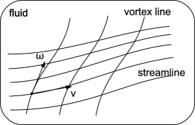
Figure 3.1: Streamlines are lines within the fluid which are tangent, at each point, to velocity vector field $\mathbb{v}$. Vortex lines realize the same idea with the replacement of velocity field by vorticity vector field $\boldsymbol{\omega}$.

So we see that we can also express Eq. (3.1.8) as

$$\boxed{i_{\gamma^{\prime}}d\tilde{v}=0}\hskip 28.45274pt\text{{\color[rgb]{1,0,0}\emph{vortex lines equation}}}$$ (3.1.13)

The exterior derivative of the velocity 1-form $\tilde{v}$, i.e. the 2-form $d\tilde{v}$ introduced in (3.1.11), is called vorticity $2$-form. We see from Eq. (3.1.13) that, geometrically speaking, vortex lines direction is the direction which annihilates the vorticity $2$-form.

[The concept of a vortex line is not to be confused with a different concept of line vortex. The latter denotes the situation (particular flow) when the magnitude of vorticity vector is negligible outside a small vicinity of a line (tornado providing a well-known example). So, in the case of line vortex, there is a single particular line within the fluid volume (defined as the line where vorticity is sufficiently large) whereas, usually, there is a lot of vortex lines, one passing through each point of the volume.]

3.1.3 Acceleration term reexpressed

In Eq. (3.1.6) two vector fields are equated. One can easily express the same content by equating two covector fields (i.e. 1-forms; forms turn out to be fairly convenient for treating vortices, as we already mentioned in the last paragraph).

On the l.h.s. of Eq. (3.1.6), notice that the (standard = Riemann/Levi-Civita) covariant derivative commutes with raising and lowering of indices (since the connection is metric). Therefore

$$\tilde{a}\equiv g(a,\ .\ )\equiv g(\nabla_{v}v,\ .\ )=\nabla_{v}(g(v,\ .\ ))\equiv\nabla_{v}\tilde{v}$$ (3.1.14)

On the r.h.s. of Eq. (3.1.6), the relation between gradient as a vector field and gradient as a covector field may be used:

$$g(\text{\rm grad\,}f,\ .\ ):=df\hskip 28.45274pt\text{i.e.}\hskip 28.45274pt(\text{\rm grad\,}f)^{i}=g^{ij}(df)_{j}\equiv g^{ij}\partial_{j}f$$ (3.1.15)

Putting all this together we get

$$\nabla_{v}\tilde{v}=-\frac{1}{\rho}\ dp-d\Phi$$ (3.1.16)

Now, we can reexpress the covariant derivative in terms of Lie derivative and, finally, in terms of the exterior and interior derivatives:

$$\nabla_{v}\tilde{v} = \mathcal{L}_{v}\tilde{v}-(\nabla v)(\tilde{v})$$ (3.1.17)

$$= i_{v}d\tilde{v}+d(v^{2}/2)\hskip 28.45274ptv^{2}\equiv g(v,v)$$ (3.1.18)

$\blacktriangledown\hskip 14.22636pt$ A proof: First, in general we have

$$\begin{array}[]{rcl}\mathcal{L}_{W}\langle\alpha,V\rangle&=&\nabla_{W}\langle\alpha,V\rangle\\ \langle\mathcal{L}_{W}\alpha,V\rangle+\langle\alpha,\mathcal{L}_{W}V\rangle&=&\langle\nabla_{W}\alpha,V\rangle+\langle\alpha,\nabla_{W}V\rangle\\ \langle\mathcal{L}_{W}\alpha,V\rangle+\langle\alpha,[W,V]\rangle&=&\langle\nabla_{W}\alpha,V\rangle+\langle\alpha,\nabla_{V}W+[W,V]\rangle\\ \langle\mathcal{L}_{W}\alpha,V\rangle&=&\langle\nabla_{W}\alpha,V\rangle+(\nabla W)(V,\alpha)\\ \mathcal{L}_{W}\alpha&=&\nabla_{W}\alpha+(\nabla W)(\alpha)\end{array}$$

Here, $\nabla W$ is a tensor of type $\binom{1}{1}$ and $(\nabla W)(\alpha)$ looks in components

$$((\nabla W)(\alpha))_{i}=(\nabla W)_{i}^{j}\alpha_{j}=W^{j}_{\ ;i}\alpha_{j}$$

Now, in our particular case in Cartesian coordinates, where $i)$ all $\Gamma$’s vanish and $ii)$ $v^{j}=v_{j}$, we have

$$((\nabla v)(\tilde{v}))_{i}=v^{j}_{\ ;i}v_{j}=v_{j,i}v_{j}=(v_{j}v_{j}/2)_{,i}=(dv^{2}/2)_{i}$$

This is, however, tensorial equation (i.e. independent of coordinates), so

$$\nabla_{v}\tilde{v}=\mathcal{L}_{v}\tilde{v}-d(v^{2}/2)$$

Finally, due to Cartan’s identity $\mathcal{L}_{v}=i_{v}d+di_{v}$, we see that Eq. (3.1.18) holds. $\blacktriangle$

Plugging Eq. (3.1.18) into Eq. (3.1.16) we get

$$i_{v}d\tilde{v}=-\frac{1}{\rho}\ dp-d(\Phi+v^{2}/2)$$ (3.1.19)

This can be, of course, expressed back in the language of standard vector analysis. Using formulas collected in Appendix A, we get

$$\mathbb{v}\times(\boldsymbol{\nabla}\times\mathbb{v})=\frac{1}{\rho}\ \boldsymbol{\nabla}p+\boldsymbol{\nabla}(\Phi+v^{2}/2)$$ (3.1.20)

3.1.4 Conservation of mass and entropy

Let $\Omega$ be the standard volume form and $D\subset M$. Consider the following three integrals:

$$\text{vol}\ D := \int_{D}\Omega\hskip 42.67912pt\text{\emph{volume of $D$}}$$ (3.1.21)

$$m(D) := \int_{D}\rho\Omega\hskip 38.41139pt\text{\emph{total mass in $D$}}$$ (3.1.22)

$$S(D) := \int_{D}s\rho\Omega\hskip 34.14322pt\text{\emph{total entropy in $D$}}$$ (3.1.23)

[One could wonder why the product $s\rho$, and not just $s$, enters the expression in Eq. (3.1.23) of total entropy in domain $D\subset M\equiv E^{3}$. The reason is that $s$ denotes entropy per unit mass. So, by definition, $s\delta m$ is entropy of infinitesimal mass $\delta m$ of the fluid. Since $\delta m=\rho\delta V$ (i.e. $\rho$ denotes mass per unit volume), the amount $\delta S$ of entropy in volume $\delta V$ is $\delta S=s\delta m=s\rho\delta V$.]

The total mass of the fluid in $D$, Eq. (3.1.22), is conserved. Simply $m(D(t))$ is the same amount of mass as $m(D(0))$, it just traveled (formally via the flow $\Phi_{t}$ generated by $v$) to some other place.

The total entropy of the fluid in $D$, Eq. (3.1.23), is conserved as well. This is because of the fact, that the fluid is ideal. There is no heat exchange between different parts of the fluid, no energy dissipation caused by internal friction, viscosity, in the fluid. So the motion of ideal fluid is to be treated as adiabatic. Entropy $S(D(t))$ is the same as $S(D(0))$.

We can also express the two facts differently:

both $$m(D) S(D)$$ and are absolute integral invariants.

Such a situation was already discussed in detail in general context of integral invariants in Section 2.6. So here, first, we have as many as two continuity equations à la Eq. (2.6.8), playing role of differential versions of Eqs. (3.1.22) and (3.1.23):

$$\boxed{{\text{\rm div\,}}(\rho v)=0}\hskip 31.2982pt\text{(\emph{continuity equation for mass})}$$ (3.1.24)

$$\boxed{{\text{\rm div\,}}(s\rho v)=0}\hskip 28.45274pt\text{(\emph{continuity equation for entropy})}$$ (3.1.25)

This just corresponds to the existence of two “isolated” integral invariants.

But the two integral invariants are actually related in a specific way described in Sec. 2.6, see Eq. (2.6.16) and below. Notice, however, that the correspondence is a bit tricky:

$$\Omega\ ,\ \rho\Omega \leftrightarrow \rho\Omega\ ,\ s(\rho\Omega)$$   there                       here

From this fact we can deduce, according to (time-independent version of) Eq. (2.6.18), that

$$\boxed{vs=0}$$ (3.1.26)

This says that $s$ is constant along streamlines (integral lines of the velocity field $v$). The constant may, in general, take different values on different streamlines.

$\blacktriangledown\hskip 14.22636pt$ A direct proof: Eq. (3.1.25) says

$${\text{\rm div\,}}(s\rho v)=\rho(vs)+s{\text{\rm div\,}}(\rho v)=0$$

Then Eq. (3.1.24) leads to Eq. (3.1.26). We used ${\text{\rm div\,}}(fu)=uf+f{\text{\rm div\,}}u$, which follows from

$$0=i_{u}(df\wedge\Omega)=(uf)\Omega-df\wedge i_{u}\Omega$$

and

$$\begin{array}[]{rcl}0&=&{\text{\rm div\,}}(fu)\Omega\\ &=&(di_{fu}+i_{fu}d)\Omega\\ &=&d(fi_{u}\Omega)\\ &=&df\wedge i_{u}\Omega+(f{\text{\rm div\,}}u)\Omega\\ &=&(uf+f{\text{\rm div\,}}u)\Omega\end{array}$$

$\blacktriangle$

3.1.5 Barotropic fluid

In general, equation of state of the fluid may be written as $p=p(V,s)$, where $s$ is (specific) entropy (i.e. entropy per unit mass) and $V$ is (specific) volume (i.e. volume per unit mass). Or, alternatively, as

$$p=p(\rho,s)\hskip 28.45274pt\text{general fluid}$$ (3.1.27)

since $\rho=1/V$. In this case, Eq. (3.1.19) is the final form of Euler equation for stationary flow.

However, one can think of an important model, when the pressure depends on $\rho$ alone:

$$p=p(\rho)\hskip 36.98866pt\text{\emph{barotropic} fluid}$$ (3.1.28)

(In particular, we speak of polytropic case, if $p=K\rho^{\gamma}$, $K=$ const.). It is a useful model for fluid behavior in a wide variety of situations. Then, clearly

$$d\left(\frac{1}{\rho}\ dp\right)=0$$ (3.1.29)

So, there is a function, $P$, such that

$$\frac{1}{\rho}\ dp=dP$$ (3.1.30)

In order to interpret $P$ physically, consider the general thermodynamic relation

$$dw=Tds+Vdp\equiv Tds+\frac{1}{\rho}\ dp$$ (3.1.31)

where $w$ is enthalpy (heat function) per unit mass. So $dp/\rho$ is not exact, in general. From Eq. (3.1.26) we see that $ds(v)=0$, This means that, at each point of the fluid, the 1-form $ds$ vanishes when restricted onto a particular 1-dimensional subspace (spanned by $v$) but it, in general, does not vanish as a 1-form, i.e. on arbitrary vector at that point. (There are good reasons, mentioned above, for $s$ to be constant along a single streamline, however, there is no convincing reason for the constant to have the same value on neighboring streamlines.)

So, if we search for a situation, when $dp/\rho$ is exact (i.e. Eq. (3.1.30) holds) we have to have, according to Eq. (3.1.31), $ds=0$ as a 1-form (on any argument, no just on $v$). This means, however

$$s=\ \text{const.}$$ (3.1.32)

throughout the volume of the fluid, not just along streamlines (or, put it differently, the constants the function $s$ takes on different streamlines should be equal, now). So, barotropic case is the one when Eq. (3.1.26) is fulfilled “trivially” as Eq. (3.1.32). Although it may seem to be a rare situation, one can read in $2 of [Landau, Lifshitz 1987] that, on the contrary, “it usually happens” (barotropic is called isentropic, there). Denoting $w=P$, we get (3.1.30).

3.1.6 Final form of stationary Euler equation

Using Eq. (3.1.30) in Eq. (3.1.19), we get our final form of the equation of motion governing stationary and barotropic flow of ideal fluid:

$$\boxed{i_{v}d\tilde{v}=-d\mathcal{E}}\hskip 28.45274pt\text{{\color[rgb]{1,0,0}\emph{Euler equation}}}\hskip 14.22636pt(\text{{\color[rgb]{1,0,0}\emph{stationary}, \emph{barotropic}}})$$ (3.1.33)

Here

$$\boxed{\mathcal{E}:=v^{2}/2+P+\Phi}\hskip 28.45274pt\text{\emph{Bernoulli function}}$$ (3.1.34)

Remember, however, that for more general, non-barotropic flow we have to use more general equation (3.1.19). In what follows we mainly concentrate on Eq. (3.1.33).

Equation (3.1.33) can also be expressed in terms of good old vector analysis. Using formulas collected in Appendix A, we get (see Eq. (3.1.20))

$$\mathbb{v}\times(\boldsymbol{\nabla}\times\mathbb{v})=\boldsymbol{\nabla}\mathcal{E}$$ (3.1.35)

3.2 Simple consequences of stationary Euler equation

3.2.1 Fluid statics (hydrostatics)

Statics means that fluid does not flow at all, i.e. $v=0$. (So what still remains unknown is $p$ and $\rho$ as functions of $\mathbb{r}$.)

Plugging this into Eqs. (3.1.33) and (3.1.34) we get

$$dP+d\Phi=0$$ (3.2.1)

Or, more generally (relaxing barotropic assumption, see Eq. (3.1.30)),

$$\boxed{\frac{dp}{\rho}+\ d\Phi=0}\hskip 28.45274pt\text{{\color[rgb]{1,0,0}\emph{fluid statics equation}}}\hskip 8.5359pt\text{(\emph{hydrostatic equilibrium})}$$ (3.2.2)

Example 3.2.1.1: Water in a swimming pool.

Water is incompressible, so $\rho=\rho_{0}=$ const. (So the only unknown quantity is $p(\mathbb{r})$.) For gravitational field we have $\Phi(x,y,z)=gz$. Therefore

$$dp=-\rho_{0}gdz=d(-\rho_{0}gz)$$ (3.2.3)

and

$$p(x,y,z)=p_{0}-\rho_{0}gz$$ (3.2.4)

So the pressure linearly increases with depth in water. The end of Example 3.2.1.1.

Example 3.2.1.2: Polytropic atmosphere.

The atmosphere (air) is compressible, so both $p$ and $\rho$ are unknown. Since we are still in gravitational field, $\Phi(x,y,z)=gz$ again. From symmetry we can assume both quantities depend on $z$ alone, $p(z)$ and $\rho(z)$.

The main assumption is that

$$p(\rho)=K\rho^{\gamma}\hskip 28.45274pt\text{\emph{polytropic fluid}}\hskip 28.45274ptK,\gamma=\ \text{const.}$$ (3.2.5)

(This is a particular instance of barotropic assumption $p=p(\rho)$ from Eq. (3.1.28).)

Let us start with isothermal case, i.e. $\gamma=1$.

[Equation of state for $\nu$ moles of ideal gas is

$$pV=\nu RT\hskip 28.45274pt\text{i.e.}\hskip 28.45274ptp=p(\rho,T)=\frac{RT}{M_{1}}\ \rho$$ (3.2.6)

where $V=\nu V_{1}$ is volume of $\nu$ moles and $M=\rho V=\rho\nu V_{1}=\nu M_{1}$ is mass of $\nu$ moles. For $T=T_{0}=$ const. we get Eq. (3.2.5) for $K=RT_{0}/M_{1}$ and $\gamma=1$.]

Then Eq. (3.2.2) says

$$\frac{d\rho}{\rho}=-\left(\frac{M_{1}g}{RT_{0}}\right)dz\equiv-\frac{dz}{z_{0}}\hskip 28.45274pt\rho=\rho(z)$$ (3.2.7)

where the isothermal scale-height of the atmosphere is

$$z_{0}:=\frac{RT_{0}}{M_{1}g}=\frac{kT_{0}}{m_{1}g}$$ (3.2.8)

[Recall that $R=N_{A}k$, where $N_{A}$ is Avogadro number (number of constituent particles, usually atoms or molecules, per mole) and $k$ is Boltzmann constant. Moreover, $M_{1}=N_{A}m_{1}$, where $m_{1}$ is mass of a single particle. So $z_{0}=(N_{A}kT_{0})/(N_{A}m_{1}g)$, or

$$m_{1}gz_{0}=kT_{0}$$ (3.2.9)

Therefore $z_{0}$ is the height in which gravitational potential energy of the particle equals energy $kT_{0}$.]

From Eqs. (3.2.7) and (3.2.6) we get that both mass density and pressure decrease exponentially with altitude

$$\rho(z) = \rho_{0}e^{-z/z_{0}}$$ (3.2.10)

$$p(z) = p_{0}e^{-z/z_{0}}$$ (3.2.11)

where $p_{0}=p(0)$, $\rho_{0}=\rho(0)$. Notice that

$$e^{-z/z_{0}}=e^{-m_{1}gz/kT_{0}}$$ (3.2.12)

is nothing but the Boltzmann factor $e^{-U/kT}$.

Adiabatic case corresponds to $1\neq\gamma=c_{p}/c_{V}$ and $K=p_{0}/\rho_{0}^{\gamma}$ in the polytropic formula Eq. (3.2.5). We get, instead of Eq. (3.2.7),

$$K^{1/\gamma}p^{-1/\gamma}dp=-gdz\hskip 25.6073pt\text{i.e.}\hskip 25.6073ptd\left(\frac{K^{1-\Gamma}}{\Gamma}p^{\Gamma}\right)=d(-gz)$$ (3.2.13)

where $\Gamma\equiv 1-1/\gamma$. This results in

$$\rho(z) = \rho_{0}\left(1-\frac{\gamma-1}{\gamma}\frac{z}{z_{0}}\right)^{\frac{1}{\gamma-1}}$$ (3.2.14)

$$p(z) = p_{0}\left(1-\frac{\gamma-1}{\gamma}\frac{z}{z_{0}}\right)^{\frac{\gamma}{\gamma-1}}$$ (3.2.15)

$$T(z) = T_{0}\left(1-\frac{\gamma-1}{\gamma}\frac{z}{z_{0}}\right)$$ (3.2.16)

[For adiabatic case $pV^{\gamma}=p_{0}V_{0}^{\gamma}$ with $\gamma=c_{p}/c_{V}$. With the help of $\rho V=\nu M_{1}$ this can be rewritten as $p/\rho^{\gamma}=p_{0}/\rho_{0}^{\gamma}$, or $p=(p_{0}/\rho_{0}^{\gamma})\rho^{\gamma}$, so that $p=K\rho^{\gamma}$ with $K=p_{0}/\rho_{0}^{\gamma}$. Integration of Eq. (3.2.13) gives Eq. (3.2.15), $p=K\rho^{\gamma}$ leads to Eq. (3.2.14) and finally equation of state Eq. (3.2.6) provides us with Eq. (3.2.16).]

As we see from Eq. (3.2.16), the temperature of the atmosphere falls off linearly with increasing height above ground level.

Also notice that for $\gamma\to 1$ we return to isothermal case treated before, i.e. we get $T(z)=T_{0}$ and exponential decrease of mass density and pressure given by Eqs. (3.2.10) and (3.2.11). The end of Example 3.2.1.2.

3.2.2 Bernoulli equation

Let us apply $i_{v}$ on both sides of Eq. (3.1.33). We get

$$\boxed{v\mathcal{E}=0}\hskip 28.45274pt\text{{\color[rgb]{1,0,0}\emph{Bernoulli equation}}}$$ (3.2.17)

(D.Bernoulli 1738). This says that $\mathcal{E}$ is constant along streamlines (integral lines of the velocity field $v$). The constant may take different values on different streamlines (see Fig. 3.2).

For incompressible fluid (i.e. when $\rho=\rho_{0}=$ const., e.g. for water) in gravitational field (i.e. when $\Phi(\mathbb{r})=gz$), equation (3.2.17) takes its more familiar form

$$\rho_{0}v^{2}/2+p+\rho_{0}gz=\ \text{const.}$$ (3.2.18)

Another way to regard Eq. (3.2.17) comes from comparison with the statement $vs=0$, Eq. (3.1.26). We know that the latter is just differential way to express the fact that entropy is conserved in the sense that Eq. (3.1.23) is absolute integral invariant. So, Bernoulli equation also says that “moving particle” (in hydrodynamic terminology, a fixed small amount of mass of the fluid; equivalent expressions are “fluid particle”, “fluid element”, “fluid parcel” or “material element”) carries with it a constant value of $\mathcal{E}$.

Figure 3.2: Left: according to Bernoulli theorem Eq. (3.2.17), the function $\mathcal{E}$ is constant on any streamline. However, the constant may take different values on different streamlines. Right: if the flow is vorticity-free, the constant is the same even on different streamlines, see Eq. (3.2.19).

Now, consider a stationary, barotropic and, in addition, vorticity-free flow. In this particular case, the vorticity 2-form vanishes in Eq. (3.1.33), $d\tilde{v}=0$ (cf. (3.1.7) and (3.1.11)). We get $d\mathcal{E}=0$, or, consequently

$$\boxed{\mathcal{E}=\ \text{const.}}$$ (3.2.19)

So, $\mathcal{E}$ is constant along streamlines irrespective of whether vorticity vanishes or not (stationary and barotropic flow is enough), but in order that $\mathcal{E}$ is constant in the bulk of the fluid, the flow is to be vorticity-free.

3.2.3 Kelvin’s theorem on circulation - stationary case

Let us display, side by side in one line, Eq. (3.1.33) versus Eq. (2.2.12), i.e. the stationary Euler equation versus the core equation of the general theory of Poincaré version of integral invariants:

$$i_{v}(d\tilde{v})=-d\mathcal{E}\hskip 28.45274pt\leftrightarrow\hskip 28.45274pti_{v}(d\alpha)=d\beta$$ (3.2.20)

We see that stationary Euler equation may be regarded as a particular example of the equation which is central in general scheme of integral invariants, provided that we make the identification

$$\alpha\leftrightarrow\tilde{v}\hskip 28.45274pt\beta\leftrightarrow-\mathcal{E}\hskip 28.45274ptv\leftrightarrow v$$ (3.2.21)

Then, however, all consequences are (almost) automatic. Here we simply rewrite the general result on relative integral invariant (2.2.14) using the vocabulary from Eq. (3.2.21) and obtain

$$\boxed{i_{v}d\tilde{v}=-d\mathcal{E}\hskip 14.22636pt\Rightarrow\hskip 14.22636pt\oint_{c}\tilde{v}=\ \ \text{\emph{relative} invariant}}$$ (3.2.22)

[Notice the implication sign here where equivalence sign is present in Eq. (2.2.14). The reason is actually explained, in general context, in the note following Eq. (2.2.14). Here, the fact that the integral on the r.h.s. of Eq. (3.2.22) behaves invariantly would be true for any function $\mathcal{E}$ in $i_{v}d\tilde{v}=-d\mathcal{E}$. In Euler equation, however, $\mathcal{E}$ is a concrete function, namely $\mathcal{E}:=v^{2}/2+P+\Phi$, see Eq. (3.1.34). Clearly, this particular $\mathcal{E}$ cannot be deduced from the invariance property of the integral.]

In traditional notation (see (3.1.10)), the integral in Eq. (3.2.22) is called

$$\oint_{c}\tilde{v}\equiv\oint_{c}\mathbb{v}\cdot d\mathbb{r}\hskip 42.67912pt\text{\emph{velocity circulation}}$$ (3.2.23)

and the statement is that it represents a relative integral invariant

$$\boxed{\oint_{c}\mathbb{v}\cdot d\mathbb{r}=\text{const.}}\hskip 42.67912pt\text{{\color[rgb]{1,0,0}\emph{Kelvin's theorem}} }$$ (3.2.24)

([Kelvin 1869]; see e.g. $8 in [Landau, Lifshitz 1987], $1.2 in [Chorin, Marsden 1993] or $5.3 in [Batchelor 2002]). In words: in an ideal fluid, the velocity circulation round a closed fluid contour is constant in time. (Here “fluid contour” is a closed path moving together with the fluid. That is, a contour moving by the flow $c\mapsto\Phi_{t}(c)$, where $\Phi_{t}\leftrightarrow v$.)

[Notice that $c$ in Eq. (3.2.24) is a general 1-cycle (loop). That is, not necesarilly a boundary of a 2-chain (i.e. of 2-dimensional surface). (So $\partial c=0$ is compulsory, $c=\partial S$ is not.) As an example, it may be a tangly knot.]

By applying the simple general rule (2.2.16) we also get an absolute invariant given as a surface integral of the corresponding two-form:

$$\int_{S}d\tilde{v}=\ \ \text{\emph{absolute} invariant}$$ (3.2.25)

In traditional notation (see (3.1.11)), the integral in Eq. (3.2.25) is called

$$\int_{S}d\tilde{v}\equiv\int_{S}(\text{\rm curl\,}\mathbb{v})\cdot d\mathbb{S}\equiv\int_{S}\boldsymbol{\omega}\cdot d\mathbb{S}\hskip 42.67912pt\text{\emph{vorticity flux}}$$ (3.2.26)

and the statement is that it represents an absolute integral invariant

$$\boxed{\int_{S}\boldsymbol{\omega}\cdot d\mathbb{S}=\text{const.}}$$ (3.2.27)

In words: in an ideal fluid, the vorticity flux through fluid surface is constant in time. (Here “fluid surface” is a surface moving together with the fluid. That is, a surface moving by the flow $S\mapsto\Phi_{t}(S)$, where $\Phi_{t}\leftrightarrow v$.)

[Let $\boldsymbol{\omega}$ be, at some fixed time $t$, (non-vanishing) vorticity vector in a given point $P$ of the fluid. At this point consider surface elements $d\mathbb{S}=\mathbb{n}dS$ with fixed $dS$ and all possible directions $\mathbb{n}$. Then clearly $\boldsymbol{\omega}\cdot d\mathbb{S}$ is maximum for $d\mathbb{S}$ directed along $\boldsymbol{\omega}$. Due to Stokes theorem, however, $\boldsymbol{\omega}\cdot d\mathbb{S}$ is integral of $\mathbb{v}$ around the boundary of the (infinitesimal) surface $d\mathbb{S}$, i.e. the velocity circulation round the boundary of $d\mathbb{S}$. So, the direction of the vorticity vector $\boldsymbol{\omega}$ is the direction of maximum velocity circulation. Therefore, going along a vortex line is actually going, in each point of the line, in the direction with maximum velocity circulation round a small circle drawn in the plane perpendicular to the direction. Naively, this is then the direction about which, at the point $P$ at time $t$, the fluid particle rotates (in addition to its translational motion).]

3.2.4 Helmholtz theorem on vortex lines - stationary case

In order to obtain Bernoulli equation (3.2.17) we just applied the interior derivative $i_{v}$ on both sides of Euler equation (3.1.33).

Another obvious thing to do with Euler equation (3.1.33) to get something interesting is to apply the exterior derivative $d$ on both sides. What we obtain now is

$$\mathcal{L}_{v}(d\tilde{v})=0$$ (3.2.28)

This is, however, nothing but infinitesimal version of the statement

$$\Phi_{t}^{*}(d\tilde{v})=d\tilde{v}\hskip 56.9055pt\Phi_{t}\leftrightarrow v$$ (3.2.29)

So the vorticity 2-form $d\tilde{v}$ is invariant w.r.t. the flow $\Phi_{t}$ generated by $v$, i.e. w.r.t. “real flow” of the fluid.

Consider, at time $t_{0}$, an arbitrarily parametrized vortex line $\gamma(\lambda)$. (So it is, actually, a “vortex curve”; the parametrization is, however, arbitrary). Due to the flow $\Phi_{t}$, its point $\gamma(\lambda)$ moves along the streamline (integral curve) of $v$ and, at time $t_{0}+t$, it is at the point

$$\Phi_{t}(\gamma(\lambda))\equiv(\Phi_{t}\circ\gamma)(\lambda)=:\gamma_{t}(\lambda)$$ (3.2.30)

Since this happens with each point of the original vortex line $\gamma$, the line itself moves, within the time interval from $t_{0}$ to $t_{0}+t$, to a new line, $\gamma_{t}$. And it is not clear at all, apriori, whether or not the new line, $\gamma_{t}$, is a vortex line, too.

More than one and a half century ago (in 1858), Helmholtz gave positive answer to the question ([Helmholtz 1858]):

$$\{\gamma=\text{vortex line}\}\hskip 14.22636pt\Rightarrow\hskip 14.22636pt\{\gamma_{t}=\text{vortex line}\}\hskip 14.22636pt\text{{\color[rgb]{1,0,0}\emph{Helmholtz theorem}}}$$ (3.2.31)

His theorem asserts that, under the flow of ideal barotropic fluid, vortex lines always move to vortex lines again. It is often expressed by saying that vortex lines are “frozen” into a perfectly inviscid (= ideal) barotropic fluid (in the sense that they “move with the fluid”) or that they “move as material lines”.

Figure 3.3: Helmholtz theorem Eq. (3.2.31) says that, under the flow of ideal barotropic fluid, vortex lines always move to vortex lines again (so vortex lines are “frozen” into the fluid).

[It turns out that the physics behind the theorem is closely related to the ubiquitous angular momentum conservation. The angular momentum of the fluid in a small piece of a vortex tube cannot change, since the fluid is ideal (i.e. inviscous) and therefore there are no tangential forces on the surface of the piece of the tube. See a nice exposition in Sec. 40-5 of [Feynman 1964].

On the other hand, one is to proceed with due caution, as we can read in Sec. 5.3 of [Batchelor 2002]:

“There is an obvious temptation to interpret some of these results as a consequence of conservation of angular momentum of the fluid contained in the vortex-tube. Such an interpretation is possible when the cross-section of the vortex-tube is small and circular, and remains circular, since the (inviscid) stress at the boundary of the vortex-tube then exerts no couple on the fluid in the vortex-tube. In more general circumstances the strength of a vortex- tube is not simply proportional to the angular momentum of the fluid in unit length of the tube, and more is involved in the above results than a simple conservation of angular momentum.”]

Let’s see how (easily) this follows from Eq. (3.2.29). At time $t_{0}$, the tangent vector $\gamma^{\prime}$ to the original “vortex curve” $\gamma(\lambda)$ annihilates, according to Eq. (3.1.13), the vorticity $2$-form $d\tilde{v}$. At time $t_{0}+t$, the curve becomes $(\Phi_{t}\circ\gamma)(\lambda)$. Its tangent vector, therefore, becomes $\Phi_{t*}\gamma^{\prime}$ (it follows from the definition of push-forward operation). So, the issue is whether

$$i_{\gamma^{\prime}}d\tilde{v}=0\hskip 28.45274pt\Rightarrow\hskip 28.45274pti_{\Phi_{t*}\gamma^{\prime}}d\tilde{v}=0$$ (3.2.32)

holds or, equivalently, whether

$$(d\tilde{v})(\Phi_{t*}\gamma^{\prime},w)=0$$ (3.2.33)

for any $w$ (sitting at the same point as $\Phi_{t*}\gamma^{\prime}$). But any $w$ may be regarded as $\Phi_{t*}u$ for some $u$ (sitting at the same point as $\gamma^{\prime}$; namely $u=\Phi_{-t*}w$). So, we get for the l.h.s. of Eq. (3.2.33)

$$(d\tilde{v})(\Phi_{t*}\gamma^{\prime},\Phi_{t*}u)=(\Phi_{t}^{*}d\tilde{v})(\gamma^{\prime},u)=(d\tilde{v})(\gamma^{\prime},u)=(i_{\gamma^{\prime}}d\tilde{v})(u)=0$$ (3.2.34)

Therefore, because of invariance of $d\tilde{v}$ w.r.t. the flow $\Phi_{t}$, tangent vectors which annihilate the $2$-form at some time flow to tangent vectors which also do annihilate the $2$-form at later times and this means that vortex lines always flow to vortex lines again.

The reader who grasped material discussed in the Chapter 2 (devoted to integral invariants in general) probably noticed that the main statement presented here may be regarded as a particular case of the result presented in Sec. 2.7 (and also the proof is very similar). We return to Helmholtz theorem again in Sec. 3.4.3. There we learn that it holds even for non-stationary flow. (Sec. 2.7 treats non-stationary theory from the very beginning.)

3.2.5 Related Helmholtz theorems - stationary case

In literature one often finds three “classical” Helmholtz theorems closely related to our statement Eq. (3.2.31). They follow easily from what was said before, including Kelvin’s theorem on circulation, Eq. (3.2.24). Recall, however, that the Helmholtz paper was published 11 years sooner than the Kelvin’s one - in 1858 versus 1869, respectively).

Let us first introduce a few new concepts.

Vortex sheet is a (2-dimensional) surface composed from vortex lines (i.e. it is a 1-parameter family of vortex lines, passing through the same curve in space). In particular it reduces to vortex tube if the curve becomes a loop, the boundary of a surface in space (so the vortex tube is a vortex sheet rolled so as to form a tube). And finally, vortex filament is a vortex tube whose “cross-section” is of infinitesimal dimensions. (A common name for all these objects is vortex structures.)

It is obvious that Helmholtz theorem concerning vortex lines, Eq. (3.2.31), immediately leads to corresponding statement concerning vortex tubes (or structures, in general):

Vortex tubes always move to vortex tubes again. (3.2.35)

At time $t=0$, fix a vortex tube. Consider a cross-section $S$ of the tube (2-dimensional surface cutting the tube). Then its boundary, $c=\partial S$, is a loop which encircles the tube once. Stokes theorem says that

$$\int_{S}d\tilde{v}=\int_{c}\tilde{v}$$ (3.2.36)

So, velocity circulation round the boundary $c$ of the cross-section $S$ equals the vorticity flux through $S$ itself.

Now, take another cross-section, $S^{\prime}$, with the same boundary $c$ (so $c=\partial S=\partial S^{\prime}$). Then the two fluxes (through $S$ and $S^{\prime}$, respectively) are equal,

$$\int_{S}d\tilde{v}=\int_{S^{\prime}}d\tilde{v}$$ (3.2.37)

since the r.h.s. of Eq. (3.2.36) does not contain any particular choice of the cross-section, it feels its boundary alone.

What is more interesting, however, is that the flux even does not depend on the choice of the loop $c$ encircling the tube! So, it is a number which characterizes the tube itself:

$$\int_{S}d\tilde{v}\equiv\int_{S}\boldsymbol{\omega}\cdot d\mathbb{S}\hskip 28.45274pt\text{\emph{stregth of the tube}}$$ (3.2.38)

(It is the vorticity flux through any cross-section $S$ cutting the tube.)

$\blacktriangledown\hskip 14.22636pt$ We provide as many as two proofs, since each one might be instructive, albeit from different point of view.

Proof 1.: This is just a version of the “amazingly simple” proof from Eqs. (2.4.8) and (2.4.9): let $c_{1}$ and $c_{2}$ be the boundaries of $S_{1}$ and $S_{2}$ respectively (see Fig. 3.4) and let $\Sigma$ be the (2-dimensional) part of the tube enclosed by $c_{1}$ and $c_{2}$ (so that $\partial\Sigma=c_{1}-c_{2}$). Then

$$\int_{\Sigma}d\tilde{v} \overset{1.}{=} \oint_{\partial\Sigma}\tilde{v}=\oint_{c_{1}}\tilde{v}-\oint_{c_{2}}\tilde{v}=\int_{S_{1}}d\tilde{v}-\int_{S_{2}}d\tilde{v}$$ (3.2.39)

$$\overset{2.}{=} 0$$ (3.2.40)

Figure 3.4: A solid vortex tube $V$ (the tube inside) is made of vortex lines emanating from the left cap $S_{1}$ and entering the right cap $S_{2}$. Boundary $\partial V$ of the solid cylinder $V$ consists of 3 parts, $\partial V=\Sigma+S_{2}-S_{1}$, hollow cylinder $\Sigma$ (“side” of the solid cylinder) and the two caps, $S_{1}$ and $S_{2}$. We have $0=\partial\partial V=\partial\Sigma+\partial S_{2}-\partial S_{1}$, so $\partial\Sigma=\partial S_{1}-\partial S_{2}=c_{1}-c_{2}$. The cycles $c_{1}$ and $c_{2}$ encircle the same tube of vortex lines.

Justification of the second equality (saying that the surface integral actually vanishes) repeats the argument used in the text following Eqs. (2.4.8) and (2.4.9), replacing $\xi$ by $u$ (a vector along the vortex line, i.e. obeying $i_{u}d\tilde{v}=0$).

Proof 2.: Let $u$ be a vector field defined by $i_{u}d\tilde{v}=0$, i.e. a field tangent, at each point, to the vortex line passing through the point; there is a freedom $u\mapsto fu$ in the choice of $u$, $f$ being a function. So, the flow $\Phi_{s}$ of $u$ leaves each vortex line invariant (as a set). Therefore, the same holds for the vortex tube.

Consider the (artificial!) “dynamics” given by $u$. Then the equation $i_{u}d\tilde{v}=0$ may be regarded as a particular case of the basic equation (2.2.14), $i_{v}d\alpha=d\beta$, from the general theory of integral invariants (with $v\mapsto u$, $\alpha\mapsto\tilde{v}$ and $\beta\mapsto 0$; notice that solutions from Sec.2.4 become vortex lines, here, and the tube of solutions becomes the vortex tube). So,

$$\oint_{c}\tilde{v}=\text{relative invariant}$$ (3.2.41)

and, consequently,

$$\int_{S}d\tilde{v}=\text{absolute invariant}$$ (3.2.42)

both of them for our “artificial dynamics” generated by $u$ (as opposed to the real dynamics generated by the fluid velocity field $v$). However, Eq. (3.2.42) exactly says that the vorticity flux does not depend on the particular choice of cross-section $S$ cutting the tube. (Just realize that, starting from a fixed cross-section $S_{1}$, one can produce any other $S_{2}$ by means of the flow $\Phi_{s}$ with appropriate $s$ and $u\sim fu$.) $\blacktriangle$

We can write the proved statement as

$$\boxed{\int_{S}\boldsymbol{\omega}\cdot d\mathbb{S}=\text{const.}}$$ (3.2.43)

which looks exactly as Eq. (3.2.27), although it has completely different meaning, now. While Eq. (3.2.27) says that the integral is constant in time (i.e. when the surface flows away as a “material surface” - it changes according to $S\mapsto\Phi_{t}(S)$, $\Phi_{t}\leftrightarrow v$), Eq. (3.2.43), on the contrary, says that the integral is constant “along the vortex tube” (i.e. when $S$ moves - at fixed time - along the tube, so $S\mapsto\Phi_{s}(S)$, $\Phi_{s}\leftrightarrow u$, $i_{u}d\tilde{v}=0$)). These two meanings of the equally looking formula may also be expressed differentially: the vorticity two form $d\tilde{v}$ is Lie-invariant w.r.t. as many as two vector fields:

$$\mathcal{L}_{v}d\tilde{v} = 0\hskip 28.45274pt\text{invariancy w.r.t. motion \emph{in time}}$$ (3.2.44)

$$\mathcal{L}_{u}d\tilde{v} = 0\hskip 28.45274pt\text{invariancy w.r.t. motion \emph{along vortex tube}}$$ (3.2.45)

$\blacktriangledown\hskip 14.22636pt$ The first one immediately results (see Eq. (3.2.28)) from applying $d$ on $i_{v}d\tilde{v}=-d\mathcal{E}$ (Euler equation), the second one from doing the same on $i_{u}d\tilde{v}=0$ (definition of the field $u$ along vortex lines). $\blacktriangle$

Let us summarize the following properties of vortex tubes, which we already know:

- the strength is intrinsic invariant associated with the tube

- it is constant in time as the tube moves

- the tube moves together with the fluid (it is “frozen” in it)

$\blacktriangledown\hskip 14.22636pt$ The first statement follows immediately from Eq. (3.2.43), the second one from Eq. (3.2.27). The third property expresses the content of Eq. (3.2.31). $\blacktriangle$

[As the fluid (and consequently a vortex tube) moves, it sometimes happens that the cross section of the tube decreases its area. (The tube becomes thinner as time goes on. A possible reason may be stretching of the tube in incompressible fluid - like when water flows down a bathtub drain). Since the strength of the tube is to remain the same, the magnitude of the vorticity (i.e. the length of the vorticity vector) necessarily increases to keep the strength. This very phenomenon occurs in tornado. Stretching of vortex tube caused by updrafts of hot air in the atmosphere can result in dramatic magnitude of vorticity.]

Well, and now let us mention what the three Helmholtz celebrated theorems say:

First theorem: The strength of a vortex filament is constant along its length.

Second theorem: A vortex filament cannot end in a fluid;
                  it must extend to the boundaries of the fluid or form a closed path.

Third theorem: A fluid that is initially irrotational remains irrotational.
                 (In the sense that fluid elements initially free of vorticity
                 remain free of vorticity.)

$\blacktriangledown\hskip 14.22636pt$ The first theorem is nothing but the statement given in Eq. (3.2.43).

The second one is discussed at some length (deservedly) in Appendix B and C.

The third one: consider two points, $P$ and $Q=\Phi_{t}(P)$. If some “fluid element” sits at $P$ at time $t=0$, it is at $Q$ at time $t$. Assume the contrary: let the “fluid element” be “rotational” at $Q$, i.e. vorticity $2$-form $d\tilde{v}$ is non-zero at $Q$ at time $t$. This means that there exists an infinitesimal surface $S$ around $Q$ such that $\int_{S}d\tilde{v}\neq 0$. The surface $S$ is $\Phi_{t}$-image of some $S_{0}$ around $P$ (namely of $S_{0}=\Phi_{-t}S$). Therefore

$$0\neq\int_{S}d\tilde{v}=\int_{\Phi_{t}(S_{0})}d\tilde{v}=\int_{S_{0}}\Phi_{t}^{*}d\tilde{v}=\int_{S_{0}}d\tilde{v}$$

and this means that vorticity $2$-form $d\tilde{v}$ is non-zero at $P$ and, consequently, that the “fluid element” is “rotational” at $P$. $\blacktriangle$

3.2.6 Ertel’s theorem

All the statements of the last three sections (Bernoulli equation in Sec. 3.2.2, Kelvin theorem in Sec. 3.2.3 and Helmholtz theorem in Sec. 3.2.4) rest heavily on barotropic assumption $p=p(\rho)$, see Eq. (3.1.28), added to Euler equation in its more general form Eq. (3.1.19). So they assume that Euler equation has its simpler form $i_{v}d\tilde{v}=-d\mathcal{E}$ (see Eq. (3.1.33)).

Here we mention a weaker statement due to Ertel (1942) which is, however, more general in that it does not assume barotropic regime of the fluid.

Recall that the crucial point of derivation of Helmholtz theorem from Euler equation consisted in application of $d$ on Eq. (3.1.33). Let us mimic the procedure replacing, however, Eq. (3.1.33) by the more general one, Eq. (3.1.19).

We get, instead of Eq. (3.2.28), the following equation:

$$\mathcal{L}_{v}(d\tilde{v})=\frac{d\rho\wedge dp}{\rho^{2}}$$ (3.2.46)

So, the vorticity $2$-form $d\tilde{v}\equiv\boldsymbol{\omega}\cdot d\mathbb{S}$ is no longer invariant w.r.t. the flow $\Phi_{t}\leftrightarrow v$.

[Therefore surface integral of the vorticity $2$-form $d\tilde{v}\equiv\boldsymbol{\omega}\cdot d\mathbb{S}$ is no longer integral invariant. Since the integral may be transformed to velocity circulation round the boundary of the surface, Kelvin’s theorem no longer holds. Looking at Eq. (3.2.28) we see, that neither Helmholtz theorem holds for non-barotropic flow. And, finally, applying $i_{v}$ on Eq. (3.1.19), rather than Eq. (3.1.33), we convince ourselves that Bernoulli equation cease to hold as well.]

There is, however, a braver $3$-form which, in spite of truly hard times in this merciless non-barotropic world still remains to be devoted to the noble idea of the concept of $\Phi_{t}\leftrightarrow v$-invariancy.

In order to find this admirable $3$-form, notice that the equation $vs=0$ (3.1.26), which is always true for ideal fluid (i.e. it does not need the fluid to be barotropic), may be written in a slightly more scientific form as

$$\mathcal{L}_{v}s=0$$ (3.2.47)

Applying $d$ we get

$$\mathcal{L}_{v}ds=0$$ (3.2.48)

This means, however, that

$$\mathcal{L}_{v}(ds\wedge d\tilde{v})=0$$ (3.2.49)

$\blacktriangledown\hskip 14.22636pt$ Indeed, we get, first

$$\mathcal{L}_{v}(ds\wedge d\tilde{v})=(\mathcal{L}_{v}ds)\wedge d\tilde{v}+ds\wedge\frac{d\rho\wedge dp}{\rho^{2}}=\frac{ds\wedge d\rho\wedge dp}{\rho^{2}}$$

But the (general) equation of state Eq. (3.1.27) enables one to write $s=s(\rho,p)$, so that $ds=(\dots)d\rho+(\dots)dp$ and the expression above vanishes. $\blacktriangle$

Therefore

$$\int_{D}ds\wedge d\tilde{v}=\ \ \text{\emph{absolute} integral invariant}$$ (3.2.50)

In traditional notation, the statement in Eq. (3.2.50) is known as

$$\int_{D}ds\wedge d\tilde{v}\equiv\boxed{\int_{D}(\boldsymbol{\omega}\cdot\boldsymbol{\nabla}s)dV=\ \text{const.}}\hskip 28.45274pt\text{{\color[rgb]{1,0,0}\emph{Ertel's theorem}}}$$ (3.2.51)

([Ertel 1942]; see also exposition in $5.18 of [Schutz 1980] or $8 in [Landau, Lifshitz 1987]).

$\blacktriangledown\hskip 14.22636pt$ Using formulas from Appendix A we have

$$\begin{array}[]{rcl}ds\wedge d\tilde{v}&=&(\boldsymbol{\nabla}s\cdot d\mathbb{r})\wedge d(\mathbb{v}\cdot d\mathbb{r})\\ &=&(\boldsymbol{\nabla}s\cdot d\mathbb{r})\wedge(\boldsymbol{\omega}\cdot d\mathbb{S})\\ &=&(\boldsymbol{\omega}\cdot\boldsymbol{\nabla}s)dV\end{array}$$

$\blacktriangle$

There is an alternative way to express the message of Eq. (3.2.51). Notice that each $3$-form na $E^{3}$ is proportional to the volume form $\Omega$ or, also, to the $3$-form $\rho\Omega$. So we can define function $f$ such that

$$ds\wedge d\tilde{v}=:f\rho\Omega$$ (3.2.52)

Explicitly, in vector analysis notation,

$$f=\frac{\boldsymbol{\omega}\cdot\boldsymbol{\nabla}s}{\rho}$$ (3.2.53)

$\blacktriangledown\hskip 14.22636pt$ Indeed,

$$\begin{array}[]{rcl}f\rho dV&=&f\rho\Omega\\ &=&ds\wedge d\tilde{v}\\ &=&(\boldsymbol{\omega}\cdot\boldsymbol{\nabla}s)dV\end{array}$$

so that $f\rho=\boldsymbol{\omega}\cdot\boldsymbol{\nabla}s$ as claimed. $\blacktriangle$

From the invariance of the l.h.s. of Eq. (3.2.52), see Eq. (3.2.49), we can immediately infer that

$$\boxed{vf=0}$$ (3.2.54)

This says that, in addition to the function $s$, see Eq. (3.1.26), also the new function $f$ is constant along streamlines (integral lines of the velocity field $v$). The constant may take different values on different streamlines.

[Here we see why exactly the choice of $\rho\Omega$ in the definition of function $f$ in Eq. (3.2.52) is much better than to use just $\Omega$. Namely the proportionality coefficient (function) is only $\mathcal{L}_{v}$-invariant (i.e. Eq. (3.2.54) holds) if it “stands between” two differential forms which are $\mathcal{L}_{v}$-invariant themselves.

Since $\mathcal{L}_{v}(\rho\Omega)=0$ (i.e. mass is conserved) whereas $\mathcal{L}_{v}\Omega\neq 0$ (i.e. volume is not conserved), the right choice is $\rho\Omega$.]

So, for the most general flow of ideal fluid we encountered as many as three absolute integral invariants, all of them based on 3-forms (i.e. given by volume integrals):

$$\int_{D}\rho\Omega\hskip 28.45274pt\int_{D}s\rho\Omega\hskip 28.45274pt\int_{D}f\rho\Omega$$ (3.2.55)

The same objects, when written using notation more frequent in fluid dynamics:

$$\int_{D}dm\hskip 28.45274pt\int_{D}sdm\hskip 28.45274pt\int_{D}fdm$$ (3.2.56)

In words: by any “moving particle” (in hydrodynamic terminology, a fixed small amount of mass of the fluid) constant values of as many as three quantities are carried: $\delta m$ (its mass), $s\delta m$ (its entropy) and $f\delta m$ (the new vorticity-based quantity introduced by Ertel).

What happens with the three integral invariants if we return back to the more specific, barotropic situation? Since $s=$ const. (in the sense of Eq. (3.1.32), not just along $v$), we deduce that

- the second integral is just a constant multiple of the first one

- the constancy of the third integral is the statement $0=$ const.

(The 1-form $ds$ vanishes and both Eqs. (3.2.51) and (3.2.54) become vacuous. Well, the statement $0=$ const. is true, we have to admit, but it seldom helps very much.)

On the other hand, do not forget about Bernoulli equation $v\mathcal{E}=0$ (3.2.17), which also may be regarded in terms of $\mathcal{E}\delta m$ carried by a “moving particle” (as we discussed earlier in Sec. 3.2.2). So, in the barotropic case, we can safely state that we have two non-trivial absolute integral invariants:

$$\int_{D}\rho\Omega\hskip 28.45274pt\int_{D}\mathcal{E}\rho\Omega$$ (3.2.57)

or, in the more usual notation,

$$\int_{D}dm\hskip 28.45274pt\int_{D}\mathcal{E}dm$$ (3.2.58)

3.3 Non-stationary flow

In this section we learn how the general scheme of integral invariants, studied in some detail in Sec. 2, directly offers to express Euler non-stationary equations in a remarkable form from which, among other things, Helmholtz vortex-lines statement results as easily as it was demonstrated, for stationary case, in Section 3.2.4.

3.3.1 Euler equation again - stationary case

Recall that already in Eq. (3.2.20) we displayed, side by side in one line, the stationary Euler equation versus the core equation of the general theory of Poincaré version of integral invariants

$$i_{v}(d\tilde{v})=-d\mathcal{E}\hskip 28.45274pt\leftrightarrow\hskip 28.45274pti_{v}(d\alpha)=d\beta$$ (3.3.1)

This resulted in the following identification of key objects of the two theories

$$\alpha\leftrightarrow\tilde{v}\hskip 28.45274pt\beta\leftrightarrow-\mathcal{E}\hskip 28.45274ptv\leftrightarrow v$$ (3.3.2)

and led to understanding of the Euler stationary equation from Poincaré perspective.

Now the goal is to retell the same physics à la Cartan (i.e. with no change of the content, yet). It is easy, since we know the general algorithm:

First, in the spirit of Eqs. (2.4.1) - (2.4.2), we introduce the $1$-form

$$\sigma:=\tilde{v}-\mathcal{E}dt$$ (3.3.3)

(here, both objects only depend on $\mathbb{r}$, they are stationary) and the vector field

$$\xi:=\partial_{t}+v$$ (3.3.4)

(the field $v$ only depends on $\mathbb{r}$ as well, it is stationary, too). Then, due to Eq. (2.4.4), the stationary Euler equation (3.1.33) is equivalent to

$$i_{\xi}d\sigma=0$$ (3.3.5)

It is that simple.

3.3.2 Euler equation again - non-stationary case

Now we switch to non-stationary case. This is also pretty straightforward, we just follow the logic of general Eqs. (2.5.5) and (2.5.6)). So, the idea is that the value above all is to keep valid the structure of Eq. (3.3.5) even for non-stationary case, i.e. when objects, from which $\sigma$ and $\xi$ are composed, do depend on time (in addition, of course, to their dependence on $\mathbb{r}$):

$$\sigma:=\hat{v}-\mathcal{E}dt$$ (3.3.6)

$$\xi:=\partial_{t}+v$$ (3.3.7)

where, now,

$$v=v(\mathbb{r},t)\hskip 28.45274pt\hat{v}=\hat{v}(\mathbb{r},t)\hskip 28.45274pt\mathcal{E}=\mathcal{E}(\mathbb{r},t)$$ (3.3.8)

[Notation of the (field of the) $1$-form $\tilde{v}$ was changed, in the process of switching from space to space-time, namely from $\tilde{v}$ to $\hat{v}$ (in order to make it clear that we speak of a spatial $1$-form); notation of the fields $v$ and $\mathcal{E}$ remains unchanged, one has to keep in mind, however, that $v$ is a spatial vector field (its time component vanishes) and that, of course, all three objects live in space-time, i.e. they do depend on $t$ as well.]

And what about the ,,decomposed” version of the equation (3.3.5)? We already know the answer in general - it is given in Eq. (2.5.5). So, using the identification of $\hat{\alpha}$ and $\hat{\beta}$ according to (3.3.6) and (3.3.7), we get

$${\mathcal{L}}_{\partial_{t}}\hat{v}+i_{v}\hat{d}\hat{v}=-\hat{d}\mathcal{E}$$ (3.3.9)

Therefore, (non-stationary, but still barotropic) Euler equation may be written in any of the two versions:

$$\boxed{i_{\xi}d\sigma=0}\hskip 51.21504pt\text{{\color[rgb]{1,0,0} \emph{Euler equation}}}$$ (3.3.10)

or

$$\boxed{{\mathcal{L}}_{\partial_{t}}\hat{v}+i_{v}\hat{d}\hat{v}=-\hat{d}\mathcal{E}}\hskip 14.22636pt\text{{\color[rgb]{1,0,0} \emph{Euler equation (spatial version)}}}$$ (3.3.11)

where

$$\sigma=\hat{v}-\mathcal{E}dt\hskip 28.45274pt\xi=\partial_{t}+v\hskip 28.45274pt\mathcal{E}=v^{2}/2+P+\Phi$$ (3.3.12)

$\blacktriangledown\hskip 14.22636pt$ Let’s check explicitly that this indeed exactly matches Euler equation written in the traditional form (3.0.1) by unpacking in Cartesian coordinates: Work pieces:

$$\begin{array}[]{rcl}\hat{v}&=&v_{i}dx_{i}\\ \mathcal{L}_{\partial_{t}}\hat{v}&=&v_{i,t}dx_{i}\\ \hat{d}\hat{v}&=&v_{i,j}dx_{j}\wedge dx_{i}\end{array}$$

$$\begin{array}[]{rcl}i_{v}\hat{d}\hat{v}&=&v_{i,j}(v_{j}dx_{i}-v_{i}dx_{j})\\ &=&v_{j}(v_{i,j}-v_{j,i})dx_{i}\\ &=&[(\mathbb{v}\cdot\boldsymbol{\nabla})v_{i}-({\mathbb{v}}^{2}/2)_{,i}]dx_{i}\end{array}$$

$$\begin{array}[]{rcl}\hat{d}\mathcal{E}&=&{\mathcal{E}}_{,i}dx_{i}\\ &=&[(P+\Phi)_{,i}+({\mathbb{v}}^{2}/2)_{,i}]dx_{i}\end{array}$$

Plugging this into Eq. (3.3.9) and equating expressions combined with $dx_{i}$ on both sides we find:

$$v_{i,t}+(\mathbb{v}\cdot\boldsymbol{\nabla})v_{i}-({\mathbb{v}}^{2}/2)_{,i}=-(P+\Phi)_{,i}-({\mathbb{v}}^{2}/2)_{,i}$$ (3.3.13)

so we see the $i$-th component if vector equation

$$\partial_{t}\mathbb{v}+(\mathbb{v}\cdot\boldsymbol{\nabla})\mathbb{v}=-\boldsymbol{\nabla}(P+\Phi)$$ (3.3.14)

And that’s exactly Euler equation (3.0.1) in the barotropic case (i.e. when Eq. (3.1.30) holds). $\blacktriangle$

[Still another way in which Euler equation (3.3.10) may be written is

$$\partial_{t}\mathbb{v}+\mathbb{v}\times(\boldsymbol{\nabla}\times\mathbb{v})=\boldsymbol{\nabla}\mathcal{E}$$ (3.3.15)

In order to see this is true, just compare Eqs. (3.1.33), (3.3.11) and (3.1.35).]

Although Euler equation looks extremely simply when written in the form (3.3.10), remember that the three unknown quantities, $v$, $p$ and $\rho$, which are to be determined from it as functions of $\mathbb{r},t$, enter it in a fairly complicated way. This is best visible when one writes down the equation explicitly:

$$i_{\xi}d\sigma\equiv i_{\underbrace{(\partial_{t}+v)}_{\xi}}d(\underbrace{\hat{v}-(\overbrace{v^{2}/2+P+\Phi}^{\mathcal{E}})dt}_{\sigma})=0$$ (3.3.16)

In particular notice that the velocity field $v$, which is unknown, sits both in vector field $\xi$ and in $1$-form $\sigma$. (It is even twice in $\sigma$; both linear and quadratic terms in $v$ are there).

So one looks for such functions $p(\mathbb{r},t)$ and $\rho(\mathbb{r},t)$ as well as spatial vector field $v(\mathbb{r},t)$ which, when plugged into (3.3.6) and (3.3.7), result in $\xi$ and $\sigma$, which satisfy elegant equation (3.3.10).

3.3.3 Conservation of mass and entropy again

In Sec. 3.1.4 we came to conclusion that, for stationary flow, the following expressions

$$m(D) := \int_{D}\rho\Omega\hskip 38.41139pt\text{\emph{total mass in $D$}}$$ (3.3.17)

$$S(D) := \int_{D}s\rho\Omega\hskip 34.14322pt\text{\emph{total entropy in $D$}}$$ (3.3.18)

should be absolute integral invariants, i.e. that both mass and entropy should be conserved. Is this statement to be modified, when switching to time-dependent case?

No.

First, still holds that $m(D(t))$ is the same amount of mass as $m(D(0))$, it just traveled (formally via the flow $\Phi_{t}$ generated by $\xi$) to some other place.

Second, still holds that the fluid is ideal. There is still no heat exchange between different parts of the fluid, neither energy dissipation caused by internal friction, viscosity, in the fluid. So the motion of ideal fluid is to be still treated as adiabatic. Entropy $S(D(t))$ is still to be equal to $S(D(0))$.

The only thing which is to be modified is mathematical expression of mass and entropy conservation. It becomes a bit more complex, now.

Recall, however, that conservation laws of the type encountered here were already discussed in detail in general context of integral invariants in Section 2.6 and, in particular, the time-dependent “solution” was given there.

So, we already know how our two continuity equations look like, now:

$$\boxed{\partial_{t}\rho+\hat{{\text{\rm div\,}}}(\rho v)=0}\hskip 45.52458pt\text{(\emph{continuity equation for mass})}$$ (3.3.19)

$$\boxed{\partial_{t}(s\rho)+\hat{{\text{\rm div\,}}}(s\rho v)=0}\hskip 28.45274pt\text{(\emph{continuity equation for entropy})}$$ (3.3.20)

where the spatial divergence was introduced in Eq. (2.6.15). They play the role of differential versions of Eqs. (3.3.17) and (3.3.18)):

The two integral invariants are still related in a specific way described in Sec. 2.6, see Eq. (2.6.16) and below. Recall, that the correspondence is a bit tricky:

$$\Omega\ ,\ \rho\Omega \leftrightarrow \rho\Omega\ ,\ s(\rho\Omega)$$   there                       here

From this fact we can deduce, according to Eq. (2.6.18), that

$$\boxed{\xi s=0}\hskip 14.22636pt\text{or, equivalently}\hskip 14.22636pt\boxed{\partial_{t}s+vs=0}$$ (3.3.21)

This says that “total time derivative” of $s$ vanishes. (Total derivative consists of partial time derivative plus derivative along “momentary streamline”). Geometrically it means that $s$ is constant along “streamlines in the extended space”. The constant may, in general, take different values on different “streamlines in the extended space”.

$\blacktriangledown\hskip 14.22636pt$ A proof of the general claim Eq. (2.6.18) was given at the place it was stated. A direct proof of Eq. (3.3.21) is also easy combining Eqs. (3.3.19) and (3.3.20) in a way similar to what was done in direct proof of Eq. (3.1.26). $\blacktriangle$

3.4 Simple consequences of non-stationary Euler equation

In Sec. 3.2 we discussed, in the context of stationary Euler equation, its four simple consequences:

- Bernoulli result on conservation of the quantity $\mathcal{E}=v^{2}/2+P+\Phi$

- Kelvin’s result on conservation of velocity circulation (or vorticity flux)

- Helmoltz result on “conservation of vortex lines”

- Ertel’s result on conservation of the quantity $f=(\boldsymbol{\omega}\cdot\boldsymbol{\nabla}s)/\rho$

The first three laws were only proved under additional assumption that the flow is barotropic (isentropic). Moreover, in Sec. 3.2.6 we came to conclusion that the barotropic assumption is necessary, the theorems do not hold for non-barotropic situation. (Ertel’s theorem remains, on the contrary, to be true.)

And what about the first assumption? Are the first three results still true when we consider generalization to non-stationary (but, at the same time, barotropic) flow discussed here? Well, let’s have a look.

3.4.1 Bernoulli statement - no longer true

When $i_{v}$ is applied on Eq. (3.3.11), we get

$$\partial_{t}\left(\frac{v^{2}}{2}\right)+v\mathcal{E}=0$$ (3.4.1)

$\blacktriangledown\hskip 14.22636pt$ What we actually obtain is

$$i_{v}{\mathcal{L}}_{\partial_{t}}\hat{v}+v\mathcal{E}=0$$

But, in Cartesian coordinates,

$$\begin{array}[]{rcl}i_{v}{\mathcal{L}}_{\partial_{t}}\hat{v}&=&i_{v}(v_{i,t}dx^{i})\\ &=&v_{i}v_{i,t}\\ &=&\partial_{t}(v_{i}v_{i}/2)\end{array}$$

$\blacktriangle$

And this differs from $\xi\mathcal{E}=0$. So, $\mathcal{E}$ is no longer conserved for time-dependent flow.

3.4.2 Kelvin’s theorem on circulation - still true

The positive answer results simply from straightforward application of the general result from the theory of integral invariants displayed in Eqs. (2.5.14) and (2.5.15): since (the time-dependent) Euler equation has the form $i_{\xi}d\sigma=0$, integration of $\sigma$ over a cycle results necessarily in (relative) integral invariant:

$$\text{Euler equation reads}\ \ i_{\xi}d\sigma=0\hskip 19.91684pt\Rightarrow\hskip 19.91684pt\oint_{c}\sigma=\ \ \text{\emph{relative invariant}}$$ (3.4.2)

where the last statement means, in detail,

$$\oint_{c_{0}}\sigma=\oint_{c_{1}}\sigma\hskip 42.67912pt\text{if $c_{0}$ and $c_{1}$ {\emph{encircle a common tube}} of solutions}$$ (3.4.3)

After inserting the explicit form of $\sigma$ from Eq. (3.3.12), we get

$$\oint_{c_{0}}(\hat{v}-\mathcal{E}dt)=\oint_{c_{1}}(\hat{v}-\mathcal{E}dt)\hskip 14.22636pt\text{if $c_{0}$ and $c_{1}$ {\emph{encircle a common tube}} of solutions}$$ (3.4.4)

Restricting the (1-dimensional) cycles $c_{0}$ and $c_{1}$ to fixed-time hyper-surfaces $t=t_{0}$ and $t_{1}$, respectively (i.e. à la Poincaré rather than à la Cartan), we get (see Fig. 3.5)

$$\boxed{\oint_{c}\mathbb{v}\cdot d\mathbb{r}=\text{const.}}\hskip 42.67912pt\text{{\color[rgb]{1,0,0}\emph{Kelvin's theorem}} }$$ (3.4.5)

Figure 3.5: The cycles $c_{0}$ and $c_{1}$ lie in hyper-planes of constant time on extended space $\mathbb{R}^{3}\times\mathbb{R}$, so they correspond to cycles in the fluid at time $t_{0}$ and $t_{1}$ respectively. They encircle the same tube of integral curves of the vector field $\xi=\partial_{t}+v$, so if $c_{0}$ is regarded as an arbitrary material cycle in the fluid at time $t_{0}$, then $c_{1}$ contains the same fluid particles at time $t_{1}$.

[A proof in terms of vector analysis may start from Reynolds transport theorem Eq. (2.3.16) for $k=1$: if we put $\mathbb{A}=\mathbb{v}$ and take into account that $\mathbb{v}$ there is just our $\mathbb{v}$ here and that $c(t)$ is closed, here ($\partial c=0$, so that the last term drops out), we get

$$\frac{d}{dt}\oint_{c(t)}\mathbb{v}\cdot d\mathbb{r}=\int_{c(t)}(\partial_{t}\mathbb{v}+\text{\rm curl\,}\mathbb{v}\times\mathbb{v})\cdot d\mathbb{r}=\int_{c(t)}\boldsymbol{\nabla}\mathcal{E}\cdot d\mathbb{r}=\int_{\partial c(t)}\mathcal{E}=0$$ (3.4.6)

(In the second equation sign we used Euler equation in the form Eq. (3.3.15).)]

3.4.3 Helmholtz theorem on vortex lines - still true

Here we show that the possibility to write Euler equation (not restricted to stationary flow) in the form of Eq. (3.3.10) enables one to prove the Helmholtz theorem (stating that vortex lines are “frozen” into perfectly inviscid barotropic fluid) equally easily as it was done (for the case of stationary flow) in Section 3.2.4 (it is quite instructive to check our steps here versus the corresponding steps there).

First, realize that from Eq. (3.3.10) we immediately get

$$\mathcal{L}_{\xi}(d\sigma)=0$$ (3.4.7)

(just apply $d$ and use $di_{\xi}+i_{\xi}d=\mathcal{L}_{\xi}$), i.e. the invariance of the $2$-form $d\sigma$ w.r.t. the flow $\Phi_{t}$ of the field $\xi$

$$\Phi_{t}^{*}(d\sigma)=d\sigma\hskip 56.9055pt\Phi_{t}\leftrightarrow\xi$$ (3.4.8)

We already know (from Eq. (3.2.32) and the text after it) that this implies that if a vector $w$ annihilates the $2$-form $d\sigma$ at some time $t_{0}$, then the vector $\Phi_{t*}w$ annihilates the $2$-form $d\sigma$ at time $t_{0}+t$. That is, if $w$ annihilates $d\sigma$ at some time, then, being dragged by the flow $\Phi_{t}$ (so Lie-dragged; technically $w\mapsto\Phi_{t*}w$), it keeps this property “forever”:

$$i_{w}d\sigma=0\hskip 28.45274pt\Rightarrow\hskip 28.45274pti_{\Phi_{t*}w}(d\sigma)=0$$ (3.4.9)

Figure 3.6: $\gamma$ is a vortex line at time $t_{0}$ and $w$ is a vector tangent to $\gamma$ (i.e. a multiple of the vorticity vector at that point). The flow maps $w$ to $\Phi_{t*}w$. It turns out that the vortex line passing through the point of tangency of $\Phi_{t*}w$ is nothing but the image $\Phi_{t}(\gamma)$ of the vortex line $\gamma$ w.r.t. the flow of $\xi$. So vortex lines are frozen into fluid also in non-stationary case.

Now consider, at time $t_{0}$, a vortex line $\gamma$ (see Fig. 3.6). Parametrize it arbitrarily by $\lambda$. Its tangent vector $\gamma^{\prime}(\lambda)$ is a spatial vector $w$ which, by definition, annihilates $2$-form $\hat{d}\hat{v}$

$$w=\gamma^{\prime}(\lambda)=\ \text{spatial}\hskip 28.45274pti_{w}\hat{d}\hat{v}=0$$ (3.4.10)

Use the general wisdom learned in Eqs. (2.7.14), (2.7.15). Here, it says

$$d\sigma = \hat{d}\hat{v}+dt\wedge({\mathcal{L}}_{\partial_{t}}\hat{v}-\hat{d}\mathcal{E})\hskip 22.76228pt\text{always}$$ (3.4.11)

$$= \hat{d}\hat{v}+dt\wedge(-i_{v}\hat{d}\hat{v})\hskip 39.83368pt\text{\emph{on solutions} of Euler equation}$$ (3.4.12)

But then it should be clear that, assuming that Euler equation is true,

$$i_{w}(d\sigma)=0\hskip 28.45274pt\Leftrightarrow\hskip 28.45274pti_{w}(\hat{d}\hat{v})=0$$ (3.4.13)

$\blacktriangledown\hskip 14.22636pt$ Indeed,

$$\begin{array}[]{rcl}i_{w}d\sigma&=&i_{w}\hat{d}\hat{v}+dt\wedge(i_{w}i_{v}\hat{d}\hat{v})\\ &=&i_{w}\hat{d}\hat{v}-dt\wedge(i_{v}(i_{w}\hat{d}\hat{v}))\\ \end{array}$$

If we denote $i_{w}\hat{d}\hat{v}\equiv\hat{b}$ (it is a spatial $1$-form), we get

$$i_{w}d\sigma=\hat{b}-dt\wedge i_{v}\hat{b}$$

from which immediately

$$i_{w}(d\sigma)=0\hskip 28.45274pt\Leftrightarrow\hskip 28.45274pt\hat{b}=0$$

$\blacktriangle$

Let us collect together once more all relevant equations, Eqs. (3.4.9), (3.4.10) and (3.4.13), in as suggestive a way as possible:

$$i_{\gamma^{\prime}}(\hat{d}\hat{v}) = 0\hskip 85.35826pt\text{$\gamma$ is a vortex line}$$ (3.4.14)

$$i_{\gamma^{\prime}}(\hat{d}\hat{v})=0\hskip 8.5359pt \Leftrightarrow \hskip 8.5359pti_{\gamma^{\prime}}(d\sigma)=0$$ (3.4.15)

$$i_{\gamma^{\prime}}(d\sigma)=0\hskip 8.5359pt \Rightarrow \hskip 8.5359pti_{\Phi_{t*}\gamma^{\prime}}(d\sigma)=0$$ (3.4.16)

Then, clearly, we can deduce that

$$i_{\Phi_{t*}\gamma^{\prime}}(\hat{d}\hat{v})=0\hskip 28.45274pt\text{i.e.}\hskip 55.48277pt\text{$\Phi_{t}\circ\gamma$ is a vortex line as well}$$ (3.4.17)

Expressed in plain English: Helmholtz theorem holds for non-stationary flow, too.

As already mentioned at the end of Sec. 3.2.4, the reader who grasped material discussed in the Chapter 2 (devoted to integral invariants in general) probably noticed that the main statement presented here may be regarded as a particular case of the result presented in Sec. 2.7 (and also the proof is very similar). Note that the section 2.7 treats non-stationary situation from the very beginning.

[Usually analysis of vortex dynamics is based on equation

$$\partial_{t}\boldsymbol{\omega}=\boldsymbol{\nabla}\times(\mathbb{v}\times\boldsymbol{\omega})\hskip 28.45274pt\text{\emph{vorticity equation}}$$ (3.4.18)

In is obtained as follows: we apply $\hat{d}$ on the spatial version of Euler equation, Eq. (3.3.11). Since $\hat{d}$ commutes with $\mathcal{L}_{\partial_{t}}$ (check), we get

$$\mathcal{L}_{\partial_{t}}\hat{\omega}+\hat{d}i_{v}\hat{\omega}=0\hskip 56.9055pt\hat{\omega}:=\hat{d}\hat{v}\equiv\boldsymbol{\omega}\cdot d\mathbb{S}$$

Using formulas from Appendix A we immediately get Eq. (3.4.18).]

3.4.4 Digression: Helmholtz theorem in Hamiltonian mechanics?

Recall that we found, in general theory of integral invariants, “remarkable integral surfaces” whose behavior may be concisely characterized as that they are frozen into the fluid (see Eq. (2.7.20) in Sec. 2.7).

When studying ideal fluid dynamics we learned that the fundamental dynamical equation has the form of equation typical for the theory of integral invariants. So, “remarkable integral surfaces” have to have some meaning in fluid dynamics, too. They become 1-dimensional, in this particular case, and a closer inspection reveals that they are nothing but vortex lines well-known from ideal fluid dynamics. (Their property of being “frozen into the fluid” is the content of Helmholtz theorem.)

Now, Hamiltonian mechanics is a paradigmatic example of the theory of integral invariants, too. (Actually people mostly encounter the topics in Hamiltonian mechanics alone.) What role then “remarkable integral surfaces” play in Hamiltonian mechanics? What is the analogue of vortex lines in Hamiltonian mechanics?

In order to clearly see how the concept we are seeking is defined, in Table 3.1 the correspondence of relevant objects in each of the three theories is displayed.

general theory	ideal fluid dynamics	Hamiltonian mechanics
$\displaystyle i_{\xi}d\sigma=0$	$\displaystyle i_{\xi}d\sigma=0$	$\displaystyle i_{\xi}d\sigma=0$
$\displaystyle\sigma=\hat{\alpha}+dt\wedge\hat{\beta}$	$\displaystyle\sigma=\hat{v}-\mathcal{E}dt$	$\displaystyle\sigma=\hat{\theta}-Hdt$
$\displaystyle\xi=\partial_{t}+v$	$\displaystyle\xi=\partial_{t}+v$	$\displaystyle\xi=\partial_{t}+\zeta_{H}$
$\displaystyle d\sigma=\hat{d}\hat{\alpha}-dt\wedge i_{v}\hat{d}\hat{\alpha}$	$\displaystyle d\sigma=\hat{d}\hat{v}-dt\wedge i_{v}\hat{d}\hat{v}$	$\displaystyle d\sigma=\hat{\omega}-dt\wedge i_{\zeta_{H}}\hat{\omega}$
$\displaystyle i_{w}\hat{d}\hat{\alpha}=0$	$\displaystyle i_{\gamma^{\prime}}\hat{d}\hat{v}=0$	$\displaystyle i_{w}\hat{\omega}=0$
“remarkable surfaces”	vortex lines	?

Table 3.1: Correspondence of relevant objects in general theory of integral invariants, dynamics of ideal (and barotropic) fluid and Hamiltonian mechanics. The question is: what plays the role of vortex lines in Hamiltonian mechanics? What exactly the question mark in the bottom right corner of the table denotes?

So what we are seeking is a spatial surface $\mathcal{S}$ whose tangent vectors annihilate the 2-form $\hat{\omega}$

$$i_{w}\hat{\omega}=0$$ (3.4.19)

And here the reader enters the less optimistic part of the story. Since $\hat{\omega}\equiv dp_{a}\wedge dq^{a}$ is non-degenerate, the only vector satisfying Eq. (3.4.19) is (by definition of non-degeneracy) the null-vector ($w=0$). And this means that the “surface” is actually 0-dimensional, i.e. it reduces, in this particular case, to a point. The otherwise potentially interesting theorem about surfaces frozen into the fluid becomes a “trivial” fact saying that phase points evolve according to Hamilton’s equations.

[In fluid dynamics $\hat{d}\hat{v}$, regarded as a closed $2$-form on $M$ has, according to Darboux theorem, rank $2$ (if it is non-zero) or $0$ (if it vanishes). So, for non-vanishing $\hat{d}\hat{v}$ (i.e. for non-vanishing $\boldsymbol{\omega}\equiv\text{\rm curl\,}\mathbb{v}$), we have $2$-form of rank $2$ in $3$-dimensional space and, therefore, a unique direction which annihilates it, so a unique vortex line starting at a given point.]

Remark 3.4.4.1: There is a completely different, and much more interesting, understanding of the concept of “vortex lines” in the context of Hamiltonian mechanics. Namely, comparison of

$$i_{\xi}d\sigma=0\hskip 28.45274pt\text{\emph{Hamilton equations}}$$ (3.4.20)

versus

$$i_{\gamma^{\prime}}d\tilde{v}=0\hskip 28.45274pt\text{\emph{vortex lines equation}}$$ (3.4.21)

(see Eqs. (2.4.14) and (3.1.13)) reveals their identical formal structure. This leads to the claim that “the vortex lines of the form $pdq-Hdt$ are the integral curves of the canonical equations” (see [Arnold 1989], p.236).

Vortex lines (in this particular sense) for appropriately modified two-form turn out to play formally the same role in Nambu mechanics (see [Fecko 2013a] and [Fecko 2013b]).

3.4.5 Related Helmholtz theorems - still true

Recall, what the three Helmholtz celebrated theorems say (see the end of Sec. 3.2.5):

First theorem: The strength of a vortex filament is constant along its length.

Second theorem: A vortex filament cannot end in a fluid;
                  it must extend to the boundaries of the fluid or form a closed path.

Third theorem: A fluid that is initially irrotational remains irrotational.
                 (In the sense that fluid elements initially free of vorticity
                 remain free of vorticity.)

Concerning the first two statements, notice that vortex filament is a genuinely spatial concept, it is defined, from the point of view of extended space, in a fixed-time hyper-surface $t=$ const. No change of dynamics can influence any claim which only refers to something happening in a fixed time $t=$ const. So, if the statements were true before, they remain to be true now.

The situation is different for the third statement. The words “initially” and “remains” signalize that details of time development can matter, now.

Well, in non-stationary case, the analog of $\mathcal{L}_{v}d\tilde{v}=0$ and $\Phi_{t}^{*}d\tilde{v}=d\tilde{v}$ (i.e. Eqs. (3.2.28) and (3.2.29)) are the equations $\mathcal{L}_{\xi}d\sigma=0$ and $\Phi_{t}^{*}d\sigma=d\sigma$ (i.e. (3.4.7) and (3.4.8)). Since $\xi$ generates time-evolution of “fluid elements”, the flow-invariance of $d\sigma$ w.r.t. $\Phi_{t}\leftrightarrow\xi$ says that $d\sigma$ is Lie-constant along the trajectory (in extended space) of the fluid element.

Now, we know from Eq. (3.4.12) that we can write “on shell” (i.e. when Euler equation $i_{\xi}d\sigma=0$ is satisfied or, put it differently, for a physically possible flow of the fluid)

$$d\sigma=\hat{d}\hat{v}+dt\wedge(-i_{v}\hat{d}\hat{v})$$ (3.4.22)

This means we can actually repeat the proof from the very end of Sec. 3.2.5: assume the contrary, i.e. let the “fluid element” be “rotational” at $(Q,t)$, so vorticity $2$-form $d\hat{v}$ is non-zero at $Q$ at time $t$. Then there exists a spatial infinitesimal surface $S$ around $(Q,t)$ such that $\int_{S}d\hat{v}\neq 0$. The surface $S$ is $\Phi_{t}$-image of some spatial $S_{0}$ around $(P,t=0)$ (namely of $S_{0}=\Phi_{-t}S$). Therefore

$$0\neq\int_{S}d\hat{v}=\int_{S}d\sigma=\int_{\Phi_{t}(S_{0})}d\sigma=\int_{S_{0}}\Phi_{t}^{*}d\sigma=\int_{S_{0}}d\sigma=\int_{S_{0}}d\hat{v}$$

and this means that vorticity $2$-form $d\hat{v}$ is non-zero at $(P,t=0)$ and, consequently, that the “fluid element” is “rotational” already at $P$ at $t=0$.

4 Faraday’s law and rotating reference frames

When a wire rim rotates in a homogeneous and static magnetic field, a non-zero voltage is induced at the ends of the rim. This is a manifestation of the celebrated Faraday’s law.

The phenomenon can be easily qualitatively explained, as is well known, in both “laboratory” frame and the frame rotating with the rim.

In the former case, there is no electric field. But an electron (in the wire) moves (because of the rotation of the wire) and, consequently, it feels magnetic part of the Lorentz force, $q\mathbb{v}\times\mathbb{B}$.

In the latter case, the electron does not move. However, it feels the electric field “induced” by relativistic transformation of the original static magnetic field to the local co-moving rotating reference frame (i.e. the frame moving with the electron). So, it feels electric part of the Lorentz force, $q\mathbb{E}$.

[Recall that, in general, what is a strictly magnetic (or strictly electric) field in one reference frame may be a “mixture” of both electric and magnetic fields, when observed in another reference frame.]

In either case, the electron feels a force, therefore it moves along the wire and if a light bulb is connected across the terminals of the rim, the bulb shines.

By definition, the voltage at the ends of the rim is given by the line integral of the electric field along the rim, $\int\mathbb{E}\cdot d\mathbb{r}$. Here $\mathbb{E}$ is the field obtained by transformation of the “original” homogeneous static magnetic field to the instantaneous local frame in which the particular piece of the rim (needed for the infinitesimal contribution $\mathbb{E}\cdot d\mathbb{r}$) is still. Since, however, the new frame is rather complicated (e.g. its velocity $\mathbb{v}$, needed for the relativistic factor $\sqrt{1-v^{2}}$, depends on particular position of the element $d\mathbb{r}$ within the rim), explicit voltage calculation might be a bit involved.

In what follows we present an approach in terms of differential forms. It is pretty general and well adapted to a lot of otherwise intricate situations. Clearly, the computation of the voltage itself (in the situation of the rim discussed above) may be performed by elementary means. (Say, as the time derivative of the magnetic flux through the surface enclosed by the rotating rim, which is a high-school algebra.)

So, the aim of our exposition is not to show how an easy subject may be discussed in a complicated way :-). Rather, we aim to introduce the reader to a fairly powerful and general formalism enabling one to treat electromagnetic fields in various, possibly complicated, reference frames. And, just for fun, to show how to compute explicitly the induced electric field and its line integral along the rim. So, the computation of the voltage only serves as a pretext for introduction to the general formalism and testing it in a well-known elementary situation.

4.1 From (very special) 3+1 to 4

In this section we show how Maxwell equations in vacuum

inhomogeneous                                   homogeneous

$${\text{\rm div\,}}\mathbb{E} = \rho\hskip 85.35826pt\text{\rm curl\,}\mathbb{E}+\partial_{t}\mathbb{B}\ =\ 0$$ (4.1.1)

$$\text{\rm curl\,}\mathbb{B}-\partial_{t}\mathbb{E} = \mathbb{j}\hskip 119.50148pt{\text{\rm div\,}}\mathbb{B}\ =\ 0$$ (4.1.2)

may be written in terms of differential forms in Minkowski space. In order to do that, we have to learn, first, how a general differential form in Minkowski space looks like and what is the effect of applying standard operations on forms (namely exterior derivative and Hodge star operator).

4.1.1 Differential forms in Minkowski space

Consider Minkowski space $E^{1,3}$, i.e. the manifold $\mathbb{R}^{4}$ endowed with the metric tensor of the form

$$g\equiv\eta=dt\otimes dt-(dx\otimes dx+dy\otimes dy+dz\otimes dz)=:dt\otimes dt-\hat{g}$$ (4.1.3)

when expressed in standard (global, Cartesian) coordinate system $(t,x,y,z)\equiv(t,\mathbb{r})$. So, the matrix of components (in standard notation $(t,x,y,z)\equiv(x^{0},x^{1},x^{2},x^{3})$) is

$$g_{\mu\nu}=\left(\begin{matrix}1&0&0&0\\ 1&-1&0&0\\ 1&0&-1&0\\ 1&0&0&-1\end{matrix}\right)$$ (4.1.4)

Then, as explained in Sec. 2.3 (and also in Appendix A), each differential form may be decomposed as follows

$$\boxed{\alpha=dt\wedge\hat{s}+\hat{r}}$$ (4.1.5)

Here spatial forms $\hat{s}$ and $\hat{r}$ do not contain factor $dt$ and are time-dependent versions of expressions displayed in Eq. (A.1). So, explicitly, possible $0,1,2,3$ and $4$-forms are

$$f\hskip 19.91684ptfdt+\mathbb{a}\cdot d\mathbb{r}\hskip 19.91684ptdt\wedge\mathbb{a}\cdot d\mathbb{r}+\mathbb{b}\cdot d\mathbb{S}\hskip 19.91684ptdt\wedge\mathbb{a}\cdot d\mathbb{S}+fdV\hskip 19.91684ptfdt\wedge dV$$ (4.1.6)

with both scalar and vector fields $f,\mathbb{a},\mathbb{b}$ depending, in general, on $\mathbb{r}$ and $t$.

We already learned in Sec. 2.3 how exterior derivative of such forms is to be expressed in terms of spatial exterior derivative $\hat{d}$ (see Eq. (2.3.4)):

$$\boxed{d\alpha\equiv d(dt\wedge\hat{s}+\hat{r})=dt\wedge(-\hat{d}\hat{s}+\mathcal{L}_{\partial_{t}}\hat{r})+\hat{d}\hat{r}}$$ (4.1.7)

Another important operation on forms, on manifolds where metric tensor (and orientation) is available, is Hodge star operator $*$ (see, e.g., $5.8 in [Fecko 2006]).

Just as we have “two $d$ operators”, the “full” $d$ and the spatial $\hat{d}$ (and Eq. (4.1.7) shows how the two are related), there are also two star operators, the “full” $*$ and the spatial $\hat{*}$. Why? There are two metric tensors (and orientations) available. First $\eta$, the metric tensor in Minkowski space (of type + - - - in our convention). But also $\hat{g}$ (see Eq. (4.1.3)), the metric tensor in the Euclidean subspace (of type + + +).

Consider, as an example, 2-form $dx\wedge dy$. When the two Hodge star operators are applied on it, the two results are completely different: it should be a 2-form when regarded in $E^{1,3}$ and a 1-form when regarded in $E^{3}$ (recall that in general it is a $(n-p)$-form in $n$-dimensional space). Explicitly, using standard formulas, one gets

$$*(dx\wedge dy) = dt\wedge dz$$ (4.1.8)

$$\hat{*}(dx\wedge dy) = dz$$ (4.1.9)

So, we can also write the action of the full star in terms of the action of the spatial star

$$*(dx\wedge dy)=dt\wedge\hat{*}(dx\wedge dy)$$ (4.1.10)

If one plays a bit with various other possibilities, general formula

$$\boxed{*\alpha\equiv*(dt\wedge\hat{s}+\hat{r})=dt\wedge(\hat{*}\hat{r})+\hat{*}\hat{\eta}\hat{s}}$$ (4.1.11)

may be derived quite easily (see, e.g., $16.1 in [Fecko 2006]).

4.1.2 Maxwell equations

Now, let us use our new piece of wisdom in electrodynamics. Let us apply exterior derivative on a general two-form expressed in the “decomposed” way displayed in Eq. (4.1.6). We get

$$d(dt\wedge\mathbb{a}\cdot d\mathbb{r}+\mathbb{b}\cdot d\mathbb{S})=dt\wedge(\partial_{t}\mathbb{b}-\text{\rm curl\,}\mathbb{a})\cdot d\mathbb{S}+({\text{\rm div\,}}\mathbb{b})dV$$ (4.1.12)

$\blacktriangledown\hskip 14.22636pt$ Indeed, using Eqs. (A.9) and (A.10) from Appendix A, we have

$$\begin{array}[]{rcl}d(dt\wedge\mathbb{a}\cdot d\mathbb{r}+\mathbb{b}\cdot d\mathbb{S})&=&dt\wedge(\mathcal{L}_{\partial_{t}}(\mathbb{b}\cdot d\mathbb{S})-\hat{d}(\mathbb{a}\cdot d\mathbb{r}))+\hat{d}(\mathbb{b}\cdot d\mathbb{S})\\ &=&dt\wedge((\partial_{t}\mathbb{b})\cdot d\mathbb{S})-(\text{\rm curl\,}\mathbb{a})\cdot d\mathbb{S}))+({\text{\rm div\,}}\mathbb{b})dV\\ &=&dt\wedge(\partial_{t}\mathbb{b}-\text{\rm curl\,}\mathbb{a})\cdot d\mathbb{S}+({\text{\rm div\,}}\mathbb{b})dV\end{array}$$

$\blacktriangle$

Put in this formula, just for fun, $\mathbb{a}=\mathbb{E}$, $\mathbb{b}=-\mathbb{B}$ (so, electric and minus magnetic fields $(\mathbb{E},-\mathbb{B})$ rather than arbitrary vector fields $(\mathbb{a},\mathbb{b})$). What we get now is

$$d(dt\wedge\mathbb{E}\cdot d\mathbb{r}-\mathbb{B}\cdot d\mathbb{S})=dt\wedge(-\partial_{t}\mathbb{B}-\text{\rm curl\,}\mathbb{E})\cdot d\mathbb{S}-({\text{\rm div\,}}\mathbb{B})dV$$ (4.1.13)

A quick glance on Eqs. (4.1.1) and (4.1.2) shows that to fulfill the homogeneous part of Maxwell equations is the same thing as to make the r.h.s. of Eq. (4.1.13) vanish.

[Remember that, in general, vanishing of $\alpha\equiv dt\wedge\hat{s}+\hat{r}$ is the same thing as simultaneous vanishing of both $\hat{s}$ and $\hat{r}$. In particular, here the three-forms $dt\wedge d\mathbb{S}$ and $dV$ comprise a basis for three-forms in Minkowski space $E^{1,3}$ and, consequently, vanishing of the expression on the r.h.s. of Eq. (4.1.13) is the same thing as vanishing coefficients standing by these particular three-forms. This gives, however, exactly the homogeneous part of Maxwell equations (4.1.1) and (4.1.2).]

This fact strongly motivates to introduce the 2-form

$$\boxed{F:=dt\wedge\mathbb{E}\cdot d\mathbb{r}-\mathbb{B}\cdot d\mathbb{S}}\hskip 28.45274pt\text{\emph{2-form of the electromagnetic field}}$$ (4.1.14)

In terms of this form there is an extremely simple way to write down half of Maxwell equations:

$$dF=0\hskip 28.45274pt\text{\emph{homogeneous Maxwell equations}}$$ (4.1.15)

And what about the second half?

Notice that the expressions on the l.h.s. of inhomogeneous Maxwell equations (4.1.1) and (4.1.2) may be obtained from those on the l.h.s. of the homogeneous equations by a simple replacement

$$(\mathbb{E},\mathbb{B})\mapsto(-\mathbb{B},\mathbb{E})$$ (4.1.16)

Now, in terms of the 2-form of the electromagnetic field $F$, the same effect is achieved by the replacement of the basis 2-forms

$$(dt\wedge d\mathbb{r},d\mathbb{S})\mapsto(-d\mathbb{S},dt\wedge d\mathbb{r})$$ (4.1.17)

What happens in Eq. (4.1.17) may be regarded as the action of a liner operator on the space of 2-forms in Minkowski space. It turns out that it is nothing but the particular case of the Hodge star operator $*$ (see, e.g., $5.8 in [Fecko 2006]):

$$F\mapsto*F\hskip 14.22636pt\leftrightarrow\hskip 14.22636pt(\mathbb{E},\mathbb{B})\mapsto(-\mathbb{B},\mathbb{E})$$ (4.1.18)

This means, taking into account Eq. (4.1.13), that the exterior derivative of $*F$ (rather than $F$ itself) produces

$$d*F=dt\wedge(-\partial_{t}\mathbb{E}+\text{\rm curl\,}\mathbb{B})\cdot d\mathbb{S}-({\text{\rm div\,}}\mathbb{E})dV$$ (4.1.19)

Now this is not to vanish by inhomogeneous Maxwell equations. Rather, Eqs. (4.1.1) and (4.1.2) motivate us to introduce the 3-form

$$\boxed{J:=dt\wedge(-\mathbb{j})\cdot d\mathbb{S}+\rho dV}\hskip 28.45274pt\text{\emph{3-form of the current}}$$ (4.1.20)

Then, in terms of $F$ and $J$, the remaining half of Maxwell equations becomes

$$d*F=-J\hskip 28.45274pt\text{\emph{inhomogeneous Maxwell equations}}$$ (4.1.21)

So, the whole system of Maxwell equations (4.1.1) and (4.1.2) turns, when expressed in terms of differential forms in Minkowski space, into the following neat system:

$$\boxed{d*F=-J\hskip 28.45274ptdF=0}\hskip 28.45274pt\text{{\color[rgb]{1,0,0}\emph{Maxwell equations}}}$$ (4.1.22)

[In Eqs. (4.1.22), the Hodge operator $*$ refers to the Minkowski (“flat”) metric tensor $\eta$ from Eq. (4.1.3). In general relativity, one studies space-times with more general (pseudo-Euclidean) metric tensors $g$. Then, one has to identify “new Maxwell equations”, which govern electro-magnetic theory in this, more general, setting (in the presence of a gravitational field). A natural choice consists in postulating that the only thing one has to do, in comparison with the Minkowski case, is to replace $\eta\mapsto g$ in the Hodge operator, $*_{\eta}\mapsto*_{g}$. Physically, this is a natural choice because of the celebrated Equivalence principle. Mathematically, notice that the homogeneous equation does not contain metric tensor at all (it is “purely geometrical”), so that one has no reason to modify it in any way because of the change $\eta\mapsto g$. The only place where $\eta$ enters the inhomogeneous equation is the Hodge star operator, so the replacement $*_{\eta}\mapsto*_{g}$ seems to be natural.]

4.2 From 4 back to (very special) 3+1

In Sec. 4.1.2 we learned how electric and magnetic field vectors, $\mathbb{E}$ and $\mathbb{B}$, may be placed into a new object, $2$-form of the electromagnetic field $F$, see Eq. (4.1.14).

Let us write the result in an even slightly more succinct form

$$F=dt\wedge\hat{E}-\hat{B}$$ (4.2.1)

where we introduced

$$\hat{E} = \mathbb{E}\cdot d\mathbb{r}\hskip 34.14322pt\text{\emph{1-form of electric field}}$$ (4.2.2)

$$\hat{B} = \mathbb{B}\cdot d\mathbb{S}\hskip 31.2982pt\text{\emph{2-form of magnetic field}}$$ (4.2.3)

So, the direction $(\mathbb{E},\mathbb{B})\mapsto F$ is performed in two steps:

- first insert the fields $\mathbb{E}$ and $\mathbb{B}$ into expressions given by Eqs. (4.2.2) and (4.2.3)

- then compose $F$ out of $\hat{E}$ and $\hat{B}$ according to Eq. (4.2.1)

And what about the opposite direction, $F\mapsto(\mathbb{E},\mathbb{B})$? Well, in principle one can proceed according to the explanation of the decomposition à la Eq. (2.3.2), i.e. express $F$ in coordinates $(t,x,y,z)$, collect all terms containing $dt$ once (you get $dt\wedge\hat{E}$) and all terms which do not contain $dt$ at all (you get $-\hat{B}$).

There is also a “computation” leading to the desired result. Namely, consider the vector field $\partial_{t}$ and its “metric dual” covector field $g(\partial_{t},\ .\ )=dt$ (see Eq. (4.1.3)). Then (see Eq. (4.2.1)),

- applying $i_{\partial_{t}}$ on $F$ you get $\hat{E}$

- subtracting $dt\wedge\hat{E}$ from $F$ (with $\hat{E}$ already known from step 1) you get $-\hat{B}$

Explicitly

$$\hat{E}=i_{\partial_{t}}F\hskip 28.45274pt-\hat{B}=F-g(\partial_{t},\ .\ )\wedge(i_{\partial_{t}}F)$$ (4.2.4)

What is nicely visible in formulas Eq. (4.2.4) is that as soon as you make the choice what the vector field $\partial_{t}$ is, you automatically make the choice how $F$ “splits” into its electric and magnetic parts. [Physically: contrary to the case of extended phase space in, say, Hamiltonian mechanics, time is an observer-depended concept in relativity theory. So the “direction of time axis” within the space-time continuum, i.e. locally of $\partial_{t}$, depends on choice of reference frame. Consequently, the splitting of $F$ into its electric and magnetic parts depends on choice of reference frame as well.]

Notice that we, so far, do not make the further splitting of $\hat{E}$ and $\hat{B}$ into spatial components (say $\hat{E}=E_{x}dx+E_{y}dy+E_{z}dz$). We just discriminate between electric and magnetic parts of $F$.

Example 4.2.1: Consider, in Cartesian coordinates $(t,x,y,z)$ of an inertial frame $\mathcal{O}$, the following $2$-form $F$:

$$F=dt\wedge adx-bdx\wedge dy\hskip 28.45274pta,b=\ \text{const.}$$ (4.2.5)

Comparison with Eqs. (4.2.1), (4.2.2) and (4.2.3) shows that

$$\hat{E} = adx\hskip 59.75095pt\mathbb{E}=(a,0,0)$$ (4.2.6)

$$\hat{B} = bdx\wedge dy\hskip 39.83368pt\mathbb{B}=(0,0,b)$$ (4.2.7)

(we also used $dS_{z}=dx\wedge dy$). Now consider another inertial frame, say $\mathcal{O}^{\prime}$, with Cartesian coordinates $(t^{\prime},x^{\prime},y^{\prime},z^{\prime})$. Let the primed inertial frame uniformly move along the $x$ axis w.r.t. the unprimed one with velocity

$$v=\tanh\alpha$$ (4.2.8)

Then the connection between the primed and unprimed coordinates may be explicitly written as

$$t = t^{\prime}\cosh\alpha+x^{\prime}\sinh\alpha$$ (4.2.9)

$$x = t^{\prime}\sinh\alpha+x^{\prime}\cosh\alpha$$ (4.2.10)

$$y = y^{\prime}$$ (4.2.11)

$$z = z^{\prime}$$ (4.2.12)

(see the left drawing on Fig. 4.1). Expressing $F$ in primed coordinates, we get

$$F \equiv dt\wedge adx-bdx\wedge dy$$ (4.2.13)

$$= dt^{\prime}\wedge(adx^{\prime}-b\sinh\alpha dy^{\prime})-(b\cosh\alpha)dx^{\prime}\wedge dy^{\prime}$$ (4.2.14)

This means that

$$\hat{E}^{\prime} = adx^{\prime}-(b\cosh\alpha)dy^{\prime}\hskip 32.72049pt\mathbb{E}^{\prime}=(a,-b\sinh\alpha,0)$$ (4.2.15)

$$\hat{B}^{\prime} = (b\cosh\alpha)dx^{\prime}\wedge dy^{\prime}\hskip 39.83368pt\mathbb{B}^{\prime}=(0,0,b\cosh\alpha)$$ (4.2.16)

Take, for example, the case $a=0$. Then

$$\hat{E} = 0\hskip 71.13188pt\hat{E}^{\prime}=-(b\sinh\alpha)dy^{\prime}$$ (4.2.17)

$$\hat{B} = bdx\wedge dy\hskip 38.41139pt\hat{B}^{\prime}=(b\cosh\alpha)dx^{\prime}\wedge dy^{\prime}$$ (4.2.18)

[Physically: in the primed reference frame, physicists see both electric and magnetic fields in the situation, where physicists in unprimed frame swear to see magnetic field alone.]

Figure 4.1: Left: unprimed and primed axes corresponding to the transformation given by Eqs. (4.2.9), (4.2.10) and the corresponding tangent vectors mentioned in Eq. (4.2.19). Right: Vector field $\partial_{t}$ defines, at each point of Minkowski space-time, the time direction at this point and consequently, as the orthogonal complement, also the 3-space at the same point. Integral curves of the field represent world-lines of observers at rest w.r.t. the reference frame using coordinate system $(t,x,y,z)$.

Important thing to notice is that $\hat{E}^{\prime}$ is not just $\hat{E}$ rewritten to primed coordinates (and the same is true for $\hat{B}^{\prime}$ versus $\hat{B}$). It is a genuinely different form.

[For $a=0$, say, $\hat{E}^{\prime}$ is non-zero whereas $\hat{E}$ vanishes. This cannot happen by just rewriting a form to different coordinates.]

Now, let’s see how the algorithm for obtaining $\hat{E}^{\prime}$, described in Eq. (4.2.4), works. From Eqs. (4.2.9) and (4.2.10) we have

$$\partial_{t^{\prime}}=\cosh\alpha\ \partial_{t}+\sinh\alpha\ \partial_{x}\hskip 22.76228pt\text{and so}\hskip 22.76228pti_{\partial_{t^{\prime}}}=\cosh\alpha\ i_{\partial_{t}}+\sinh\alpha\ i_{\partial_{x}}$$ (4.2.19)

Therefore we get

$$\hat{E}^{\prime}=i_{\partial_{t^{\prime}}}F=a(\cosh\alpha\ dx-\sinh\alpha\ dt)-b\sinh\alpha\ dy$$ (4.2.20)

One can check, by expressing the form in primed coordinates, that this is the same $\hat{E}^{\prime}$ we know from Eq. (4.2.15). (For the case $a=0$ it is clear without any computation.)

Notice, that we come by this method to correct primed electric field $1$-form expressed in terms of unprimed coordinates. But remember that it is the electric field $1$-form that matters, not the choice of coordinates used for its expression. So the method computes what we are really interested in. The end of Example 4.2.1. Let us stress (repeat) what is so magical about the vector field $\partial_{t}$ that it has the power to decide, via Eq. (4.2.4), which part of $F$ is electric and which one magnetic.

Well, notice that integral curves of $\partial_{t}$ read (see the right drawing on Fig. 4.1)

$$t(\tau)=t_{0}+\tau\hskip 28.45274ptx(\tau)=x_{0}\hskip 28.45274pty(\tau)=y_{0}\hskip 28.45274ptz(\tau)=z_{0}$$ (4.2.21)

So they are nothing but world-lines of observers at rest w.r.t. the reference frame using coordinate system $(t,x,y,z)$. Vector field $\partial_{t}$ defines, at each point of Minkowski space-time, the time direction at this point and, consequently (as the orthogonal complement), also the 3-space at the same point. So it defines, at each point, what is called $3+1$ split of the 4-dimensional space-time. The split depends on observer (on direction of her time axis) and it uniquely induces the corresponding split of $F$ into two parts, $dt\wedge\hat{E}$ and $-\hat{B}$, regarded by the observer as electric and magnetic part of the total electromagnetic field.

We will generalize this technique substantially in what follows and then show, just for fun, how to use it in order to compute relevant quantities from the point of view of the Faraday’s law.

4.2.1 Still more about how to go back to (very special) 3+1

In Eq. (4.2.4) we learned, on particular example of $2$-form of electromagnetic field $F$, how the forms $\hat{s}$ and $\hat{r}$ in the decomposition Eq. (4.1.5) may be easily computed:

$$\hat{s} = i_{\partial_{t}}\alpha$$ (4.2.22)

$$\hat{r} = \alpha-g(\partial_{t},\ .\ )\wedge i_{\partial_{t}}\alpha$$ (4.2.23)

Introduce, in addition to the interior product operator $i_{\partial_{t}}$, another linear operator on forms defined as follows:

$$j_{\partial_{t}}\alpha=g(\partial_{t},\ .\ )\wedge\alpha\equiv dt\wedge\alpha$$ (4.2.24)

Then notice that the following identity holds

$$i_{\partial_{t}}j_{\partial_{t}}+j_{\partial_{t}}i_{\partial_{t}}=\hat{1}$$ (4.2.25)

(where $\hat{1}$ is unit operator on forms) and, moreover, that our blue-eyed decomposition of forms $\alpha=dt\wedge\hat{s}+\hat{r}$ may be regarded as application of the identity on $\alpha$.

$\blacktriangledown\hskip 14.22636pt$ Indeed,

$$\begin{array}[]{rcl}i_{\partial_{t}}j_{\partial_{t}}\alpha&=&i_{\partial_{t}}(dt\wedge\alpha)\\ &=&(i_{\partial_{t}}dt)\wedge\alpha-dt\wedge i_{\partial_{t}}\alpha\\ &=&\alpha-j_{\partial_{t}}i_{\partial_{t}}\alpha\end{array}$$

So the identity Eq. (4.2.25) holds. Moreover,

$$\begin{array}[]{rcl}i_{\partial_{t}}j_{\partial_{t}}\alpha&=&i_{\partial_{t}}j_{\partial_{t}}(dt\wedge\hat{s}+\hat{r})\\ &=&i_{\partial_{t}}(dt\wedge(dt\wedge\hat{s}+\hat{r}))\\ &=&i_{\partial_{t}}(dt\wedge\hat{r})\\ &=&\hat{r}\end{array}$$

Therefore, combining with the previous result (or computing directly),

$$j_{\partial_{t}}i_{\partial_{t}}\alpha=dt\wedge\hat{s}$$

so, indeed, that the decomposition $\alpha=dt\wedge\hat{s}+\hat{r}$ may be regarded as application of the identity $i_{\partial_{t}}j_{\partial_{t}}+j_{\partial_{t}}i_{\partial_{t}}=\hat{1}$ on $\alpha$. $\blacktriangle$

The identity Eq. (4.2.25) may be treated in more formal way. Introduce two linear operators on forms

$$\mathcal{P}:=i_{\partial_{t}}j_{\partial_{t}}\hskip 42.67912pt\mathcal{Q}:=j_{\partial_{t}}i_{\partial_{t}}$$ (4.2.26)

They enjoy the following properties:

$$\mathcal{P}\mathcal{P} = \mathcal{P}\hskip 28.45274pt\mathcal{Q}\mathcal{Q}\ =\ \mathcal{Q}$$ (4.2.27)

$$\mathcal{P}\mathcal{Q} = 0\hskip 31.2982pt\mathcal{Q}\mathcal{P}\ =\ 0$$ (4.2.28)

$$\mathcal{P}+\mathcal{Q} = \hat{1}$$ (4.2.29)

$\blacktriangledown\hskip 14.22636pt$ First notice that both $i_{\partial_{t}}$ and $i_{\partial_{t}}$ are nilpotent operators (i.e. $i_{\partial_{t}}i_{\partial_{t}}=j_{\partial_{t}}j_{\partial_{t}}=0$). Therefore

$$\begin{array}[]{rcl}\mathcal{P}\mathcal{Q}&=&i_{\partial_{t}}(j_{\partial_{t}}j_{\partial_{t}})i_{\partial_{t}}=0\\ \mathcal{Q}\mathcal{P}&=&j_{\partial_{t}}(i_{\partial_{t}}i_{\partial_{t}})j_{\partial_{t}}=0\end{array}$$

Finally,

$$\mathcal{P}\mathcal{P}=\mathcal{P}(\hat{1}-\mathcal{Q})=\mathcal{P}-\mathcal{P}\mathcal{Q}=\mathcal{P}$$

and similarly for $\mathcal{Q}$. $\blacktriangle$

Eqs. (4.2.27) express the fact that both $\mathcal{P}$ and $\mathcal{Q}$ are projectors. So they define, as their image spaces, two subspaces of the (infinite dimensional) space of forms. Then Eqs. (4.2.28) and (4.2.29) say that the subspaces have no intersection (except for the zero vector) and add to the whole space. So, $\mathcal{P}$ and $\mathcal{Q}$ define a decomposition of the space of differential forms into the direct sum of exactly two subspaces:

$$\alpha=(\mathcal{Q}+\mathcal{P})\alpha=\mathcal{Q}\alpha+\mathcal{P}\alpha\equiv dt\wedge\hat{s}+\hat{r}$$ (4.2.30)

Notice that the subspace generated by the operator $\mathcal{P}$ (i.e. the image space Im $\mathcal{P}$ of $\mathcal{P}$) is nothing but the space of spatial forms in Minkowski space,

$$\alpha=\ \text{spatial}\hskip 14.22636pt\Leftrightarrow\hskip 14.22636pt\alpha=\hat{r}\hskip 14.22636pt\Leftrightarrow\hskip 14.22636pt\alpha=\mathcal{P}\alpha\hskip 14.22636pt\Leftrightarrow\hskip 14.22636pt\mathcal{Q}\alpha=0$$ (4.2.31)

4.3 From 4 back to (more general) 3+1

The decomposition of forms may be significantly generalized in the following way. Rather than $\partial_{t}$ in Minkowski space-time, consider a general future-oriented vector field $V$ on a space-time $(M,g)$ satisfying

$$g(V,V)\equiv||V||^{2}=1\hskip 28.45274pt\text{{\color[rgb]{1,0,0}observer field}}$$ (4.3.1)

[Since $g(\partial_{t},\partial_{t})=g_{00}=1$ for Minkowski metric tensor Eq. (4.1.4), the field $\partial_{t}$ is an observer field in Minkowski space-time. Notice that $\partial_{t^{\prime}}$ from Eq. (4.2.19) is an observer field, too. (It is produced from $\partial_{t}$ by means of a proper Lorentz transformation, i.e. both the norm and future-orientation are preserved).] Integral curves of any observer field $V$ provide a congruence of proper-time parametrized world-lines of observers. [If $\gamma(s)$ is an integral curve of $V$, i.e. $\dot{\gamma}=V$, then it may be regarded as a world-line of an observer, since $V\equiv\dot{\gamma}$ is future oriented and it has positive square. The normalization of $V$ to unity then guaranties that the “length” of the segment of $\gamma$ between $\gamma(s_{1})$ and $\gamma(s_{2})$ is just $s_{2}-s_{1}$. Therefore $s$ is proper time, i.e. the time measured by (ideal) clock transported along the world line $\gamma$. If $V$ were not normalized to unity, the proper time of the segment between $\gamma(\tau_{1})$ and $\gamma(\tau_{2})$ should be calculated as $\int_{\tau_{1}}^{\tau_{2}}d\tau\sqrt{g(\dot{\gamma},\dot{\gamma})}$.] At a given point of $M$, $V$ is directed along the local time axis of the observer at that point. The 3-dimensional orthogonal complement to $V$ is regarded by him as “the space”. So $V$, at the point, provides space plus time (3+1) splitting of the 4-dimensional tangent space. And in consequence, as we will see, it induces the corresponding decomposition of differential forms and operations on them.

4.3.1 Decomposition of forms

Here we repeat the tricks from Sec. 4.2.1 with the replacement $\partial_{t}\mapsto V$ (where $V$ is an observer field). First, notice that if $j_{V}\alpha:=\tilde{V}\wedge\alpha$ (where $\tilde{V}\equiv g(V,\ .\ )$), the identity

$$i_{V}j_{V}+j_{V}i_{V}=g(V,V)\hat{1}\ \equiv\ \hat{1}$$ (4.3.2)

holds (the proof just repeats the proof of Eq. (4.2.25)). Then, defining operators

$$\mathcal{P}:=i_{V}j_{V}\hskip 42.67912pt\mathcal{Q}:=j_{V}i_{V}$$ (4.3.3)

à la Eq. (4.2.26) we check that they still enjoy the properties displayed in Eqs. (4.2.27) - (4.2.29). Therefore, they are projectors onto two mutually complementary subspaces. So, we have a unique decomposition of forms $\alpha=\mathcal{Q}\alpha+\mathcal{P}\alpha$ or, explicitly,

$$\alpha=\tilde{V}\wedge\hat{s}+\hat{r}$$ (4.3.4)

where

$$\hat{s} = i_{V}\alpha$$ (4.3.5)

$$\hat{r} = i_{V}(j_{V}\alpha)$$ (4.3.6)

(see the left drawing at Fig. 4.2).

Figure 4.2: Left: decomposition of a general form $\alpha$ by means of projector operators $\mathcal{Q}$ and $\mathcal{P}$, see Eqs. (4.3.3) and (4.3.4). Right: particular case given by the 2-form of the electromagnetic field $F$. The 2-form decomposes in this way into its electric and magnetic parts respectively.

The hats on $\hat{s}$ and $\hat{r}$ mean that the two forms are spatial (or horizontal). By this we mean, roughly, that they only take seriously “spatial arguments” (they are annihilated by temporal arguments) and so, in a sense, they live as if in the space (rather than space-time). [Precisely this means the following. Consider any form $\beta$ of the structure $\beta=i_{V}\tau$. Decompose general vector $U$ as its temporal plus spatial parts, $U=U_{\parallel}+U_{\perp}\equiv\lambda V+U_{\perp}$, $g(U_{\parallel},U_{\perp})=0$. Then

$$\begin{array}[]{rcl}\beta(U,\dots,W)&=&\beta(\lambda V+U_{\perp},\dots,\mu V+W_{\perp})\\ &=&\tau(V,\lambda V+U_{\perp},\dots,\mu V+W_{\perp})\\ &=&\tau(V,U_{\perp},\dots,W_{\perp})\\ &=&\beta(U_{\perp},\dots,W_{\perp})\end{array}$$

So $\beta$ completely ignores temporal (vertical) parts of arguments and only takes seriously spatial (horizontal) parts if inserting vectors.

Notice also that if we evaluate $\alpha$ on strictly spatial arguments $(U_{\perp},\dots,W_{\perp})$, only its part $\hat{r}$ matters since $\tilde{V}(U_{\perp})=g(V,U_{\perp})=0$. Therefore we call $\hat{r}$ the horizontal (spatial) part of $\alpha$. Also the projector $\mathcal{P}$ onto the horizontal part of a form is denoted as “hor”

$$\text{\rm hor\,}\alpha=\text{\rm hor\,}(\tilde{V}\wedge\hat{s}+\hat{r})=\hat{r}\equiv\mathcal{P}\alpha$$ (4.3.7)

An alternative definition is (check)

$$(\text{\rm hor\,}\alpha)(U,\dots,W):=\alpha(U_{\perp},\dots,W_{\perp})$$ (4.3.8)

A form satisfying

$$\text{\rm hor\,}\alpha=\alpha$$ (4.3.9)

is called horizontal (its decomposition looks $\alpha=\hat{r}$, i.e. it has $\hat{s}=0$). Remember that a form which is horizontal w.r.t. some observer field $V$ may not be horizontal w.r.t. other observer field $V^{\prime}$.] Thus a general form $\alpha$ may be decomposed, w.r.t. observer field $V$, according to Eq. (4.3.4), providing us with two spatial forms $\hat{s}$ and $\hat{r}$. (The triple $(V,\hat{s},\hat{r})$ carries the same information as $(\alpha,V)$.) Changing of $V$ causes changing of “dividing the $\alpha$ between $\hat{s}$ and $\hat{r}$ parts”.

In particular (see the right drawing at Fig. 4.2), we can decompose the form of our main interest, the 2-form of electromagnetic field. We get

$$\boxed{F=\tilde{V}\wedge\hat{E}-\hat{B}}$$ (4.3.10)

where

$$\hat{E} = i_{V}F\hskip 93.89418pt\text{\emph{1-form of electric field w.r.t. $V$}}$$ (4.3.11)

$$\hat{B} = i_{V}j_{V}F\equiv\tilde{V}\wedge\hat{E}-F\hskip 21.33955pt\text{\emph{2-form of magnetic field w.r.t. $V$}}$$ (4.3.12)

If we needed, by the way, to know orthonormal components of the the two fields w.r.t. an orthonormal spatial frame $e_{a}\equiv(e_{1},e_{2},e_{3})$ (and the dual co-frame $e^{a}\equiv(e^{1},e^{2},e^{3})$), we could use standard formulas

$$\hat{E} = E_{b}e^{b}=E^{a}{\hat{h}}_{ab}e^{b}\hskip 28.45274pt{\hat{h}}_{ab}\equiv\delta_{ab}$$ (4.3.13)

$$\hat{B} = B^{a}dS_{a}\equiv B^{a}\left(\frac{1}{2}\epsilon_{abc}e^{b}\wedge e^{c}\right)$$ (4.3.14)

What we use here, however, are the “complete” forms $\hat{E}$ and $\hat{B}$ alone.

4.3.2 Decomposition of operations on forms

Two operations on forms are to be learned in more detail for the case when our forms are decomposed according to Eq. (4.3.10). Namely the Hodge star $*$ and the exterior derivative $d$.

Let us begin with the Hodge star operator.

The horizontal subspace of the tangent space at each point inherits natural (“spatial”) metric tensor $\hat{h}$ (with signature + + + by definition, i.e., $g=\tilde{V}\otimes\tilde{V}-\hat{h}$) and orientation (a spatial frame $(e_{1},e_{2},e_{3})$ is declared to be right-handed if the frame $(V\equiv e_{0},e_{1},e_{2},e_{3})$ is right-handed). These data are just enough for the unique spatial Hodge operator $\hat{*}$ (it only acts on spatial forms and in this case it acts exactly as we know it in good old Euclidean space). We already discussed the relation of the “complete” Hodge star $*$ and the spatial one $\hat{*}$ in Sec. 4.1.1 (for the particular case $V=\partial_{t}$, see Eq. (4.1.11)). Here we get the following formula (see [Fecko 1997])

$$\boxed{*(\tilde{V}\wedge\hat{s}+\hat{r})=\tilde{V}\wedge(\hat{*}\hat{r})+\hat{*}\hat{\eta}\hat{s}}$$ (4.3.15)

So, in comparison with Eq. (4.1.11), one just has to replace $dt$ by more general object $\tilde{V}$.

The case of the exterior derivative is a bit more involved (not so much technically, but rather conceptually). We are to take into account two issues.

First, if we act by $d$ on $\tilde{V}\wedge\hat{s}+\hat{r}$, we get

$$d\alpha=d(\tilde{V}\wedge\hat{s}+\hat{r})=d\tilde{V}\wedge\hat{s}-\tilde{V}\wedge d\hat{s}+d\hat{r}$$ (4.3.16)

What is new here in comparison with Eq. (4.1.7), i.e. with the case when $\tilde{V}=dt$, is the fact that the first term does not vanish, in general. Rather, $d\tilde{V}$ may be decomposed, as it is true for each form, à la Eq. (4.3.4). In this way we get

$$d\tilde{V}=\tilde{V}\wedge\hat{a}+\hat{y}$$ (4.3.17)

where $\hat{a}$ and $\hat{y}$ are spatial $1$-form and $2$-form, respectively. They represent kinematical characteristics of the observer field $V$.

It may be shown (see Appendix C of the paper [Fecko 1997]) that $\hat{a}$ encodes the acceleration of the observer field

$$\hat{a}=g(\nabla_{V}V,\ .\ )=g(a,\ .\ )$$ (4.3.18)

An observer field is called geodesic if its acceleration $1$-form vanishes. (Each observer’s world-line is then geodesic.) [Vector $a\equiv\nabla_{V}V$ is perpendicular to $V$ since $V$ has unit length (check). Therefore the corresponding $1$-form, $g(a,\ .\ )$, is spatial (check), i.e. it deserves the hat.]

Similarly, it may be shown that the vorticity $2$-form $\hat{y}$ encodes the fact whether or not, in physical terms, time synchronization is possible for the system of observers under consideration. (Non-zero $\hat{y}$ means that it is not possible). Another way to say the same is, in more mathematical parlance, that $\hat{y}$ is the measure of integrability of the spatial distribution, i.e. it encodes whether or not the instantaneous 3-spaces (perpendicular to $V$) mesh together to form (locally) a spatial 3-domain (integral sub-manifold) $\mathcal{D}$. (For a concrete example, see Sec. 4.4.4.) Observer field $V$ is said to be proper-time-synchronizable if both $\hat{a}$ and $\hat{y}$ vanish. Then, in adapted coordinates, $V=\partial_{t}$ and $\hat{V}=dt$.

Example 4.3.2.1: Consider observers in Minkowski space-time moving uniformly along $x$ with (constant) velocity $v$. Their spatial trajectories are

$$(x(t),y(t),z(t))=(x_{0}+vt,y_{0},z_{0})$$

so that their world-lines read

$$\tau\mapsto(t(\tau),x(\tau),y(\tau),z(\tau))=(t_{0}+\tau,x_{0}+v\tau,y_{0},z_{0})$$

The world-lines are integral curves of the vector field

$$W=\partial_{t}+v\partial_{x}$$ (4.3.19)

Its norm is not unity

$$||W||^{2}=g(W,W)=1-v^{2}\hskip 14.22636pt(=\ \text{const.})$$

but the normalized vector field may already play the role of $V$

$$V:=\frac{W}{||W||}=\gamma(\partial_{t}+v\partial_{x})\hskip 28.45274pt\gamma:=\frac{1}{\sqrt{1-v^{2}}}$$ (4.3.20)

Then the $1$-form $\tilde{V}=g(V,\ .\ )$ reads

$$\tilde{V}=\gamma(dt-vdx)=d(\gamma(t-vx))=:dt^{\prime}$$ (4.3.21)

So $d\tilde{V}=0$ and therefore

- $\hat{a}=0=\hat{y}$ for our observer field $V$ (it is proper-time-synchronizable)

- any constant multiple of $(t-vx)$ may serve as a new (synchronized) time $t^{\prime\prime}$

- $t^{\prime\prime}=$ const. are then $3$-space sub-manifolds

- $Vt^{\prime\prime}=1$ chooses the constant multiple so that $t^{\prime\prime}$ becomes proper time $t^{\prime}$

- it gives $t^{\prime}=\gamma(t-vx)$

- this is proper time common for all world-lines of the congruence

- the time $t^{\prime}$ realizes the proper-time-synchronization program

The end of Example 4.3.2.1.

Plugging Eq. (4.3.17) into Eq. (4.3.16) we get

$$d\alpha=d(\tilde{V}\wedge\hat{s}+\hat{r})=\tilde{V}\wedge(-d\hat{s}+\hat{a}\wedge\hat{s})+d\hat{r}+\hat{y}$$ (4.3.22)

The computation is not yet finished, however, since exterior derivatives of spatial forms ($d\hat{s}$ and $d\hat{r}$) are still to be determined (expressed in terms of spatial exterior derivative $\hat{d}$).

In order to motivate proper choice of what exactly is to be defined to be $\hat{d}$, one should look at Stokes theorem (where the exterior derivative plays prominent role) in situation where spatial objects alone are present.

So, consider a spatial form $\hat{b}$ and a spatial domain $\hat{D}$ (i.e. the domain of any possible dimension with the property that any vector tangent to it is spatial). Then

$$\int_{\hat{D}}d\hat{b} = \int_{\partial\hat{D}}\hat{b}\hskip 58.32823pt\text{due to Stokes' theorem}$$ (4.3.23)

$$= \int_{\hat{D}}\text{\rm hor\,}d\hat{b}\hskip 42.67912pt\text{since $\hat{D}$ is spatial}$$ (4.3.24)

Combining the two expressions at the r.h.s. we get

$$\boxed{\int_{\hat{D}}\hat{d}\hat{b}=\int_{\partial\hat{D}}\hat{b}}\hskip 59.75095pt\text{{\color[rgb]{1,0,0}\emph{spatial Stokes' theorem}}}$$ (4.3.25)

where

$$\boxed{\hat{d}:=\text{\rm hor\,}d\equiv i_{V}j_{V}d}\hskip 39.83368pt\text{{\color[rgb]{1,0,0}\emph{spatial exterior derivative}}}$$ (4.3.26)

In terms of (this particular) $\hat{d}$ and also the Lie derivative $\mathcal{L}_{V}$, the exterior derivative $d$ may be expressed as follows (see Appendix D of the paper [Fecko 1997]):

$$\boxed{d\alpha=d(\tilde{V}\wedge\hat{s}+\hat{r})=\tilde{V}\wedge(-\hat{d}\hat{s}+\mathcal{L}_{V}\hat{r}+\hat{a}\wedge\hat{s})+\hat{d}\hat{r}+\hat{y}}$$ (4.3.27)

[It is worth noticing that the spatial exterior derivative $\hat{d}$ is, contrary to $d$, no longer nilpotent (i.e. $\hat{d}\hat{d}\neq 0$). Rather, it holds

$$\hat{d}\hat{d}=-\hat{y}\wedge\mathcal{L}_{V}$$ (4.3.28)

This may seem to be, because of $\partial\partial=0$, in conflict with Eq. (4.3.25), but a closer inspection shows it is actually not the case. For more details, including derivation of Eqs. (4.3.27) and (4.3.28) see Appendix D and G of the paper [Fecko 1997].]

Example 4.3.2.2: Consider, as the simplest example, the case $V=\partial_{t}$ in Minkowski space (the case we already know from Sec. 4.1.1). Then $\tilde{V}=g(\partial_{t},\partial_{\mu})dx^{\mu}=dt$. Therefore $0=ddt=d\tilde{V}=dt\wedge\hat{a}+\hat{y}$, i.e. $\hat{s}=0=\hat{y}$. From Eq. (4.3.27) we get

$$d\alpha=d(dt\wedge\hat{s}+\hat{r})=dt\wedge(-\hat{d}\hat{s}+\mathcal{L}_{\partial_{t}}\hat{r})+\hat{d}\hat{r}$$

which is exactly Eq. (4.1.7), provided that the two $\hat{d}$-s coincide. Well, the $\hat{d}$ in Eq. (4.1.7) is defined in Eq. (2.3.3) by

$$d\hat{r}=dt\wedge\mathcal{L}_{\partial_{t}}\hat{r}+\hat{d}\hat{r}$$

Acting on the l.h.s. by hor $=i_{V}j_{V}=i_{\partial_{t}}j_{\partial_{t}}$ we get $\hat{d}\hat{r}$ (with the new $\hat{d}$). The same on the r.h.s. gives $\hat{d}\hat{r}$ as well, but with the old $\hat{d}$, now. So, the two $\hat{d}$-s indeed coincide. The end of Example 4.3.2.2.

4.3.3 How to compute easily $\hat{d}$ and $\hat{*}$

In practical manipulations with forms we know that actual computation of the exterior derivative $d$ is extremely simple in coordinates: a $k$-form on $n$-dimensional manifold is a sum of terms of the structure

$$f(x^{1},\dots,x^{n})dx^{i}\wedge\dots\wedge dx^{j}$$

and the result of the action of $d$ on this particular term is simply

$$d(fdx^{i}\wedge\dots\wedge dx^{j})=df\wedge dx^{i}\wedge\dots\wedge dx^{j}$$ (4.3.29)

where

$$df=f_{,k}dx^{k}$$ (4.3.30)

and actually one has to perform only those partial derivatives whose differentials $dx^{k}$ are not already present in the original form (i.e. for such $k$ that $dx^{k}$ differs from any $dx^{i}$,…, $dx^{j}$). Similar statements hold for interior product $i_{V}$, operator $j_{V}$ or $*$.

If we want to compute spatial versions of these operators, say $\hat{d}$, going to coordinates may be highly inefficient.

First, sometimes the 3-space itself simply does not exist. Locally (strictly speaking in the tangent space), it is defined as the orthogonal complement of $V$, i.e. vector $u$ is spatial if $g(V,u)\equiv i_{u}\tilde{V}=0$. So spatial vectors annihilate $\tilde{V}$. However, the distribution defined in this way may be non-integrable. If this is the case then, although the 3-dimensional sub-space in each tangent space exists, the 3-space in the sense of a sub-manifold of events with constant time does not. (The local “instantaneous 3-spaces” do not mesh together to form the instantaneous 3-space “unifying” local 3-spaces.) And introducing coordinates in non-existing sub-manifold might be a fairly hard task. [As we already mentioned above, the symptom of non-integrability of the particular distribution given by $\tilde{V}$ is non-vanishing $\hat{y}$ in the decomposition Eq. (4.3.17). This is a simple consequence of Frobenius’ integrability theorem (see Sec. 4.4.4 here and/or $19.3 in [Fecko 2006]).] But even if the 3-space does exist, explicit introducing of local coordinates might be difficult and if it is possible to compute what we are interested in without doing the difficult work we should embrace the opportunity.

Well, let us plug $\hat{s}=0$ into formulas Eqs. (4.3.27) and (4.3.15). (This means, compute $d$ and $*$ of genuinely spatial forms.) We get

$$d\hat{r} = \tilde{V}\wedge\mathcal{L}_{V}\hat{r}+\hat{d}\hat{r}$$ (4.3.31)

$$*\hat{r} = \tilde{V}\wedge\hat{*}\hat{r}$$ (4.3.32)

But from these equations clearly follows

$$\boxed{\hat{d}\hat{r}=d\hat{r}-\tilde{V}\wedge\mathcal{L}_{V}\hat{r}}$$ (4.3.33)

$$\boxed{\hat{*}\hat{r}=i_{V}*\hat{r}}$$ (4.3.34)

That’s all. On the r.h.s., all operations are easily performed since they do not need coordinates in 3-space.

4.4 Rotating frame and electric and magnetic fields

Here we apply our formalism to computations in uniformly rotating frame. First, in Sec. 4.4.1 we compute the necessary objects for this particular kinematics. Then, in Sec. 4.4.2 we apply the formulas from Sec. 4.3 for computation what $\hat{E}$ and $\hat{d}\hat{E}$ an observer in rotating frame sees if the observer in non-rotating frame sees just a static magnetic field. This is then in turn used for computation of the induced voltage for a wire rim uniformly rotating in a static magnetic field (in Sec. 4.4.3).

4.4.1 Basic kinematics

We can proceed similarly as we did in Example 4.3.2.1.

So, consider observers in Minkowski space-time rotating uniformly about the $z$-axis with (constant) angular velocity $\omega$. Their spatial trajectories are, in cylindrical coordinates,

$$(r(t),\varphi(t),z(t))=(r_{0},\varphi_{0}+\omega t,z_{0})$$

so that their world-lines read

$$\tau\mapsto(t(\tau),r(\tau),\varphi(\tau),z(\tau))=(t_{0}+\tau,r_{0},\varphi_{0}+\omega\tau,z_{0})$$

Thus the world-lines are integral curves of vector field

$$W = \partial_{t}+\omega\partial_{\varphi}\hskip 61.17325pt\text{(in cylindrical coordinates)}$$ (4.4.1)

$$= \partial_{t}+\omega(x\partial_{y}-y\partial_{x})\hskip 19.91684pt\text{(in Cartesian coordinates)}$$ (4.4.2)

Its norm is not unity,

$$||W||^{2}=g(W,W)=1-(\omega r)^{2}$$

So, the vector field $V$ which we look for is just the normalized vector

$$V:=\frac{W}{||W||}=\gamma(\partial_{t}+\omega\partial_{\varphi})\hskip 28.45274pt\gamma(r):=\frac{1}{\sqrt{1-(\omega r)^{2}}}$$ (4.4.3)

Thus normalization just adds overall relativistic factor $\gamma$. [This makes perfect sense, when compared with a similar result in Example 4.3.2.1. Just replace $v\partial_{x}$ with $(\omega r)e_{\varphi}$ in Eq. (4.3.20), where $e_{\varphi}=(1/r)\partial_{\varphi}$ is the unit vector directed along the motion, the counterpart of $e_{x}=\partial_{x}$ there. Notice, in particular, that the relativistic factor $\gamma$ depends on position in the space, now, since the magnitude of the velocity at point with coordinates $(r,\varphi,z)$ is just $v=\omega r$.] So, contrary to the situation discussed in Example 4.3.2.1., $\gamma$ is a position dependent quantity, here. This, however, makes further computations a bit more complex.

Now realize that taking $\gamma$ seriously means, as we know from elementary special relativity theory, performing computation with full (special) relativistic accuracy. In particular it means, from the physics point of view, that we expect the velocity $v=\omega r$ being large enough on the scale of unity (which is $c=1$, the velocity of light, of course). And this is clearly not so for the rotating wire rim, the case of our main interest.

Therefore it would be much wiser to make suitable approximation. Namely, since our rim is small and it moves (very) slowly, we will in what follows content ourselves with expressions up to terms linear in $\omega$. (Exact computations with all $\gamma$’s may be found, just to see they are fully tractable, in Appendix D.)

Now, the power series expansion of $\gamma(r)$ in $\omega r$ is

$$\gamma(r)\equiv\frac{1}{\sqrt{1-(\omega r)^{2}}}=1+\frac{1}{2}(\omega r)^{2}+\dots$$ (4.4.4)

Therefore, within the approximation mentioned above, we can safely put

$$\gamma\doteq 1$$ (4.4.5)

and, consequently, $V$ reduces back to $W$:

$$V \doteq \partial_{t}+\omega\partial_{\varphi}\hskip 61.17325pt\text{(in cylindrical coordinates)}$$ (4.4.6)

$$\doteq \partial_{t}+\omega(x\partial_{y}-y\partial_{x})\hskip 19.91684pt\text{(in Cartesian coordinates)}$$ (4.4.7)

Since the metric tensor Eq. (4.1.3) reads

$$g\equiv\eta=dt\otimes dt-\hat{g} = dt\otimes dt-(dr\otimes dr+r^{2}d\varphi\otimes d\varphi+dz\otimes dz)$$ (4.4.8)

$$= dt\otimes dt-(dx\otimes dx+dy\otimes dy+dz\otimes dz)$$ (4.4.9)

in cylindrical coordinates $(t,r,\varphi,z)$ and Cartesian coordinates $(t,x,y,z)$, respectively, the corresponding $1$-form $\tilde{V}=g(V,\ .\ )$ is

$$\tilde{V} \doteq dt-\omega r^{2}d\varphi$$ (4.4.10)

$$\doteq dt-\omega(xdy-ydx)$$ (4.4.11)

Then, direct computation leads to

$$d\tilde{V}=\tilde{V}\wedge\hat{a}+\hat{y}\hskip 28.45274pt\hat{a} \doteq 0$$ (4.4.12)

$$\hat{y} \doteq -2\omega dr\wedge rd\varphi\equiv-2\omega dS_{z}$$ (4.4.13)

[More exact expression for the acceleration $1$-form, up to quadratic term in $\omega$, is $\hat{a}=\omega^{2}rdr$. (Exact result is $\hat{a}=\gamma^{2}\omega^{2}rdr$, see Appendix D.) Since $\hat{a}=g(a,\ .\ )$, we get $a=-\omega^{2}r\partial_{r}$. This is good old centripetal acceleration of the uniform circular motion. It is a high-school piece of wisdom that centripetal acceleration is quadratic in angular velocity $\omega$ and therefore we get $\hat{a}\doteq 0$ in Eq. (4.4.12) where just linear term is taken into account.]

4.4.2 How to extract $\hat{E}$ and $\hat{d}\hat{E}$ from $F$

Now we come to the situation relevant for the wire rim.

Consider, in the original reference frame, static homogeneous magnetic field along $x$-axis and let the rim rotate about $z$-axis, see Fig 4.3. (So the projection of the area of the rim to $x$-axis, and consequently the flux of $\mathbb{B}$ through the rim, oscillates sinusoidally.)

Figure 4.3: Wire rim rotates about $z$-axis in a static homogeneous magnetic field directed along $x$-axis. Left: 3D view of the situation. Right: 2D view from above.

Such field is described, according to Eq. (4.1.14), by $2$-form of electromagnetic field

$$F=-BdS_{x}=-Bdy\wedge dz\hskip 42.67912ptB=\ \text{const.}$$ (4.4.14)

This $F$ is observer-independent. (The fact that it is expressed in coordinates best suited to some particular reference frame is irrelevant.) What is observer-dependent is the splitting of this $F$ into electric and magnetic parts. In order to compute the induced voltage we need $\hat{E}$ (and perhaps $\hat{d}\hat{E}$ in order to convert line integral to a surface one). We know how to find $\hat{E}$ from Eq. (4.3.11). Here, it gives

$$\hat{E}=i_{V}F=i_{\partial_{t}+\omega(x\partial_{y}-y\partial_{x})}(-Bdy\wedge dz)=-\omega Bxdz$$ (4.4.15)

So, as we anticipated, rotating observer sees non-zero electric field (in addition to magnetic field, which could be computed using Eq. (4.3.12); we do not need it, however). [If we compare this expression with the general structure of Eq. (4.2.2), we see that the electric field may be written, using coordinates $(x,y,z)$ warmly loved by non-rotating observer, as

$$\mathbb{E}=(0,0,-\omega Bx)$$

It is static $z$-directed and $x$-dependent field. Remember, however, that non-rotating observer sees, as a matter of fact, no electric field at all. So, if Bob is non-rotating observer and Alice the rotating one, what Eq. (4.4.15) displays is Bob’s description of what electric field Alice sees. (In more detail: Bob sees no electric field. Alice, on the contrary, sees also electric field and she sends a message to Bob, saying what she sees. Bob translates her result into his notations and, then, displays it in Eq. (4.4.15).) ] And what $\hat{d}\hat{E}$ does she see? Just use formula Eq. (4.3.33):

$$\hat{d}\hat{E}=(d-\tilde{V}\wedge\mathcal{L}_{V})\hat{E}\doteq-\omega Bdx\wedge dz=\omega BdS_{y}$$ (4.4.16)

[Bob’s translation into his notations of what Alice sees is, here,

$$\boldsymbol{\nabla}\times\mathbb{E}=(0,\omega B,0)$$

since in general $\hat{d}\hat{E}=(\boldsymbol{\nabla}\times\mathbb{E})\cdot d\mathbb{S}$, see Eq. (A.9).] $\blacktriangledown\hskip 14.22636pt$ The first term is

$$d\hat{E}=d(-\omega Bxdz)=-\omega Bdx\wedge dz$$

Concerning the second term,

$$\mathcal{L}_{V}\hat{E}=...=\omega^{2}Bydz\doteq 0$$

So the second term “vanishes” because is is at least quadratic in $\omega$. $\blacktriangle$

The most remarkable fact about Eq. (4.4.16) is that $\hat{d}\hat{E}$ does not vanish. This, due to spatial Stokes theorem Eq. (4.3.25), signalizes that the circulation of $\hat{E}$ around the rim is non-zero. And this, in turn, is exactly induced voltage we are interesting in.

4.4.3 Faraday’s law - how to compute the induced voltage for a rim

According to spatial Stokes theorem Eq. (4.3.25), we can write

$$U=\oint_{\hat{c}}\hat{E}\equiv\oint_{\partial\hat{S}}\hat{E}=\int_{\hat{S}}\hat{d}\hat{E}\hskip 28.45274pt\partial\hat{S}=\hat{c}=\ \text{the rim}$$ (4.4.17)

where $U$ is the voltage induced by rotation of the rim. So what we need to evaluate is the surface integral

$$\int_{\hat{S}}\hat{d}\hat{E}=\omega B\int_{\hat{S}}dz\wedge dx\equiv\omega B\int_{\hat{S}}dS_{y}$$ (4.4.18)

over any $2$-dimensional spatial surface $\hat{S}$ whose boundary is the rim $\hat{c}$.

Remember that the rim does not move w.r.t. rotating system of observers. So it is natural to choose the surface with the same property.

Namely, let’s choose the surface such that at time $t=0$ it lies in the plane $xz$ of the non-rotating coordinate system. Call this particular surface $\hat{S}_{0}$. Then, at further moments, $\hat{S}$ will be simply $\Phi_{t}$-image of the $\hat{S}_{0}$, where $\Phi_{t}\leftrightarrow V$. So, we get

$$U=\omega B\int_{\hat{S}}dS_{y}=\omega B\int_{\Phi_{t}(\hat{S}_{0})}dS_{y}=\omega B\int_{\hat{S}_{0}}\Phi_{t}^{*}(dS_{y})$$ (4.4.19)

But

$$\Phi_{t}^{*}(dS_{y})=dS_{y}\cos\omega t+dS_{x}\sin\omega t$$ (4.4.20)

and, consequently,

$$\boxed{U=\omega B\mathcal{S}\cos\omega t}\hskip 28.45274pt\mathcal{S}=\ \text{area of}\ \hat{S}_{0}$$ (4.4.21)

$\blacktriangledown\hskip 14.22636pt$ Eq. (4.4.6) implies the following flow $\Phi_{t}\leftrightarrow V$

$$\Phi_{t}:\ \ (t_{0},r,\varphi,z)\mapsto(t_{0}+t,r,\varphi+\omega t,z)$$

Then,

$$\begin{array}[]{rcl}\Phi_{t}^{*}(dS_{y})&=&\Phi_{t}^{*}(dz\wedge dx)\\ &=&d\Phi_{t}^{*}z\wedge d\Phi_{t}^{*}x\\ &=&dz\wedge d\Phi_{t}^{*}(r\cos\varphi)\\ &=&dz\wedge d(r\cos(\varphi+\omega t))\\ &=&dz\wedge d(r\cos\varphi\cos\omega t-r\sin\varphi\sin\omega t)\\ &=&\cos\omega t\ dz\wedge dx-\sin\omega t\ dz\wedge dy\\ \end{array}$$

i.e.

$$\Phi_{t}^{*}(dS_{y})=\cos\omega t\ dS_{y}+\sin\omega t\ dS_{x}$$

Plugging this into Eq. (4.4.19) gives

$$U=\omega B\left(\cos\omega t\int_{\hat{S}_{0}}dS_{y}+\sin\omega t\int_{\hat{S}_{0}}dS_{x}\right)$$

Now remembering that $\hat{S}_{0}$ lies in $xz$-plane, the second integral vanishes. The first one is nothing but the area of $\hat{S}_{0}$, which is just $\mathcal{S}$. $\blacktriangle$

Eq. (4.4.21) gives the same result as we could obtain by elementary means, i.e. compute the magnetic flux for the rim rotated by angle $\omega t$ (it is $-B\mathcal{S}\sin\omega t$), differentiate it with respect to $t$ and take minus of the result.

[Still another way to get the voltage formally (as minus time derivative of magnetic flux through the moving surface of the rim, see $13.5 of [Nearing 2010]) provides $k=2$ version of Reynolds transport theorem mentioned in Sec. (2.3.1). It reads, for a general vector field $\mathbb{B}(\mathbb{r},t)$ (see Eq. (2.3.17))

$$\frac{d}{dt}\int_{S(t)}\mathbb{B}\cdot d\mathbb{S}=\int_{S(t)}(\partial_{t}\mathbb{B}+(\boldsymbol{\nabla}\cdot\mathbb{B})\mathbb{v})\cdot d\mathbb{S}+\oint_{\partial S(t)}(\mathbb{B}\times\mathbb{v})\cdot d\mathbb{r}$$

For any magnetic field $\boldsymbol{\nabla}\cdot\mathbb{B}$ vanishes and for our (static) field the same also holds for $\partial_{t}\mathbb{B}$. So, the first integral (over surface $S(t)$) drops out and the formula simplifies to

$$\frac{d}{dt}\int_{S(t)}\mathbb{B}\cdot d\mathbb{S}=\oint_{\partial S(t)}(\mathbb{B}\times\mathbb{v})\cdot d\mathbb{r}$$

Here, $\mathbb{v}$ is the velocity of the element of the rim. Since the rim rotates with constant angular velocity $\boldsymbol{\omega}=(0,0,\omega)$, we have $\mathbb{v}=\boldsymbol{\omega}\times\mathbb{r}$ and combining this with $\mathbb{B}=(B,0,0)$ we get

$$\frac{d}{dt}\int_{S(t)}\mathbb{B}\cdot d\mathbb{S}=B\omega\oint_{\partial S(t)}xdz=-B\omega\int_{S(t)}dz\wedge dx=-B\omega\int_{S(t)}dS_{y}$$

so that the induced voltage, which is according to Faraday’s law minus the l.h.s. of the equation, is

$$U=B\omega\int_{S(t)}dS_{y}=B\mathcal{S}\omega\cos\omega t$$

in concordance with Eq. (4.4.21).]

4.4.4 A note on integrability and spatial Stokes theorem

In Eq. (4.4.17), we used spatial Stokes theorem (see Eq. (4.3.25)) for computing the line integral $\oint\hat{E}$. This step perhaps deserves to pause a bit, since the important concept of integrability of a distribution is tacitly hidden behind and it might be a good place to discuss this stuff on our concrete example.

Recall that spatial domain $\hat{D}$ plays central role in spatial Stokes theorem

$$\int_{\hat{D}}\hat{d}\hat{b}=\int_{\partial\hat{D}}\hat{b}$$ (4.4.22)

Since we speak of $4$-dimensional space-time, there are, in principle, $4$ possible degrees for spatial forms $\hat{b}$ ($0,1,2$ and $3$-forms). However, $\hat{d}\hat{b}$ has to be spatial as well and the possibilities reduce to $0,1$ and $2$-forms alone. Therefore, the l.h.s. of Eq. (4.4.22) assumes the existence of $1,2$ and $3$-dimensional spatial domains $\hat{D}$. And this innocent-looking assumption may turn out to be more problematic than it looks at first sight.

Let’s start with $3$-dimensional spatial domains $\hat{D}$.

Existence of $3$-dimensional spatial domains is equivalent to the statement, that the spatial distribution is integrable. What does it mean?

By definition, spatial vectors are vectors orthogonal to $V$ (to the local time direction), i.e. $g(V,w)\equiv\tilde{V}(w)=0$ for spatial $w$. So we can also characterize them as vectors annihilating the $1$-form $\tilde{V}$

$$w\ \text{is spatial}\hskip 28.45274pt\Leftrightarrow\hskip 28.45274pt\tilde{V}(w)=0$$ (4.4.23)

At each point of space-time, spatial vectors form a $3$-dimensional subspace of the $4$-dimensional tangent space. This collection of all subspaces is called spatial distribution.

Integrability of the distribution means that the space-time (locally) slices to $3$-dimensional sub-manifolds, integral sub-manifolds of the spatial distribution, such that each of them is spatial. That is, at each point, the collection of vectors tangent to the $3$-dimensional sub-manifold passing through the point coincides with the collection of vectors orthogonal to $V$ at this point (i.e. the collection of spatial vectors at this point).

If the spatial distribution in the space-time is non-integrable (and, as we will see in a moment, this is exactly the case for our distribution, here), the very concept of the space is only well-defined at the level of the tangent space at each point of the space-time, but it is not possible to glue (“integrate”) the picture together and to form $3$-dimensional spatial sub-manifolds. There are no $3$-dimensional spatial domains $\hat{D}$ in this case. So spatial Stokes theorem for $2$-forms $\hat{b}$ is of no help in this case, since the needed $\hat{D}$ does not exist.

The technical tool for deciding whether a general distribution is or is not integrable is given by Frobenius integrability theorem (see $19.3 in [Fecko 2006]). Its “vector fields version” says:

$$\text{integrability}\hskip 19.91684pt\Leftrightarrow\hskip 19.91684pt\{\ u,w\ \text{spatial}\hskip 5.69046pt\Rightarrow\hskip 5.69046pt[u,w]\ \text{also spatial}\ \}$$ (4.4.24)

This may be restated in a form which is more convenient for us.

In order to do that consider $(u,w)$, two spatial vectors. So $\tilde{V}(u)=\tilde{V}(w)=0$. Then, due to Cartan’s formula for computation of the exterior derivative $d$ (see 6.2.13 in [Fecko 2006]),

$$(d\tilde{V})(u,w)=u\tilde{V}(w)-w\tilde{V}(u)-\tilde{V}([u,w])=-\tilde{V}([u,w])$$

At the same time, from the decomposition $d\tilde{V}=\tilde{V}\wedge\hat{a}+\hat{y}$ we have $(d\tilde{V})(u,w)=\hat{y}(u,w)$. So,

$$\tilde{V}([u,w])=-\hat{y}(u,w)$$ (4.4.25)

Combination of Eqs. (4.4.23), (4.4.24) and (4.4.25) (and the fact that $u,w$ are arbitrary spatial vectors) immediately leads to the following consequence:

$$\hat{y}=0\hskip 28.45274pt\Leftrightarrow\hskip 28.45274pt\text{spatial distribution integrable}$$ (4.4.26)

So, technically speaking, complete information about integrability of spatial distribution resides in the $2$-form $\hat{y}$.

Now look at Eqs. (4.4.12) and (4.4.13). We see that for $\omega\neq 0$ (i.e. whenever there is a real rotation), $d\tilde{V}\neq 0$. Moreover, contrary to $\hat{a}$, there is non-vanishing $\hat{y}$ already at the lowest order approximation, so in this reference frame (system of observers given by our particular $V$) the $3$-space distribution is non-integrable.

[This is often expressed differently, namely as that time-synchronization is impossible in this case. Why?

If the spatial distribution is integrable, i.e. if the slicing in terms of spatial $3$-dimensional sub-manifolds exists, we can identify any particular sub-manifold with “the space” and introduce a smooth function, time, which is constant at each particular sub-manifold and has different values on different sub-manifolds. This is, in physical terms, time-synchronization: one can imagine a clock sitting at each point of the sub-manifold and all the clocks show the same time. So we can (locally) introduce a common value of time at the $3$-space sub-manifold, i.e. set up the same reading at each clock in “the space”.]

So, in our particular case of $V$ corresponding to rotating observers, one cannot use spatial Stokes theorem for $\hat{b}$ being a $2$-form, since there are no spatial $3$-dimensional domains $\hat{D}$ available.

Hopefully we are more fortunate when we apply spatial Stokes theorem in the case of $1$-form $\hat{E}$ (i.e. for $2$-dimensional $\hat{D}$). Well, let us check.

Consider a $2$-dimensional spatial distribution given by some particular spatial vector fields $(u,w)$, i.e. the $2$-dimensional subspace of tangent space at each point of space-time, spanned by the values of the (point-wise linearly independent) spatial fields $u$ and $w$. In order for the needed spatial $2$-dimensional surface $\hat{D}$ to exist, the distribution must be integrable. Notice that we used the spatial Stokes theorem for the surface “inside” the rotating rim and this surface is “built” on the (spatial! - check) pair $u=\partial_{r}$ and $w=\partial_{z}$ (the rim is “in the $rz$-plane”). Now these two fields commute. So the distribution is integrable due to Frobenius criterion. Therefore our application of spatial Stokes theorem for converting the line integral of the electric field $1$-form $\hat{E}$ over the rim to surface integral of $\hat{d}\hat{E}$ over the surface “inside” the rim is legal.

[In Appendix D ortho-normal spatial frame $(\mathcal{E}_{1},\mathcal{E}_{2},\mathcal{E}_{3})$ is computed exactly (i.e. with no approximations in powers of $\omega$; see Eqs. (D.13 - D.16)) by “Lorentz-rotating” the cylindrical frame $(e_{r},e_{\varphi},e_{z})$:

$$\mathcal{E}_{1}=\partial_{r}\hskip 28.45274pt\mathcal{E}_{2}=\gamma(\omega r\partial_{t}+(1/r)\partial_{\varphi})\hskip 28.45274pt\mathcal{E}_{3}=\partial_{z}$$ (4.4.27)

(we recover the original frame when $\omega=0$).

From this expression we see that $2$-dimensional spatial distributions spanned by $(\mathcal{E}_{1},\mathcal{E}_{3})$ (this corresponds to our “rim surface”) as well as $(\mathcal{E}_{2},\mathcal{E}_{3})$ (corresponding to the surface of a cylinder) are “safe” (in both cases the two fields commute) whereas the distribution spanned by $(\mathcal{E}_{1},\mathcal{E}_{2})$ (say, the “floor surface”) is “bad” (the commutator $[\mathcal{E}_{1},\mathcal{E}_{2}]$ cannot be expressed in terms of the two fields themselves; actually it is outside the span of the whole triple $(\mathcal{E}_{1},\mathcal{E}_{2},\mathcal{E}_{3})$, so it is exactly this pair which “spoils” integrability of the complete $3$-dimensional spatial distribution).

In terms of time-synchronization this means the following:

i) It is possible within “rim-like surfaces” (based on $(\mathcal{E}_{1},\mathcal{E}_{3})$).

ii) It is possible within “cylinders” (based on $(\mathcal{E}_{2},\mathcal{E}_{3})$).

iii) It is not possible for the pair $(\mathcal{E}_{1},\mathcal{E}_{2})$ (there is no such surface).

Notice also, that the term proportional to $\partial_{t}$ in the explicit expression of $\mathcal{E}_{2}$ (contrary to $\mathcal{E}_{1}$ and $\mathcal{E}_{3}$) means, that although the surface mentioned as ii) is regarded as spatial by rotating observers (i.e. it only consists of points with the same value of time), non-rotating observers (those using $\partial_{t}$ as $V$) claim that the surface “mixes” points of space-time with different (their) time values.] And finally, since any $1$-dimensional distribution is integrable (just think of Frobenius theorem), there are no problems with spatial Stokes theorem for $1$-dimensional $\hat{D}$.

4.5 Maxwell equations with respect to general $V$

As we know from Sec. 4.1.2, Maxwell equations read, in $4$-dimensional language,

$$d*F=-J\hskip 28.45274ptdF=0\hskip 28.45274pt\text{\emph{Maxwell equations}}$$ (4.5.1)

With respect to an observer field $V$, each form $\alpha$ decomposes as $\alpha=\tilde{V}\wedge\hat{s}+\hat{r}$ and also basic operations, $d$ and $*$, may be expressed in terms of their spatial counterparts.

So, one can

- perform the decomposition of both $F$ and $J$

- apply decomposed versions of $d$ and $*$ on the decomposed forms from above

- decompose the two equations (4.5.1) themselves

- get a set of four spatial equations in this way

(one should equate independently $\hat{s}$-parts as well as $\hat{r}$-parts of both sides of the equations).

For general $V$, one gets more complex expressions than those known from (4.1.1) and (4.1.2) in the resulting set of equations. Namely (see e.g. [Fecko 1997]), the following set of spatial Maxwell equations w.r.t. $V$ drops out:

inhomogeneous                                   homogeneous

$$\hat{d}\hat{*}\hat{E}+\hat{y}\wedge\hat{*}\hat{B} = \rho\hat{\Omega}\hskip 45.52458pt\hat{d}\hat{E}+\mathcal{L}_{V}\hat{B}-\hat{a}\wedge\hat{E}\ =\ 0$$ (4.5.2)

$$\hat{d}\hat{*}\hat{B}-\mathcal{L}_{V}\hat{*}\hat{E}-\hat{a}\wedge\hat{*}\hat{B} = \hat{J}\hskip 85.35826pt\hat{d}\hat{B}-\hat{y}\wedge\hat{E}\ =\ 0$$ (4.5.3)

Here,

$$\begin{array}[]{rcl}F&=&\tilde{V}\wedge\hat{E}-\hat{B}\\ J&=&\tilde{V}\wedge(-\hat{J})+\rho\hat{\Omega}\\ \Omega&=&\tilde{V}\wedge\hat{\Omega}\end{array}$$

where $\Omega$ is the volume $4$-form, $\hat{\Omega}$ is the spatial volume $3$-form, $\hat{J}$ is the spatial electric current $2$-form and $\rho$ is the electric charge density ($0$-form). All spatial quantities are meant w.r.t. $V$.

Clearly, for $V=\partial_{t}$ we should recover in this way (and indeed do recover) original Maxwell equations (4.1.1) and (4.1.2):

inhomogeneous                                   homogeneous

$${\text{\rm div\,}}\mathbb{E} = \rho\hskip 85.35826pt\text{\rm curl\,}\mathbb{E}+\partial_{t}\mathbb{B}=0$$ (4.5.4)

$$\text{\rm curl\,}\mathbb{B}-\partial_{t}\mathbb{E} = \mathbb{j}\hskip 119.50148pt{\text{\rm div\,}}\mathbb{B}=0$$ (4.5.5)

[Here,

$$\begin{array}[]{rcl}F&=&dt\wedge\mathbb{E}\cdot d\mathbb{r}-\mathbb{B}\cdot d\mathbb{S}\\ J&=&dt\wedge(-\mathbb{j}\cdot d\mathbb{S})+\rho dV\\ \Omega&=&dt\wedge dV\end{array}$$

where $dV=dx\wedge dy\wedge dz$ is the usual volume $3$-form (the letter $V$ is not to be confused with observer field $V$!).]

The terms in Eqs. (4.5.2) and (4.5.3) containing $\hat{a}$ or $\hat{y}$ have no counterpart in good old Maxwell equations. They are “genuinely new”, in comparison with (4.5.4) and (4.5.5), resulting from possible “kinematic complications” connected with particular reference system given by general $V$.

4.5.1 Approximate Maxwell equations for our $V$

In this section we, first, write down Maxwell equations for our $V$ corresponding to rotating observers (well, only up to first order approximation in $\omega$), Then, we explicitly check that our $\hat{E}$ and $\hat{B}$ indeed satisfy the equations. (This is just to check that “strange terms” entering general equations are to be really there.)

In order to make the equations more transparent, let us write each quantity of interest as a $1$-st order polynomial in $\omega$, i.e. as $(\text{something})_{0}+\omega(\text{something})_{1}$.

For example recall that, up to linear terms in $\omega$, we obtained

$$\hat{a}\doteq 0\equiv\hat{a}_{0}+\omega\hat{a}_{1}\hskip 28.45274pt\hat{y}\doteq-2\omega dr\wedge rd\varphi\equiv\hat{y}_{0}+\omega\hat{y}_{1}$$ (4.5.6)

(see Eqs. (4.4.12), (4.4.13)), i.e.

$$\hat{a}_{0}=\hat{a}_{1}=0\hskip 22.76228pt\hat{y}_{0}=0\hskip 22.76228pt\hat{y}_{1}=-2dr\wedge rd\varphi\equiv-2dx\wedge dy$$ (4.5.7)

Next, recall that the field $F=-BdS_{x}\equiv-Bdy\wedge dz$ from Eq. (4.4.14), i.e. the static magnetic field, $\mathbb{E}=(0,0,0)$ and $\mathbb{B}=(0,0,B)$, satisfies Maxwell equations (4.1.1) and (4.1.2) with no sources, $\rho=0,\mathbb{j}=\mathbb{0}$. So the $3$-form $J$ vanishes, i.e. $\rho=0=\hat{J}$ w.r.t. any $V$.

Let’s go on to fields $\hat{E}$ and $\hat{B}$.

We know from Eq. (4.4.15) that $\hat{E}=-\omega Bxdz\equiv\hat{E}_{0}+\omega\hat{E}_{1}$ with $\hat{E}_{0}=0$ and $\hat{E}_{1}=-Bxdz$.

Magnetic $2$-form $\hat{B}$ may be easily computed from $\hat{B}=\tilde{V}\wedge\hat{E}-F$ and the result is

$$\hat{B}=B(dy-\omega xdt)\wedge dz\equiv\hat{B}_{0}+\omega\hat{B}_{1}$$ (4.5.8)

with

$$\hat{B}_{0}=Bdy\wedge dz\hskip 11.38092pt\hat{B}_{1}=-Bxdt\wedge dz$$ (4.5.9)

Finally, the observer field is $V=\partial_{t}+\omega\partial_{\varphi}$, i.e. $V_{0}=\partial_{t}$ and $V_{1}=\partial_{\varphi}\equiv-y\partial_{x}+x\partial_{y}$.

So, we can summarize all quantities of interest as follows:

$$\hat{E} = \hat{E}_{0}+\omega\hat{E}_{1}\hskip 22.76228pt\hat{E}_{0}\ =\ 0\hskip 64.01869pt\hat{E}_{1}\ =\ -Bxdz$$ (4.5.10)

$$\hat{B} = \hat{B}_{0}+\omega\hat{B}_{1}\hskip 22.76228pt\hat{B}_{0}\ =\ Bdy\wedge dz\hskip 28.45274pt\hat{B}_{1}\ =\ dt\wedge\hat{E}_{1}$$ (4.5.11)

$$\hat{V} = \hat{V}_{0}+\omega\hat{V}_{1}\hskip 28.45274pt\hat{V}_{0}\ =\ \partial_{t}\hskip 59.75095pt\hat{V}_{1}\ =\ -y\partial_{x}+x\partial_{y}$$ (4.5.12)

$$\hat{a} = \hat{a}_{0}+\omega\hat{a}_{1}\hskip 29.87547pt\hat{a}_{0}\ =\ 0\hskip 65.44142pt\hat{a}_{1}\ =\ 0$$ (4.5.13)

$$\hat{y} = \hat{y}_{0}+\omega\hat{y}_{1}\hskip 31.2982pt\hat{y}_{0}\ =\ 0\hskip 65.44142pt\hat{y}_{1}\ =\ -2dx\wedge dy$$ (4.5.14)

Now we are to check that these expression do satisfy source-less Maxwell equations (4.5.2) and (4.5.3)

$$\hat{d}\hat{*}\hat{E}+\hat{y}\wedge\hat{*}\hat{B} = 0\hskip 45.52458pt\hat{d}\hat{E}+\mathcal{L}_{V}\hat{B}-\hat{a}\wedge\hat{E}\ =\ 0$$ (4.5.15)

$$\hat{d}\hat{*}\hat{B}-\mathcal{L}_{V}\hat{*}\hat{E}-\hat{a}\wedge\hat{*}\hat{B} = 0\hskip 79.6678pt\hat{d}\hat{B}-\hat{y}\wedge\hat{E}\ =\ 0$$ (4.5.16)

up to first order accuracy in $\omega$. Remember that we should use Eqs. (4.3.33) and (4.3.34) in order to compute $\hat{*}$ and $\hat{d}$. After a small exercise we come to conclusion that all 4 equations are satisfied.

Appendices

Appendix A Vector analysis and differential forms

When our manifold is standard 3-dimensional Euclidean space, formulas computed and displayed in terms of differential forms may also be computed and expressed in terms of classical vector analysis. Since a major part of literature on topics treated in this text uses vector analysis as its principal tool, it is very useful to be able to convert formulas from one language to another.

Here we collect the most frequent results of this type. A systematic exposition may be found, e.g., in Sections $8.5 and $16.1 of [Fecko 2006].

First, since the space is $3$-dimensional, the possible (non-vanishing) forms are $0,1,2$ and $3$-forms. They may be parametrized in terms of scalar and vector fields (nothing else is needed!) as follows:

$$f\hskip 28.45274pt\mathbb{A}\cdot d\mathbb{r}\hskip 28.45274pt\mathbb{A}\cdot d\mathbb{S}\hskip 28.45274ptfdV$$ (A.1)

There are three basic linear algebra operations on forms.

First, let us mention the exterior product of forms. Here, the interesting results are the following:

$$(\mathbb{A}\cdot d\mathbb{r})\wedge(\mathbb{B}\cdot d\mathbb{r}) = (\mathbb{A}\times\mathbb{B})\cdot d\mathbb{S}\hskip 34.14322pt\text{cross product}$$ (A.2)

$$(\mathbb{A}\cdot d\mathbb{r})\wedge(\mathbb{B}\cdot d\mathbb{S}) = (\mathbb{A}\cdot\mathbb{B})dV\hskip 45.52458pt\text{dot product}$$ (A.3)

Then, there is the interior product of a vector field and a form. Non-trivial results:

$$i_{\mathbb{A}}(\mathbb{B}\cdot d\mathbb{r}) = \mathbb{A}\cdot\mathbb{B}\hskip 45.52458pt\text{dot product again}$$ (A.4)

$$i_{\mathbb{A}}(\mathbb{B}\cdot d\mathbb{S}) = (\mathbb{B}\times\mathbb{A})\cdot d\mathbb{r}\hskip 17.07182pt\text{cross product again}$$ (A.5)

$$i_{\mathbb{A}}(fdV) = f\mathbb{A}\cdot d\mathbb{S}\hskip 36.98866pt\text{just a multiplication}$$ (A.6)

And finally, there is the Hodge star operator. Here, it just interchanges

$$d\mathbb{r}\leftrightarrow d\mathbb{S}\hskip 28.45274pt\text{and}\hskip 28.45274pt1\leftrightarrow dV$$

(so, when applied twice, it just gives the identity), i.e., in full,

$$*f=fdV\hskip 14.22636pt*(\mathbb{A}\cdot d\mathbb{r})=\mathbb{A}\cdot d\mathbb{S}\hskip 14.22636pt*(\mathbb{A}\cdot d\mathbb{S})=\mathbb{A}\cdot d\mathbb{r}\hskip 14.22636pt*(fdV)=f$$ (A.7)

Now, we come to main differential operator on forms, the exterior derivative $d$. Here, in $E^{3}$, it produces the three well-known differential operations from vector analysis:

$$df = \boldsymbol{\nabla}f\cdot d\mathbb{r}\hskip 45.52458pt\text{gradient}$$ (A.8)

$$d(\mathbb{A}\cdot d\mathbb{r}) = (\boldsymbol{\nabla}\times\mathbb{A})\cdot d\mathbb{S}\hskip 19.91684pt\text{curl}$$ (A.9)

$$d(\mathbb{A}\cdot d\mathbb{S}) = (\boldsymbol{\nabla}\cdot\mathbb{A})dV\hskip 31.2982pt\text{divergence}$$ (A.10)

$$d(fdV) = 0$$ (A.11)

From the general property $dd=0$ we immediately get the two notorious identities

$$\text{div rot}=0\hskip 42.67912pt\text{rot grad}=0$$ (A.12)

If the Lie derivative of forms is needed, we can remember the general Cartan’s formula

$$\mathcal{L}_{\mathbb{A}}=i_{\mathbb{A}}d+di_{\mathbb{A}}$$ (A.13)

and use the formulas given above. In this way, we get

$$\mathcal{L}_{\mathbb{A}}f = \mathbb{A}\cdot\boldsymbol{\nabla}f$$ (A.14)

$$\mathcal{L}_{\mathbb{A}}(\mathbb{B}\cdot d\mathbb{r}) = ((\text{curl}\ \mathbb{B})\times\mathbb{A}+\boldsymbol{\nabla}(\mathbb{A}\cdot\mathbb{B}))\cdot d\mathbb{r}$$ (A.15)

$$\mathcal{L}_{\mathbb{A}}(\mathbb{B}\cdot d\mathbb{S}) = ((\text{div}\mathbb{B})\ \mathbb{A}+\text{curl}\ (\mathbb{B}\times\mathbb{A}))\cdot d\mathbb{S}$$ (A.16)

$$\mathcal{L}_{\mathbb{A}}(fdV) = \text{div}(f\mathbb{A})dV$$ (A.17)

And, finally, in integral calculus of forms, the key result is given by (general) Stokes theorem

$$\int_{D}d\alpha=\int_{\partial D}\alpha$$ (A.18)

Since there are three relevant realizations of $d$ here, Eqs. (A.8), (A.9) and (A.10), we get as many as three particular versions of the theorem in $E^{3}$, namely

$$\int_{C}\boldsymbol{\nabla}f\cdot d\mathbb{r} = f(B)-f(A)\hskip 22.76228pt\text{gradient theorem}$$ (A.19)

$$\int_{S}(\text{curl}\ \mathbb{A})\cdot d\mathbb{S} = \oint_{\partial S}\mathbb{A}\cdot d\mathbb{r}\hskip 34.14322pt\text{Stokes theorem}$$ (A.20)

$$\int_{V}(\text{div}\ \mathbb{A})dV = \oint_{\partial V}\mathbb{A}\cdot d\mathbb{S}\hskip 31.2982pt\text{Gauss theorem}$$ (A.21)

Here $C$ is a path between points $A$ and $B$, $S$ is a surface with boundary $\partial S$ and $V$ is a volume with boundary $\partial V$.

If we switch to the extended space $E^{3}\times\mathbb{R}$, differential forms may be decomposed (see Sec. 2.3) as

$$\alpha=dt\wedge\hat{s}+\hat{r}$$ (A.22)

Here spatial forms $\hat{s}$ and $\hat{r}$ are time-dependent versions of expressions displayed in Eq. (A.1). So, possible $0,1,2,3$ and $4$-forms look as follows:

$$f\hskip 17.07182ptfdt+\mathbb{a}\cdot d\mathbb{r}\hskip 17.07182ptdt\wedge\mathbb{a}\cdot d\mathbb{r}+\mathbb{b}\cdot d\mathbb{S}\hskip 17.07182ptdt\wedge\mathbb{a}\cdot d\mathbb{S}+fdV\hskip 17.07182ptfdt\wedge dV$$ (A.23)

with both scalar and vector fields $f,\mathbb{a},\mathbb{b}$ depending, in general, on $(\mathbb{r},t)$.

Appendix B Why vortex filament cannot end in a fluid

According to second Helmholtz theorem (see Section 3.2.5), a vortex filament (vortex tube with very small cross-section area) cannot end in a fluid. Why this happens?

Actually, similar statement is well known to be true for magnetic filaments, so our discussion covers both situations.

Let’s start with observation that both vector fields (vorticity field $\boldsymbol{\omega}$ as well as magnetic field $\mathbb{B}$) are divergence-free (or solenoidal):

$$0 = dd(\mathbb{v}\cdot d\mathbb{r})=d(\boldsymbol{\omega}\cdot d\mathbb{S})=({\text{\rm div\,}}\boldsymbol{\omega})dV\hskip 19.91684pt\text{so}\hskip 19.91684pt\boxed{{\text{\rm div\,}}\boldsymbol{\omega}=0}$$ (B.1)

$$0 = dd(\mathbb{A}\cdot d\mathbb{r})=d(\mathbb{B}\cdot d\mathbb{S})=({\text{\rm div\,}}\mathbb{B})dV\hskip 17.07182pt\text{so}\hskip 18.49411pt\boxed{{\text{\rm div\,}}\mathbb{B}=0}$$ (B.2)

Figure B.1: A solid vortex tube $V$ (the tube inside) is made of vortex lines emanating from the left cap $S_{1}$ and entering the right cap $S_{2}$. Boundary $\partial V$ of the solid cylinder $V$ consists of 3 parts, $\partial V=\Sigma+S_{1}-S_{0}$, hollow cylinder $\Sigma$ (“side” of the solid cylinder) and the two caps, $S_{0}$ and $S_{1}$. We have $0=\partial\partial V=\partial\Sigma+\partial S_{1}-\partial S_{0}$, so $\partial\Sigma=\partial S_{0}-\partial S_{1}=c_{0}-c_{1}$. The cycles $c_{0}$ and $c_{1}$ encircle the same tube of vortex lines.

Now, consider $V$, the solid vortex tube. By this we mean the $3$-dimensional domain enclosed by the hollow $2$-dimensional vortex tube $\Sigma$ and two $2$-dimensional “cross section” surfaces (left cap and right cap) $S_{0}$ and $S_{1}$, see Fig B.1. So $\partial V=\Sigma+S_{1}-S_{0}$ (and also $0=\partial\partial V=\partial\Sigma+c_{1}-c_{0}$). Then

$$0=\int_{V}dd(\mathbb{v}\cdot d\mathbb{r})=\int_{\partial V}\boldsymbol{\omega}\cdot d\mathbb{S}=\int_{\Sigma}\boldsymbol{\omega}\cdot d\mathbb{S}+\int_{S_{1}}\boldsymbol{\omega}\cdot d\mathbb{S}-\int_{S_{0}}\boldsymbol{\omega}\cdot d\mathbb{S}$$ (B.3)

But the integral over $\Sigma$ vanishes due to the argument mentioned in Eq. (2.4.10), since vector $\boldsymbol{\omega}$ (which is, by construction, tangent to $\Sigma$) annihilates the form under integral sign:

$$i_{\boldsymbol{\omega}}(\boldsymbol{\omega}\cdot d\mathbb{S})=(\boldsymbol{\omega}\times\boldsymbol{\omega})\cdot d\mathbb{r}=0$$

and we get

$$\oint_{S_{0}}\boldsymbol{\omega}\cdot d\mathbb{S}=\oint_{S_{1}}\boldsymbol{\omega}\cdot d\mathbb{S}$$ (B.4)

if $S_{0}$ and $S_{1}$ enclose a common solid vortex tube. So the vortex flux is constant along vortex tube. (We already know this from Eq. (3.2.43). Recall that the constant is known as the strength of the tube.)

In the same way we get, clearly, the corresponding “magnetic” statement:

$$\oint_{S_{0}}\mathbb{B}\cdot d\mathbb{S}=\oint_{S_{1}}\mathbb{B}\cdot d\mathbb{S}$$ (B.5)

if $S_{0}$ and $S_{1}$ enclose a common solid magnetic tube. So the magnetic flux is constant along magnetic tube.

Notice that the only property of the vector fields $\boldsymbol{\omega}$ and $\mathbb{B}$ which we needed was that both of them are divergence-free.

The following intuitive rough picture might be instructive to understand the two equations. Let the cross-section surface $S_{0}$ be perpendicular to the tube and let $\mathcal{S}_{0}$ be its area. Then the l.h.s. of Eq. (B.5) may be written as $\mathcal{S}_{0}B_{0}$, where $B_{0}$ is the average value of the component of $\mathbb{B}$ along the tube. Then Eq. (B.5) may be rewritten as

$$\mathcal{S}_{0}B_{0}=\mathcal{S}_{1}B_{1}$$ (B.6)

So, the narrower is the tube, the greater average value of the corresponding component of the magnetic field is necessary to keep the constant value of the flux.

The same holds, of course, for the vorticity case:

$$\mathcal{S}_{0}\omega_{0}=\mathcal{S}_{1}\omega_{1}$$ (B.7)

The narrower is the tube, the greater average value of the corresponding component of the vorticity vector is necessary to keep the constant value of the flux (the strength of the tube).

And now the argument may go as follows.

Imagine a vortex tube. It is characterized by its strength. It means that at any cross-section surface $S$ we have nonzero average value of $|\boldsymbol{\omega}|$. So, we can expand the tube further. It does not end at (any) cross-section $S$. That’s all.

Notice, however, that the argument says nothing about individual vortex lines. The statement holds for tubes or filaments but it does not exclude the possibility that there is an “odd fish”, exceptional line which, flagrantly ignoring the folklore wisdom, does end in the fluid.

[The value of the resulting flux is not influenced by the contribution from an individual line. So if some misbehaving line decides to end in the fluid, the flux of the whole tube still remains the same thanks to enough lines with high standards of decorum in the neighborhood of the misbehaving one. Consequently, the rest of the tube does not end there.]

The “odd fish” mentioned above is not just a possibility. One can easily find a smooth divergence-free vector field whose (exceptional) lines really do end within the region where the field is “perfectly ok”. (See an explicit example in Appendix C.)

Is this phenomenon known in literature? Yes, it is.

What Helmholtz writes in his original paper [Helmholtz 1858] is:

“… ein Wirbelfaden nirgends innerhalb der Flüßigkeit aufhören dürfe …”

And in Sec. I.10 of [Truesdell 1954] the following warning may be found (p.17):

“This statement becomes incorrect if “vortex-line” rather than “vortex-filament” be substituted for “Wirbelfaden””.

Truesdell refers to Chapter 2, $6 of the book [Kellogg 1929]. There, we can read:
“Since Newtonian fields are solenoidal in free space, ceasing to be so only at points where masses are situated, it is customary to say that lines of force originate and terminate only at points of the acting masses. But this should be understood in terms of tubes of force. For an individual line may fail to keep its continuity of direction, and even its identity throughout free space. As X, Y and Z are continuous, this may happen only when they vanish simultaneously, that is, at a point of equilibrium.” [Kellog also mentions the following example: Newtonian field of gravity of two equal point masses. It has an equilibrium (i.e. it vanishes) in the mid-point between the two masses and it is clear that two distinct lines start in this mid-point going in opposite directions, each one to its own point mass. So, in the mid-point, some field lines start in spite of the fact that there is no mass sitting there.]

In spite of this, overwhelming majority of textbooks on electromagnetism or fluid dynamics, including the best ones, ignore subtleties of this sort and they explicitly speak of lines, both in magnetic and in vortex context.

For example, we can read in $ 13-4 of [Feynman 1964] the following sentences:

“There are no magnetic charges from which lines of $\mathbb{B}$ can emerge. If we think in terms of “lines” of the vector field $\mathbb{B}$, they can never start and they never stop.”

Variation on the same theme in $ 5.3.4 of [Griffiths 1999]:

“Electric field lines originate on positive charges and terminate on negative ones; magnetic field lines do not begin or end anywhere - to do so would require a nonzero divergence. They either form closed loops or extend out to infinity. … This is the physical content of the statement $\boldsymbol{\nabla}\cdot\mathbb{B}=0$.”

Concerning vorticity, in $ 40-5 of the same [Feynman 1964] we read:

“So vortex lines are like lines of $\mathbb{B}$ - they never start or stop, and will tend to go in closed loops.”

Appendix C Lines and tubes of solenoidal fields - an instructive example

In Appendix B we mentioned that one can easily write down a smooth and divergence-free vector field such that it possesses lines which end (and/or start) somewhere (not in infinity).

Well, consider the “magnetic” field expressed, in cartesian coordinates $(x,y,z)$, as follows:

$$\mathbb{B}=x\partial_{x}-y\partial_{y}\hskip 28.45274pt\text{i.e.}\hskip 28.45274pt\mathbb{B}=(x,-y,0)$$ (C.1)

It can be generated from vector potential

$$\mathbb{A}=xy\partial_{z}\hskip 28.45274pt\text{i.e.}\hskip 28.45274pt\mathbb{A}=(0,0,xy)$$ (C.2)

In terms of differential forms: we have the 1-form

$$\tilde{A}=\mathbb{A}\cdot d\mathbb{r}=xydz$$ (C.3)

and its exterior derivative, the 2-form

$$\tilde{B}=d\tilde{A}=d(\mathbb{A}\cdot d\mathbb{r})=\mathbb{B}\cdot d\mathbb{S}=xdy\wedge dz+ydx\wedge dz=xdS_{x}-ydS_{y}$$ (C.4)

Therfore

$$({\text{\rm div\,}}\mathbb{B})dV=d(\mathbb{B}\cdot d\mathbb{S})=d\tilde{B}=dd\tilde{A}=0$$ (C.5)

Figure C.2: Three examples of lines of solenoidal (divergence-free) vector fields in the plane. Left: lines of the field $y\partial_{x}-x\partial_{y}$; it generates clock-wise rotations. Middle: lines of the field $y\partial_{x}+x\partial_{y}$; this field generates hyperbolic rotations (pseudo-rotations; also Lorentz transformations, when axes are labeled $(t,x)$). Right: lines of the field $x\partial_{x}-y\partial_{y}$; this may be regarded as the $\pi/4$-rotated version of the previous example.

Clearly, our $\mathbb{B}$ is well-defined smooth and divergence-free vector field in whole space $E^{3}$, it has no singularity anywhere. Notice, however, that each point of the $z$-axis (and no other points) serves as equilibrium (i.e. the field vanishes there).

Since the $z$-component of the field $\mathbb{B}$ vanishes and $x$ and $y$ components do not depend on $z$ as well, the field lines lie in planes parallel to the $xy$-plane and, moreover, repeat the pattern in each such plane. So, everything interesting actually “happens” in any “representative” plane of this type, say, in the $xy$-plane (the plane $z=0$) itself. Therefore we restrict our discussion to the 2-dimensional (planar) vector field

$$\mathbb{B}=x\partial_{x}-y\partial_{y}\hskip 28.45274pt\text{i.e.}\hskip 28.45274pt\mathbb{B}=(x,-y)$$ (C.6)

So, we have just a single equilibrium, here, the origin of the coordinate system, $P=(0,0)$. The flow induced by the field reads

$$x\partial_{x}-y\partial_{y}\hskip 28.45274pt\leftrightarrow\hskip 28.45274pt(x,y)\mapsto(e^{t}x,e^{-t}y)$$ (C.7)

So, as we also see from the right drawing in Fig. C.2, there are

- two lines ending at the origin (along $\pm$ of the $y$-axis)

- two lines starting at the origin (along $\pm$ of the $x$-axis)

(There are also similar four lines on the central drawing in Fig. C.2.)

These four lines are examples for the “odd fish” behavior. All other lines are “well-educated lines of a divergence-free field”, namely they start at infinity and also end at infinity (so, no line is an example of closed loop, here; notice, however, that all lines form loops in the case of the left drawing in Fig. C.2).

Notice also that all lines may be written (when ignoring their orientation) as $xy=$ const., so they form hyperbolas (therefore “hyperbolic rotations”). For the constant being zero the hypobolas degenerate to lines and these degenerate hyperbolas are of interest for us.

[The two lines ending at the origin are given by

$$(0,y_{0})\mapsto(0,e^{-t}y_{0})$$

for $y_{0}$ positive and negative. The two lines starting at the origin are given by

$$(x_{0},0)\mapsto(e^{t}x_{0},0)$$

for $x_{0}=\epsilon$ very small, positive and negative. So, they do not literally start at the origin (the origin flows as $(0,0)\mapsto(e^{t}0,e^{-t}0)\equiv(0,0)$, so it does not move at all), but rather they “start” at a point “very close” to origin. More meaningful formulation is, that the reversed line (the line with reversed orientation) ends in origin.] Now let us go on to solid tubes. On Fig. C.3 two possible (solid) tubes are displayed. Notice that a solid tube is only 2-dimensional object, here, so its boundary, the hollow tube $\Sigma$ and the two “caps” $S_{0}$ and $S_{1}$, are 1-dimensional (the hollow tube is even not connected, here, it is made from two side lines). Recall the general ($n$-dimensional) Gauss formula

$$\int_{V}({\text{\rm div\,}}\mathbb{B})dV=\oint_{\partial V}\mathbb{B}\cdot d\mathbb{S}\equiv\oint_{\partial V}B^{i}d\Sigma_{i}$$ (C.8)

where

$$dV=\sqrt{|g|}dx^{1}\wedge\dots\wedge dx^{n}\hskip 28.45274ptd\Sigma_{i}=\frac{1}{(n-1)!}\sqrt{|g|}\epsilon_{ij\dots k}dx^{j}\wedge\dots\wedge dx^{k}$$ (C.9)

(see 8.2.7 in [Fecko 2006]). We used it, for $n=3$, in Eq. (B.3). Here, for $n=2$, it reduces to

$$\int_{V}(B^{x}_{\ ,x}+B^{y}_{\ ,y})dxdy=\oint_{\partial V}B^{x}dy-B^{y}dx$$ (C.10)

(i.e., actually, to Green’s formula). So the vanishing “surface” integral over $\Sigma+S_{1}-S_{0}$ in B.3 becomes, here,

$$0=\oint_{\partial V}xdy+ydx=\int_{\Sigma}xdy+ydx+\int_{S_{1}}xdy+ydx-\int_{S_{0}}xdy+ydx$$ (C.11)

and, finally (since integral over $\Sigma$ vanishes), we get

$$\int_{S_{0}}xdy+ydx=\int_{S_{1}}xdy+ydx$$ (C.12)

$\blacktriangledown\hskip 14.22636pt$ From Eq. (C.9) we get, here, $dV=dxdy$ and

$$\mathbb{B}\cdot d\mathbb{S}=B^{i}d\Sigma_{i}=B^{i}\epsilon_{ij}dx^{j}=B^{1}dx^{2}-B^{2}dx^{1}=B^{x}dy-B^{y}dx$$

For our $\mathbb{B}$, Eq. (C.6), we have then

$$\begin{array}[]{rcl}i_{\mathbb{B}}(\mathbb{B}\cdot d\mathbb{S})&=&i_{(x\partial_{x}-y\partial_{y})}(xdy+ydx)\\ &=&xy-xy\\ &=&0\end{array}$$

and therefore the integral over $\Sigma$ vanishes. The two cross-sections $S_{0}$ and $S_{1}$ are arbitrary lines crossing the (solid) tube. $\blacktriangle$

Figure C.3: Two examples of solid tubes corresponding to the field $x\partial_{x}-y\partial_{y}$ in the plane (see the right drawing on Fig. C.2). In both cases, the sections (“caps”) $S_{0}$ and $S_{1}$ as well as the “hollow tube” $\Sigma$ reduce to lines. $\Sigma$ is not connected, it is made of two pieces, $\Sigma_{(1)}$ and $\Sigma_{(2)}$.

Let us check Eq. (C.12). Take the tube from the right picture displayed at Fig. C.3. Then $S_{0}$ is the horizontal line which may be parametrized as follows:

$$S_{0}:s\mapsto(x(s),y(s))=(s,y_{0})\hskip 28.45274pts\in\langle a,b\rangle$$ (C.13)

Similarly, $S_{1}$ is the vertical line

$$S_{1}:s\mapsto(x(s),y(s))=(x_{1},s)\hskip 28.45274pts\in\langle c,d\rangle$$ (C.14)

In order that we speak of a fixed solid tube, however, the parameters are to be related as follows:

$$cx_{1}=ay_{0}\hskip 28.45274ptdx_{1}=by_{0}$$ (C.15)

Now

$$\begin{array}[]{rcl}\int_{S_{0}}\mathbb{B}\cdot d\mathbb{S}&\equiv&\int_{S_{0}}(xdy+ydx)=\int_{a}^{b}(sdy_{0}+y_{0}ds)=y_{0}\int_{a}^{b}ds=y_{0}(b-a)\\ \int_{S_{1}}\mathbb{B}\cdot d\mathbb{S}&\equiv&\int_{S_{1}}(xdy+ydx)=\int_{c}^{d}(x_{1}ds+sdx_{1})=x_{1}\int_{c}^{d}ds=x_{1}(d-c)\end{array}$$

Because of Eq. (C.15), the two fluxes are equal.

When $a=0$ (and also $c=0$) and $b$ (so that also $d$) is small, we get what we called a filament. Its entering flux is $y_{0}b$. This is the limit ($\epsilon\to 0$) of the flux of “a bit narrower” filament with flux $y_{0}(b-\epsilon)$. The whole narrower filament turns to the right (from our perspective) and results in the final flux $x_{1}(d-\epsilon y_{0}/x_{1})=x_{1}d-\epsilon y_{0}$. Its limit is $x_{1}d$.

So nothing bad happens, from the point of view of fluxes, after inclusion of our strange line (ending at origin) as the “right bank of the river”, it has no influence on the resulting flux; only the lines turning to the right count for the value $x_{1}d$ (we have $y_{0}b=x_{1}d$, now).

Appendix D Kinematics of rotating observers - exact expressions

In Section 4.4 we mostly use approximate expressions for $V$, $\tilde{V}$ etc. Here we show exact results.

First, normalizing $W$ given in Eq. (4.4.1) we get (see (4.4.3))

$$V = \gamma(\partial_{t}+\omega\partial_{\varphi})$$ (D.1)

$$\tilde{V} = \gamma(dt-\omega r^{2}d\varphi)$$ (D.2)

where

$$\gamma(r):=\frac{1}{\sqrt{1-(\omega r)^{2}}}$$ (D.3)

Direct computation (using Eqs. (4.3.5) and (4.3.6)) then leads to

$$d\tilde{V}=\tilde{V}\wedge\hat{a}+\hat{y}\hskip 28.45274pt\hat{a} = \gamma^{2}\omega^{2}rdr$$ (D.4)

$$\hat{y} = -2\gamma^{3}(\omega r)dr\wedge(d\varphi-\omega dt)$$ (D.5)

From this we can, in retrospection, confirm and better understand approximate expressions given in Eqs. (4.4.12) and (4.4.13).

Figure D.4: Left: standard cylindrical orthonormal frame $(e_{1},e_{2},e_{3})\equiv(e_{r},e_{\varphi},e_{z})$ in $E^{3}$ given by formulas Eqs. (D.7) - (D.9). Right: the frame $(\mathcal{E}_{0},\mathcal{E}_{1},\mathcal{E}_{2},\mathcal{E}_{3})$ displayed in Eqs. (D.13) - (D.16) is obtained from the standard orthonormal cylindrical frame $(e_{0},e_{1},e_{2},e_{3})$ in Minkowski space by local hyperbolic rotation (local Lorentz transformation) in the plane spanned by $(e_{0},e_{2})$. Notice that the corresponding parameter $\beta$ is indeed position dependent, namely it depends on $r$.

We can also express spatial forms $\hat{a}$ and $\hat{y}$ differently, using appropriate spatial frame.

Recall, that the original (non-rotating) orthonormal “cylindrical” frame $e_{a}$ and co-frame $e^{a}$ (where $a=0,1,2,3$) read

$$e_{0} = \partial_{t}\hskip 52.63777pte^{0}\ =\ dt$$ (D.6)

$$e_{1} = \partial_{r}\hskip 52.63777pte^{1}\ =\ dr$$ (D.7)

$$e_{2} = (1/r)\partial_{\varphi}\hskip 28.45274pte^{2}\ =\ rd\varphi$$ (D.8)

$$e_{3} = \partial_{z}\hskip 52.63777pte^{3}\ =\ dz$$ (D.9)

Now, since $V$ is future-oriented normalized vector, it may serve as $\mathcal{E}_{0}$ of some other orthonormal frame $\mathcal{E}_{a}$. Each such frame (coframe) may be obtained from the original frame (coframe) by scrambling by a Lorentzian matrix $\Lambda$,

$$\mathcal{E}_{a}=e_{b}\Lambda^{b}_{\ a}\hskip 28.45274pt\mathcal{E}^{a}={(\Lambda^{-1})}^{a}_{\ b}e^{b}$$ (D.10)

Rewriting Eq. (D.1) as

$$\mathcal{E}_{0}=\gamma\ e_{0}+\gamma\omega r\ e_{2}\equiv e_{b}\Lambda^{b}_{\ 0}$$ (D.11)

we see that the particular Lorentzian matrix realizes hyperbolic rotation in $02$-plane:

$$\Lambda^{a}_{\ b}=\left(\begin{matrix}\gamma&0&\gamma\omega r&0\\ 0&1&0&0\\ \gamma\omega r&0&\gamma&0\\ 0&0&0&1\end{matrix}\right)\hskip 19.91684pt{(\Lambda^{-1})}^{a}_{\ b}=\left(\begin{matrix}\gamma&0&-\gamma\omega r&0\\ 0&1&0&0\\ -\gamma\omega r&0&\gamma&0\\ 0&0&0&1\end{matrix}\right)$$ (D.12)

(Notice that the matrices are position-dependent. It should be so since the particular hyperbolic rotation depends on velocity and velocity in turn depends od $r$.) Plugging these particular matrices into Eq. (D.10) we get

$$V\equiv\mathcal{E}_{0} = \gamma(\partial_{t}+\omega\partial_{\varphi})\hskip 42.67912pt\tilde{V}\equiv\mathcal{E}^{0}\ =\ \gamma(dt-\omega r^{2}d\varphi)$$ (D.13)

$$\mathcal{E}_{1} = \partial_{r}\hskip 106.69783pt\mathcal{E}^{1}\ =\ dr$$ (D.14)

$$\mathcal{E}_{2} = \gamma(\omega r\partial_{t}+(1/r)\partial_{\varphi})\hskip 36.98866pt\mathcal{E}^{2}\ =\ \gamma(rd\varphi-\omega rdt)$$ (D.15)

$$\mathcal{E}_{3} = \partial_{z}\hskip 106.69783pt\mathcal{E}^{3}\ =\ dz$$ (D.16)

Clearly, for $\omega\to 0$,

$$\Lambda^{a}_{\ b}\to\delta^{a}_{b}\hskip 28.45274pt\mathcal{E}_{a}\to e_{a}\hskip 28.45274pt\mathcal{E}^{a}\to e^{a}$$ (D.17)

and first-order (in $\omega$) approximations are obtained simply by putting $\gamma\doteq 1$ in the exact expressions.

From the duality property $\langle\mathcal{E}^{a},\mathcal{E}_{b}\rangle=\delta^{a}_{b}$ (and the fact that $i_{V}$(spatial form)$=0$) it is clear that any spatial form may be decomposed w.r.t. basis spatial $1$-forms $\mathcal{E}^{1}$, $\mathcal{E}^{2}$, $\mathcal{E}^{3}$. And indeed, we see from Eq. (D.4) that

$$\hat{a}=\gamma^{2}\omega^{2}r\mathcal{E}^{1}\hskip 28.45274pt\hat{y}=-2\gamma^{2}\omega\mathcal{E}^{1}\wedge\mathcal{E}^{2}$$ (D.18)

References

- [Arnold 1989] Arnold V., Mathematical Methods of Classical Mechanics, Springer-Verlag, (1989)
- [Batchelor 2002] Batchelor, G.K., An Introduction to Fluid Dynamics, Cambridge University Press (2002)
- [Cartan 1922] Cartan É., Leçons sur les invariants intégraux, Hermann, Paris (1922)
- [Cattaneo Gasparini 1963] Cattaneo Gasparini I., Proiezioni dei tensori di curvatura di una varietà riemanniana a metrica iperbolica normale, Rendiconti di Matematica -(V) 22, Fascicolo 1-2, 127-146 (1963)
- [Chorin, Marsden 1993] Chorin, A.J., Marsden, J.E., A Mathematical Introduction to Fluid Mechanics, Springer (Third Edition) (1993)
- [Ertel 1942] Ertel H., Ein neuer hydrodynamischer Erhaltungssatz, Meteorologische Zeitschrift 59, 277 281 (1942)
- [Fecko 1997] Fecko M., On 3+1 decompositions with respect to an observer field via differential forms, J.Math.Phys. 38 (1997) 4542-4560 (online at http://arxiv.org/abs/gr-qc/9701066)
- [Fecko 2006] Fecko, M., Differential Geometry and Lie Groups for Physicists, Cambridge University Press (2006)
- [Fecko 2007] Fecko, M., Differential Geometry in Physics. An introductory exposition for true non-experts (lectures from Regensburg, 23pp); available online at http://sophia.dtp.fmph.uniba.sk/~fecko/referaty/regensburg_2007.pdf
- [Fecko 2013a] Fecko M., On p-form vortex-lines equations on extended phase space, arXiv:1305.3167 [math-ph] (2013)
- [Fecko 2013b] Fecko M., On symmetries and conserved quantities in Nambu mechanics, J.Math.Phys. 54, 102901 (2013); doi: 10.1063/1.4824684
- [Feynman 1964] Feynman, R.P., Leighton, R.B., Sands, M., The Feynman Lectures on Physics, Vol. 2, Addison Wesley Publ. Comp. (1964)
- [Fitzpatrick 2006] Fitzpatrick, R., Thermodynamics and Statistical Mechanics: An intermediate level course; online at http://farside.ph.utexas.edu/teaching/sm1/statmech.pdf
- [Friedlander 1995] Friedlander S., Lectures on stability and instability of an ideal fluid, In Hyperbolic equations and frequency interactions (Park City, UT, 1995), pages 227–304. Amer. Math. Soc., Providence, RI, 1999. MR1662831
- [Griffiths 1999] Griffiths, D.J., Introduction to Electrodynamics, 3-rd Ed., Prentice Hall (1999)
- [Hehl, Obukhov 2003] Hehl, F.W., Obukhov, Y.N., Foundations of Classical Electrodynamics, Birkhäuser (2003)
- [Helmholtz 1858] Helmholtz, H., Über Integrale der hydrodynamischen Gleichungen, welcher der Wirbelbewegungen entsprechen”, Journal für die reine und angewandte Mathematik (in German) 55: 25 55, (1858)
- [Kellogg 1929] Kellogg, O.D., Foundations of Potential Theory, Verlag von Julius Springer, Berlin (1929)
- [Kelvin 1869] Kelvin, Lord, On vortex motion, Trans.Roy.Soc.Edinburgh, 25 (Math. and Phys.Papers 4),(1869)
- [Kurz et al. 2006] Kurz S., Flemisch B., Wohlmuth B., A framework for Maxwell s equations in non-inertial frames based on differential forms, Proceedings of ICAP 2006 Chamonix, France (2006)
- [Kurz et al. 2009] Kurz S., Auchmann B., Flemisch B., Dimensional reduction of field problems in a differential-forms framework, COMPEL, 28, Issue 4, 907-921, (2009)
- [Landau, Lifshitz 1994] Landau, L.D., Lifshitz, E.M., The Classical Theory of Fields, Butterworth-Heinemann (Fourth Edition) (1994)
- [Landau, Lifshitz 1987] Landau, L.D., Lifshitz, E.M., Fluid Mechanics, Pergamon Press (Second Edition) (1987)
- [Maglevannyj 1978] Maglevannyj I.I., Formalizm vneshnikh form i neinertsialnye sistemy odscheta, Izv.vyssh.ucheb.zav., Fizika, 7 91-96 (1978)
- [Massa 1974a] Massa E., Space Tensors in General Relativity I. Spatial Tensor Algebra and Analysis, Gen. Rel. Grav. 5 (1974) 555
- [Massa 1974b] Massa E., Space Tensors in General Relativity II. Physical Applications, Gen. Rel. Grav. 5 (1974) 573
- [Massa 1974c] Massa E., Space Tensors in General Relativity III. The Structural Equations, Gen. Rel. Grav. 5 (1974) 715-836
- [Nearing 2010] Nearing, J., Mathematical Tools for Physics, Dover Publications (2010)
-
[Poincaré 1890]
Poincaré H., Sur le problèm des trois corps et les équations de la dynamique,
Acta Mathematica, Vol. XIII, 1890 -
[Poincaré 1899]
Poincaré H., Les Méthodes nouvelles de la Mécanique Céleste,
(III, Invatiants intégraux), Gauthier-Villars et fils, 1899 - [Raumonen 2009] Raumonen P., Mathematical Structures for Dimensional Reduction end Equivalence Classification of Electromagnetic Boundary Value Problems, PhD.Thesis, Tampere University of Technology (2009), online at http://dspace.cc.tut.fi/dpub/bitstream/handle/123456789/6032/raumonen.pdf?sequence=3
- [Raumonen et al. 2011] Raumonen P., Suuriniemi S., Kettunen L., Dimensional reduction of electromagnetic boundary value problems, Boundary Value Problems, Article Number: 9, DOI: 10.1186/1687-2770-2011-9 (2011)
- [Reynolds 1903] Reynolds O., Papers on mechanical and physical subjects-the sub-mechanics of the Universe, Collected Work, Volume III, Cambridge University Press, (1903)
- [Saffman 1993] Saffman, P.G., Vortex Dynamics, Cambridge University Press (1993)
- [Schutz 1980] Schutz, B.F., Geometrical Methods of Mathematical Physics, Cambridge University Press (1980)
- [Truesdell 1954] Truesdell, C., The Kinematics of Vorticity, Indiana University Press (1954)